Multi-Player Zero-Sum Markov Games with
Networked Separable Interactions

Abstract

We study a new class of Markov games (MGs), Multi-player Zero-sum Markov Games with Networked separable interactions (MZNMGs), to model the local interaction structure in non-cooperative multi-agent sequential decision-making. We define an MZNMG as a model where the payoffs of the auxiliary games associated with each state are zero-sum and have some separable (i.e., polymatrix) structure across the neighbors over some interaction network. We first identify the necessary and sufficient conditions under which an MG can be presented as an MZNMG, and show that the set of Markov coarse correlated equilibrium (CCE) collapses to the set of Markov Nash equilibrium (NE) in these games, in that the product of per-state marginalization of the former for all players yields the latter. Furthermore, we show that finding approximate Markov stationary CCE in infinite-horizon discounted MZNMGs is PPAD-hard, unless the underlying network has a “star topology”. Then, we propose fictitious-play-type dynamics, the classical learning dynamics in normal-form games, for MZNMGs, and establish convergence guarantees to Markov stationary NE under a star-shaped network structure. Finally, in light of the hardness result, we focus on computing a Markov non-stationary NE and provide finite-iteration guarantees for a series of value-iteration-based algorithms. We also provide numerical experiments to corroborate our theoretical results.

1 Introduction

Reinforcement learning (RL) [1] has made impressive progress in many sequential decision-making problems in the past years. Many of the forefront applications of RL naturally involve multiple decision-makers – for example, playing chess and Go games [2, 3], Poker [4], real-time strategy games [5, 6, 7], multi-agent robotics systems [8], autonomous driving [9], and complex social scenarios such as hide-and-seek [10]. This has motivated a renewed interest in studying learning in a dynamic environment with multiple agents.

The classical framework of Markov games (MGs) (also referred to as stochastic games [11]) captures such multi-agent interactions in dynamic environments, and has in fact served as the framework for multi-agent RL [12]. Since then, a rich literature has been established on developing provable learning algorithms/dynamics that converge to different types of MGs, especially with the recent advances in [13, 14, 15, 16, 17, 18, 19, 20, 21, 22, 23, 24, 25, 26, 27, 28]. Among them, [14, 15, 25, 27, 28] have studied best-response-type learning dynamics, e.g., the classical fictitious-play-type dynamics [29, 30], in Markov games. Indeed, studying the emerging behavior of such natural dynamics and justifying equilibrium as their long-run outcome lies at the heart of the learning in games literature [31]. However, in terms of finding Nash equilibrium (NE), arguably the most universal solution concept in game theory, these works only focused on the structured settings of two-player zero-sum [13, 14, 16, 17, 18, 23, 24, 25, 26, 28, 32], and/or multi-player identical-interest (or more generally potential) [19, 20, 21, 27, 28] games. This raises the natural question: Are there other classes of MGs beyond two-player zero-sum and potential cases that allow natural learning dynamics, e.g., fictitious play, to justify NE as the long-run emerging outcome?

On the other end of the spectrum, with full generality, it is well-known that computing NE is intractable for even normal-form games when they are general-sum [33, 34], the special case of MGs without the state dynamics. Relaxed solution concepts as (coarse) correlated equilibrium have thus been favored when it comes to equilibrium computation for general-sum, multi-player cases [35, 36]. Such alternatives have also been pursued in finite-horizon episodic MGs recently [37, 22, 38, 39], by computing/learning the non-stationary Markov (coarse) correlated equilibrium efficiently. However, and perhaps intriguingly, when it comes to infinite-horizon discounted settings and finding Markov stationary equilibria, even finding such a coarse correlated equilibrium (CCE) is recently shown to be computationally intractable [40, 22]. This naturally prompts another question: Are there other types of (multi-player) MGs that may circumvent these computational hardness results?

These two questions have also been asked for normal-form games, the degenerate case of MGs without state transitions. One answer was provided in the pioneering works [41, 42], which generalized two-player zero-sum normal-form games to the multi-player setting with networked interaction structures, in particular, with pairwise separable payoff functions [43, 44]. They referred to the model as zero-sum polymatrix games, extended the well-known Von Neumann’s minimax theorem [45] to this multi-player setting, and provided both natural dynamics, i.e., no-regret learning algorithms [36], and computationally tractable algorithms, based on linear programming [46], to find the NE efficiently. In fact, multi-player zero-sum games with networked separable interactions have a range of applications, including security games [42], fashion games [47, 48, 49], and resource allocation problems [44]. These examples, oftentimes, naturally involve some state transition that captures the dynamics of the evolution of the environment in practice. For example, in the security game, the protection level or immunity of a target increases as a function of the number of past attacks, leading to a smaller probability of an attack on the target being successful. Hence, it is imperative to study such multi-player zero-sum games with state transitions. As eluded in [40, 22], such a transition from stateless to stateful cases may not always yield straightforward and expected results. In this paper, we aim to explore this networked separable interaction structure in MGs. We summarize our contributions as follows, and defer a more detailed literature review to Appendix A.

Contributions.

First, we introduce a new class of non-cooperative Markov games: Multi-player Zero-sum MGs with Networked separable interactions (MZNMGs), wherein the payoffs of the auxiliary-games associated with each state, i.e., the sum of instantaneous reward and expectation of any estimated state-value functions, possesses the multi-player zero-sum and networked separable (i.e., polymatrix) structure as in [43, 44, 41, 42] for normal-form games, a strict generalization of the latter. We also provide structural results on the reward and transition dynamics of the game, as well as examples of this class of games. Second, we show that Markov CCE and Markov NE collapse in that the product of per-state marginal distributions of the former yield the latter, making it sufficient to focus on the former in equilibrium computation. We then show the PPAD-hardness [50] of computing the Markov stationary equilibrium, a natural solution concept in infinite-horizon discounted MGs, unless the underlying network has a star-topology. This is in contrast to the normal-form case where CCE is always computationally tractable. Third, we study the fictitious-play property [51] of MZNMGs, showing that the fictitious-play dynamics [25, 27] converges to the Markov stationary NE, for MZNMGs with a star-shaped networked structure. The result also extends to constitute the first FP property for the normal-form case, i.e., zero-sum polymatrix games. Finally, in light of the hardness of computing stationary equilibria, we develop a series of value-iteration-based algorithms for computing a Markov non-stationary NE of MZNMGs, with finite-iteration guarantees. We hope our results serve as a starting point for studying this networked separable interaction structure in non-cooperative Markov games.

Comparison with Independent work [52].

While preparing our work, we noticed the independent preprint [52], which also studied the polymatrix zero-sum structure in Markov games. Encouragingly, they also showed the collapse of Markov CCE to Markov NE and thus their computational tractability. However, there are several key differences that may be summarized as follows. First, the model in [52] is defined as a combination of zero-sum polymatrix reward functions and switching-controller dynamics, under which the desired property of equilibria collapse holds; in contrast, we define the model based on the payoffs of the auxiliary games at each state, which, by our Proposition 1, is equivalent to the reward being zero-sum polymatrix and the dynamics being ensemble (c.f. Remark 3). Our ensemble dynamics covers the switching controller case, and our model is more general in this sense. Second, our proof for equilibria collapse is different from that in [52], which is based on characterizing the solution to some nonlinear program. We instead directly exploit the property of ensemble transition dynamics in marginalizing the joint policies, and its effect on dynamic programming in finding the equilibria. Third, in terms of equilibrium computation, we investigate a series of value-iteration-based algorithms, based on both existing and our new algorithms for solving zero-sum polymatrix games, with finite-iteration last-iterate convergence guarantees, including an $\widetilde{\mathcal{O}}(1/\epsilon)$ rate result. In comparison, [52] uses existing algorithms for learning Markov CCE due to equilibria collapse, i.e., [22]. Finally, we have additionally provided hardness results for stationary equilibria computation in infinite-horizon discounted settings, fictitious-play dynamics with convergence guarantees, as well as several examples of our model.

Notation.

For a real number $c$, we use $(c)_{+}$ to denote $\max\{c,0\}$. For an event $\mathcal{E}$, we use $\boldsymbol{1}(\mathcal{E})$ to denote the indicator function such that $\boldsymbol{1}(\mathcal{E})=1$ if $\mathcal{E}$ is true, and $\boldsymbol{1}(\mathcal{E})=0$ otherwise. We define $e_{i}$ to be a vector of proper dimension such that all its elements are zero, except that the $i$-th element is $1$. We define multinomial distribution with probability $(w_{i})_{i\in\mathcal{N}}$ as Multinomial$\big{(}(w_{i})_{i\in\mathcal{N}}\big{)}$. We denote the uniform distribution over a set ${\mathcal{S}}$ as Unif(${\mathcal{S}}$). We denote the Bernoulli distribution with probability $p$ as Bern($p$). The sgn function is defined as $\text{sgn}(x)=2\times\boldsymbol{1}(x\geq 0)-1$. The KL-divergence between two probability distributions $p,q$ is denoted as $\mathrm{KL}(p,q)=\mathbb{E}_{p}[\log(p/q)]$. For a graph $\mathcal{G}=(\mathcal{N},\mathcal{E})$, we denote the set of neighboring nodes of node $i\in\mathcal{N}$ as $\mathcal{E}_{i}$ (without including $i$). The maximum norm of a matrix $X\in\mathbb{R}^{m\times n}$, denoted as $\left\|X\right\|_{\max}$, is defined as $\left\|X\right\|_{\max}:=\max_{i\in[m],j\in[n]}|X_{i,j}|$.

2 Preliminaries

2.1 Markov games

We define a Markov game as a tuple $(\mathcal{N},{\mathcal{S}},\mathcal{A},H,(\mathbb{P}_{h})_{h\in[H]},(r_{h,i})_{h\in[H],i\in\mathcal{N}},\gamma)$, where $\mathcal{N}=[n]$ is the set of players, ${\mathcal{S}}$ is the state space with $|{\mathcal{S}}|=S$, $\mathcal{A}_{i}$ is the action space for player $i$ with $|\mathcal{A}_{i}|=A_{i}$ and $\mathcal{A}=\prod_{i\in\mathcal{N}}\mathcal{A}_{i}$, $H\leq\infty$ is the length of the horizon, $\mathbb{P}_{h}:{\mathcal{S}}\times\mathcal{A}\to\Delta({\mathcal{S}})$ captures the state transition dynamics at timestep $h$, $r_{h,i}\in[0,R]$ is the reward function for player $i$ at timestep $h$, bounded by some $R>0$, and $\gamma\in(0,1]$ is a discount factor. An MG with a finite horizon ($H<\infty$) is also referred to as an episodic MG, while an MG with an infinite horizon ($H=\infty$) and $\gamma<1$ is referred to as an infinite-horizon $\gamma$-discounted MG. When $H=\infty$, we will consider the transition dynamics and reward functions, denoted by $\mathbb{P}$ and $(r_{i})_{i\in\mathcal{N}}$, respectively, to be independent of $h$. Hereafter, we may use agent and player interchangeably.

Policy.

Consider the random Markov policy for player $i$, denoted by $\pi_{i}$, as $\pi_{i}:=\{\pi_{h,i}:{\mathcal{S}}\to\Delta(\mathcal{A}_{i})\}_{h\in[H]}$. A joint Markov policy is a policy $\pi:=\{\pi_{h}:{\mathcal{S}}\to\Delta(\mathcal{A})\}_{h\in[H]}$, where $\pi_{h}:{\mathcal{S}}\to\Delta(\mathcal{A})$ decides the joint action of all players that can be potentially correlated. A joint Markov policy is a product Markov policy if $\pi_{h}:{\mathcal{S}}\to\prod_{i\in\mathcal{N}}\Delta(\mathcal{A}_{i})$ for all $h\in[H]$, and is denoted as $\pi=\pi_{1}\times\pi_{2}\times\dots\times\pi_{n}$. When the policy is independent of $h$, the policy is called a stationary policy. We let $\bm{a}_{h}$ denote the joint action of all agents at timestep $h$. Unless otherwise noted, we will work with Markov policies throughout. We denote $\pi(s)\in\Delta(\mathcal{A})$ as the policy at state $s\in{\mathcal{S}}$.

Value function.

For player $i$, the value function under joint policy $\pi$, at timestep $h$ and state $s_{h}$ is defined as $V^{\pi}_{h,i}(s_{h}):=\mathbb{E}_{\pi}\big{[}\sum_{h^{\prime}=h}^{H}\gamma^{h^{\prime}-h}r_{h^{\prime},i}(s_{h^{\prime}},\bm{a}_{h^{\prime}})\,\big{|}\,s_{h}\big{]},$ which denotes the expected cumulative reward for player $i$ at step $h$ if all players adhere to policy $\pi$. We also define $V_{h,i}^{\pi}(\rho):=\mathbb{E}_{s_{h}\sim\rho}[V_{h,i}^{\pi}(s_{h})]$ for some state distribution $\rho\in\Delta({\mathcal{S}})$. We denote the $Q$-function for the $i$-th player under policy $\pi$, at step $h$ and state $s_{h}$ as $Q^{\pi}_{h,i}(s_{h},\bm{a}_{h}):=\mathbb{E}_{\pi}\big{[}\sum_{h^{\prime}=h}^{H}\gamma^{h^{\prime}-h}r_{h^{\prime},i}(s_{h^{\prime}},\bm{a}_{h^{\prime}})\,\big{|}\,s_{h},\bm{a}_{h}\big{]},$ which determines the expected cumulative reward for the $i$-th player at step $h$, when starting from the state-action pair $(s_{h},\bm{a}_{h})$. For the infinite-horizon discounted setting, we also use $V^{\pi}_{i}$ and $Q^{\pi}_{i}$ to denote $V^{\pi}_{1,i}$ and $Q^{\pi}_{1,i}$ for short, respectively.

Approximate equilibrium.

Define an $\epsilon$-approximate Markov perfect Nash equilibrium as a product policy $\pi$, which satisfies $\max_{i\in\mathcal{N}}\max_{\mu_{i}\in(\Delta(\mathcal{A}_{i})){{}^{|{\mathcal{S}}|\times H}}}(V_{h,i}^{\mu_{i},\pi_{-i}}(\rho)-V_{h,i}^{\pi}(\rho))\leq\epsilon$ for all $\rho\in\Delta({\mathcal{S}})$ and $h\in[H]$, where $\pi_{-i}$ represents the marginalized policy of all players except player $i$. Define an $\epsilon$-approximate Markov coarse correlated equilibrium as a joint policy $\pi$, which satisfies $\max_{i\in\mathcal{N}}\max_{\mu_{i}\in(\Delta(\mathcal{A}_{i})){{}^{|{\mathcal{S}}|\times H}}}(V_{h,i}^{\mu_{i},\pi_{-i}}(\rho)-V_{h,i}^{\pi}(\rho))\leq\epsilon$ for all $\rho\in\Delta({\mathcal{S}})$ and $h\in[H]$. In the infinite-horizon setting, they can be equivalently defined as satisfying $\max_{s\in{\mathcal{S}}}\max_{i\in\mathcal{N}}\max_{\mu_{i}\in(\Delta(\mathcal{A}_{i})){{}^{|{\mathcal{S}}|}}}(V_{i}^{\mu_{i},\pi_{-i}}(s)-V_{i}^{\pi}(s))\leq\epsilon$. If the above conditions only hold for certain $\rho$ and $h=1$, we refer to them as Markov non-perfect NE and CCE, respectively. Unless otherwise noted, we hereafter focus on Markov perfect equilibria, and sometimes refer to them simply as Markov equilibria when it is clear from the context. In the infinite-horizon setting, if additionally, the policy is stationary, then they are referred to as a Markov stationary NE and CCE, respectively.

2.2 Multi-player zero-sum games with networked separable interactions

As a generalization of two-player zero-sum matrix games, multi-player zero-sum polymatrix games have been introduced in [43, 44, 41, 42]. A polymatrix game, also known as a separable network game is defined by a tuple $(\mathcal{G}=(\mathcal{N},\mathcal{E}_{r}),\mathcal{A}=\prod_{i\in\mathcal{N}}\mathcal{A}_{i},(r_{i,j})_{(i,j)\in\mathcal{E}_{r}})$. Here, $\mathcal{G}$ is an undirected connected graph where $\mathcal{N}=[n]$ denotes the set of players and $\mathcal{E}_{r}\subseteq\mathcal{N}\times\mathcal{N}$ denotes the set of edges describing the rewards’ networked structures, where the graph neighborhoods represent the interactions among players. For each edge, a two-player game is defined for players $i$ and $j$, with action sets $\mathcal{A}_{i}$ and $\mathcal{A}_{j}$, and reward functions $r_{i,j}:\mathcal{A}_{i}\times\mathcal{A}_{j}\rightarrow\mathbb{R}$, and similarly for $r_{j,i}$. The reward for player $i$ for a given joint action $\bm{a}=(a_{i})_{i\in\mathcal{N}}\in\prod_{i\in\mathcal{N}}\mathcal{A}_{i}$ is calculated as the sum of the rewards for all edges involving the player $i$, that is, $r_{i}(\bm{a})=\sum_{j:(i,j)\in\mathcal{E}_{r}}r_{i,j}(a_{i},a_{j})$. To be consistent with our terminology later, hereafter, we also refer to such games as Multi-player Games with Networked separable interactions (MNGs).

In a zero-sum polymatrix game (i.e., a Multi-player Zero-sum Game with Networked separable interactions (MZNG)), the sum of rewards for all players at any joint action $\bm{a}=(a_{i})_{i\in\mathcal{N}}\in\prod_{i\in\mathcal{N}}\mathcal{A}_{i}$ equals zero, i.e., $\sum_{i\in\mathcal{N}}r_{i}(\bm{a})=0$. One can define the mixed policy of agent $i$, i.e., $\pi_{i}\in\Delta(\mathcal{A}_{i})$, so that the agent takes actions by sampling $a_{i}\sim\pi_{i}(\cdot)$. Note that $\pi_{i}$ can be viewed as the reduced case of the policy defined in Section 2.1 when ${\mathcal{S}}=\emptyset$ and $H=1$. The expected reward for player $i$ under $\pi$ can then be computed as:

$$r_{i}(\pi) :=\sum_{j:(i,j)\in\mathcal{E}_{r}}\sum_{a_{i}\in\mathcal{A}_{i},a_{j}\in\mathcal{A}_{j}}r_{i,j}\left(a_{i},a_{j}\right)\pi_{i}(a_{i})\pi_{j}(a_{j})=\pi_{i}^{\intercal}\bm{r}_{i}\bm{\pi},$$ (1)

where $\bm{r}_{i}$ denotes matrix $\bm{r}_{i}:=(r_{i,1},\dots,r_{i,(i-1)},\bm{0},r_{i,(i+1)},\dots,r_{i,n})\in\mathbb{R}^{|\mathcal{A}_{i}|\times\sum_{i\in\mathcal{N}}|\mathcal{A}_{i}|}$ and $\boldsymbol{\pi}:=(\pi_{1}^{\intercal},\pi_{2}^{\intercal},\dots,\pi_{n}^{\intercal})^{\intercal}\in\mathbb{R}^{\sum_{i\in\mathcal{N}}|\mathcal{A}_{i}|}$. We define $\bm{r}:=(\bm{r}_{1}^{\intercal},\bm{r}_{2}^{\intercal},\dots,\bm{r}_{n}^{\intercal})^{\intercal}\in\mathbb{R}^{\sum_{i\in\mathcal{N}}|\mathcal{A}_{i}|\times\sum_{i\in\mathcal{N}}|\mathcal{A}_{i}|}$. Then in this case we have $\sum_{i\in\mathcal{N}}r_{i}(\pi)=0$ for any policy $\pi$. See more prominent application examples of zero-sum polymatrix games in [41, 42].

3 Multi-Player (Zero-Sum) MGs with Networked Separable Interactions

We introduce our new model of multi-player zero-sum MGs with networked separable interactions.

3.1 Definitions

Definition 1.

An infinite-horizon $\gamma$-discounted MG is called a Multi-player MG with Networked separable interactions (MNMG) characterized by a tuple $(\mathcal{G}=(\mathcal{N},\mathcal{E}_{Q}),{\mathcal{S}},\mathcal{A},\mathbb{P},(r_{i})_{i\in\mathcal{N}},\gamma)$ if for any function $V:{\mathcal{S}}\to\mathbb{R}$, defining $Q_{i}^{V}(s,\bm{a}):=r_{i}(s,\bm{a})+\gamma\sum_{s^{\prime}\in{\mathcal{S}}}\mathbb{P}(s^{\prime}|s,\bm{a})V(s^{\prime})$, there exist a set of functions $(Q_{i,j}^{V})_{(i,j)\in\mathcal{E}_{Q}}$ and an undirected connected graph $\mathcal{G}=(\mathcal{N},\mathcal{E}_{Q})$ such that $Q_{i}^{V}(s,\bm{a})=\sum_{j\in\mathcal{E}_{Q,i}}Q_{i,j}^{V}(s,a_{i},a_{j})$ holds for every $i\in\mathcal{N}$, $s\in{\mathcal{S}}$, $\bm{a}\in\mathcal{A}$, where $\mathcal{E}_{Q,i}$ denotes the neighbors of player $i$ induced by the edge set $\mathcal{E}_{Q}$ (without including $i$). When it is clear from the context, we represent the MNMG tuple simply as $\mathcal{G}=(\mathcal{N},\mathcal{E}_{Q})$. A finite-horizon MG is called a Multi-player MG with Networked separable interactions if for any set of functions $V:=\{V_{h}\}_{h\in[H+1]}$ where $V_{h}:{\mathcal{S}}\to\mathbb{R}$, defining $Q_{h,i}^{V}(s,\bm{a}):=r_{h,i}(s,\bm{a})+\gamma\sum_{s^{\prime}\in{\mathcal{S}}}\mathbb{P}_{h}(s^{\prime}|s,\bm{a})V_{h+1}(s^{\prime})$, there exist a set of functions $(Q_{h,i,j}^{V})_{(i,j)\in\mathcal{E}_{Q},h\in[H]}$ such that $Q_{h,i}^{V}(s,\bm{a})=\sum_{j\in\mathcal{E}_{Q,i}}Q_{h,i,j}^{V}(s,a_{i},a_{j})$ holds for every $i\in\mathcal{N}$, $s\in{\mathcal{S}}$, $h\in[H]$, $\bm{a}\in\mathcal{A}$. A Multi-player MG with networked separable interactions is called a Multi-player Zero-sum MG with Networked separable interactions (MZNMG) if $(\mathcal{G}=(\mathcal{N},\mathcal{E}_{Q}),\mathcal{A}=\prod_{i\in\mathcal{N}}\mathcal{A}_{i},(r_{i,j}(s))_{(i,j)\in\mathcal{E}_{Q}})$ forms an MZNG for all $s\in{\mathcal{S}}$, or $(\mathcal{G}=(\mathcal{N},\mathcal{E}_{Q}),\mathcal{A}=\prod_{i\in\mathcal{N}}\mathcal{A}_{i},(r_{h,i,j}(s))_{(i,j)\in\mathcal{E}_{Q}})$ forms an MZNG for all $s\in{\mathcal{S}}$ and $h\in[H]$.

Regarding the assumption that the above conditions hold under any (set of) functions $V$, one may understand this as more of a structural requirement to inherit the polymatrix structure in the Markov game case. It is natural since $\{Q_{i}^{V}\}_{i\in\mathcal{N}}$ would play the role of the payoff matrix in the normal-form case, when value-(iteration) based algorithms are used to solve the MG. As our hope is to exploit the networked structures in the payoff matrices to develop efficient algorithms for solving such MGs, if we do not know a priori which value function estimate $V$ will be encountered in the algorithm update, the networked structure may easily break if we do not assume them to hold for all possible $V$. Moreover, such a definition easily encompasses the normal-form case, by preserving the polymatrix structure of the reward functions (when substituting $V$ to be a zero function). Some alternative definitions (see e.g., Remark 2 later) may not necessarily preserve the polymatrix structure of even the reward functions in a consistent way (see Section B.4 for a concrete example). We thus focus on Definition 1, which at least covers the polymatrix structure of the reduced case regarding only reward functions.

Indeed, such a networked structure in Markov games can be fragile. We now provide sufficient and necessary conditions for the structures of the reward function and transition dynamics, so that the corresponding MG is an MNMG. Here we focus on the infinite-horizon discounted setting for a simpler exposition. For finite-horizon cases, a similar statement holds, which is deferred to Appendix B. We also defer the full statement and proof of the following result to Appendix B. We first introduce the definition of decomposability and the set $\mathcal{N}_{C}$, which will be used in establishing the conditions. For a graph $\mathcal{G}=(\mathcal{N},\mathcal{E})$, we define $\mathcal{N}_{C}:=\{i\,|\,(i,j)\in\mathcal{E}\text{ for all }j\in{\mathcal{N}}\}$, which may be an empty set if no such a node $i$ exists.

Definition 2 (Decomposability).

A non-negative function $f:X^{|\mathcal{D}|}\to\mathbb{R}^{+}\cup\{0\}$ is decomposable with respect to a set $\mathcal{D}\neq\emptyset$ if there exists a set of non-negative functions $(f_{i})_{i\in\mathcal{D}}$ with $f_{i}:X\to\mathbb{R}^{+}\cup\{0\}$, such that $f(x)=\sum_{i\in\mathcal{D}}f_{i}(x_{i})$ holds. A non-negative function $f:X^{|\mathcal{D}|}\to\mathbb{R}^{+}\cup\{0\}$ is decomposable with respect to a set $\mathcal{D}=\emptyset$, if there exists a non-negative constant $f_{o}$ such that $f(x)=f_{o}$.

Proposition 1.

For a given graph $\mathcal{G}=(\mathcal{N},\mathcal{E}_{Q})$, an MG $(\mathcal{N},{\mathcal{S}},\mathcal{A},\mathbb{P},(r_{i})_{i\in\mathcal{N}},\gamma)$ with more than two players is an MNMG with $\mathcal{G}$ if and only if: (1) $r_{i}(s,a_{i},\cdot)$ is decomposable with respect to $\mathcal{E}_{Q,i}$ for each $i\in\mathcal{N},s\in{\mathcal{S}},a_{i}\in\mathcal{A}_{i}$, i.e., $r_{i}(s,\bm{a})=\sum_{j\in\mathcal{E}_{Q,i}}r_{i,j}(s,a_{i},a_{j})$ for a set of functions $\{r_{i,j}(s,a_{i},\cdot)\}_{j\in\mathcal{E}_{Q,i}}$, and (2) the transition dynamics $\mathbb{P}(s^{\prime}|s,\cdot)$ is decomposable with respect to the $\mathcal{N}_{C}$ corresponding to this $\mathcal{G}$, i.e., $\mathbb{P}(s^{\prime}|s,\bm{a})=\sum_{i\in\mathcal{N}_{C}}\mathbb{F}_{i}(s^{\prime}|s,a_{i})$ for a set of functions $\{\mathbb{F}_{i}(s^{\prime}|s,\cdot)\}_{i\in\mathcal{N}_{C}}$ if $\mathcal{N}_{C}\neq\emptyset$, or $\mathbb{P}(s^{\prime}|s,\bm{a})=\mathbb{F}_{o}(s^{\prime}|s)$ for some constant function (of $\bm{a}$) $\mathbb{F}_{o}(s^{\prime}|s)$ if $\mathcal{N}_{C}=\emptyset$. Moreover, an MG qualifies as an MZNMG if and only if it satisfies an additional condition: the MNG, characterized by $(\mathcal{G},\mathcal{A},(r_{i,j}(s))_{(i,j)\in\mathcal{E}_{Q}})$, is an MZNG for all $s\in{\mathcal{S}}$. In the case with two players, every (zero-sum) Markov game becomes an M(Z)NMG.

Proof Sketch of Proposition 1 when $\mathcal{N}_{C}\neq\emptyset$.

First, we prove that if an MG satisfies the decomposability of the reward function $r_{i}(s,a_{i}.\cdot)$ and the transition dynamics $\mathbb{P}(s^{\prime}|s,\cdot)$, then $Q_{i}^{V}$ satisfies the following:

$$Q_{i}^{V}(s,\bm{a})=\sum_{j\in\mathcal{E}_{Q,i}}\biggl{(}r_{i,j}(s,a_{i},a_{j})+\gamma\sum_{s^{\prime}\in{\mathcal{S}}}\bigl{(}\lambda_{i,j}(s)\boldsymbol{1}(i\in\mathcal{N}_{C})\mathbb{F}_{i}(s^{\prime}\mid s,a_{i})$$

$$\qquad\qquad\qquad\qquad\qquad+\boldsymbol{1}(j\in\mathcal{N}_{C})\mathbb{F}_{j}(s^{\prime}\mid s,a_{j})\bigr{)}V(s^{\prime})\biggr{)}=:\sum_{j\in\mathcal{E}_{Q,i}}Q_{i,j}^{V}(s,a_{i},a_{j}),$$

where $\lambda_{i,j}(s^{\prime})=1/|\mathcal{E}_{Q,i}|$. We have used the fact that $\mathcal{N}_{C}\subseteq\mathcal{E}_{Q,i}$ for every $i\in\mathcal{N}$.

Next, we prove the necessary conditions for an MG to be an MNMG. By definition we have

$$\sum_{j\in\mathcal{E}_{Q,i}}(Q_{i,j}^{V}(s,a_{i},a_{j})-Q_{i,j}^{V^{\prime}}(s,a_{i},a_{j}))=\gamma\langle\mathbb{P}(\cdot\mid s,\bm{a}),V(\cdot)-V^{\prime}(\cdot)\rangle$$

for any $V,V^{\prime}$ and any $(s,\bm{a})$. Since $V$ can be any function, we can do a functional derivative with respect to $V-V^{\prime}$ gives that there exists some $\{\mathbb{G}_{i,j}\}_{j\in\mathcal{E}_{Q,i}}$ such that $\mathbb{P}(\cdot\mid s,\bm{a})=\sum_{j\in\mathcal{E}_{Q,i}}\mathbb{G}_{i,j}(\cdot\mid s,a_{i},a_{j})$ for every $i$. Note that the decomposability of $\mathbb{P}(s^{\prime}|s,a_{i},\cdot)$ with respect to $\mathcal{E}_{Q,i}$ above has to hold for all $i\in\mathcal{N}$. We prove this indicates that $\mathbb{P}(s^{\prime}|s,\cdot)$ is decomposable with respect to $\mathcal{N}_{C}$ in Appendix B. Moreover, we have $r_{i}(s,\bm{a})=\sum_{j\in\mathcal{E}_{Q,i}}\left(Q_{i,j}^{V}(s,a_{i},a_{j})-\gamma\langle\boldsymbol{1}(j\in\mathcal{N}_{C})\mathbb{F}_{j}(\cdot\mid s,a_{j}),V(\cdot)\rangle\right)$, which will show that $r_{i}(s,a_{i},\cdot)$ is also decomposable with respect to $\mathcal{E}_{Q,i}$. ∎

Remark 1 (Stronger sufficient condition).

We note that for an MG $(\mathcal{N},{\mathcal{S}},\mathcal{A},\mathbb{P},(r_{i})_{i\in\mathcal{N}},\gamma)$, if for every agent $i$, $r_{i}(s,a_{i},\cdot)$ is decomposable with respect to some $\mathcal{E}_{r}\subseteq\mathcal{E}_{Q}$ and $\mathbb{P}(s^{\prime}|s,\cdot)$ is decomposable with respect to some $\mathcal{N}_{P}\subseteq\mathcal{N}_{C}$, one can still prove the if part, i.e., there exists some $\mathcal{G}=(\mathcal{N},\mathcal{E}_{Q})$ such that the game is an MNMG with this $\mathcal{G}$. See Figure 1 for the illustration. This is because by our definition, being decomposable with respect to a subset implies being decomposable with respect to a larger set, as one can choose the functions $f_{i}$ for the $i$ in the complement of the subset to be simply zero. We chose to state as in Proposition 1 just for the purpose of presenting both the if and only if conditions in a concise and unified way.

Remark 2 (An alternative MNMG definition).

Another reasonable definition of MNMG may be as follows: if for any policy $\pi$, there exist a set of functions $(Q_{i,j}^{\pi})_{(i,j)\in\mathcal{E}_{Q}}$ and an undirected connected graph $\mathcal{G}=(\mathcal{N},\mathcal{E}_{Q})$ such that $Q_{i}^{\pi}(s,\bm{a})=\sum_{j\in\mathcal{E}_{Q,i}}Q_{i,j}^{\pi}(s,a_{i},a_{j})$ holds for every $i\in\mathcal{N}$, $s\in{\mathcal{S}}$, $\bm{a}\in\mathcal{A}$. Note that such a definition can be useful in developing policy-based algorithms (while Definition 1 is more amenable to developing value-based algorithms), e.g., policy iteration, policy gradient, actor-critic methods, where the $Q$-value under certain policy $\pi$ will appear in the updates and may need to preserve certain decomposability structure, for any policy $\pi$ encountered in the algorithm updates. However, in this case, we cannot always guarantee the decomposability of $\mathbb{P}(s^{\prime}|s,\cdot)$ or $r_{i}(s,a_{i},\cdot)$. For example, if we assume that $r_{i}(s,\bm{a})=0$ for every $i\in\mathcal{N}$, $s\in{\mathcal{S}}$, $\bm{a}\in\mathcal{A}$, then $Q^{\pi}_{i}(s,\bm{a})=\sum_{j\in\mathcal{E}_{Q,i}}0$ and thus $Q_{i}^{\pi}(s,a_{i},\cdot)$ is always decomposable regardless of $\mathbb{P}(s^{\prime}|s,\bm{a})$. However, interestingly, we can show that the decomposability of the transition dynamics and the reward function as in Proposition 1 can still be guaranteed, as long as some degenerate cases as above do not occur. In particular, if there exist no $i\in\mathcal{N}$ and $s\in{\mathcal{S}}$ such that $Q_{i}^{\pi}(s,\bm{a})$ is a constant function of $\bm{a}$ for any $\pi$, then the results in Proposition 1 and hence after still hold. We defer a detailed discussion on this alternative definition to Appendix B.

Remark 3 (Implication of decomposable transition dynamics).

For an MG to be an MNMG, by Proposition 1 the transition dynamics should be decomposable, i.e., $\mathbb{P}(\cdot|s,\bm{a})=\sum_{j\in\mathcal{N}_{C}}\mathbb{F}_{j}(\cdot|s,a_{j})$ or $\mathbb{P}(\cdot|s,\bm{a})=\mathbb{F}_{o}(s^{\prime}|s)$. We first focus on the discussion of the former case. If we fix the value of $s$ and $a_{-j}$, then $w_{j}(s,a_{j})$ has to be the same for different values of $a_{j}$ due to the fact $\sum_{j\in\mathcal{N}{{}_{C}}}w_{j}(s,a_{j})=1$. Also note that by definition, $w_{j}(s,a_{j})$ does not depend on the choice of this fixed $a_{-j}$. Therefore, such a $w_{j}(s,a_{j})$ can be written as $w_{j}(s)$, where $w_{j}(s)=\sum_{s^{\prime}\in{\mathcal{S}}}\mathbb{F}_{j}(s^{\prime}|s,a_{j})$ for all $a_{j}\in\mathcal{A}_{j}$. We can thus rewrite $(\mathbb{F}_{j})_{j\in\mathcal{N}_{C}}$ using some actual probability distributions $(\mathbb{P}_{j})_{j\in\mathcal{N}_{C}}$, such that if $w_{j}(s)\neq 0$, then rewrite $\mathbb{F}_{j}$ as $\mathbb{F}_{j}(s^{\prime}|s,a_{j})=w_{j}(s)\frac{\mathbb{F}_{j}(s^{\prime}|s,a_{j})}{w_{j}(s)}=w_{j}(s)\mathbb{P}_{j}(s^{\prime}|s,a_{j})$, and if $w_{j}(s)=0$, rewrite $\mathbb{F}_{j}$ as $\mathbb{F}_{j}(s^{\prime}|s,a_{j})=w_{j}(s)\mathbb{P}_{j}(s^{\prime}|s,a_{j})$ for an arbitrary probability distribution $\mathbb{P}_{j}(\cdot{\,|\,}s,a_{j})$. Notice that $\sum_{s^{\prime}\in{\mathcal{S}}}\mathbb{P}_{j}(s^{\prime}|s,a_{j})=1$ for any $j\in\mathcal{N}_{C}$. Then, the decomposable transition dynamics can be represented as $\mathbb{P}(\cdot\mid s,\bm{a})=\sum_{j\in\mathcal{N}_{C}}w_{j}(s)\mathbb{P}_{j}(\cdot|s,a_{j})$, i.e., an ensemble of the transition dynamics that is only controlled by single controllers. The model’s transition dynamics thus act according to the following two steps: (1) sampling the controller according to the distribution Multinomial$\big{(}(w_{i}(s))_{i\in\mathcal{N}_{C}}\big{)}$, and (2) transitioning the state following the sampled controller’s dynamics. Note that our model is more general and thus covers the single-controller MG setting [53], where there is only one agent controlling the transition dynamics at all states. It also covers the setting of turn-based MGs [53], where in each round, depending on the current state $s$, the transition dynamics is by turns affected by only one of the agents. This can be captured by the proper choice of $(w_{i}(s))_{i\in\mathcal{N}_{C}})$ that takes value $1$ only for one agent at each state $s$ (while takes value $0$ for all other non-controller agents at each state $s$). Additionally, the second case where $\mathbb{P}(\cdot|s,\bm{a})=\mathbb{F}_{o}(s^{\prime}|s)$ corresponds to the one with no ensemble of controller agents.

Proposition 2 (Decomposition of $(Q_{i}^{V})_{i\in\mathcal{N}}$).

For an infinite-horizon $\gamma$-discounted MNMG with $\mathcal{G}=(\mathcal{N},\mathcal{E}_{Q})$ such that $\mathcal{N}_{C}\neq\emptyset$, if we know that $\mathbb{P}(s^{\prime}|s,\bm{a})=\sum_{i\in\mathcal{N}_{C}}\mathbb{F}_{i}(s^{\prime}|s,a_{i})$, and $r_{i}(s,\bm{a})=\sum_{j\in\mathcal{E}_{Q,i}}r_{i,j}(s,a_{i},a_{j})$ for some $\{\mathbb{F}_{i}\}_{i\in\mathcal{N}_{C}}$ and $\{r_{i,j}\}_{(i,j)\in\mathcal{E}_{Q}}$, then the $Q_{i,j}^{V}$ given in Definition 1 can be represented as

$$Q_{i,j}^{V}(s,a_{i},a_{j})=r_{i,j}(s,a_{i},a_{j})+\sum_{s^{\prime}\in{\mathcal{S}}}\gamma\left(\boldsymbol{1}(j\in\mathcal{N}_{C})\mathbb{F}_{j}(s^{\prime}\mid s,a_{j})+\boldsymbol{1}(i\in\mathcal{N}_{C})\lambda_{i,j}(s)\mathbb{F}_{i}(s^{\prime}\mid s,a_{i})\right)V(s^{\prime})$$

for any non-negative $(\lambda_{i,j}(s))_{(i,j)\in\mathcal{E}_{Q}}$ such that $\sum_{j\in\mathcal{E}_{Q,i}}\lambda_{i,j}(s)=1$ for all $i\in\mathcal{N}$ and $s\in{\mathcal{S}}$. For an infinite-horizon $\gamma$-discounted MNMG with $\mathcal{G}=(\mathcal{N},\mathcal{E}_{Q})$ such that $\mathcal{N}_{C}=\emptyset$, if we know that $\mathbb{P}(s^{\prime}|s,\bm{a})=\mathbb{F}_{o}(s^{\prime}|s)$, and $r_{i}(s,\bm{a})=\sum_{j\in\mathcal{E}_{Q,i}}r_{i,j}(s,a_{i},a_{j})$ for some $\mathbb{F}_{o}$ and $\{r_{i,j}\}_{(i,j)\in\mathcal{E}_{Q}}$, then the $Q_{i,j}^{V}$ given in Definition 1 can be represented as

$$Q_{i,j}^{V}(s,a_{i},a_{j})=r_{i,j}(s,a_{i},a_{j})+\sum_{s^{\prime}\in{\mathcal{S}}}\gamma\left(\lambda_{i,j}(s)\mathbb{F}_{o}(s^{\prime}\mid s)\right)V(s^{\prime})$$

for any non-negative $(\lambda_{i,j}(s))_{(i,j)\in\mathcal{E}_{Q}}$ such that $\sum_{j\in\mathcal{E}_{Q,i}}\lambda_{i,j}(s)=1$ for all $i\in\mathcal{N}$ and $s\in{\mathcal{S}}$. We call it the canonical decomposition of $\{Q_{i}^{V}\}_{i\in\mathcal{N}}$ when $Q_{i,j}^{V}$ can be represented as above with $\lambda_{i,j}(s)={1}/{|\mathcal{E}_{Q,i}|}$ for $j\in\mathcal{E}_{Q,i}$.

We introduce this canonical decomposition since the representation of $Q_{i,j}^{V}$ is in general not unique, and we may use this canonical form to simplify the algorithm design later.

Figure 1: Relationship between $\mathcal{E}_{r}$, $\mathcal{N}_{P}$, and $\mathcal{E}_{Q}$. Here, $r_{i}(s,a_{i},\cdot)$ is decomposable with respect to $\mathcal{E}_{r,i}$ for all $i\in\mathcal{N}$ and $\mathbb{P}(s^{\prime}|s,\cdot)$ is decomposable with respect to $\mathcal{N}_{P}$ (See Remark 1). The transition dynamics $\mathbb{P}$ is expressed as the ensemble of controllers in the set $\mathcal{N}_{P}=\{1,5\}$.

3.2 Examples of M(Z)NMGs

We now provide several examples of multi-player MGs with networked separable interactions.

Example 1 (Markov fashion games).

Fashion games are an intriguing class of games [47, 48, 49] that plays a vital role not only in Economics theory but also exists in practice. A fashion game is a networked extension of the Matching Pennies game, in which each player has the action space $\mathcal{A}_{i}=\{-1,+1\}$, which means light and dark color fashions, respectively. There are two types of players: conformists ($\mathfrak{c}$), who prefer to conform to their neighbors’ fashion (action), and rebels ($\mathfrak{r}$), who prefer to oppose their neighbors’ fashion (action). Such interactions with the neighbors are exactly captured by multi-player polymatrix games. We denote the interaction network between players as $\mathcal{G}=(\mathcal{N},\mathcal{E})$.

Such a game naturally involves the following state transition dynamics: we introduce the state $s\in{\mathcal{S}}=\mathbb{Z}$ by setting $s_{0}=0$ and $s_{t+1}\sim s_{t}+\text{Unif}((a_{t,c})_{c\in\mathcal{C}})$, which indicates the fashion trend where $\mathcal{C}\subseteq\mathcal{N}$ is the set of influencers. The fashion trend favors either light or dark colors if $s\geq 0$ or $s<0$, respectively. We can think of dynamics as the impact of the influencers on the fashion trend at time $t$. For each $(s,\bm{a})$, the reward function for player $i$, depending on whether she is a conformist and a rebel, are defined as $r_{\mathfrak{c},i}(s,\bm{a})=\sum_{j\in\mathcal{E}_{i}}r_{\mathfrak{c},i,j}(s,a_{i},a_{j})=\sum_{j\in\mathcal{E}_{i}}(\frac{1}{|\mathcal{E}_{i}|}\boldsymbol{1}(\text{sgn}(s)=a_{i})+\boldsymbol{1}(a_{i}=a_{j}))$ and $r_{\mathfrak{r},i}(s,\bm{a})=\sum_{j\in\mathcal{E}_{i}}r_{\mathfrak{r},i,j}(s,a_{i},a_{j})=\sum_{j\in\mathcal{E}_{i}}(\frac{1}{|\mathcal{E}_{i}|}\boldsymbol{1}(\text{sgn}(s)\neq a_{i})+\boldsymbol{1}(a_{i}\neq a_{j}))$, respectively. This is an MNMG as defined in Definition 1. Moreover, if the conformists and rebels constitute a bipartite graph, i.e., the neighbors of a conformist are all rebels and vice versa, it becomes a multi-player constant-sum MG with networked separable interactions, and we can subtract the constant offset to make it an MZNMG.

Example 2 (Markov security games).

Security games as described in [54, 42] is a primary example of MZNGs/zero-sum polymatrix games, which features two types of players: attackers who work as a group ($\mathfrak{a}$), and users ($\mathfrak{u}$). Let $\mathfrak{U}$ denote the set of all users. We construct a star-shaped network (c.f. Figure 2) with the attacker group including $n_{\mathfrak{a}}$ number of attackers sitting at the center, connected to each user. There is an IP address set $[C]$. We define the action spaces for each user $\mathfrak{u}_{i}$ and the attacker group as $\mathcal{A}_{\mathfrak{u}_{i}}=[C]$ and $\mathcal{A}_{\mathfrak{a}}=\{T\,|\,T\subseteq[C],\,|T|=n_{\mathfrak{a}}\}$, respectively. Each user selects one IP address, while the attacker group selects a subset $I\subseteq[C]$. For each user whose IP address is attacked, the attacker group gains one unit of payoff, and the attacked user loses one unit. Conversely, if a user’s IP address is not attacked, the user earns one unit of payoff, and the attacker loses one unit.

We naturally extend the security games to Markov security games as follows: we define state $s\in{\mathcal{S}}=\mathbb{R}^{C}$ by setting $s_{0}=\boldsymbol{0}$ and $s_{t+1}\sim s_{t}+\text{Unif}((e_{a_{\mathfrak{u}_{i},t}})_{\mathfrak{u}_{i}\in\mathfrak{U}})$, representing the vector of security level for the IP addresses. Specifically, a vaccine program can improve the security level of each IP address if it has been attacked previously. We define $X\in\mathbb{R}^{C}$ as a vector such that each of its components, $X_{c}$, corresponds to a unique user’s IP address, indexed by $c$. Each $X_{c}$ is defined by the random variable as $X_{c}\sim 2\text{Bern}(1-1/(s_{t,c}+1))-1$, indicating the outcome of a potential attack on IP address $c\in[C]$. Here, $s_{t,c}$ denotes the security level of each IP address $c$ at a given time $t$, i.e., the $c$-th component of $s_{t}$. The success probability of an attack on an IP address is inversely proportional to its security level, represented by $1/(s_{t,c}+1)$. Therefore, higher security levels make an attack less likely to succeed. The term $2\text{Bern}({1}-1/(s_{t,c}+1))-{1}$ describes a Bernoulli distribution, typically taking values $0$ or $1$, that has been scaled and shifted to take values $-1$ or $1$ instead. Here, $-1$ represents an unsuccessful attack, while $1$ denotes a successful attack on the IP address $c$. Therefore, each $X_{c}$ provides a probabilistic view of the failure of an attack on each IP address, given its security level. For each $(s,\bm{a})$, the reward functions for the users and the attacker group are defined as $r_{\mathfrak{u}_{i}}(s,\bm{a},I)=r_{\mathfrak{u}_{i},\mathfrak{a}}(s,a_{\mathfrak{u}_{i}},I)=\boldsymbol{1}(a_{\mathfrak{u}_{i}}\in I)X_{a_{\mathfrak{u}_{i}}}+\boldsymbol{1}(a_{\mathfrak{u}_{i}}\notin I)$ and $r_{\mathfrak{a}}(s,\bm{a},I)=\sum_{\mathfrak{u}_{i}\in\mathfrak{U}}r_{\mathfrak{a},\mathfrak{u}_{i}}(s,a_{\mathfrak{u}_{i}},I)-\boldsymbol{1}(a_{\mathfrak{u}_{i}}\notin I)$ where $r_{\mathfrak{a},\mathfrak{u}_{i}}(s,a_{\mathfrak{u}_{i}},I)=-\boldsymbol{1}(a_{\mathfrak{u}_{i}}\in I)X_{a_{\mathfrak{u}_{i}}}$. The reward function of users can be interpreted as follows: if the user’s action $a_{\mathfrak{u}_{i}}$ is in the set of attacked IP addresses $I$ and the attack failed (i.e., $X_{a_{\mathfrak{u}_{i}}}=1$), then the user receives a reward equal to $1$. Otherwise, if the user’s action is not in $I$, the user also receives a reward of $1$, likely representing a successful defense or evasion of an attack. Since the reward is always zero-sum, this game is an MZNMG with networked separable interactions.

Example 3 (Global economy).

Macroeconomic dynamics may also be modeled through either MZNMGs or MNMGs. Trading between nations has been analyzed in game theory [55, 56]. We consider nations as players, each nation has an action space, $\mathcal{A}_{i}=\mathbb{R}$, and the actions decide their expenditure levels. We define the state of the global economy, $s\in\mathbb{R}$, such that $s_{0}=0$ and $s_{t+1}\sim s_{t}+\text{Unif}((a_{c,t})_{c\in\mathcal{C}})+Z_{t}$. Here, $Z_{t}$ is a random variable representing the unpredictable nature of global events (e.g., COVID-19), and $\mathcal{C}$ represents the set of powerful nations, which models the fact that powerful nations’ politics or military spending have a relatively significant impact on global economy [57, 58]. The aggregated (or ensemble) effect of the powerful nations on the economy is modeled by the term $\text{Unif}((a_{c,t})_{c\in\mathcal{C}})$.

During the global financial crisis in 2008-2009, many nations implemented significant fiscal stimulus measures to counteract the downturn [59, 60]. Conversely, in good economic conditions, the estimated government spending multipliers were less than one, suggesting that the increased government spending in such situations might not have the intended positive effects on the economy [61]. Such a state-dependence on reward functions may be modeled as follows. First, we consider the reward being decomposable with respect to nations, as it can be interpreted as (1) the expenditure of each nation is related to the amount of payment spent on trading, and (2) we focus on the case with bilateral trading, where the surplus from trading can be decomposed by the surplus from the pairwise trading with other nations. Second, as mentioned above, the relationship between government spending and the global economy can be seen as countercyclical [61], which we use the formula $s(a_{j}-a_{i})$ to model explicitly, for nation $i$. Specifically, $s>0$ denotes a good economic condition, in which all the nations may choose to decrease the expenditure level (the $-a_{i}$ term). Hence, the reward function for nation $i$ can be written as $r_{i}(s,\bm{a})=\sum_{j\in\mathcal{N}}r_{i,j}(s,a_{i},a_{j})=\texttt{Const}+\sum_{j\in\mathcal{N}}s(a_{j}-a_{i})$, where the positive constant Const represents the net benefit out of the tradings. Hence, the game shares the characteristics of being a constant-sum MNMG. Moreover, other alternative forms of the reward functions may exist to reflect the countercyclical phenomenon, and may not necessarily satisfy the zero-sum (constant-sum) property, but the game would still qualify as an MNMG.

3.3 Relationship between CCE and NE in MZNMGs

A well-known property for MZNGs is that marginalizing a CCE leads to a NE, which makes it computationally tractable to find the NE [41, 42]. We now provide below a counterpart in the Markov game setting, and provide a more detailed statement of the result in Appendix B.

Proposition 3.

Given an $\epsilon$-approximate Markov CCE of an infinite-horizon $\gamma$-discounted MZNMG, marginalizing it at each state results in an $\frac{(n+1)}{(1-\gamma)}\epsilon$-approximate Markov NE of the MZNMG. The same argument also holds for the finite-horizon episodic setting with $(1-\gamma)^{-1}$ being replaced by $H$.

This result holds for both stationary and non-stationary $\epsilon$-approximate Markov CCEs. We defer the proof of Proposition 3 to Appendix B. This proposition suggests that if we can have some algorithms to find an approximate Markov CCE for an MZNMG, we can obtain an approximate Markov NE by marginalizing the approximate CCE at each state. We also emphasize that the Markovian property of the equilibrium policies is important for the result to hold. As a result, the learning algorithm in [22], which learns an approximate Markov non-stationary CCE with polynomial time and samples, may thus be used to find an approximate Markov non-stationary NE in MZNMGs. However, as the focus of [22] was the more challenging setting of model-free learning, the complexity therein has a high dependence on the problem parameters, and the algorithm can only find non-perfect equilibria. When it comes to (perfect) equilibrium computation, one may exploit the multi-player zero-sum structure of MZNMGs, and develop more natural and faster algorithms to find a Markov non-stationary NE. Moreover, when it comes to stationary equilibrium computation, even Markov CCE is not tractable in general-sum cases [22, 40]. Hereafter, we will focus on approaching MZNMGs from these perspectives.

4 Hardness for Stationary CCE Computation

Given the results in Section 3.3, it seems tempting and sufficient to compute the Markov CCE of the MZNMG. Indeed, computing CCE in (and thus NE) in zero-sum polymatrix games is known to be tractable [41, 42]. It is thus natural to ask: Is finding Markov CCE computationally tractable? Next, we answer the question with different answers for finding stationary CCE (in infinite-horizon $\gamma$-discounted setting) and non-stationary CCE (in finite-horizon episodic setting), respectively.

For two-player infinite-horizon $\gamma$-discounted zero-sum MGs, significant advances in computing/learning the (Markov) stationary NE have been made recently [13, 62, 63, 64, 65, 66, 67, 26]. On the other hand, for multi-player general-sum MGs, recent results in [22, 40] showed that computing (Markov) stationary CCE can be PPAD-hard and thus believed to be computationally intractable. We next show that this hardness persists in most non-degenerate cases even if one enforces the zero-sum and networked interaction structures in the multi-player case. We state the formal result as follows, whose detailed proof is available in Appendix C.

Theorem 1.

There is a constant $\epsilon>0$ for which computing an $\epsilon$-approximate Markov perfect stationary CCE in infinite-horizon $\frac{1}{2}$-discounted MZNMGs, whose underlying network structure contains either a triangle or a 3-path subgraph, is PPAD-hard. Moreover, given the PCP for PPAD conjecture [68], there is a constant $\epsilon>0$ such that computing even an $\epsilon$-approximate Markov non-perfect stationary CCE in such MZNMGs is PPAD-hard.

Proof Sketch of Theorem 1..

Due to space constraints, we focus on the case with three players, and the underlying network structure has a triangle subgraph. Proof for the $3$-path case is similar and can be found in Appendix C. We will show that for any general-sum two-player turn-based MG (A), the problem of computing its Markov stationary CCE, which is inherently a PPAD-hard problem [22], can be reduced to computing the Markov stationary CCE of a three-player zero-sum MG with a triangle structure networked separable interactions (B). Consider an MG (A) with two players, players 1 and 2, and reward functions $r_{1}(s,a_{1},a_{2})$ and $r_{2}(s,a_{2},a_{1})$, where $a_{i}$ is the action of the $i$-th player and $r_{i}$ is the reward function of the $i$-th player. The transition dynamics is given by $\mathbb{P}(s^{\prime}\,|\,s,a_{1},a_{2})$. In even rounds, player 2’s action space is limited to Noop2, and in odd rounds, player 1’s action space is limited to Noop1, where Noop is an abbreviation of “no-operation”, i.e., the player does not affect the transition dynamics or the reward in that round. We denote player 1’s action space in even rounds as $\mathcal{A}_{1,\text{even}}$ and player 2’s action space in odd rounds as $\mathcal{A}_{2,\text{odd}}$.

Now, we construct a three-player MZNMG. with a triangle network structure. We set the reward function as $\widetilde{r}_{i}(s,\bm{a})=\sum_{j\neq i}\widetilde{r}_{i,j}(s,a_{i},a_{j})$ and $\widetilde{r}_{i,j}(s,a_{i},a_{j})=-\widetilde{r}_{j,i}(s,a_{j},a_{i})$. The reward functions are designed so that $\widetilde{r}_{i,j}=-\widetilde{r}_{j,i}$ for all $i,j$, $\widetilde{r}_{1,2}+\widetilde{r}_{1,3}=r_{1}$, and $\widetilde{r}_{2,1}+\widetilde{r}_{2,3}=r_{2}$, where $r_{1},r_{2}$ are the reward functions in game (A), by introducing a dummy player, player 3. In even rounds, player 2’s action space is limited to Noop2, and in odd rounds, player 1’s action space is limited to Noop1. Player 3’s action space is always limited to Noop3 in all rounds. The transition dynamics is defined as $\widetilde{\mathbb{P}}(s^{\prime}\,|\,s,a_{1},a_{2},a_{3})={\mathbb{P}}(s^{\prime}\,|\,s,a_{1},a_{2})$, since $a_{3}$ is always Noop3. In other words, player 3’s action does not affect the rewards of the other two players, nor the transition dynamics, and players 1 and 2 will receive the reward as in the two-player turn-based MG. Also, note that due to the turn-based structure of the game (A), the transition dynamics satisfy the decomposable condition in our Proposition 1, and it is thus an MZNMG. In fact, turn-based dynamics can be represented as an ensemble of single controller dynamics, as we have discussed in Section 3.1.

Note that the new game (B) is still a turn-based game, and thus the Markov stationary CCE is the same as the Markov stationary NE. Also, note that by construction, the equilibrium policies of players $1$ and $2$ at the Markov stationary CCE of the game (B) constitute a Markov stationary CCE of the game (A). If the underlying network is more general than a triangle, but contains a triangle subgraph, we can specify the reward and transition dynamics of these three players as above, and specify all other players to be dummy players, whose reward functions are all zero, and do not affect the reward functions of these three players, nor the transition dynamics. This completes the proof. ∎

Figure 2 briefly explains how we may reduce the equilibrium computation problem of (A) to that of (B). In fact, a connected graph that does not contain a subgraph of a triangle or a 3-path has to be a star-shaped network (Proposition 7), which is proved in Appendix C. Hence, by Theorem 1, we know that in the infinite-horizon discounted setting, finding Markov stationary NE/CE/CCE is a computationally hard problem unless the underlying network is star-shaped. This may also imply that learning Markov stationary NE in MZNMGs, e.g., using natural dynamics like fictitious play to reach the NE, can be challenging, unless in the star-shaped case. In turn, one may hope fictitious-play dynamics to converge for star-shaped MZNMGs. We instantiate this idea next in Section 5. Furthermore, in light of Theorem 1, we will shift gear to computing Markov non-stationary NE by utilizing the structure of networked separable interactions, as to be detailed in Section 6.

Figure 2: (Left, Middle): PPAD-hardness reduction visualization of $\mathcal{E}_{Q}$. (Right): A star-shaped MZNMG.

5 Fictitious-Play Property

In this section, we study the fictitious-play property of multi-player zero-sum games with networked separable interactions, for both the matrix and Markov game settings. Following the convention in [51], we refer to the games in which fictitious-play dynamics converge to the NE as the games that have the fictitious-play property. To the best of our knowledge, fictitious-play property has not been previously established even for the matrix game case (i.e., MZNGs/zero-sum polymatrix games). We defer the results for the matrix game case to Appendix D, where we have also established convergence of the well-known variant of FP, smoothed FP [30], in MZNGs, for the first time.

Echoing the computational intractability of computing CCE (and NE) of MZNMG unless the star-shaped structure in infinite-horizon discounted settings (c.f. Theorem 1), we now consider the FP property in such games. Note that by Proposition 1, $\mathcal{E}_{Q}$ is a star-shape if and only if the reward structure is a star shape and $\mathcal{N}_{C}=\{1\}$, where player 1 is the center of the star (Figure 2), or there are only two players in MZNMG. There is already existing literature for the latter case [15, 25], so we focus on the former case, which is a single-controller case where player $1$ controls the transition dynamics, i.e., $\mathbb{P}(s^{\prime}{\,|\,}s,\bm{a})=\mathbb{P}_{1}(s^{\prime}{\,|\,}s,a_{1})$ for some $\mathbb{P}_{1}$. We now introduce the fictitious-play dynamics for such MZNMGs.

Each player $i$ first initializes her beliefs of other players’ policies as uniform distributions, and also initializes her belief of the $Q$-value estimates with arbitrary values. Then, at iteration $k$, player $i$ takes the best-response action based on her belief of other players’ policies $(\widehat{\pi}_{-i}^{(k)}(s^{(k)}))$, and their $Q$ beliefs $\widehat{Q}_{i}^{(k)}(s^{(k)},\bm{a})$:

$$a_{i}^{(k)}\in\mathop{\mathrm{argmax}}_{a_{i}\in\mathcal{A}_{i}}~{}\widehat{Q}_{i}^{(k)}(s^{(k)},e_{a_{i}},\widehat{\pi}_{-i}^{(k)}(s^{(k)})).$$

Then, player $i$ implements the action $a_{i}^{(k)}$, observes other players’ actions $a_{-i}^{(k)}$, and updates her beliefs as follows: for each player $i\in\mathcal{N}$, she updates her belief of the opponents’ policies as

$$\widehat{\pi}_{-i}^{(k+1)}(s)=\widehat{\pi}_{-i}^{(k)}(s)+\boldsymbol{1}(s=s^{(k)}){\alpha^{N(s)}}(e_{a_{-i}^{(k)}}-\widehat{\pi}_{-i}^{(k)}(s))$$

for all $s\in{\mathcal{S}}$, with stepsize $\alpha^{N(s)}\geq 0$ where $N(s)$ is the visitation count for the state $s$; then if $i=1$, this player $1$ updates the belief of $Q_{1,j}$ for all $j\in\mathcal{N}/\{1\}$ and her own $\widehat{Q}_{1}(s,\bm{a})$ for all $s\in{\mathcal{S}}$ as

$$\widehat{Q}_{1,j}^{(k+1)}(s,a_{1},a_{j})=\widehat{Q}_{1,j}^{(k)}(s,a_{1},a_{j})+\boldsymbol{1}(s=s^{(k)}){\beta^{N(s)}}\Bigl{(}r_{1,j}(s,a_{1},a_{j})+\gamma\sum_{{s}^{\prime}\in{\mathcal{S}}}\frac{\mathbb{P}_{1}(s^{\prime}\mid s,a_{1})}{n-1}\cdot\widehat{V}_{1}^{(k)}({s}^{\prime})-\widehat{Q}_{1,j}^{(k)}(s,a_{1},a_{i})\Bigr{)},$$

which is based on the canonical decomposition given in Proposition 2, and then updates $\widehat{Q}_{1}^{(k+1)}(s,\bm{a})=\sum_{j\in\mathcal{N}/\{1\}}\widehat{Q}_{1,j}^{(k+1)}(s,a_{1},a_{j})$, for all $s\in{\mathcal{S}},\bm{a}\in\mathcal{A}$, where $\widehat{V}_{i}^{(k)}(s)=\max_{a_{i}\in\mathcal{A}_{i}}\widehat{Q}_{i}^{(k)}(s,e_{a_{i}},\widehat{\pi}_{-i}^{(k)}(s))$, and $\beta^{N(s)}\geq 0$ is the stepsize. Otherwise, if $i\neq 1$, then player $i$ updates the belief of her $\widehat{Q}_{i,1}(s,\bm{a})$ for all $s\in{\mathcal{S}},\bm{a}\in\mathcal{A}$ as

$$\widehat{Q}_{i,1}^{(k+1)}(s,a_{i},a_{1})=\widehat{Q}_{i,1}^{(k)}(s,a_{i},a_{1})+\boldsymbol{1}(s=s^{(k)}){\beta^{N(s)}}\Bigl{(}r_{i,1}(s,a_{i},a_{1})+\gamma\sum_{{s}^{\prime}\in{\mathcal{S}}}{\mathbb{P}_{1}(s^{\prime}\mid s,a_{1})}\cdot\widehat{V}_{i}^{(k)}({s}^{\prime})-\widehat{Q}_{i,1}^{(k)}(s,a_{i},a_{1})\Bigr{)},$$

and we let $\widehat{Q}_{i}^{(k+1)}(s,\bm{a})=\widehat{Q}_{i,1}^{(k+1)}(s,a_{i},a_{1})$ for these $i\neq 1$. The overall dynamics are summarized in Algorithm 1, which resembles the FP dynamics for two-player zero-sum [25] and identical-interest [27] MGs. Now we are ready to present the convergence guarantees.

Assumption 1.

The sequences of step sizes $\left\{\alpha^{k}\in(0,1]\right\}_{k\geq 0}$ and $\left\{\beta^{k}\in(0,1]\right\}_{k\geq 0}$ satisfy the following conditions: (1) $\sum_{k=0}^{\infty}\alpha^{k}=\infty$, $\sum_{k=0}^{\infty}\beta^{k}=\infty$, and $\lim_{k\rightarrow\infty}\alpha^{k}=\lim_{k\rightarrow\infty}\beta^{k}=0$; (2) $\lim_{k\rightarrow\infty}\frac{\beta^{k}}{\alpha^{k}}=0$, indicating that the rate at which the beliefs about $Q$-functions are updated is slower than the rate at which the beliefs about policies are updated.

Algorithm 1 Fictitious Play in MZNMGs of a Star-Shape ($i$-th player)

  Choose $\widehat{\pi}_{j}^{(0)}(s)$ to be a uniform distribution for all $j\in\mathcal{N}/\{i\}$ and $s\in{\mathcal{S}}$

  Choose $\widehat{Q}_{i}^{(0)}(s,\bm{a})$ to be an arbitrary value for all $s\in{\mathcal{S}}$ and $\bm{a}\in\mathcal{A}$

  Choose $N(s)=0$ for all $s\in{\mathcal{S}}$

  for each timestep $k=0,1,\dots$ do

     Observe the current state $s^{(k)}$ and update the visitation number as $N(s^{(k)})=N(s^{(k)})+1$

     Take action $a_{i}^{(k)}\in\mathop{\mathrm{argmax}}_{a_{i}\in\mathcal{A}_{i}}\widehat{Q}_{i}^{(k)}(s^{(k)},\bm{e}_{a_{i}},\widehat{\pi}_{-i}^{(k)}(s^{(k)}))$

     Update ${V}_{i}$-belief for all $i\in\mathcal{N}$ and $s\in{\mathcal{S}}$ as

$$\widehat{V}_{i}^{(k)}(s)=\max_{a_{i}\in\mathcal{A}_{i}}\widehat{Q}_{i}^{(k)}(s,\bm{e}_{a_{i}},\widehat{\pi}_{-i}^{(k)}(s))$$ (2)

     Observe other players’ action $a_{-i}^{(k)}$

     Update the belief as $\widehat{\pi}_{-i}^{(k+1)}(s)=\widehat{\pi}_{-i}^{(k)}(s)+\boldsymbol{1}(s=s^{(k)})\alpha^{(N(s))}(\bm{e}_{a_{-i}^{(k)}}-\widehat{\pi}_{-i}^{(k)}(s))$ for all $s\in{\mathcal{S}}$

     if player $i$ = 1 then

        Update the $Q_{1,j}$-belief for all $j\in\mathcal{N}/\{1\}$, $s\in{\mathcal{S}}$, and $\bm{a}\in\mathcal{A}$ as

$$\widehat{Q}_{1,j}^{(k+1)}(s,a_{1},a_{j}) =\widehat{Q}_{1,j}^{(k)}(s,a_{1},a_{j})+\boldsymbol{1}(s=s^{(k)})\beta^{(N(s))}\Bigl{(}r_{1,j}(s,a_{1},a_{j})+\gamma\sum_{{s}^{\prime}\in{\mathcal{S}}}\frac{1}{n-1}\mathbb{P}_{1}(s^{\prime}\mid s,a_{1})\widehat{V}_{1}^{(k)}({s}^{\prime})-\widehat{Q}_{1,j}^{(k)}(s,a_{1},a_{j})\Bigr{)}$$

         Update the $Q_{1}$-belief for all $s\in{\mathcal{S}}$ and $\bm{a}\in\mathcal{A}$ as

$$\widehat{Q}_{1}^{(k+1)}(s,\bm{a}) =\sum_{j\in\mathcal{N}/\{1\}}\widehat{Q}_{1,j}^{(k+1)}(s,a_{1},a_{j})$$

     else

        Update the $Q_{i}$-belief for all $s\in{\mathcal{S}}$ and $\bm{a}\in\mathcal{A}$ as

$$\widehat{Q}_{i}^{(k+1)}(s,\bm{a})= \widehat{Q}_{i,1}^{(k+1)}(s,a_{i},a_{1})=\widehat{Q}_{i,1}^{(k)}(s,a_{i},a_{1})+\boldsymbol{1}(s=s^{(k)})\beta^{(N(s))}\Bigl{(}r_{i,1}(s,a_{i},a_{1})$$

$$\qquad\qquad\qquad+\gamma\sum_{{s}^{\prime}\in{\mathcal{S}}}\mathbb{P}_{1}({s}^{\prime}\mid s,a_{1})\widehat{V}_{i}^{(k)}({s}^{\prime})-\widehat{Q}_{i,1}^{(k)}(s,a_{i},a_{1})\Bigr{)}$$

     end if

     State transitions  $s^{(k+1)}\sim\mathbb{P}_{1}(\cdot{\,|\,}s^{(k)},a^{(k)}_{1})$

  end for

Theorem 2.

Suppose 1 holds and Algorithm 1 visits every state infinitely often with probability $1$. Then, the belief $(\widehat{\pi}^{(k)})_{k\geq 0}$ converges to a Markov stationary NE and the belief $(\widehat{Q}^{(k)})_{k\geq 0}$ converges to the corresponding NE value of the MZNMG with probability 1, as $k\to\infty$.

We defer the proof to Section D.3 due to space constraints. Note that to illustrate the idea, we only present the result for the model-based case, i.e., when the transition dynamics $\mathbb{P}$ is known. With this result, it is straightforward to extend to the model-free and learning case, where $\mathbb{P}$ is not known [25, 27, 28], still using the tool of stochastic approximation [69]. See Appendix D for more details.

Remark 4 (Challenges for general cases).

One might ask why we had to focus on a star-shaped structure. First, for general networked structures, even in the matrix-game case, it is known that the NE values of an MZNG may not be unique [42]. Hence, suppose one does Nash-value iteration, i.e., solving for the NE of the stage game and conducting backward induction, this value iteration process does not converge in general as the number of backward steps increases, since the solution at each stage is not even unique, and there may not exist a unique fixed point. This is in stark contrast to the $\max$ and $\max\min$ operators in the value iteration updates for single-player and two-player zero-sum cases, respectively. By exploiting a star-shaped structure, we managed to rewrite a minimax formula, which makes the corresponding value iteration operator contracting, and thus iterating it infinitely converges to the fixed point. Second, suppose there exists some other network structure (other than star-shaped ones) that also leads to a contracting value iteration operator, then for a fixed constant $\gamma$, the fixed point (which corresponds to the Markov stationary CCE/NE of the MZNMG) becomes unique and can be computed efficiently, which contradicts our hardness result in Theorem 1. Indeed, it was the exclusion of a star-shaped structure in Theorem 1 that inspired us to consider this structure in proving the convergence of FP dynamics. That being said, we note that having a contracting value iteration operator is only a sufficient condition for the FP dynamics to converge. It would be interesting to explore other structures that enjoy the FP property for reasons beyond this contraction property. We leave this as immediate future work.

Remark 5 (Stationary equilibrium computation via value iteration).

Following up on Remark 4, we know that with a star-shape topology, one can formulate a contracting value iteration operator, and develop Nash-value iteration algorithm accordingly, to find the stationary NE in this star-shaped case efficiently. This folklore result supplements the hardness results in LABEL:{thm:PPAD-hard-main}, where stationary equilibria computation in cases other than the star-shaped ones are computationally intractable. This thus completes the landscape of stationary equilibria computation in MZNMGs. We provide the value-iteration process in Algorithm 6 and more detailed discussion in Section D.3.

Next, we present another positive result in light of the hardness in Theorem 1, regarding the computation of non-stationary equilibria in MZNMGs.

6 Non-Stationary NE Computation

We now focus on computing an (approximate) Markov non-stationary equilibrium in MZNMGs. In particular, we show that when relaxing the stationarity requirement, not only CCE, but NE, can be computed efficiently. Before introducing our algorithm, we first recall the folklore result that approximating Markov non-stationary NE in infinite-horizon discounted settings can be achieved by finding approximate Markov NE in finite-horizon settings, with a large enough horizon length (c.f. Proposition 10). Hence, we will focus on the finite-horizon setting from now on. Before delving into the details of our algorithm, we introduce the notation $\bm{Q}_{h,i}(s)$ and $\bm{Q}_{h}(s)$ for $h\in[H],i\in\mathcal{N},s\in{\mathcal{S}}$ as follows:

$$\bm{Q}_{h,i}(s):=(Q_{h,i,1}(s),\dots,Q_{h,i,i-1}(s),\bm{0},Q_{h,i,i+1}(s)\dots,Q_{h,i,n}(s))\in\mathbb{R}^{|\mathcal{A}_{i}|\times\sum_{i\in\mathcal{N}}|\mathcal{A}_{i}|}$$

$$\bm{Q}_{h}(s):=((\bm{Q}_{h,1}(s))^{\intercal},(\bm{Q}_{h,2}(s))^{\intercal},\dots,(\bm{Q}_{h,n}(s))^{\intercal})^{\intercal}\in\mathbb{R}^{\sum_{i\in\mathcal{N}}|\mathcal{A}_{i}|\times\sum_{i\in\mathcal{N}}|\mathcal{A}_{i}|}.$$

Here, $Q_{h,i,j}$ represents an estimate of the equilibrium value function with canonical decomposition (Proposition 2). Hereafter, we similarly define the notation of $\bm{Q}_{h,i}^{\pi}$ and $\bm{Q}_{h}^{\pi}$. Our algorithm is based on value iteration, and iterates three main steps from $h=H$ to 1 as follows: (1) $Q$ value computation: compute $Q_{h,i,j}$, which estimates the equilibrium $Q$ value function with a canonical decomposition form; in particular, when $\mathcal{N}_{C}\neq\emptyset$, $Q_{h,i,j}$ is updated as follows for all $s\in{\mathcal{S}},(i,j)\in\mathcal{E}_{Q},a_{i}\in\mathcal{A}_{i}$, and $a_{j}\in\mathcal{A}_{j}$:

$$Q_{h,i,j}(s,a_{i},a_{j})\leftarrow r_{h,i,j}(s,a_{i},a_{j})+\sum_{s^{\prime}\in{\mathcal{S}}}\biggl{(}\frac{1}{|\mathcal{E}_{Q,i}|}\boldsymbol{1}(i\in\mathcal{N}_{C})\mathbb{F}_{h,i}(s^{\prime}{\,|\,}s,a_{i})+\boldsymbol{1}(j\in\mathcal{N}_{C})\mathbb{F}_{h,j}(s^{\prime}{\,|\,}s,a_{j})\biggr{)}V_{h+1,i}(s^{\prime}),$$

(2) Policy update: update $\pi_{h}(s)$ with an NE-ORACLE: finding (approximate)-NE of some MZNG $(\mathcal{G},\mathcal{A},\\ (Q_{h,i,j}(s))_{(i,j)\in\mathcal{E}_{Q}})$ for all $s\in{\mathcal{S}}$, and (3) Value function update: compute $V_{h,i}$, which estimates the equilibrium value function as follows for all $s\in{\mathcal{S}},i\in\mathcal{N}$: $V_{h,i}(s)\leftarrow\pi_{h,i}^{\intercal}(s)\bm{Q}_{h,i}(s)\pi_{h}(s)$. When $\mathcal{N}_{C}=\emptyset$, we can similarly calculate $Q_{h,i}$ in the first step. The overall procedure is summarized in Algorithm 2.

Algorithm 2 A Value-Iteration-based Algorithm for Finding NE in MZNMGs

  Update $V_{H+1,i}(s)=0$ for all $s\in{\mathcal{S}}$ and $i\in\mathcal{N}$

  for step $h=H,H-1,\dots,1$ do

     if $\mathcal{N}_{C}\neq\emptyset$ then

        Update $Q_{h,i,j}(s,a_{i},a_{j})$ for all $(i,j)\in\mathcal{E}_{Q},s\in{\mathcal{S}},a_{i}\in\mathcal{A}_{i},a_{j}\in\mathcal{A}_{j}$ as

$$Q_{h,i,j}(s,a_{i},a_{j})=r_{h,i,j}(s,a_{i},a_{j})+\biggl{(}\frac{1}{|\mathcal{E}_{Q,i}|}\boldsymbol{1}(i\in\mathcal{N}_{C})\mathbb{F}_{h,i}(\cdot{\,|\,}s,a_{i})+\boldsymbol{1}(j\in\mathcal{N}_{C})\mathbb{F}_{h,j}(\cdot{\,|\,}s,a_{j})\biggr{)}\cdot V_{h+1,i}(\cdot)$$ (3)

     else if $\mathcal{N}_{C}=\emptyset$ then

         Update $Q_{h,i,j}(s,a_{i},a_{j})$ for all $(i,j)\in\mathcal{E}_{Q},s\in{\mathcal{S}},a_{i}\in\mathcal{A}_{i},a_{j}\in\mathcal{A}_{j}$ as

$$Q_{h,i,j}(s,a_{i},a_{j})=r_{h,i,j}(s,a_{i},a_{j})+\frac{1}{|\mathcal{E}_{Q,i}|}\boldsymbol{1}(j\in\mathcal{E}_{Q,i})\mathbb{F}_{h,o}(\cdot{\,|\,}s)\cdot V_{h+1,i}(\cdot)$$ (4)

     end if

     Update $\pi_{h}(s)=\textsf{NE-ORACLE}(\mathcal{G},\mathcal{A},(Q_{h,i,j}(s))_{(i,j)\in\mathcal{E}_{Q}})$ for all $s\in{\mathcal{S}}$

     Update $V_{h,i}(s)$ for all $i\in\mathcal{N},s\in{\mathcal{S}}$ as

$$V_{h,i}(s)=\sum_{j\in\mathcal{E}_{Q,i}}{\pi}_{h,i}^{\intercal}(s)Q_{h,i,j}(s){\pi}_{h,j}(s)$$ (5)

  end for

	Regularization	Regularization-free
Optimism	$\widetilde{\mathcal{O}}(1/{\epsilon})$ last-iterateOMWU [70]:	$\widetilde{\mathcal{O}}({1}/{\epsilon})$ average-iterate + Marginalization                                                                                                                                                    [72, 73, 74, 71]:                                                                                                                                                           Asymptotic last-iterate                      $\widetilde{\mathcal{O}}({1}/{\epsilon^{2}})$ best-iterateOMD [71]:
Optimism-free	$\widetilde{\mathcal{O}}(1/\epsilon^{6})$ last-iterate                                                                                                               Algorithm 10:                                                                                                         $\widetilde{\mathcal{O}}(1/\epsilon^{4})$ last-iterateAlgorithm 9:	convergence + MarginalizationAny no-regret learning with average-iterate

Table 1: Iteration complexities for finding an $\epsilon$-NE for an MZNG with $(\mathcal{G}=(\mathcal{N},\mathcal{E}),\mathcal{A},(r_{i,j})_{(i,j)\in\mathcal{E}})$ with different NE-ORACLE subroutines. $\widetilde{\mathcal{O}}(\cdot)$ omits polylog terms and polynomial dependences on $n,\|\bm{r}\|_{\max},R$.

NE-ORACLE and iteration complexity.

The NE-ORACLE in Algorithm 2 can be instantiated by several different algorithms that can find an NE in an MZNG. Depending on the algorithms, the convergence guarantees can be either average-iterate, best-iterate, or last-iterate. Note that for algorithms with average-iterate convergence, one may additionally need to marginalize the output joint policy, i.e., the approximate CCE, and combine them as a product policy that is an approximate NE (Proposition 6). For those with last-iterate convergence, by contrast, the best-iterate and the last-iterate are already in product form, and one can directly output it as an approximate NE. Moreover, last-iterate convergence is known to be a more favorable metric than the average-iterate one in learning in games [75, 76, 77, 78, 79], which is able to characterize the day-to-day behavior of the iterates and implies the stability of the update rule. Hence, one may prefer to have last-iterate convergence for solving MZN(M)Gs. To this end, two algorithmic ideas may be useful: adding regularization to the payoff matrix [65, 26, 80, 70, 81], and/or using the idea of optimism [77, 62, 82]. Recent results [71, 70] have instantiated the ideas of optimism-only and optimism + regularization, respectively, for best-/last-iterate convergence in zero-sum polymatrix games. We additionally established results for the idea of regularization-only in obtaining last-iterate convergence in these games. Specifically, we propose to study the vanilla Multiplicative Weight Update (MWU) algorithm [83] in the regularized MZNG, as tabulated in Algorithm 9. We have also introduced a variant with diminishing regularization, and summarize the update rule in Algorithm 10.

In terms of iteration complexity, if neither optimism nor regularization is used, then one can resort to any no-regret learning algorithm, together with a marginalization step, to obtain the standard result of $\widetilde{\mathcal{O}}(1/\epsilon^{2})$ [36], thanks to the equilibrium-collapse result in [42] (and our generalized version that accommodates approximation in Proposition 6). If both regularization and optimism are used, then the optimistic MWU (OMWU) algorithm in [70] leads to the fast rate of $\widetilde{\mathcal{O}}(1/\epsilon)$, in terms of last-iterate convergence. If only optimism is used, the optimistic mirror descent (OMD) algorithm in [71] gives $\widetilde{\mathcal{O}}(1/\epsilon^{2})$ best-iterate and asymptotic last-iterate for finding NE in zero-sum polymatrix games. Moreover, optimistic algorithms, e.g., those in [72, 73, 74, 71], can also achieve a fast rate of $\widetilde{\mathcal{O}}(1/\epsilon)$ in terms of average iterate (due to $\widetilde{\mathcal{O}}(1)$ regret guarantees). Finally, if only regularization is used, our algorithms (Algorithms 9 and 10) can achieve $\widetilde{\mathcal{O}}(1/\epsilon^{4})$ and $\widetilde{\mathcal{O}}(1/\epsilon^{6})$ last-iterate convergence to NE, respectively. Note that for best-iterate and last-iterate convergence, no marginalization is needed when outputting the approximate equilibrium policies. We summarize the results in Table 1.

Given the results above, aggregating $\epsilon$-approximate NE for the MZNGs $(\mathcal{G},\mathcal{A},(Q_{h,i,j}(s))_{(i,j)\in\mathcal{E}_{Q}})$ for all $h\in[H],i\in\mathcal{N},s\in{\mathcal{S}}$ provides an $H\epsilon$-approximate NE for the corresponding MZNMG. We have the following formal result.

Proposition 4.

Assume that for all $h\in[H],i\in\mathcal{N},s\in{\mathcal{S}}$, $\textsf{NE-ORACLE}(\mathcal{G},\mathcal{A},(Q_{h,i,j}(s))_{(i,j)\in\mathcal{E}_{Q}})$ provides an $\epsilon_{h,s}$-approximate NE for the MZNG $(\mathcal{G},\mathcal{A},(Q_{h,i,j}(s))_{(i,j)\in\mathcal{E}_{Q}})$ in Algorithm 2. Then, the output policy $\pi$ in Algorithm 2 is an $(\sum_{h\in[H]}$ $\max_{s\in{\mathcal{S}}}\epsilon_{h,s})$-approximate NE for the corresponding MZNMG $(\mathcal{G}=(\mathcal{N},\mathcal{E}_{Q}),{\mathcal{S}},\mathcal{A},H,(\mathbb{P}_{h})_{h\in[H]},(r_{h,i,j}(s))_{(i,j)\in\mathcal{E}_{Q},s\in{\mathcal{S}}})$.

The proof of Proposition 4 is deferred to Appendix F. In light of Proposition 4 and Table 1, we obtain Table 2, which summarizes the iteration complexities required to find an $\epsilon$-NE for MZNMGs, with different NE-ORACLE subroutines. Note that the iteration complexities are all polynomial in $H,n,|{\mathcal{S}}|$, and inherit the order of dependences on $\epsilon$ from Table 1 for the matrix-game case. In particular, Algorithm 2 in conjunction with OMWU yields the fast rate of $\widetilde{\mathcal{O}}(1/\epsilon)$ for the last iterate. We provide the formal statement as follows.

Theorem 3.

Algorithm 2 with the NE-ORACLE subroutine being Algorithm 9 or Algorithm 10 requires no more than $\widetilde{\mathcal{O}}({H^{9}n|{\mathcal{S}}|}/{\epsilon^{4}})$ or $\widetilde{\mathcal{O}}(H^{19}n^{3}|{\mathcal{S}}|/\epsilon^{6})$ iterations to achieve an $\epsilon$-NE at the last iterate, respectively.

	Regularization	Regularization-free
Optimism	$\widetilde{\mathcal{O}}({1}/{\epsilon})$ last-iterateAlgorithm 2 + OMWU [70]:	$\widetilde{\mathcal{O}}({1}/{\epsilon})$ average-iterate + Marginalization                                                                                                                                 Algorithm 2 + [72, 73, 74, 71]:                                                                                                                                       $\widetilde{\mathcal{O}}({1}/{\epsilon^{2}})$ best-iterateAlgorithm 2 + OMD [71]:
Optimism-free	$\widetilde{\mathcal{O}}({1}/{\epsilon^{6}})$ last-iterate                                                                                                                                                     Algorithm 2 + Algorithm 10:                                                                                                                                                              $\widetilde{\mathcal{O}}({1}/{\epsilon^{4}})$ last-iterateAlgorithm 2 + Algorithm 9:	average-iterate convergence + MarginalizationAlgorithm 2 + Any no-regret learning with

Table 2: Iteration complexities for finding an $\epsilon$-NE for an MZNMG with different NE-ORACLE subroutines. $\widetilde{\mathcal{O}}(\cdot)$ omits polylog terms and polynomial dependences on $n,H,|{\mathcal{S}}|,R,\left\|\bm{r}\right\|_{\max}$.

7 Experimental Results

We now present experimental results for the learning dynamics/algorithms investigated before.

7.1 Fictitious-play property of MZNMGs

We present an experiment for the fictitious-play property in Section 5. We experimented with an infinite-horizon $\gamma$-discounted MZNMG $(\mathcal{G}=(\mathcal{N},\mathcal{E}_{Q}),{\mathcal{S}},\mathcal{A},\mathbb{P},(r_{i})_{i\in\mathcal{N}},\gamma)$, where $\mathcal{N}=\{0,1,2\}$, ${\mathcal{S}}=\{0,1\}$, $\mathcal{A}_{i}=\{-1,1\}$ for all $i\in\mathcal{N}$, $\mathbb{P}(s^{\prime}{\,|\,}s,\bm{a}):=\mathbb{F}_{0}(s^{\prime}{\,|\,}s,a_{i})$, $\mathbb{F}_{0}(0{\,|\,}0,1)=\mathbb{F}_{0}(0{\,|\,}1,0)=0.8$, $\mathbb{F}_{0}(0{\,|\,}1,1)=\mathbb{F}_{0}(0{\,|\,}0,0)=0.2$, $\bm{r}_{0,1}(0)=-\bm{r}_{1,0}(0)^{\intercal}=\begin{bmatrix}1&2\\ 4&3\end{bmatrix}$, $\bm{r}_{0,2}(0)=-\bm{r}_{2,0}(0)^{\intercal}=\begin{bmatrix}4&3\\ 2&1\end{bmatrix}$, $\bm{r}_{0,1}(1)=-\bm{r}_{1,0}(1)^{\intercal}=\begin{bmatrix}4&3\\ 2&1\end{bmatrix}$, $\bm{r}_{0,2}(1)=-\bm{r}_{2,0}(1)^{\intercal}=\begin{bmatrix}1&2\\ 4&3\end{bmatrix}$, $\alpha_{t}=\frac{1}{t^{0.55}}$, $\beta_{t}=\frac{1}{t^{0.75}}$, and $\gamma=0.99$. We iterated $2^{28}$ times for the experiments. The result is demonstrated in Figure 3 (a). Note that the gray and black lines indicate the sum of the values for states 0 and 1, which asymptotically go to 0.

(a) Value function estimates plot

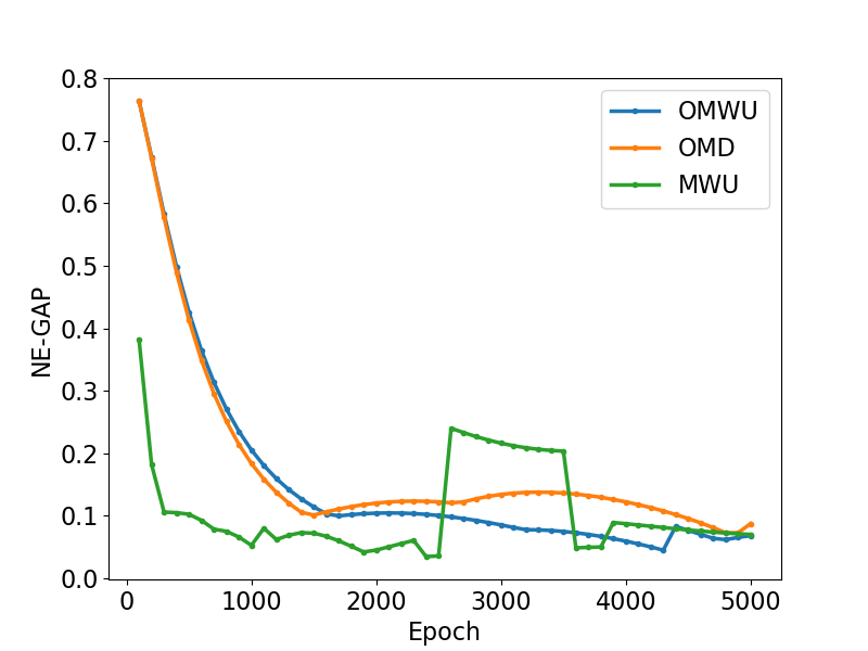
(b) $\log(|V_{\tau}^{\pi^{\star}_{\tau}}-V_{i}|)$ plot

Figure 3: (a) Fictitious play experiment. The red and dark red lines indicate player 0’s value function estimates for states 0 and 1, respectively. The green and dark green lines indicate player 1’s value function estimates for states 0 and 1, respectively. The blue and dark blue lines indicate player 2’s value function estimates for states 0 and 1, respectively. The gray and black lines indicate the sum of each player’s value function estimates for states 0 and 1, respectively. $x$-axis denotes the logarithm with base 2 of the number of iterates (stages) and $y$-axis denotes the value function estimates. (b) Value-iteration-based algorithms with (OMWU, OMD, MWU) NE-ORACLE subroutines. The blue, orange, and green lines indicate $\max_{i\in\mathcal{N}}\max_{s\in{\mathcal{S}}}(V_{i}^{\pi_{i}^{\prime},\pi_{-i}^{(t)}}(s)-V_{i}^{\pi^{(t)}}(s))$ value of the OMWU, OMD, and MWU NE-ORACLE, respectively. $x$-axis denotes the number of iteration of NE-ORACLE subroutine, and $y$-axis denotes the NE-Gap.

7.2 Value-iteration with different NE-ORACLEs

We present an experiment for MZNMGs with different NE-ORACLEs in Section 6. We experimented with an MZNMG $(\mathcal{G}=(\mathcal{N},\mathcal{E}_{Q}),{\mathcal{S}},\mathcal{A},H,(\mathbb{P}_{h})_{h\in[H]},(r_{h,i})_{h\in[H],i\in\mathcal{N}})$ where $\mathcal{N}=[3]$, $\mathcal{E}_{Q}=\{(1,2),(1,3),(2,3)\}$, ${\mathcal{S}}$ = {0,1}, $\mathcal{A}_{i}=\{0,1\}$ for all $i\in\mathcal{N}$, $H=5$, $\mathbb{P}_{h}(s^{\prime}{\,|\,}s,\bm{a}):=\mathbb{F}_{i}(s^{\prime}{\,|\,}s,a_{i})$, $\mathbb{F}_{1}(s^{\prime}{\,|\,}s,a_{1})=\frac{1}{3}\mathbb{P}_{1}(s^{\prime}{\,|\,}s,a_{1})$, $\mathbb{F}_{2}(s^{\prime}{\,|\,}s,a_{2})=\frac{2}{3}\mathbb{P}_{2}(s^{\prime}{\,|\,}s,a_{2})$, $\mathbb{F}_{3}(s^{\prime}{\,|\,}s,a_{3})=0$, $\mathbb{P}_{1}(0{\,|\,}0,1)=\mathbb{P}_{1}(0{\,|\,}1,0)=\mathbb{P}_{2}(0{\,|\,}0,1)=\mathbb{P}_{2}(0{\,|\,}1,0)$ is determined randomly, $\mathbb{P}_{1}(0{\,|\,}1,1)=\mathbb{P}_{1}(0{\,|\,}0,0)=\mathbb{P}_{2}(0{\,|\,}1,1)=\mathbb{P}_{2}(0{\,|\,}0,0)$ is determined randomly, and $r_{h,i}$ is determined randomly that making $(\mathcal{G},\mathcal{A},(r_{h,i}(s))_{i\in\mathcal{N}})$ MZNG for every $h$. We set $\tau=0.05$ for both OMWU and MWU. We set $\eta=1/(36H)$ for both OMWU and OMD. We iterated the algorithm for $T=5000$ times. The result is plotted in Figure 3 (b).

8 Concluding Remarks

We studied a new class of non-cooperative Markov games, i.e., multi-player zero-sum Markov games with networked separable interactions. We established the structural properties of reward and transition dynamics under this model, and showed that marginalizing Markov CCE per state leads to Markov NE. Furthermore, we established the computational hardness of finding Markov stationary CCE in infinite-horizon discounted MZNMGs, unless the underlying network has a star topology, which is in contrast to the tractability of CCE computation for the normal-form special case of MZNMGs, i.e., zero-sum polymatrix games. In light of this hardness result, we focused on 1) star-shaped MZNMGs and developed fictitious-play learning dynamics that provably converges to Markov stationary NE; 2) non-stationary Markov NE computation for general MZNMGs with finite-iteration last-iterate convergence guarantees.

Our work has opened up many venues for future research. Firstly, further study of the fictitious-play property for general MZNMGs beyond star-shaped cases would be interesting, as PPAD-hardness does not necessarily imply the impossibility of asymptotic convergence of FP dynamics in these cases. Additionally, it would be interesting to study model-free online and/or offline RL in MZNMGs, with sample-complexity/regret guarantees, as well as to explore the networked structure beyond the zero-sum setting in non-cooperative Markov games.

Supplementary Materials

In Appendix A, we provide a detailed literature review. In Appendix B, we provide deferred proofs for the results on the MZNMG formulation in Section 3. In Appendix C, we provide deferred proofs for the PPAD-hardness of computing Markov stationary CCE in MZNMGs, in Section 4. In Appendix D, we provide deferred proofs for the fictitious-play property results, in Section 5. In Appendix E, we provide a brief background on stochastic approximation. In Appendix F, we provide deferred proofs for the results regarding Markov non-stationary NE computation in Section 6.

Appendix A Related Work

Tabular Markov game.

Markov games (MG), which are also referred to as stochastic games, were initially introduced by [11] and have since garnered significant attention within the multi-agent RL literature [84, 85]. Early research, such as [12, 86, 87, 88], established asymptotic convergence of various Q-learning-based dynamics in solving MGs. In contrast, recent studies have mainly focused on developing more sample-efficient methods for learning equilibria in two-player zero-sum Markov games, as demonstrated by [89, 90, 91, 37, 92, 63, 93, 23].

Substantial work has also been conducted on learning correlated equilibrium and coarse correlated equilibrium in Markov games, including model-based [92, 94] and model-free approaches [17, 16, 95, 18]. A recently developed algorithm by [22] is able to learn Markov non-stationary CCE while overcoming the curse of multi-agents, whose sample complexity has recently been improved in [39, 38]. Other studies within the full-information feedback setting have focused on proving convergence to CE/CCE and sublinear individual regret [96].

Complexity of equilibrium computation.

Computational challenges can occur for Nash equilibrium-finding in even matrix/normal-form games in general. Computing such equilibria has been proven to be PPAD-complete even for three/two-player general-sum normal-form games [33, 34], which is believed to be computationally hard [50, 97]. Nevertheless, linear programming enables the computation of Nash equilibria in two-player zero-sum games and zero-sum polymatrix games [42]. Alternative solution concepts including (coarse) correlated equilibria are also more favorable than NE when it comes to computational complexity, as they can also be efficiently computed [35, 36]. More recently, [22, 40] have shown that for infinite-horizon discounted Markov games, computing even the coarse correlated equilibrium that is Markov stationary can be PPAD-hard, which is in stark contrast to the stateless normal-form game case. For a recent overview of the computational complexity for equilibrium computation, we refer to [98].

Games with network structure.

Network Games [99] and Graphical Games [100] have been extensively studied in the literature to model the networked interactions among agents. [100] introduced treeNash, an algorithm for computing NE in tree-structured graphical games. The algorithm by [101] can find correlated equilibrium in graphical games. Polymatrix games, wherein edges represent two-player games, constitute a particularly intriguing type of network games. [44] introduced the concept of separable zero-sum games, where a player’s payoff is the sum of their payoffs from pairwise interactions with other players, and provided equilibrium-finding algorithms. [102] demonstrated that graphical games with edges representing zero-sum games (also called pairwise zero-sum polymatrix games) can be reduced to two-person zero-sum games, streamlining the NE computation for this case. [41] established that separable zero-sum multiplayer games can be transformed into pairwise constant-sum polymatrix games. [42] revealed properties of NE in separable zero-sum games, such as non-unique NE payoffs and the reduction of NE computation to CCE computation by marginalizing the equilibria.

More recently, researchers have proposed several NE-finding methods that do not depend on linear programming (LP). [103] employed a continuous-time version of Q-learning to approximate NE in weighted zero-sum polymatrix games, [71] utilized optimistic mirror descent to find NE in constant-sum polymatrix games, and [70] applied optimistic multiplicative weight updates to find NE in zero-sum polymatrix games.

In the setting with state transitions, the networked structure has also been exploited recently in multi-agent RL [104, 105, 106, 107, 108, 109], where either the communication or interaction, in terms of reward or transition, were assumed to have some networked structure. However, most of these results were focused on the cooperative setting (or more generally the potential game setting). We instead focus on a multi-player while non-cooperative, specifically, zero-sum, setting.

Entropy regularization.

Entropy regularization is a common approach used in reinforcement learning to foster exploration and enable faster convergence. Recently, both empirical evidence and provable convergence rate guarantees for entropy-regularized MDPs have been established [110, 111, 112, 113, 114, 115]. In addition to its applications in single-agent RL, entropy regularization has been investigated in game-theoretic settings, including two-player zero-sum matrix games [26], multi-player zero-sum games [103, 70], potential games [80], and extensive-form games [116, 117].

Fictitious play.

Fictitious play is a classical learning dynamics in game theory introduced by [29], in which players develop a belief in their opponent’s policy and use a greedy approach to the belief they hold about the opponent’s policy. (Stochastic) fictitious-play property ((S-)FPP) is a property of a game that ensures the convergence of (stochastic) fictitious play to a Nash equilibrium of the game. In the case of static games, S-FPP holds for two-player zero-sum games [118], 2x$n$ games [119, 120], $n$-player potential games [51], and mean field games [121]. However, FPP normally does not hold for 3x3 games [122]. For stochastic games [11], (S-)FPP holds for zero-sum and identical payoff games [25, 14, 28, 15, 123]. Recently, [123] proved that any stochastic game with turn-based controllers on state transitions has S-FPP, as long as the stage payoffs have S-FPP. For a more detailed overview of fictitious play in stochastic/Markov games, we refer to [124].

Appendix B Omitted Details in Section 3

B.1 Omitted proof for Proposition 1 and Proposition 2

See 1

Proof.

Firstly, in the case with $\mathcal{N}_{C}\neq\emptyset$, we prove that if an MG satisfies the decomposability of the reward function $r_{i}(s,a_{i},\cdot)$ and the transition dynamics $\mathbb{P}(s^{\prime}|s,\cdot)$, then $Q_{i,j}^{V}$ can be decomposed as follows:

$$Q_{i}^{V}(s,\bm{a})=r_{i}(s,\bm{a})+\gamma\mathbb{E}_{s^{\prime}\sim\mathbb{P}(\cdot\mid s,\bm{a})}V(s^{\prime})=\sum_{j\in\mathcal{E}_{Q,i}}r_{i,j}(s,a_{i},a_{j})+\gamma\sum_{j\in\mathcal{N}_{C}}\sum_{s^{\prime}\in{\mathcal{S}}}\mathbb{F}_{j}(s^{\prime}\mid s,a_{j})V(s^{\prime})$$

$$\quad=\sum_{j\in\mathcal{E}_{Q,i}}\left(r_{i,j}(s,a_{i},a_{j})+\gamma\sum_{s^{\prime}\in{\mathcal{S}}}\left(\lambda_{i,j}(s)\boldsymbol{1}(i\in\mathcal{N}_{C})\mathbb{F}_{i}(s^{\prime}\mid s,a_{i})+\boldsymbol{1}(j\in\mathcal{N}_{C})\mathbb{F}_{j}(s^{\prime}\mid s,a_{j})\right)V(s^{\prime})\right)=:\sum_{j\in\mathcal{E}_{Q,i}}Q_{i,j}^{V}(s,a_{i},a_{j}),$$

for any non-negative $(\lambda_{i,j}(s))_{(i,j)\in\mathcal{E}_{Q}}$ such that $\sum_{j\in\mathcal{E}_{Q,i}}\lambda_{i,j}(s)=1$, since by definition $\mathcal{N}_{C}\subseteq\mathcal{E}_{Q,i}$ for every $i\in\mathcal{N}$.

In the case when $\mathcal{N}_{C}=\emptyset$, we prove that if the MG satisfies decomposability of $r_{i}(s,a_{i},\cdot)$ and $\mathbb{P}(\cdot|s,\bm{a})=\mathbb{F}_{o}(\cdot|s)$, then $Q_{i,j}^{V}$ can be decomposed as follows:

$$Q_{i}^{V}(s,\bm{a})=r_{i}(s,\bm{a})+\gamma\mathbb{E}_{s^{\prime}\sim\mathbb{P}(\cdot\mid s,\bm{a})}V(s^{\prime})=\sum_{j\in\mathcal{E}_{Q,i}}\left(r_{i,j}(s,a_{i},a_{j})+\gamma\sum_{s^{\prime}\in{\mathcal{S}}}\lambda_{i,j}(s)\mathbb{F}_{o}(s^{\prime}|s)V(s^{\prime})\right)=:\sum_{j\in\mathcal{E}_{Q,i}}Q_{i,j}^{V}(s,a_{i},a_{j}),$$

for any non-negative $(\lambda_{i,j}(s))_{(i,j)\in\mathcal{E}_{Q}}$ such that $\sum_{j\in\mathcal{E}_{Q,i}}\lambda_{i,j}(s)=1$.

Next, we prove the necessary conditions for an MG to be an MNMG. By definition, we have

$$Q_{i}^{V}(s,\bm{a})=\sum_{j\in\mathcal{E}_{Q,i}}Q_{i,j}^{V}(s,a_{i},a_{j})=r_{i}(s,\bm{a})+\gamma\langle\mathbb{P}(\cdot\mid s,\bm{a}),V(\cdot)\rangle$$

for any $V$, which indicates that

$$\sum_{j\in\mathcal{E}_{Q,i}}(Q_{i,j}^{V}(s,a_{i},a_{j})-Q_{i,j}^{V^{\prime}}(s,a_{i},a_{j}))=\gamma\langle\mathbb{P}(\cdot\mid s,\bm{a}),V(\cdot)-V^{\prime}(\cdot)\rangle,$$

for any $V,V^{\prime}$ and any $(s,\bm{a})$. Since $V$ can be any function, we can do a functional derivative with respect to $V-V^{\prime}$, which means that there exist some functions $\{\mathbb{G}_{i,j}\}_{j\in\mathcal{E}_{Q,i}}$ such that $\mathbb{P}(\cdot\mid s,\bm{a})=\sum_{j\in\mathcal{E}_{Q,i}}\mathbb{G}_{i,j}(\cdot\mid s,a_{i},a_{j})$ for every $i$. Note that the decomposability of $\mathbb{P}$ with respect to $\mathcal{E}_{Q,i}$ above has to hold for all $i\in\mathcal{N}$. Therefore, when $\mathcal{N}_{C}\neq\emptyset$, if $j\notin\mathcal{N}_{C}$, then there exists some $i\in\mathcal{N}$ such that $(i,j)\notin\mathcal{E}_{Q}$. In this case, $\mathbb{P}$ is not dependent on this $j$. So $\mathbb{P}$ should be a function of the players in $\mathcal{N}_{C}$, which indicates that $\mathbb{P}(\cdot\mid s,\bm{a})=\sum_{j\in\mathcal{N}_{C},j\neq i}\mathbb{F}_{i,j}(\cdot\mid s,a_{i},a_{j})$ for every $i$ unless $\mathcal{N}_{C}=\emptyset$. If $\mathcal{N}_{C}=\emptyset$, then it directly concludes that $\mathbb{P}(\cdot\mid s,\bm{a})=\mathbb{F}_{o}(\cdot\mid s)$ for some $\mathbb{F}_{o}$, since by the argument above, it should not depend on any player $j$. Next, we focus on the case when $\mathcal{N}_{C}\neq\emptyset$, and there are more than two players.

Specifically, in this case, if there exist some $k_{1}\neq k_{2}$ and $k_{1}\notin\mathcal{N}_{C}$, such that

$$\mathbb{P}(\cdot|s,\bm{a})=\sum_{i\in\mathcal{N}_{C},i\neq k_{1}}\mathbb{F}_{k_{1},i}(\cdot|s,a_{k_{1}},a_{i})=\sum_{i\in\mathcal{N}_{C},i\neq k_{2}}\mathbb{F}_{k_{2},i}(\cdot|s,a_{k_{2}},a_{i}),$$

then we choose a fixed $a_{k_{1}}$ but changing $a_{k_{2}}$ arbitrarily. This preserves the equality, indicating that

$$\sum_{i\in\mathcal{N}_{C},i\neq k_{1}}\mathbb{F}_{k_{1},i}(\cdot|s,a_{k_{1},\text{fix}},a_{i})=\sum_{i\in\mathcal{N}_{C},i\neq k_{2}}\mathbb{F}_{k_{2},i}(\cdot|s,a_{k_{2}},a_{i})$$ (6)

for any $a_{k_{2}}$. Since $k_{1}\notin\mathcal{N}_{C}$, we can have the left-hand side of (6) written as $\sum_{i\in\mathcal{N}_{C}}\mathbb{F}_{i}(\cdot|s,a_{i})$ by setting $\mathbb{F}_{i}(\cdot|s,a_{i}):=\mathbb{F}_{k_{1},i}(\cdot|s,a_{k_{1},\text{fix}},a_{i})$. Meanwhile, the right-hand side of (6) is also $\mathbb{P}(\cdot|s,\bm{a})$ by definition, which concludes that $\mathbb{P}(\cdot|s,\bm{a})=\sum_{i\in\mathcal{N}_{C}}\mathbb{F}_{i}(\cdot|s,a_{i})$, and proves the theorem. In other words, as long as at least one $k_{1}$ does not belong to $\mathcal{N}_{C}$, we can conclude the theorem.

If no such a $k_{1}\notin\mathcal{N}_{C}$ exists, then it means that all players are in $\mathcal{N}_{C}$. In this case, for any $k_{1}\neq k_{2}$, for a fixed $a_{k_{1},\text{fix}}$, we have

$$\sum_{i\in\mathcal{N}_{C}/\{k_{1}\}}\mathbb{F}_{k_{1},i}(\cdot|s,a_{k_{1},\text{fix}},a_{i})=\sum_{i\in\mathcal{N}_{C}/\{k_{1},k_{2}\}}\mathbb{F}_{k_{2},i}(\cdot|s,a_{k_{2}},a_{i})+\mathbb{F}_{k_{2},k_{1}}(\cdot|s,a_{k_{2}},a_{k_{1},\text{fix}}).$$ (7)

Therefore, if we define $\mathbb{G}_{i}(\cdot|s,a_{i}):=\mathbb{F}_{k_{1},i}(\cdot|s,a_{k_{1},\text{fix}},a_{i})$ for $i\in\mathcal{N}_{C}/\{k_{1},k_{2}\}$, and $\mathbb{G}_{k_{2}}(\cdot|s,a_{k_{2}}):=\mathbb{F}_{k_{1},k_{2}}(\cdot|s,a_{k_{1},\text{fix}},a_{k_{2}})-\mathbb{F}_{k_{2},k_{1}}(\cdot|s,a_{k_{2}},a_{k_{1},\text{fix}})$, then we have

$$\sum_{i\in\mathcal{N}_{C}/\{k_{1},k_{2}\}}\mathbb{F}_{k_{2},i}(\cdot|s,a_{k_{2}},a_{i})=\sum_{i\in\mathcal{N}_{C}/\{k_{1}\}}\mathbb{G}_{i}(\cdot|s,a_{i}).$$ (8)

Let $k_{3}\in\mathcal{N}_{C}$ such that $k_{3}\neq k_{1},k_{2}$. By definition of $\mathbb{F}_{i,j}$, we have

$$\mathbb{P}(\cdot|s,\bm{a}) =\sum_{i\in\mathcal{N}_{C}/\{k_{3}\}}\mathbb{F}_{k_{3},i}(\cdot|s,a_{k_{3}},a_{i})=\sum_{i\in\mathcal{N}_{C}/\{k_{2}\}}\mathbb{F}_{k_{2},i}(\cdot|s,a_{k_{2}},a_{i}).$$

Plugging (8), we have

$$\mathbb{P}(\cdot|s,\bm{a}) =\sum_{i\in\mathcal{N}_{C}/\{k_{3}\}}\mathbb{F}_{k_{3},i}(\cdot|s,a_{k_{3}},a_{i})=\sum_{i\in\mathcal{N}_{C}/\{k_{1}\}}\mathbb{G}_{i}(\cdot|s,a_{i})+\mathbb{F}_{k_{2},k_{1}}(\cdot|s,a_{k_{2}},a_{k_{1}})$$ (9)

for any $\bm{a}\in\mathcal{A}$. If we now fix $a_{k_{3}}$ as $a_{k_{3},\text{fix}}$, then from (9) we know that

$$\sum_{i\in\mathcal{N}_{C}/\{k_{3}\}}\mathbb{F}_{k_{3},i}(\cdot|s,a_{k_{3},\text{fix}},a_{i})=\sum_{i\in\mathcal{N}_{C}/\{k_{1},k_{3}\}}\mathbb{G}_{i}(\cdot|s,a_{i})+\mathbb{G}_{k_{3}}(\cdot|s,a_{k_{3},\text{fix}})+\mathbb{F}_{k_{2},k_{1}}(\cdot|s,a_{k_{2}},a_{k_{1}}).$$ (10)

Plugging (10) to (9), we have

$$\mathbb{P}(\cdot|s,\bm{a}) =\sum_{i\in\mathcal{N}_{C}/\{k_{1},k_{3}\}}\mathbb{G}_{i}(\cdot|s,a_{i})+\mathbb{F}_{k_{2},k_{1}}(\cdot|s,a_{k_{2}},a_{k_{1}})+\mathbb{G}_{k_{3}}(\cdot|s,a_{k_{3}})$$

$$=\sum_{i\in\mathcal{N}_{C}/\{k_{3}\}}\mathbb{F}_{k_{3},i}(\cdot|s,a_{k_{3},\text{fix}},a_{i})-\mathbb{G}_{k_{3}}(\cdot|s,a_{k_{3},\text{fix}})+\mathbb{G}_{k_{3}}(\cdot|s,a_{k_{3}})=:\sum_{i\in\mathcal{N}_{C}}\mathbb{F}_{i}(\cdot|s,a_{i})$$

where $\mathbb{F}_{i}(\cdot|s,a_{i}):=\mathbb{F}_{k_{3},i}(\cdot|s,a_{k_{3},\text{fix}},a_{i})$ for $i\in\mathcal{N}_{C}/\{k_{3}\}$ and $\mathbb{F}_{k_{3}}(\cdot|s,a_{k_{3}}):=-\mathbb{G}_{k_{3}}(\cdot|s,a_{k_{3},\text{fix}})+\mathbb{G}_{k_{3}}(\cdot|s,a_{k_{3}})$, which concludes the decomposability of the transition dynamics. Finally, note that we can ensure the non-negativity of $\mathbb{F}_{i}$, since we can iterate the following procedure:

Algorithm 3 Procedure for Constructing Non-Negative $\{\mathbb{F}_{i}\}_{i\in\mathcal{N}_{C}}$

  while there exists $s,s^{\prime}\in{\mathcal{S}}$ and $i\in\mathcal{N}_{C}$ such that $\min_{a_{i}\in\mathcal{A}_{i}}\mathbb{F}_{i}(s^{\prime}|s,a_{i})<0$ do

     Set $s,s^{\prime}\in{\mathcal{S}}$ and $i\in\mathcal{N}_{C}$ that satisfying $\min_{a_{i}\in\mathcal{A}_{i}}\mathbb{F}_{i}(s^{\prime}|s,a_{i})<0$

     Sort $\mathcal{N}_{C}$ according to the descending order of $b_{k}:=\min_{a_{k}\in\mathcal{A}_{k}}\mathbb{F}_{k}(s^{\prime}|s,a_{k})$, and denote it as $\{j_{1},j_{2},\dots,j_{|\mathcal{N}_{C}|}\}$

     Define $\text{tmp1}=0,t=1$

     while $\text{tmp1}<-\min_{a_{i}\in\mathcal{A}_{i}}\mathbb{F}_{i}(s^{\prime}|s,a_{i})$ do

        Define $\text{tmp2}=-\min_{a_{i}\in\mathcal{A}_{i}}\mathbb{F}_{i}(s^{\prime}|s,a_{i})-\text{tmp1}>0$

        Define $\text{tmp3}=\min(\min_{a_{j_{t}}\in\mathcal{A}_{j_{t}}}\mathbb{F}_{j_{t}}(s^{\prime}|s,a_{j_{t}}),\text{tmp2})>0$;

        Update $\mathbb{F}_{j_{t}}(s^{\prime}|s,a_{j_{t}})\leftarrow\mathbb{F}_{j_{t}}(s^{\prime}|s,a_{j_{t}})-\text{tmp3}$ for all $a_{j_{t}}\in\mathcal{A}_{j_{t}}$

        Update $\mathbb{F}_{i}(s^{\prime}|s,a_{i})\leftarrow\mathbb{F}_{i}(s^{\prime}|s,a_{i})+\text{tmp3}$ for all $a_{i}\in\mathcal{A}_{i}$

        Update $\text{tmp1}\leftarrow\text{tmp1}+\text{tmp3}$ and $t\leftarrow t+1$

     end while

  end while

In this context, the third and fourth lines of the inner-while loop ensure that $\mathbb{P}(s^{\prime}|s,\bm{a})=\sum_{j\in\mathcal{N}_{C}}\mathbb{F}_{j}(s^{\prime}|s,a_{j})$ always holds for $s,s^{\prime}\in{\mathcal{S}}$, $\bm{a}\in\mathcal{A}$. Furthermore, $\text{tmp}3$ remains greater than 0 within the inner-while loop. This is because if $\min_{a_{j_{t}}\in\mathcal{A}_{j_{t}}}\mathbb{F}_{j_{t}}(s^{\prime}|s,a_{j_{t}})\leq 0$, then it implies that $\min_{a_{j_{k}}\in\mathcal{A}_{j_{k}}}\mathbb{F}_{j_{k}}(s^{\prime}|s,a_{j_{k}})=0$ for all $k\in[t]$. Also, $\min_{a_{j_{k}}\in\mathcal{A}_{j_{k}}}\mathbb{F}_{j_{k}}(s^{\prime}|s,a_{j_{k}})\leq\min_{a_{j_{t}}\in\mathcal{A}_{j_{t}}}\mathbb{F}_{j_{t}}(s^{\prime}|s,a_{j_{t}})\leq 0$ for every $k\in[|\mathcal{N}_{C}|]$. Meanwhile, since we assumed $\min_{a_{i}\in\mathcal{A}_{i}}\mathbb{F}_{i}(s^{\prime}|s,a_{i})<0$, we can define a vector $\widetilde{a}$ with elements $\widetilde{a}_{j}\in\mathop{\mathrm{argmin}}_{a_{j}\in\mathcal{A}_{j}}\mathbb{F}_{j}(s^{\prime}|s,a_{j})$. This implies that $\mathbb{P}(s^{\prime}|s,\widetilde{a})=\sum_{i\in\mathcal{N}_{C}}\min_{a_{i}\in\mathcal{A}_{i}}\mathbb{F}_{i}(s^{\prime}|s,a_{i})<0$, which contradicts the condition $\mathbb{P}(s^{\prime}|s,\widetilde{a})\geq 0$.

Therefore, our procedure ensures that the number of pairs $(s,s^{\prime})\in{\mathcal{S}}\times{\mathcal{S}}$ and indexes $i\in\mathcal{N}_{C}$ for which $\min_{a_{i}\in\mathcal{A}_{i}}\mathbb{F}_{i}(s^{\prime}|s,a_{i})<0$ is consistently reduced.

If there are only two players, then both of them belong to $\mathcal{N}_{C}$. However, one cannot decompose the transition dynamics as above, as there is no such a $k_{3}\neq k_{1},k_{2}$ to construct the aforementioned formula. Indeed, any two-player (zero-sum) MG satisfies our definition of M(Z)NMGs in Definition 1.

For the reward decomposition, if $\mathcal{N}_{C}\neq\emptyset$, we have

$$r_{i}(s,\bm{a})=\sum_{j\in\mathcal{E}_{Q,i}}\left(Q_{i,j}^{V}(s,a_{i},a_{j})-\gamma\langle\boldsymbol{1}(j\in\mathcal{N}_{C})\mathbb{F}_{j}(\cdot\mid s,a_{j}),V(\cdot)\rangle\right)$$

and if $\mathcal{N}_{C}=\emptyset$, we have

$$r_{i}(s,\bm{a})=\sum_{j\in\mathcal{E}_{Q,i}}\left(Q_{i,j}^{V}(s,a_{i},a_{j})-\gamma\langle\frac{1}{|\mathcal{E}_{Q,i}|}\mathbb{F}_{o}(\cdot\mid s),V(\cdot)\rangle\right).$$

Hence, $r_{i}(s,a_{i},\cdot)$ can be represented as $r_{i}(s,\bm{a})=\sum_{j\in\mathcal{E}_{Q,i}}r_{i,j}(s,a_{i},a_{j})$ for some functions $(r_{i,j})_{(i,j)\in\mathcal{E}_{Q}}$. The same procedure as Algorithm 3 provides that we can ensure the non-negativity of $r_{i,j}$, so that $r_{i}(s,a_{i},\cdot)$ is decomposable with respect to $\mathcal{E}_{Q,i}$. In fact, adding any large-enough constant to $r_{i,j}$ does not change the solution to the problem, while ensuring the non-negativity of $r_{i,j}$. ∎

Proposition 1 - Finite-horizon version. For a given graph $\mathcal{G}=(\mathcal{N},\mathcal{E}_{Q})$, an MG $(\mathcal{N},{\mathcal{S}},\mathcal{A},(\mathbb{P}_{h})_{h\in[H]},(r_{h,i})_{i\in\mathcal{N},h\in[H]})$ with more than two players is an MNMG with $\mathcal{G}$ if and only if: (1) $r_{h,i}(s,a_{i},\cdot)$ is decomposable with respect to $\mathcal{E}_{Q,i}$ for each $i\in\mathcal{N}\,,s\in{\mathcal{S}}\,,a_{i}\in\mathcal{A}_{i},\,h\in[H]$, i.e., $r_{h,i}(s,\bm{a})=\sum_{j\in\mathcal{E}_{Q,i}}r_{h,i,j}(s,a_{i},a_{j})$ for a set of functions $\{r_{h,i,j}(s,a_{i},\cdot)\}_{j\in\mathcal{E}_{Q,i}}$ and (2) the transition dynamics $\mathbb{P}_{h}(s^{\prime}|s,\cdot)$ is decomposable with respect to$\mathcal{N}_{C}$ corresponding to this $\mathcal{G}$ for all $h\in[H]$, i.e., $\mathbb{P}_{h}(s^{\prime}|s,\bm{a})=\sum_{i\in\mathcal{N}_{C}}\mathbb{F}_{h,i}(s^{\prime}|s,a_{i})$ for a set of functions $\{\mathbb{F}_{h,i}(s^{\prime}|s,\cdot)\}_{i\in\mathcal{N}_{C}}$ if $\mathcal{N}_{C}\neq\emptyset$, or $\mathbb{P}_{h}(s^{\prime}|s,\bm{a})=\mathbb{F}_{h,o}(s^{\prime}|s)$ for some constant function (of $\bm{a}$) $\mathbb{F}_{h,o}(s^{\prime}|s)$ if $\mathcal{N}_{C}=\emptyset$. Moreover, an MG qualifies as an MZNMG if and only if it satisfies an additional condition: the MNG, characterized by $(\mathcal{G},\mathcal{A},(r_{h,i,j}(s))_{(i,j)\in\mathcal{E}_{Q}})$, must be an MZNG for all $s\in{\mathcal{S}},h\in[H]$. In the case with two players, every (zero-sum) Markov game becomes an M(Z)NMG.

Proposition 2 (Decomposition of $(Q_{i}^{V})_{i\in\mathcal{N}}$). For an infinite-horizon $\gamma$-discounted MNMG with $\mathcal{G}=(\mathcal{N},\mathcal{E}_{Q})$ such that $\mathcal{N}_{C}\neq\emptyset$, if we know that $\mathbb{P}(s^{\prime}|s,\bm{a})=\sum_{i\in\mathcal{N}_{C}}\mathbb{F}_{i}(s^{\prime}|s,a_{i})$, and $r_{i}(s,\bm{a})=\sum_{j\in\mathcal{E}_{Q,i}}r_{i,j}(s,a_{i},a_{j})$ for some $\{\mathbb{F}_{i}\}_{i\in\mathcal{N}_{C}}$ and $\{r_{i,j}\}_{(i,j)\in\mathcal{E}_{Q}}$, then the $Q_{i,j}^{V}$ given in Definition 1 can be represented as

$$Q_{i,j}^{V}(s,a_{i},a_{j})=r_{i,j}(s,a_{i},a_{j})+\sum_{s^{\prime}\in{\mathcal{S}}}\gamma\left(\boldsymbol{1}(j\in\mathcal{N}_{C})\mathbb{F}_{j}(s^{\prime}\mid s,a_{j})+\boldsymbol{1}(i\in\mathcal{N}_{C})\lambda_{i,j}(s)\mathbb{F}_{i}(s^{\prime}\mid s,a_{i})\right)V(s^{\prime})$$

for any non-negative $(\lambda_{i,j}(s))_{(i,j)\in\mathcal{E}_{Q}}$ such that $\sum_{j\in\mathcal{E}_{Q,i}}\lambda_{i,j}(s)=1$ for all $i\in\mathcal{N}$ and $s\in{\mathcal{S}}$. For an infinite-horizon $\gamma$-discounted MNMG with $\mathcal{G}=(\mathcal{N},\mathcal{E}_{Q})$ such that $\mathcal{N}_{C}=\emptyset$, if we know that $\mathbb{P}(s^{\prime}|s,\bm{a})=\mathbb{F}_{o}(s^{\prime}|s)$, and $r_{i}(s,\bm{a})=\sum_{j\in\mathcal{E}_{Q,i}}r_{i,j}(s,a_{i},a_{j})$ for some $\mathbb{F}_{o}$ and $\{r_{i,j}\}_{(i,j)\in\mathcal{E}_{Q}}$, then the $Q_{i,j}^{V}$ given in Definition 1 can be represented as

$$Q_{i,j}^{V}(s,a_{i},a_{j})=r_{i,j}(s,a_{i},a_{j})+\sum_{s^{\prime}\in{\mathcal{S}}}\gamma\left(\lambda_{i,j}(s)\mathbb{F}_{o}(s^{\prime}\mid s)\right)V(s^{\prime})$$

for any non-negative $(\lambda_{i,j}(s))_{(i,j)\in\mathcal{E}_{Q}}$ such that $\sum_{j\in\mathcal{E}_{Q,i}}\lambda_{i,j}(s)=1$ for all $i\in\mathcal{N}$ and $s\in{\mathcal{S}}$. We call it the canonical decomposition of $\{Q_{i}^{V}\}_{i\in\mathcal{N}}$ when $Q_{i,j}^{V}$ can be represented as above with $\lambda_{i,j}(s)={1}/{|\mathcal{E}_{Q,i}|}$ for $j\in\mathcal{E}_{Q,i}$.

Proposition 2 naturally follows from the proof of Proposition 1 (a).

Proposition 2 - Finite-horizon version (Decomposition of $(Q_{h,i}^{V})_{i\in\mathcal{N}}$). For a finite-horizon MNMG with $\mathcal{G}=(\mathcal{N},\mathcal{E}_{Q})$ with $\mathcal{N}_{C}\neq\emptyset$, we know $\mathbb{P}_{h}(s^{\prime}|s,\bm{a})=\sum_{i\in\mathcal{N}_{C}}\mathbb{F}_{h,i}(s^{\prime}|s,a_{i})$, and $r_{h,i}(s,\bm{a})=\sum_{j\in\mathcal{E}_{Q,i}}r_{h,i,j}(s,a_{i},a_{j})$ for some $\{\mathbb{F}_{h,i}\}_{i\in\mathcal{N}_{C}}$ and $\{r_{h,i,j}\}_{(i,j)\in\mathcal{E}_{Q}}$, then the $Q_{h,i,j}^{V}$ given in Definition 1 can be represented as

$$Q_{h,i,j}^{V}(s,a_{i},a_{j})=r_{h,i,j}(s,a_{i},a_{j})+\sum_{s^{\prime}\in{\mathcal{S}}}\left(\boldsymbol{1}(j\in\mathcal{N}_{C})\mathbb{F}_{h,j}(s^{\prime}\mid s,a_{j})+\boldsymbol{1}(i\in\mathcal{N}_{C})\lambda_{h,i,j}(s)\mathbb{F}_{h,i}(s^{\prime}\mid s,a_{i})\right)V_{h+1}(s^{\prime})$$

for any non-negative $(\lambda_{h,i,j}(s))_{(i,j)\in\mathcal{E}_{Q}}$ such that $\sum_{j\in\mathcal{E}_{Q,i}}\lambda_{h,i,j}(s)=1$ for all $i\in\mathcal{N}$, $s\in{\mathcal{S}}$, and $h\in[H]$. For a finite-horizon MNMG with $\mathcal{G}=(\mathcal{N},\mathcal{E}_{Q})$ such that $\mathcal{N}_{C}=\emptyset$, $\mathbb{P}_{h}(s^{\prime}|s,\bm{a})=\mathbb{F}_{h,o}(s^{\prime}|s)$, and $r_{h,i}(s,\bm{a})=\sum_{j\in\mathcal{E}_{Q,i}}r_{h,i,j}(s,a_{i},a_{j})$ for some $\mathbb{F}_{h,o}$ and $\{r_{h,i,j}\}_{(i,j)\in\mathcal{E}_{Q}}$, the $Q_{h,i,j}^{V}$ given in Definition 1 can be represented as

$$Q_{h,i,j}^{V}(s,a_{i},a_{j})=r_{h,i,j}(s,a_{i},a_{j})+\sum_{s^{\prime}\in{\mathcal{S}}}\left(\lambda_{h,i,j}(s)\mathbb{F}_{h,o}(s^{\prime}\mid s)\right)V_{h+1}(s^{\prime})$$

for any non-negative $(\lambda_{h,i,j}(s))_{(i,j)\in\mathcal{E}_{Q}}$ such that $\sum_{j\in\mathcal{E}_{Q,i}}\lambda_{h,i,j}(s)=1$ for all $i\in\mathcal{N}$, $s\in{\mathcal{S}}$, and $h\in[H]$. We call it the canonical decomposition of $Q$-value functions when $Q_{h,i,j}^{V}$ can be represented as above with $\lambda_{h,i,j}(s)={1}/{|\mathcal{E}_{Q,i}|}$ for $j\in\mathcal{E}_{Q,i}$.

B.2 An alternative definition of MNMGs

Definition 3 (An alternative definition of MNMGs).

An infinite-horizon $\gamma$-discounted MG is called a Multi-player MG with Networked separable interactions (MNMG) characterized by a tuple

$$(\mathcal{G}=(\mathcal{N},\mathcal{E}_{Q}),{\mathcal{S}},\mathcal{A},\mathbb{P},(r_{i})_{i\in\mathcal{N}},\gamma)$$

if for any policy $\pi$, there exist a set of functions $(Q_{i,j}^{\pi})_{(i,j)\in\mathcal{E}_{Q}}$ and an undirected connected graph $\mathcal{G}=(\mathcal{N},\mathcal{E}_{Q})$ such that $Q_{i}^{\pi}(s,\bm{a})=\sum_{j\in\mathcal{E}_{Q,i}}Q_{i,j}^{\pi}(s,a_{i},a_{j})$ holds for every $i\in\mathcal{N}$, $s\in{\mathcal{S}}$, $\bm{a}\in\mathcal{A}$. A finite-horizon MG is called a Multi-player MG with Networked separable interactions if for any policy $\pi$, there exist a set of functions $(Q_{h,i,j}^{\pi})_{(i,j)\in\mathcal{E}_{Q},h\in[H]}$ such that $Q_{h,i}^{\pi}(s,\bm{a})=\sum_{j\in\mathcal{E}_{Q,i}}Q_{h,i,j}^{\pi}(s,a_{i},a_{j})$ holds for every $i\in\mathcal{N}$, $s\in{\mathcal{S}}$, $\bm{a}\in\mathcal{A}$, and $h\in[H]$.

The “if” condition of Proposition 1 also holds for this definition. However, the proof for the “only if” condition of Proposition 1 uses the functional derivative argument. We cannot use the functional derivative here directly, since $\bm{V}^{\pi}:=(V^{\pi}(s))_{s\in{\mathcal{S}}}$ cannot represent all vectors in $[0,R/(1-\gamma)]^{|{\mathcal{S}}|}$. To be specific, we have

$$Q_{i}^{\pi}(s,\bm{a})=\sum_{j\in\mathcal{E}_{Q,i}}Q_{i,j}^{\pi}(s,a_{i},a_{j})=r_{i}(s,\bm{a})+\gamma\langle\mathbb{P}(\cdot\mid s,\bm{a}),V_{i}^{\pi}(\cdot)\rangle$$

for any policies $\pi,\pi^{\prime}$, which indicates

$$\sum_{j\in\mathcal{E}_{Q,i}}(Q_{i,j}^{\pi}(s,a_{i},a_{j})-Q_{i,j}^{\pi^{\prime}}(s,a_{i},a_{j}))=\gamma\langle\mathbb{P}(\cdot\mid s,\bm{a}),V_{i}^{\pi}(\cdot)-V_{i}^{\pi^{\prime}}(\cdot)\rangle.$$ (11)

If we can find a set of policies $(\pi^{(k)})_{k\in[|{\mathcal{S}}|]}$ such that the vectors in $\{\bm{V}_{i}^{\pi^{(k)}}-\bm{V}_{i}^{\pi^{\prime}}\}_{k\in[|{\mathcal{S}}|]}$ are independent for some fixed $\pi^{\prime}$, then we can concatenate the vectors $\{\bm{V}_{i}^{\pi^{(k)}}-\bm{V}_{i}^{\pi^{\prime}}\}_{k\in[|{\mathcal{S}}|]}$ together as a matrix of size $|{\mathcal{S}}|\times|{\mathcal{S}}|$ that is full-rank, and solve for $\mathbb{P}(\cdot{\,|\,}s,\bm{a})$ by solving the linear equations (11), for some fixed $(s,\bm{a})$. This way, we can show that $\mathbb{P}(\cdot{\,|\,}s,\bm{a})=\sum_{j\in\mathcal{E}_{Q,i}}\mathbb{F}_{i,j}(\cdot{\,|\,}s,a_{i},a_{j})$, and the rest of the proof follows from that of Proposition 1. However, such a set of policies $(\pi^{(k)})_{k\in[|{\mathcal{S}}|]}$ (and $\pi^{\prime}$) may not exist in some degenerate cases, as to be detailed below.

Definition 4 (Degenerate MG with respect to player $i$).

We call an MG degenerate with respect to player $i\in\mathcal{N}$ if there exists some $s\in{\mathcal{S}}$ such that for any $\pi$, $Q^{\pi}_{i}(s,\bm{a})$ is a constant function of $\bm{a}\in\mathcal{A}$.

Definition 5 (Non-degenerate MG).

We call an MG non-degenerate if an MG is not degenerate with respect to any player $i\in\mathcal{N}$.

Now, we are ready to state the counterpart of Proposition 1 in these non-degenerate cases. The proof for the “if” direction is exactly the same as that of Proposition 1. We focus on the proof of the “only if” statement.

Proposition 1 - An alternative definition version. For a given graph $\mathcal{G}=(\mathcal{N},\mathcal{E}_{Q})$, a non-degenerate MG $(\mathcal{N},{\mathcal{S}},\mathcal{A},\mathbb{P},(r_{i})_{i\in\mathcal{N}},\gamma)$ (in the sense of Definition 5) with more than two players is an MNMG with $\mathcal{G}$ if and only if: (1) $r_{i}(s,a_{i},\cdot)$ is decomposable with respect to $\mathcal{E}_{Q,i}$ for each $i\in\mathcal{N},s\in{\mathcal{S}},a_{i}\in\mathcal{A}_{i}$, i.e., $r_{i}(s,\bm{a})=\sum_{j\in\mathcal{E}_{Q,i}}r_{i,j}(s,a_{i},a_{j})$ for a set of functions $\{r_{i,j}(s,a_{i},\cdot)\}_{j\in\mathcal{E}_{Q,i}}$, and (2) the transition dynamics $\mathbb{P}(s^{\prime}|s,\cdot)$ is decomposable with respect to the $\mathcal{N}_{C}$ corresponding to this $\mathcal{G}$, i.e., $\mathbb{P}(s^{\prime}|s,\bm{a})=\sum_{i\in\mathcal{N}_{C}}\mathbb{F}_{i}(s^{\prime}|s,a_{i})$ for a set of functions $\{\mathbb{F}_{i}(s^{\prime}|s,\cdot)\}_{i\in\mathcal{N}_{C}}$ if $\mathcal{N}_{C}\neq\emptyset$, or $\mathbb{P}(s^{\prime}|s,\bm{a})=\mathbb{F}_{o}(s^{\prime}|s)$ for some constant function (of $\bm{a}$) $\mathbb{F}_{o}(s^{\prime}|s)$ if $\mathcal{N}_{C}=\emptyset$.

Proof.

Proofs of the claims are deferred to Section B.3 to preserve the flow of the argument.

Claim 1.

For player $i\in\mathcal{N}$, if there exists a policy $\pi$ such that for every $s\in{\mathcal{S}}$, there exist $\bm{a}_{s,1},\bm{a}_{s,2}$ that make $Q_{i}^{\pi}(s,\bm{a}_{s,1})\neq Q_{i}^{\pi}(s,\bm{a}_{s,2})$, then we can construct $|{\mathcal{S}}|$ number of policies $(\pi^{(k)})_{k\in[|{\mathcal{S}}|]}$ such that $\{\bm{V}_{i}^{\pi^{(k)}}-\bm{V}_{i}^{\pi}\}_{k\in[|{\mathcal{S}}|]}$ are independent for any fixed $\pi$.

Therefore, for player $i\in\mathcal{N}$, if the condition of 1 holds, then we can guarantee that there exist some functions $\{\mathbb{G}_{i,j}\}_{j\in\mathcal{E}_{Q,i}}$ such that $\mathbb{P}(\cdot|s,\bm{a})=\sum_{j\in\mathcal{E}_{Q,i}}\mathbb{G}_{i,j}(\cdot|s,a_{i},a_{j})$, by the argument after Equation 11. If we assume that the condition of 1 holds for every player $i\in\mathcal{N}$, then there exist some functions $\{\mathbb{G}_{i,j}\}_{(i,j)\in\mathcal{E}_{Q}}$ such that $\mathbb{P}(\cdot|s,\bm{a})=\sum_{j\in\mathcal{E}_{Q,i}}\mathbb{G}_{i,j}(\cdot|s,a_{i},a_{j})$ for every $i\in\mathcal{N}$. Then, we can prove the decomposability of $\mathbb{P}(s^{\prime}|s,\cdot)$ with respect to $\mathcal{N}_{C}$ with the same steps as Equations (6) - (10).

Hence, by 1, we only need to prove that if an MG is non-degenerate with respect to player $i$, then there exists a policy $\pi$ such that there exist $\bm{a}_{s,1},\bm{a}_{s,2}$ that make $Q_{i}^{\pi}(s,\bm{a}_{s,1})\neq Q_{i}^{\pi}(s,\bm{a}_{s,2})$ for every $s\in{\mathcal{S}}$. If $|\mathcal{A}|=1$, then the transition dynamics are already decomposed, so we do not need to consider this case.

Claim 2.

Assume $|\mathcal{A}|\geq 2$. For player $i\in\mathcal{N}$, assume that for any policy $\pi$, there exists a state $s_{\pi}\in{\mathcal{S}}$ such that $Q^{\pi}_{i}(s_{\pi},\bm{a})$ is a constant function of $\bm{a}$. Then, there exists a state $s\in{\mathcal{S}}$ such that uniformly for any policy $\pi$, $Q^{\pi}_{i}(s,\bm{a})$ is a constant function of $\bm{a}$.

2 shows that if the assumption of 1 does not hold for player $i\in\mathcal{N}$, then

$${\mathcal{S}}_{\text{const},i}:=\{s\mid\text{For any }\pi,Q^{\pi}_{i}(s,\bm{a})\text{ is a constant function of }\bm{a}\}$$

is not an empty set. By Definition 4, if an MG is not degenerate with respect to player $i$, then ${\mathcal{S}}_{\text{const},i}$ is empty, and thus the conditions of 1 always hold for player $i$. Therefore, if we assume the non-degeneracy of MG (Definition 5), by 1 and the arguments immediately following it, $\mathbb{P}(s^{\prime}|s,\cdot)$ is decomposable with respect to $\mathcal{N}_{C}$. ∎

Remark 6 (Degenerate MG with respect to player $i$).

The degeneracy of MGs as defined above can indeed be rare. To illustrate, consider a seemingly degenerate scenario where for all $s\in{\mathcal{S}}$, $r_{i}(s,\bm{a})$ remains a constant function with respect to $\bm{a}$; even under such circumstances, it is possible for the MG to be non-degenerate with respect to player $i$. For example, assume that $\mathcal{N}=[2],\gamma=\frac{1}{2}$, ${\mathcal{S}}=\{-1,1\}$ $\mathcal{A}_{i}=\{-1,1\}$, $\mathbb{P}(s^{\prime}{\,|\,}s,a_{1},a_{2})=\boldsymbol{1}(s^{\prime}=sa_{1}a_{2}),r_{1}(s,\bm{a})=r_{2}(s,\bm{a})=(1+s)$. Let $\pi$ satisfy $\pi(\bm{a}{\,|\,}1)=\boldsymbol{1}(a_{1}=1,a_{2}=-1),\pi(\bm{a}{\,|\,}-1)=\boldsymbol{1}(a_{1}=-1,a_{2}=-1)$. Then, we have $V^{\pi}_{1}(1)=2+\frac{1}{2}V^{\pi}_{1}(-1)$ and $V^{\pi}_{1}(-1)=\frac{1}{2}V^{\pi}_{1}(-1)$, which further means $V^{\pi}_{1}(-1)=0$ and $V^{\pi}_{1}(1)=2$, i.e., $V^{\pi}_{1}(s)=1+s$ always holds. As a result, $Q^{\pi}_{1}(1,\bm{a})=1+s+\frac{1}{2}\left(sa_{1}a_{2}+1\right)$, which is not a constant function, and the game is thus non-degenerate with respect to agent $i$. Moreover, suppose that the policy, transition dynamics, and reward functions are randomly chosen. The measure of the event that the existence of $s\in{\mathcal{S}}$ such that $Q_{i}^{\pi}(s,\bm{a})$ is constant for all possible actions $\bm{a}$ under this randomly chosen policy, transition dynamics, and reward function is 0. This is primarily because $Q_{i}^{\pi}(s,\cdot):\mathcal{A}\to\mathbb{R}$ must lie on a particular hyperplane in the overall value function space, which takes measure $0$. Oftentimes, different actions will transition to different states and yield different rewards, thereby generating almost unique $Q_{i}^{\pi}(s,\bm{a})$ values.

Remark 7.

If we have more than two players that satisfy the condition of 1, i.e., the MG is non-degenerate with respect to more than two players (instead of being non-degenerate with respect to all players), then we can still guarantee the decomposability of $\mathbb{P}(s^{\prime}{\,|\,}s,\cdot)$ with respect to a set that is not necessarily the same as $\mathcal{N}_{C}$. As a byproduct of the decomposability of $\mathbb{P}(s^{\prime}{\,|\,}s,\cdot)$, we can guarantee the decomposability of $r_{i}(s,a_{i},\cdot)$, too.

B.3 Deferred proof of the claims in Section B.2

We define $\Pi:=\begin{bmatrix}\pi(s_{1})&0&\cdots&0\\ 0&\pi(s_{2})&\cdots&0\\ \vdots&\vdots&\ddots&0\\ 0&0&\cdots&\pi(s_{|{\mathcal{S}}|})\end{bmatrix}\in\mathbb{R}^{|{\mathcal{S}}||\mathcal{A}|\times|{\mathcal{S}}|}$, where $\pi(s)$ is a column vector for the policy at state $s$, $\bm{P}:=(\mathbb{P}(s^{\prime}{\,|\,}s,\bm{a}))_{((s,\bm{a}),s^{\prime})}$, $\bm{R}:=\begin{bmatrix}\bm{r}(s_{1})^{\intercal}&0&\cdots&0\\ 0&\bm{r}(s_{2})^{\intercal}&\cdots&0\\ \vdots&\vdots&\ddots&0\\ 0&0&\cdots&\bm{r}(s_{|{\mathcal{S}}|})^{\intercal}\end{bmatrix}\in\mathbb{R}^{|{\mathcal{S}}|\times|{\mathcal{S}}||\mathcal{A}|}$, then we have $\bm{V}_{i}^{\pi}=(I-\gamma\Pi^{\intercal}\bm{P})^{-1}\bm{R}\Pi\boldsymbol{1}\in\mathbb{R}^{|{\mathcal{S}}|}$ where $\boldsymbol{1}\in\mathbb{R}^{|{\mathcal{S}}|}$ is $(1,\dots,1)^{\intercal}$.

Proof of 1.

If we differentiate $\bm{V}_{i}^{\pi}$ with respect to $\pi$ along the direction $\Delta_{(s,\bm{a}_{1},\bm{a}_{2})}:=\bm{e}_{\bm{a}_{1},s}-\bm{e}_{\bm{a}_{2},s}{\in\mathbb{R}^{|\mathcal{A}||{\mathcal{S}}|}}$ for some $\bm{a}_{1},\bm{a}_{2}\in\mathcal{A}$, i.e., the direction that increases (or decreases) $\pi(\bm{a}_{1}{\,|\,}s)$ and decreases (or increases) $\pi(\bm{a}_{2}{\,|\,}s)$, respectively, then by computation, we can have the following directional derivative:

$$\nabla_{\Delta_{(s,\bm{a}_{1},\bm{a}_{2})}}\bm{V}_{i}^{\pi} =(I-\gamma\Pi^{\intercal}\bm{P})^{-1}\left(\sum_{s^{\prime}\in{\mathcal{S}}}\left(\mathbb{P}(s^{\prime}|s,\bm{a}_{1})V_{i}^{\pi}(s^{\prime})-\mathbb{P}(s^{\prime}{\,|\,}s,\bm{a}_{2})V_{i}^{\pi}(s^{\prime})\right)+r_{i}(s,\bm{a}_{1})-r_{i}(s,\bm{a}_{2})\right)\bm{e}_{s}$$

$$=\left(Q_{i}^{\pi}(s,\bm{a}_{1})-Q_{i}^{\pi}(s,\bm{a}_{2})\right)(I-\gamma\Pi^{\intercal}\bm{P})^{-1}\bm{e}_{s}.$$ (12)

Therefore, if there exists a policy $\pi$ such that for every $s$, there exist $\bm{a}_{s,1},\bm{a}_{s,2}$ that make $Q_{i}^{\pi}(s,\bm{a}_{s,1})\neq Q_{i}^{\pi}(s,\bm{a}_{s,2})$, then deviating from $\pi$ along the $\Delta_{(s,\bm{a}_{s,1},\bm{a}_{s,2})}$ direction for every $s$ provides $\{\bm{V}_{i}^{\pi^{(k)}}-\bm{V}_{i}^{\pi}\}_{k\in[|{\mathcal{S}}|]}$ vectors that are independent of each other, since $(I-\gamma\Pi^{\intercal}\bm{P})^{-1}$ is an invertible matrix for any $\Pi$. ∎

Proof of 2.

Note that $\pi\in\Delta(\mathcal{A})^{|{\mathcal{S}}|}$. For all $s\in{\mathcal{S}}$, define $\Pi_{s}$ as

$$\Pi_{s}:=\{\pi{\,|\,}\text{$Q^{\pi}_{i}(s,\bm{a})$ is a constant function of $\bm{a}$ }\},$$

where we omit the dependence on $i$ as we focus on the discussion on a specific $i$ here. For any $\pi$, there exists a state $s_{\pi}$ such that $Q_{i}^{\pi}(s_{\pi},\bm{a})$ is a constant function of $\bm{a}$, which means that $\pi\in\Pi_{s_{\pi}}$ and thus $\Pi_{s_{\pi}}\neq\emptyset$, which further yields $\sum_{s\in{\mathcal{S}}}\left(\text{measure of }(\Pi_{s})\right)\geq\left(\text{measure of the whole space of }(\Delta(\mathcal{A})^{|{\mathcal{S}}|})\right)>0$. By the pigeonhole principle, we know that there exists some $s\in{\mathcal{S}}$ such that $\left(\text{measure of }(\Pi_{s})\right)>0$ since ${\mathcal{S}}$ is a finite set.

Note that for the above $s$ such that $\left(\text{measure of }(\Pi_{s})\right)>0$, for any pair of $\bm{a}_{1},\bm{a}_{2}\in\mathcal{A}$, $Q^{\pi}_{i}(s,\bm{a}_{1})-Q^{\pi}_{i}(s,\bm{a}_{2})$ can be represented by the ratio of polynomials of $\pi$ while it has a non-zero measure set of solution, we can conclude that $Q^{\pi}_{i}(s,\bm{a}_{1})-Q^{\pi}_{i}(s,\bm{a}_{2})=0$ for every $\pi\in\Delta(\mathcal{A})^{|{\mathcal{S}}|}$, $\bm{a}_{1},\bm{a}_{2}\in\mathcal{A}$ for $s$ such that $\left(\text{measure of }(\Pi_{s})\right)>0$. Therefore, for the $s$ such that $\left(\text{measure of }(\Pi_{s})\right)>0$, we have that for every $\pi$, $Q^{\pi}_{i}(s,\bm{a})$ is a constant function of $\bm{a}$. ∎

B.4 Counterexample for Alternative Definition 3

We now show via a counterexample that the alternative definition given in Definition 3 may not even preserve the networked separable structure of the reward functions in general.

Consider a Markov game with the following specifications: $\mathcal{N}=[3]$, $\gamma=\frac{1}{2}$, ${\mathcal{S}}=\{s_{1},s_{2},s_{3}\}$, $\mathcal{A}_{i}=\{0,1\}$, $\mathbb{P}(s_{3}{\,|\,}s_{3},\bm{a})=\mathbb{P}(s_{2}{\,|\,}s_{2},\bm{a})=1$ for any $\bm{a}\in\mathcal{A}$, $\mathbb{P}(s_{2}{\,|\,}s_{1},\bm{a})=\frac{1}{2}+\frac{1}{2}\cdot(-1)^{a_{1}a_{2}a_{3}}$, $\mathbb{P}(s_{3}{\,|\,}s_{1},\bm{a})=\frac{1}{2}-\frac{1}{2}\cdot(-1)^{a_{1}a_{2}a_{3}}$, $r_{1}(s_{3},\bm{a})=1$ and $r_{1}(s_{2},\bm{a})=2$ for any $\bm{a}\in\mathcal{A}$, and $r_{1}(s_{1},\bm{a})=\frac{1}{2}-\frac{1}{2}\cdot(-1)^{a_{1}a_{2}a_{3}}$. Then, we have by definition that for any $\bm{a}\in\mathcal{A}$, $Q_{1}^{\pi}(s_{2},\bm{a})=V_{1}^{\pi}(s_{2})=\frac{1}{1-\gamma}r_{1}(s_{2},\bm{a})=4$, $Q_{1}^{\pi}(s_{3},\bm{a})=V_{1}^{\pi}(s_{3})=\frac{1}{1-\gamma}r_{1}(s_{3},\bm{a})=2$, and

$$Q_{1}^{\pi}(s_{1},\bm{a}) =r_{1}(s_{1},\bm{a})+\gamma\mathbb{P}(s_{3}{\,|\,}s_{1},\bm{a})V^{\pi}_{1}(s_{3})+\gamma\mathbb{P}(s_{2}{\,|\,}s_{1},\bm{a})V^{\pi}_{1}(s_{2})$$

$$=r_{1}(s_{1},\bm{a})+\frac{1}{2}\cdot(\frac{1}{2}-\frac{1}{2}\cdot(-1)^{a_{1}a_{2}a_{3}})\cdot 2+\frac{1}{2}\cdot(\frac{1}{2}+\frac{1}{2}\cdot(-1)^{a_{1}a_{2}a_{3}})\cdot 4=2.$$

Hence, $Q^{\pi}_{1}(s,a_{1},\cdot)$ is decomposable with respect to {2, 3}, however, the reward $r_{1}(s,a_{1},\cdot)$ is not, due to $r_{1}(s_{1},\bm{a})$. Note that this counterexample exactly exhibits the importance of the ergodicity of the Markov chain in removing the degeneracy.

B.5 Reviewing existing results for MZNGs

In an MZNG, i.e., a zero-sum polymatrix game, for each player $i\in\mathcal{N}$, the reward $r_{i}\left(a_{i},\pi_{-i}\right)$ of using a pure strategy $a_{i}\in\mathcal{A}_{i}$ is a linear function of $\pi_{-i}$. The following linear program, which involves variables $\pi\in\prod_{i\in\mathcal{N}}\Delta(\mathcal{A}_{i})$ and $\bm{v}=\left(v_{i}\right)_{i\in\mathcal{N}}$, aims to minimize the sum of the variables $v_{i}$:

$$\begin{array}[]{ll}\min_{\bm{v},\pi}&\sum_{i\in\mathcal{N}}v_{i}\\ \text{subject to }&v_{i}\geq r_{i}\left(\bm{e}_{a_{i}},\pi_{-i}\right),\quad\text{ for all }i\in\mathcal{N},a\in\mathcal{A}_{i},\\ &\pi\in\prod_{i\in\mathcal{N}}\Delta(\mathcal{A}_{i}).\end{array}$$

Reference [42] states that if $(\pi^{\star},\bm{v}^{\star})$ is an optimal solution to the above linear program, then $\pi^{\star}$ is an NE of the MZNG, and the optimal value of the above linear program is 0. Conversely if $\pi^{\star}$ is an NE, then there exists a $\bm{v}^{\star}$ such that $(\pi^{\star},\bm{v}^{\star})$ is an optimal solution to the above linear program and $\bm{v}^{\star}$ is the expected reward vector under $\pi^{\star}$. By observation, we additionally have the following proposition as an extension:

Proposition 5.

If $(\pi^{\star},\bm{v}^{\star})$ is an $\epsilon$-optimal solution to the above linear program, then $\pi^{\star}$ is an $\epsilon$-NE and $r_{i}(\pi^{\star})\leq v_{i}^{\star}\leq r_{i}(\pi^{\star})+\epsilon$ for all $i\in\mathcal{N}$. Conversely, if $\pi^{\star}$ is an $\epsilon$-NE, then there exists a $\bm{v}^{\star}$ such that $(\pi^{\star},\bm{v}^{\star})$ is an $n\epsilon$-optimal solution to the above linear program.

Proof.

If $(\pi^{\star},\bm{v}^{\star})$ is an $\epsilon$-optimal solution to the above linear program (whose optimal solution is exactly $0$), we have

$$\epsilon\geq\sum_{i\in\mathcal{N}}v_{i}^{\star}\underset{(i)}{=}\sum_{i\in\mathcal{N}}\left(v_{i}^{\star}-r_{i}(\pi^{\star})\right)\underset{(ii)}{\geq}\sum_{i\in\mathcal{N}}\left(\max_{\mu_{i}\in\Delta(\mathcal{A}_{i})}r_{i}\left(\mu_{i},\pi_{-i}^{\star}\right)-r_{i}\left(\pi^{\star}\right)\right)$$

which proves that $\pi^{\star}$ is an $\epsilon$-NE: here $(i)$ holds since the sum of reward over players is zero, and $(ii)$ holds due to the constraint of the given linear program. Moreover, we can also observe that $r_{i}(\pi^{\star})\leq v_{i}^{\star}\leq r_{i}(\pi^{\star})+\epsilon$ holds, since $0\leq\max_{\mu_{i}\in\Delta(\mathcal{A}_{i})}r_{i}\left(\mu_{i},\pi_{-i}^{\star}\right)-r_{i}\left(\pi^{\star}\right)\leq v_{i}^{\star}-r_{i}(\pi^{\star})\leq\epsilon$ for each $i\in\mathcal{N}$.

Conversely, suppose that $\pi^{\star}$ is an $\epsilon$-NE. Then, defining $v^{\star}_{i}:=\max_{\mu_{i}\in\Delta(\mathcal{A}_{i})}r_{i}\left(\mu_{i},\pi_{-i}^{\star}\right)$ satisfies the constraints of the given linear program. In addition, we have

$$\sum_{i\in\mathcal{N}}v_{i}^{\star}=\sum_{i\in\mathcal{N}}\left(v_{i}^{\star}-r_{i}(\pi^{\star})\right)=\sum_{i\in\mathcal{N}}\left(\max_{\mu_{i}\in\Delta(\mathcal{A}_{i})}r_{i}\left(\mu_{i},\pi_{-i}^{\star}\right)-r_{i}(\pi^{\star})\right)\leq n\epsilon,$$

which concludes the theorem. ∎

Proposition 6.

Suppose $\pi^{\star}$ is an $\epsilon$-approximate CCE of the MZNG. Then the product of its marginalized policy $\widehat{\pi}^{\star}$ is an $n\epsilon$-approximate NE of the MZNG. Moreover, it holds that $r_{i}(\pi^{\star})\geq r_{i}(\widehat{\pi}^{\star})\geq r_{i}(\pi^{\star})-n\epsilon$ for every $i\in\mathcal{N}$.

Proof.

A similar method with [42]’s Theorem 2 can provide proof of Proposition 6. To be specific, define $v^{\star}_{i}:=r_{i}(\pi^{\star})$, then we have $(\widehat{\pi}^{\star},\bm{v}^{\star})$ is an $n\epsilon$-optimal solution. By Proposition 5, we can conclude that $\widehat{\pi}^{\star}$ is an $n\epsilon$-approximate NE and $r_{i}(\pi^{\star})\geq r_{i}(\widehat{\pi}^{\star})\geq r_{i}(\pi^{\star})-n\epsilon$ for all $i\in\mathcal{N}$. ∎

We note that Proposition 5 and Proposition 6 are not in [42], but it plays an important role in proving Proposition 3.

B.6 Omitted proof of Proposition 3

Before introducing the proof of Proposition 3, we provide the relationship between approximate Markov stationary CCE and approximate auxiliary-game CCE in Markov games.

Claim 3.

For an infinite-horizon $\gamma$-discounted MG, an $\epsilon$-approximate Markov stationary CCE $\pi$ of this MG makes $\pi(s)$ an $\epsilon$-approximate CCE of the auxiliary game at each state $s\in{\mathcal{S}}$, where the auxiliary game payoff matrix at each $s\in{\mathcal{S}}$ is defined as $(r_{i}(s,\bm{a})+\gamma\langle\mathbb{P}(\cdot|s,\bm{a}),V_{i}^{\pi}(\cdot)\rangle)_{\bm{a}\in\mathcal{A}}$ for player $i\in\mathcal{N}$.

Proof.

By definition of $\epsilon$-approximate Markov (perfect) CCE, we have for all $s\in{\mathcal{S}}$ and all $i\in\mathcal{N}$ that

$$V_{i}^{\pi}(s)\leq\max_{\mu_{i}\in\Delta(\mathcal{A}_{i}){{}^{|{\mathcal{S}}|}}}V_{i}^{\mu_{i},\pi_{-i}}(s)\leq V_{i}^{\pi}(s)+\epsilon.$$ (13)

Then, by one-step of Bellman equation for $\max_{\mu_{i}\in\Delta(\mathcal{A}_{i}){{}^{|{\mathcal{S}}|}}}V_{i}^{\mu_{i},\pi_{-i}}(s)$, we also know that

$$\max_{\mu_{i}\in\Delta(\mathcal{A}_{i}){{}^{|{\mathcal{S}}|}}}V_{i}^{\mu_{i},\pi_{-i}}(s)=\max_{\nu\in\Delta(\mathcal{A}_{i})}\mathbb{E}_{\nu,\pi_{-i}(s)}\bigg{[}r_{i}(s,\bm{a})+\gamma\langle\mathbb{P}(\cdot{\,|\,}s,\bm{a}),~{}\max_{\mu_{i}\in\Delta(\mathcal{A}_{i}){{}^{|{\mathcal{S}}|}}}V_{i}^{\mu_{i},\pi_{-i}}(\cdot)\rangle\bigg{]}.$$ (14)

Moreover, we have by the left inequality of Equation 13 that

$$\max_{\nu\in\Delta(\mathcal{A}_{i})}\mathbb{E}_{\nu,\pi_{-i}(s)}\bigg{[}r_{i}(s,\bm{a})+\gamma\langle\mathbb{P}(\cdot{\,|\,}s,\bm{a}),~{}\max_{\mu_{i}\in\Delta(\mathcal{A}_{i}){{}^{|{\mathcal{S}}|}}}V_{i}^{\mu_{i},\pi_{-i}}(\cdot)\rangle\bigg{]} \geq\max_{\nu\in\Delta(\mathcal{A}_{i})}\mathbb{E}_{\nu,\pi_{-i}(s)}\bigg{[}r_{i}(s,\bm{a})+\gamma\langle\mathbb{P}(\cdot{\,|\,}s,\bm{a}),~{}V_{i}^{\pi}(\cdot)\rangle\bigg{]}.$$ (15)

Also, we have by one-step Bellman consistency equation for $V_{i}^{\pi}(s)$ that

$$V_{i}^{\pi}(s)=\mathbb{E}_{\pi(s)}\bigg{[}r_{i}(s,\bm{a})+\gamma\langle\mathbb{P}(\cdot{\,|\,}s,\bm{a}),~{}V_{i}^{\pi}(\cdot)\rangle\bigg{]}.$$ (16)

Combining Equations 13, 15 and 16, we have

$$\max_{\nu\in\Delta(\mathcal{A}_{i})}\mathbb{E}_{\nu,\pi_{-i}(s)}\bigg{[}r_{i}(s,\bm{a})+\gamma\langle\mathbb{P}(\cdot{\,|\,}s,\bm{a}),~{}V_{i}^{\pi}(\cdot)\rangle\bigg{]}\leq\mathbb{E}_{\pi(s)}\bigg{[}r_{i}(s,\bm{a})+\gamma\langle\mathbb{P}(\cdot{\,|\,}s,\bm{a}),~{}V_{i}^{\pi}(\cdot)\rangle\bigg{]}+\epsilon,$$

for all $i\in\mathcal{N}$ and $s\in{\mathcal{S}}$, which proves that $\pi(s)$ is an $\epsilon$-approximate CCE of the auxiliary game, where the game payoff matrix at each state $s\in{\mathcal{S}}$ is $(r_{i}(s,\bm{a})+\gamma\langle\mathbb{P}(\cdot|s,\bm{a}),V_{i}^{\pi}(\cdot)\rangle)_{\bm{a}\in\mathcal{A}}$ for player $i\in\mathcal{N}$. ∎

Claim 4.

For an $H$-horizon MG and $h\in[H]$, an $\epsilon$-approximate Markov CCE $\pi=\{\pi_{h}\}_{h\in[H]}$ of this MG makes $\pi_{h}(s)$ an $\epsilon$-approximate CCE of the auxiliary game at each state $s\in{\mathcal{S}}$ and each $h\in[H]$, where the auxiliary game payoff matrix at $(s,h)$ is defined as $(r_{h,i}(s,\bm{a})+\langle\mathbb{P}_{h}(\cdot|s,\bm{a}),V_{h+1,i}^{\pi}(\cdot)\rangle)_{\bm{a}\in\mathcal{A}}$ for player $i\in\mathcal{N}$, where $V_{H+1,i}^{\widetilde{\pi}}(s)=0$ for any policy $\widetilde{\pi}$, and for all $s\in{\mathcal{S}}$ and $i\in\mathcal{N}$.

Proof.

By definition of $\epsilon$-approximate Markov (perfect) CCE, we have that for all $s\in{\mathcal{S}}$, $h\in[H]$, and $i\in\mathcal{N}$

$$V_{h,i}^{\pi}(s)\leq\max_{\mu_{i}\in\Delta(\mathcal{A}_{i}){{}^{|{\mathcal{S}}|\times H}}}V_{h,i}^{\mu_{i},\pi_{-i}}(s)\leq V_{h,i}^{\pi}(s)+\epsilon.$$ (17)

Then, by one-step of Bellman equation for $\max_{\mu_{i}\in\Delta(\mathcal{A}_{i}){{}^{|{\mathcal{S}}|\times H}}}V_{h,i}^{\mu_{i},\pi_{-i}}(s)$, we also know that

$$\max_{\mu_{i}\in\Delta(\mathcal{A}_{i}){{}^{|{\mathcal{S}}|\times H}}}V_{h,i}^{\mu_{i},\pi_{-i}}(s)=\max_{\nu\in\Delta(\mathcal{A}_{i})}\mathbb{E}_{\nu,\pi_{{h,-i}}(s)}\bigg{[}r_{h,i}(s,\bm{a})+\langle\mathbb{P}_{h}(\cdot{\,|\,}s,\bm{a}),~{}\max_{\mu_{i}\in\Delta(\mathcal{A}_{i}){{}^{|{\mathcal{S}}|\times H}}}V_{h+1,i}^{\mu_{i},\pi_{-i}}(\cdot)\rangle\bigg{]}.$$ (18)

Moreover, we have by the left inequality of Equation 17 and $V_{H+1,i}^{\widetilde{\pi}}(s)=0$ for any $\widetilde{\pi}$ that

$$\max_{\nu\in\Delta(\mathcal{A}_{i})}\mathbb{E}_{\nu,\pi_{{h,-i}}(s)}\bigg{[}r_{h,i}(s,\bm{a})+\langle\mathbb{P}_{h}(\cdot{\,|\,}s,\bm{a}),~{}\max_{\mu_{i}\in\Delta(\mathcal{A}_{i}){{}^{|{\mathcal{S}}|\times(H-1)}}}V_{h+1,i}^{\mu_{i},\pi_{-i}}(\cdot)\rangle\bigg{]}$$ (19)

$$\qquad\geq\max_{\nu\in\Delta(\mathcal{A}_{i})}\mathbb{E}_{\nu,\pi_{{h,-i}}(s)}\bigg{[}r_{h,i}(s,\bm{a})+\langle\mathbb{P}_{h}(\cdot{\,|\,}s,\bm{a}),~{}V_{h+1,i}^{\pi}(\cdot)\rangle\bigg{]}.$$

Also, we have by one-step Bellman equation for $V_{h,i}^{\pi}(s)$ that

$$V_{h,i}^{\pi}(s)=\mathbb{E}_{\pi_{h}(s)}\bigg{[}r_{h,i}(s,\bm{a})+\langle\mathbb{P}_{h}(\cdot{\,|\,}s,\bm{a}),~{}V_{h+1,i}^{\pi}(\cdot)\rangle\bigg{]}.$$ (20)

Combining Equations 17, 18 and 20, we can conclude the theorem. ∎

See 3

Proof.

For an arbitrary joint Markov policy $\mu$, we define $d_{s^{\prime},\mu}(s):=(1-\gamma)\mathbb{E}_{s_{1}=s^{\prime},\mu}[\sum_{t=1}^{\infty}\gamma^{t-1}\boldsymbol{1}(s_{t}=s)]$ which is the discounted visitation measure of states when we follow policy $\mu$ and start from state $s^{\prime}$. Here, $s_{t}$ denotes the state at timestep $t$. We use $\pi$ to denote an $\epsilon$-approximate Markov CCE, and $\widehat{\pi}$ to denote the product policy of the per-state marginalized policies of $\pi$ for all agents $i\in\mathcal{N}$. We define $\pi_{i}$ as the per-state marginalized policy for player $i$ from $\pi$. With this notation, we have $\widehat{\pi}:=\pi_{1}\times\cdots\times\pi_{n}$. Note that for MZNMGs, by Proposition 1 we know that if $\mathcal{N}_{C}\neq\emptyset$, then $\mathbb{P}(s^{\prime}\mid s,\bm{a})=\sum_{i\in\mathcal{N}_{C}}\mathbb{F}_{i}(s^{\prime}\mid s,a_{i})$ or $\mathbb{P}_{h}(s^{\prime}\mid s,\bm{a})=\sum_{i\in\mathcal{N}_{C}}\mathbb{F}_{h,i}(s^{\prime}\mid s,a_{i})$, for infinite- and finite-horizon cases, respectively; and if $\mathcal{N}_{C}=\emptyset$, we have $\mathbb{P}(s^{\prime}{\,|\,}s,\bm{a})=\mathbb{F}_{o}(s^{\prime}{\,|\,}s)$ or $\mathbb{P}_{h}(s^{\prime}{\,|\,}s,\bm{a})=\mathbb{F}_{h,o}(s^{\prime}{\,|\,}s)$ for the two cases.

In the infinite-horizon case, by 3, we know that $\pi(s)$ also serves as an $\epsilon$-approximate CCE for an auxiliary game with a payoff matrix $(r_{i}(s,\bm{a})+\gamma\langle\mathbb{P}(\cdot{\,|\,}s,\bm{a}),V_{i}^{\pi}(\cdot)\rangle)_{\bm{a}\in\mathcal{A}}$ for player $i\in\mathcal{N}$. Since this auxiliary game is an MZNG by the definition of MZNMG, Proposition 6 implies that the policy $\widehat{\pi}{(s)}$ is an $n\epsilon$-approximate NE of the auxiliary game with the same payoff matrix, and the following inequality is valid for all $i\in\mathcal{N}$ and $s\in{\mathcal{S}}$:

$$V_{i}^{\pi}(s)=r_{i}(s,\pi)+\gamma\sum_{s^{\prime}\in{\mathcal{S}}}\sum_{\bm{a}\in\mathcal{A}}\mathbb{P}(s^{\prime}{\,|\,}s,\bm{a})\pi(\bm{a}{\,|\,}s)V_{i}^{\pi}(s^{\prime})\leq r_{i}(s,\widehat{\pi})+\gamma\sum_{s^{\prime}\in{\mathcal{S}}}\sum_{\bm{a}\in\mathcal{A}}\mathbb{P}(s^{\prime}{\,|\,}s,\bm{a})\widehat{\pi}(\bm{a}{\,|\,}s)V_{i}^{\pi}(s^{\prime})+n\epsilon.$$ (21)

Applying the inequality $V_{i}^{\pi}(s^{\prime})\leq r_{i}(s^{\prime},\widehat{\pi})+\gamma\sum_{\widetilde{s}\in{\mathcal{S}}}\sum_{\bm{a}\in\mathcal{A}}\mathbb{P}(\widetilde{s}{\,|\,}s^{\prime},\bm{a})\widehat{\pi}(\bm{a}{\,|\,}s^{\prime})V_{i}^{\pi}(\widetilde{s})+n\epsilon$ into the final expression of Equation 21, and applying it recursively, we have that for every $i\in\mathcal{N}$ and $s\in{\mathcal{S}}$:

$$V_{i}^{\pi}(s) \leq V_{i}^{\widehat{\pi}}(s)+n\epsilon/(1-\gamma).$$ (22)

Moreover, we have that for any $\mu\in\Delta(\mathcal{A}_{i})^{|{\mathcal{S}}|}$

$$V^{\widehat{\pi}}_{i}(s)\geq V^{\pi}_{i}(s)-n\epsilon/(1-\gamma) \geq V^{\mu,\pi_{-i}}_{i}(s)-(n+1)\epsilon/(1-\gamma)=\mathbb{E}_{\bm{a}\sim{\mu(s^{\prime})\times\pi_{-i}(s^{\prime})},s^{\prime}\sim d_{s,\mu,\pi_{-i}}}[r_{i}(s^{\prime},\bm{a})]-(n+1)\epsilon{/(1-\gamma)}$$

$$\underset{(i)}{=}\mathbb{E}_{\bm{a}\sim{\mu(s^{\prime})\times\widehat{\pi}_{-i}(s^{\prime})},s^{\prime}\sim d_{s,\mu,{\pi}_{-i}}}[r_{i}(s^{\prime},\bm{a})]-(n+1)\epsilon/(1-\gamma)$$

$$\underset{(ii)}{=}\mathbb{E}_{\bm{a}\sim{\mu(s^{\prime})\times\widehat{\pi}_{-i}(s^{\prime})},s^{\prime}\sim d_{s,\mu,\widehat{\pi}_{-i}}}[r_{i}(s^{\prime},\bm{a})]-(n+1)\epsilon/(1-\gamma)=V^{\mu,\widehat{\pi}_{-i}}_{i}(s)-(n+1)\epsilon/(1-\gamma),$$

where the second inequality follows from $\pi$ being an $\epsilon$-approximate Markov CCE, and $(i)$ holds since for arbitrary $(\nu_{i},\nu_{-i})\in\Delta(\mathcal{A}_{i})^{|{\mathcal{S}}|}\times\Delta(\mathcal{A}_{-i})^{|{\mathcal{S}}|}$ and for any $\nu_{\mathcal{S}}\in\Delta({\mathcal{S}})$,

$$\mathbb{E}_{\bm{a}\sim\nu_{i}(s^{\prime})\times\nu_{-i}(s^{\prime}),s^{\prime}\sim\nu_{\mathcal{S}}}[r_{i}(s^{\prime},\bm{a})]$$

$$=\sum_{\bm{a}\in\mathcal{A}}\sum_{s^{\prime}\in{\mathcal{S}}}\nu_{\mathcal{S}}(s^{\prime})r_{i}(s^{\prime},\bm{a})\nu_{i}(a_{i}{\,|\,}s^{\prime})\nu_{-i}(\bm{a}_{-i}{\,|\,}s^{\prime})=\sum_{j\in\mathcal{E}_{Q,i}}\sum_{\bm{a}\in\mathcal{A}}\sum_{s^{\prime}\in{\mathcal{S}}}\nu_{\mathcal{S}}(s^{\prime})r_{i,j}(s^{\prime},a_{i},a_{j})\nu_{i}(a_{i}{\,|\,}s^{\prime})\nu_{-i}(\bm{a}_{-i}{\,|\,}s^{\prime})$$

$$=\sum_{j\in\mathcal{E}_{Q,i}}{\sum_{a_{i}\in\mathcal{A}_{i}}\sum_{a_{j}\in\mathcal{A}_{j}}}\sum_{s^{\prime}\in{\mathcal{S}}}\nu_{\mathcal{S}}(s^{\prime})r_{i,j}(s^{\prime},a_{i},a_{j})\nu_{i}(a_{i}{\,|\,}s^{\prime})\nu_{j}(a_{j}{\,|\,}s^{\prime})=\mathbb{E}_{\bm{a}\sim\nu_{i}(s^{\prime})\times\widehat{\nu}_{-i}(s^{\prime}),s^{\prime}\sim\nu_{\mathcal{S}}}[r_{i}(s^{\prime},\bm{a})],$$

where $\widehat{\nu}:=\nu_{1}\times\dots\times\nu_{n}$ is the product policy of the per-state marginalized policies of $\nu$, and $(ii)$ holds due to the following fact: if $\mathcal{N}_{C}\neq\emptyset$

$$\mathbb{P}_{\pi}(s^{\prime}{\,|\,}s) :=\sum_{\bm{a}\in\mathcal{A}}\mathbb{P}(s^{\prime}{\,|\,}s,\bm{a})\pi(\bm{a}{\,|\,}s)=\sum_{\bm{a}\in\mathcal{A}}\sum_{i\in\mathcal{N}_{C}}\mathbb{F}_{i}(s^{\prime}{\,|\,}s,a_{i})\pi(\bm{a}{\,|\,}s)$$

$$=\sum_{i\in\mathcal{N}_{C}}\sum_{\bm{a}\in\mathcal{A}}\mathbb{F}_{i}(s^{\prime}{\,|\,}s,a_{i})\pi(\bm{a}{\,|\,}s)=\sum_{i\in\mathcal{N}_{C}}\sum_{a_{i}\in\mathcal{A}_{i}}\mathbb{F}_{i}(s^{\prime}{\,|\,}s,a_{i})\pi_{i}(a_{i}{\,|\,}s)=:\mathbb{P}_{\widehat{\pi}}(s^{\prime}{\,|\,}s),$$ (23)

or if $\mathcal{N}_{C}=\emptyset$

$$\mathbb{P}_{\pi}(s^{\prime}{\,|\,}s)=\mathbb{F}_{o}(s^{\prime}{\,|\,}s)=\mathbb{P}_{\widehat{\pi}}(s^{\prime}{\,|\,}s).$$ (24)

In other words, the marginalized policy’s state visitation measure $d_{s,{\widehat{\pi}}}$ is the same as the original policy’s state visitation measure $d_{s,{\pi}}$. Therefore, marginalizing $\epsilon$-approximate Markov CCE provides $(n+1)\epsilon/(1-\gamma)$-approximate Markov NE.

Moreover, a similar argument holds for the finite-horizon episodic setting. In the $H$-horizon case, since $\pi$ is an $\epsilon$-approximate Markov CCE, by 4 $\pi_{h}(s)$ also serves as an $\epsilon$-approximate CCE for an auxiliary game with a payoff matrix defined by $(r_{h,i}(s,\bm{a})+\langle\mathbb{P}_{h}(\cdot{\,|\,}s,\bm{a}),V_{h+1,i}^{\pi}(\cdot)\rangle)_{\bm{a}\in\mathcal{A}}$ for player $i\in\mathcal{N}$. Since this auxiliary game is an MZNG by the definition of MZNMG, Proposition 6 implies that the policy $\widehat{\pi}_{h}(s)$ is an $n\epsilon$-approximate NE of the auxiliary-game with the same payoff matrix, and the following inequality is valid for all $i\in\mathcal{N}$ and $s\in{\mathcal{S}}$:

$$V_{h,i}^{\pi}(s) =r_{h,i}(s,\pi)+\sum_{s^{\prime}\in{\mathcal{S}}}\sum_{\bm{a}\in\mathcal{A}}\mathbb{P}_{h}(s^{\prime}{\,|\,}s,\bm{a})\pi{{}_{h}}(\bm{a}{\,|\,}s)V_{h+1,i}^{\pi}(s^{\prime})$$

$$\leq r_{h,i}(s,\widehat{\pi})+\sum_{s^{\prime}\in{\mathcal{S}}}\sum_{\bm{a}\in\mathcal{A}}\mathbb{P}_{h}(s^{\prime}{\,|\,}s,\bm{a})\widehat{\pi}{{}_{h}}(\bm{a}{\,|\,}s)V_{h+1,i}^{\pi}(s^{\prime})+n\epsilon.$$ (25)

Applying the inequality $V_{h+1,i}^{\pi}(s^{\prime})\leq r_{h+1,i}(s^{\prime},\widehat{\pi})+\sum_{\widetilde{s}\in{\mathcal{S}}}\sum_{\bm{a}\in\mathcal{A}}\mathbb{P}_{h+1}(\widetilde{s}{\,|\,}s^{\prime},\bm{a})\widehat{\pi}{{}_{h+1}}(\bm{a}{\,|\,}s^{\prime})V_{h+2,i}^{\pi}(\widetilde{s})+n\epsilon$ into (25) continually, iterating this procedure from $h+1$ to $H$, yields that for every $i\in\mathcal{N}$ and $s\in{\mathcal{S}}$:

$$V_{h,i}^{\pi}(s) \leq V_{h,i}^{\widehat{\pi}}(s)+hn\epsilon.$$

Moreover, we have that for any $\mu\in\Delta(\mathcal{A}_{i})^{|{\mathcal{S}}|\times H}$

$$V^{\widehat{\pi}}_{h,i}(s)\geq V^{\pi}_{h,i}(s)-n\epsilon H \geq V^{\mu,\pi_{-i}}_{h,i}(s)-(n+1)\epsilon H=V^{\mu,\widehat{\pi}_{-i}}_{h,i}(s)-(n+1)\epsilon h,$$

with a similar observation on the visitation measure under $\pi$ and $\widehat{\pi}$, which concludes the proof. ∎

Appendix C Omitted Details in Section 4

See 1

Proof.

We separate the proof for the two cases as follows.

Case 1. $\mathcal{E}_{Q}$ contains a triangle subgraph.

We will show that for any general-sum two-player turn-based MG (A), the problem of computing its Markov stationary CCE, which is inherently a PPAD-hard problem [22], can be reduced to computing the Markov stationary CCE of a three-player zero-sum MG with a triangle structure networked separable interactions (B). Consider an MG (A) with two players, players 1 and 2, and a reward function $r_{1}(s,a_{1},a_{2})$ and $r_{2}(s,a_{2},a_{1})$, where $a_{i}$ is the action of the $i$-th player and $r_{i}$ is the reward function of the $i$-th player. The transition dynamics is given by $\mathbb{P}(s^{\prime}\,|\,s,a_{1},a_{2})$. In even rounds, player 2’s action space is limited to Noop2, and in odd rounds, player 1’s action space is limited to Noop1, where Noop is an abbreviation of “no-operation”, i.e., the player does not affect the transition dynamics nor reward functions in that round. We denote player 1’s action space in even rounds as $\mathcal{A}_{1,\text{even}}$ and player 2’s action space in odd rounds as $\mathcal{A}_{2,\text{odd}}$.

Now, we construct a three-player MZNMG. We set the reward function as $\widetilde{r}_{i}(s,\bm{a})=\sum_{j\neq i}\widetilde{r}_{i,j}(s,a_{i},a_{j})$ and $\widetilde{r}_{i,j}(s,a_{i},a_{j})=-\widetilde{r}_{j,i}(s,a_{j},a_{i})$, where the reward functions are designed so that $\widetilde{r}_{i,j}=-\widetilde{r}_{j,i}$ for all $i,j$, $\widetilde{r}_{1,2}+\widetilde{r}_{1,3}=r_{1}$, and $\widetilde{r}_{2,1}+\widetilde{r}_{2,3}=r_{2}$, by introducing a dummy player, player 3. Here $r_{1},r_{2}$ are the reward functions in game (A). In even rounds, player 2’s action space is limited to Noop2, and in odd rounds, player 1’s action space is limited to Noop1. Player 3’s action space is always limited to Noop3 in all rounds. The transition dynamics is defined as $\widetilde{\mathbb{P}}(s^{\prime}\,|\,s,a_{1},a_{2},a_{3})=\mathbb{P}(s^{\prime}\,|\,s,a_{1},a_{2})$, since $a_{3}$ is always Noop3. In other words, player 3’s action does not affect the rewards of the other two players, nor the transition dynamics, and players 1 and 2 will receive the reward as in the two-player turn-based MG. Also, note that due to the turn-based structure of the game (A), the transition dynamics satisfy the decomposable condition in our Proposition 1, and it is thus an MZNMG. In fact, every turn-based dynamics can be represented as an ensemble of single-controller dynamics, as we have discussed in Section 3.1. We set the reward function values as follows:

$$\widetilde{r}_{1,3}(s,a_{1},\textsf{Noop3})=-\widetilde{r}_{3,1}(s,\textsf{Noop3},a_{1})=r_{1}(s,a_{1},\textsf{Noop2})+r_{2}(s,\textsf{Noop2},a_{1})$$

$$\widetilde{r}_{1,3}(s,\textsf{Noop1},\textsf{Noop3})=-\widetilde{r}_{3,1}(s,\textsf{Noop3},\textsf{Noop1})=0$$

$$\widetilde{r}_{2,3}(s,a_{2},\textsf{Noop3})=-\widetilde{r}_{3,2}(s,\textsf{Noop3},a_{2})=r_{1}(s,\textsf{Noop1},a_{2})+r_{2}(s,a_{2},\textsf{Noop1})$$

$$\widetilde{r}_{2,3}(s,\textsf{Noop2},\textsf{Noop3})=-\widetilde{r}_{3,2}(s,\textsf{Noop3},\textsf{Noop2})=0$$

$$\widetilde{r}_{1,2}(s,a_{1},\textsf{Noop2})=-\widetilde{r}_{2,1}(s,\textsf{Noop2},a_{1})=-r_{2}(s,\textsf{Noop2},a_{1})$$

$$\widetilde{r}_{1,2}(s,\textsf{Noop1},a_{2})=-\widetilde{r}_{2,1}(s,a_{2},\textsf{Noop1})=r_{1}(s,\textsf{Noop1},a_{2}).$$

Note that the new game (B) is still a turn-based game, and thus the Markov stationary CCE is the same as the Markov stationary NE. Also, note that by construction, we know that the equilibrium policies of players $1$ and $2$ at the Markov stationary CCE of the game (B) constitute a Markov stationary CCE of the game (A). If the underlying network is more general and contains a triangle subgraph, we can specify the reward and transition dynamics of these three players as above, and specify all other players to be dummy players, whose reward functions are all zero, and do not affect the reward functions of these three players, nor the transition dynamics.

Case 2. $\mathcal{E}_{Q}$ contains a 3-path subgraph.

We will show that for any general-sum two-player turn-based MG (A), the problem of computing its Markov stationary CCE can also be reduced to computing the Markov stationary CCE of a four-player zero-sum MG with 3-path networked separable interactions (B). Consider an MG (A) with two players, players 1 and 2, and a reward function $r_{1}(s,a_{1},a_{2})$ and $r_{2}(s,a_{2},a_{1})$, where $a_{i}$ is the action of the $i$-th player and $r_{i}$ is the reward function of the $i$-th player. The transition dynamics is given by $\mathbb{P}(s^{\prime}\,|\,s,a_{1},a_{2})$. In even rounds, player 2’s action space is limited to Noop2, and in odd rounds, player 1’s action space is limited to Noop1, where Noop is an abbreviation of “no-operation”, i.e., the player does not affect the transition dynamics nor the reward functions in that round. We denote player 1’s action space in even rounds as $\mathcal{A}_{1,\text{even}}$ and player 2’s action space in odd rounds as $\mathcal{A}_{2,\text{odd}}$.

Now, we construct a four-player MZNMG with a 3-path network structure. We set the reward function as $\widetilde{r}_{1}(s,\bm{a})=\widetilde{r}_{1,2}(s,a_{1},a_{2})+\widetilde{r}_{1,3}(s,a_{1},a_{3})$ and $\widetilde{r}_{2}(s,\bm{a})=\widetilde{r}_{2,1}(s,a_{2},a_{1})+\widetilde{r}_{2,4}(s,a_{2},a_{4})$ and $\widetilde{r}_{i,j}(s,a_{i},a_{j})=-\widetilde{r}_{j,i}(s,a_{j},a_{i})$. The reward functions are designed so that $\widetilde{r}_{1,2}+\widetilde{r}_{1,3}=r_{1}$, and $\widetilde{r}_{2,1}+\widetilde{r}_{2,4}=r_{2}$, where $r_{1},r_{2}$ are the reward functions in game (A), by introducing dummy players, player 3 and player 4. In even rounds, player 2’s action space is limited to Noop2, and in odd rounds, player 1’s action space is limited to Noop1. Player 3’s action space is always limited to Noop3 in all rounds. Player 4’s action space is always limited to Noop4 in all rounds. The transition dynamics is defined as $\widetilde{\mathbb{P}}(s^{\prime}\,|\,s,a_{1},a_{2},a_{3},a_{4})=\mathbb{P}(s^{\prime}\,|\,s,a_{1},a_{2})$, since $a_{3}$ is always Noop3 and $a_{4}$ is always Noop4. In other words, player 3 and player 4’s actions do not affect the rewards of the other two players, nor the transition dynamics, and players 1 and 2 will receive the reward as in the two-player turn-based MG. Also, note that due to the turn-based structure of the game (A), the transition dynamics satisfy the decomposable condition in our Proposition 1, and it is thus an MZNMG. In fact, every turn-based dynamics can be represented as an ensemble of single-controller dynamics, as we have discussed in Section 3.1. We set the reward function values as follows:

$$\widetilde{r}_{1,3}(s,a_{1},\textsf{Noop3})=-\widetilde{r}_{3,1}(s,\textsf{Noop3},a_{1})=r_{1}(s,a_{1},\textsf{Noop2})+r_{2}(s,\textsf{Noop2},a_{1})$$

$$\widetilde{r}_{1,3}(s,\textsf{Noop1},\textsf{Noop3})=-\widetilde{r}_{3,1}(s,\textsf{Noop3},\textsf{Noop1})=0$$

$$\widetilde{r}_{2,4}(s,a_{2},\textsf{Noop4})=-\widetilde{r}_{4,2}(s,\textsf{Noop4},a_{2})=r_{1}(s,\textsf{Noop1},a_{2})+r_{2}(s,a_{2},\textsf{Noop1})$$

$$\widetilde{r}_{2,4}(s,\textsf{Noop2},\textsf{Noop4})=-\widetilde{r}_{4,2}(s,\textsf{Noop4},\textsf{Noop2})=0$$

$$\widetilde{r}_{1,2}(s,a_{1},\textsf{Noop2})=-\widetilde{r}_{2,1}(s,\textsf{Noop2},a_{1})=-r_{2}(s,\textsf{Noop2},a_{1})$$

$$\widetilde{r}_{1,2}(s,\textsf{Noop1},a_{2})=-\widetilde{r}_{2,1}(s,a_{2},\textsf{Noop1})=r_{1}(s,\textsf{Noop1},a_{2}).$$

Note that the new game (B) is still a turn-based game, and thus the Markov stationary CCE is the same as the Markov stationary NE. Also, note that by construction, we know that the equilibrium policies of players $1$ and $2$ at the Markov stationary CCE of the game (B) constitute a Markov stationary CCE of the game (A). If the underlying network is more general and contains a 3-path subgraph, we can specify the reward and transition dynamics of these four players in the subgraph as above, and specify all other players to be dummy players, whose reward functions are all zero, and do not affect the reward functions of these three players, nor the transition dynamics. This completes the proof. ∎

Proposition 7.

A connected graph that does not contain a subgraph of a triangle or a 3-path must be a star-shaped graph.

Proof.

If the diameter of a connected graph is exactly 1, then there are only two nodes, which form a star-shaped network. If the diameter of a connected graph is greater than 2, it contradicts the non-existence of a 3-path subgraph. If the diameter of a connected graph is exactly 2, we denote the middle node as $c$, and the leftmost and rightmost nodes as $l$ and $r$. If either $l$ or $r$ has another neighbor other than $c$, it implies the existence of a 3-path subgraph, which contradicts the assumption. Therefore, the additional nodes other than $l,c,r$, if exist, have to be connected to $c$. If two neighbors of $c$ are directly connected, then it contradicts the non-existence of a triangle subgraph. Hence, all nodes except $c$ have to be connected to $c$ while not being connected to each other, which leads to a star-shaped graph. ∎

Appendix D Omitted Details in Section 5

We refer to Appendix E for the existing relevant result regarding stochastic approximation. The proof structure for Appendix D follows three steps: (1) find the continuous-time dynamics of the fictitious-play learning dynamics, (2) identify a Lyapunov function for the continuous-time version of the fictitious play ($V(\pi)$ or $L(\pi)$), and (3) since the discrete version can be viewed as a perturbed version of the continuous-time dynamics (Theorem 6), the limit point of fictitious play is contained in the level set of a Lyapunov function (Theorem 7). Theorem 6 and Theorem 7 are stated in Appendix E, and these theorems are restatements of [69]. In this section, with a slight abuse of notation, we interchangeably use $a_{i}$ to refer to either an action in $\mathcal{A}_{i}$, or a pure strategy $\pi_{i}\in\Delta(\mathcal{A}_{i})$, where $\pi_{i}(a_{i})=1$ and $\pi_{i}(a^{\prime}_{i})=0$ for all $a^{\prime}_{i}\neq a_{i}$.

D.1 Matrix game case

We first introduce the fictitious-play dynamics for MZNGs with $\mathcal{G}=(\mathcal{N},\mathcal{E})$, i.e., zero-sum polymatrix games [41, 42], the very same one as in [29, 118]: at iteration, $k$, each player $i$ maintains a belief of the opponents’ policies, $(\widehat{\pi}_{-i}^{(k)})$; she then takes action by best responding to the belief, and then updates the belief as:

$$\text{Take~{}action:~{}~{}}a_{i}^{(k)}\in\mathop{\mathrm{argmax}}_{a_{i}\in\mathcal{A}_{i}}~{}~{}r_{i}(\bm{e}_{a_{i}},\widehat{\pi}_{-i}^{(k)}),\quad~{}~{}\text{Update belief:~{}~{}}\widehat{\pi}_{-i}^{(k+1)}=\widehat{\pi}_{-i}^{(k)}+\alpha^{(k)}(\bm{e}_{a_{-i}^{(k)}}-\widehat{\pi}_{-i}^{(k)})$$

where $r_{i}(\pi)$ is the expected payoff under joint policy $\pi$ (see Equation 1), and $\alpha^{(k)}\geq 0$ is the stepsize. The overall procedure is summarized in Algorithm 4.

Algorithm 4 Fictitious Play in MZNGs ($i$-th player)

  Choose $\widehat{\pi}_{j}^{(0)}$ as a uniform distribution for all $j\in\mathcal{N}/\{i\}$

  for each timestep $k=0,1,\dots$ do

     Take action $a_{i}^{(k)}\in\mathop{\mathrm{argmax}}_{a_{i}\in\mathcal{A}_{i}}r_{i}(\bm{e}_{a_{i}},\widehat{\pi}_{-i}^{(k)})$

     Observe other players’ action $a_{-i}^{(k)}$

      Update the policy belief as $\widehat{\pi}_{-i}^{(k+1)}=\widehat{\pi}_{-i}^{(k)}+\alpha^{(k)}(\bm{e}_{a_{-i}^{(k)}}-\widehat{\pi}_{-i}^{(k)})$

  end for

We provide the convergence guarantee of the FP dynamics as follows, showing that MZNGs, i.e., zero-sum polymatrix games [41, 42], possess the fictitious-play property [51].

Theorem 4.

Assuming that $\sum_{k=0}^{\infty}\alpha^{(k)}\to\infty$ and $\alpha^{(k)}\to 0$ as $k\to\infty$, then the limit points of $(\widehat{\pi}^{(k)})_{k\geq 0}$ are the NE of the MZNG.

Proof of Theorem 4.

To prove the fictitious-play property, we consider a continuous version of Algorithm 4. Assuming that $\sum_{k=0}^{\infty}\alpha^{(k)}\to\infty$ and $\alpha^{(k)}\to 0$, [69, Proposition 3.27] states that we can characterize the limit set of $(\widehat{\pi}^{(k)})_{k\geq 0}$ by considering the following dynamics:

$$\pi_{i}+\frac{d\pi_{i}}{dt}\in\mathop{\mathrm{argmax}}_{a_{i}\in\mathcal{A}_{i}}~{}~{}r_{i}(\bm{e}_{a_{i}},\pi_{-i}).$$ (26)

We define a Lyapunov function as

$$V(\pi) =\sum_{i\in\mathcal{N}}\left(\max_{a_{i}\in\mathcal{A}_{i}}~{}~{}r_{i}(\bm{e}_{a_{i}},{\pi}_{-i})-r_{i}(\pi)\right).$$ (27)

Claim 5.

$V(\pi(t))$ is a Lyapunov function for (26).

Proof.

Let $\mathop{\mathrm{argmax}}_{a_{i}\in\mathcal{A}_{i}}r_{i}(\bm{e}_{a_{i}},\pi_{-i})$ in the formula be ${a_{i}}^{\star}$, then we have

$$\frac{dV(\pi(t))}{dt} =\sum_{i\in\mathcal{N}}\left(\sum_{j\in\mathcal{E}_{i}}\bm{e}_{a_{i}^{\star}}^{\intercal}r_{i,j}\pi_{j}^{\prime}\right)=\sum_{i\in\mathcal{N}}\left(\sum_{j\in\mathcal{E}_{i}}\bm{e}_{a_{i}^{\star}}^{\intercal}r_{i,j}(\bm{e}_{a_{j}^{\star}}-\pi_{j})\right)=\sum_{i\in\mathcal{N}}\left(\sum_{j\in\mathcal{E}_{i}}-\bm{e}_{a_{i}^{\star}}^{\intercal}r_{i,j}\pi_{j}\right)=-V(\pi(t))$$

where we use $\pi_{j}^{\prime}$ to denote $\frac{d\pi_{j}}{dt}$, and the first equality is derived from the envelope theorem. Since $\max_{a_{i}}r_{i}(a_{i},{\pi}_{-i})\geq r_{i}(\pi)$, $V$ is guaranteed to be non-negative. We can thus express $V(t)=V(0)e^{-t}$, indicating that it is decreasing with a linear rate in continuous time. ∎

Consequently, [69, Proposition 3.27] implies

$$\lim_{k\to\infty}\left(\sum_{i\in\mathcal{N}}\left(\max_{a_{i}\in\mathcal{A}_{i}}~{}~{}r_{i}(\bm{e}_{a_{i}},\widehat{\pi}_{-i}^{(k)})-r_{i}(\widehat{\pi}^{(k)})\right)\right)=0$$

which concludes that every limit point of $(\widehat{\pi}^{(k)})_{k\geq 0}$ is an NE. ∎

D.2 Smoothed fictitious play in MZNGs

We can also provide guarantees for the learning dynamics of smoothed fictitious play (may also be referred to as stochastic fictitious play later) [30], with convergence to the quantal response equilibrium (QRE) of the game [125, 126].

Definition 6.

A policy $\pi_{\tau}^{\star}=\left(\pi_{\tau,1}^{\star},\cdots,\pi_{\tau,n}^{\star}\right)$ is a quantal response equilibrium of the game with regularization coefficient ${\tau}$ if the following condition holds

$$\pi_{\tau,i}^{\star}(a_{i})=\frac{\exp\left(\left[\bm{r}_{i}\pi_{\tau}^{\star}\right]_{a_{i}}/\tau\right)}{\sum_{a_{i}^{\prime}\in\mathcal{A}_{i}}\exp\left(\left[\bm{r}_{i}\pi_{\tau}^{\star}\right]_{a_{i}^{\prime}}/\tau\right)}$$

for all $i\in\mathcal{N}$ and $a_{i}\in\mathcal{A}_{i}$ [125].

A QRE always exists in finite games. Moreover, a QRE has an equivalent notion as finding the Nash equilibrium of the game with entropy-regularized payoffs: i.e., $\pi_{\tau}^{\star}$ satisfies that

$$r_{\tau,i}\left(\pi_{i}^{\prime},\pi_{\tau,-i}^{\star}\right)\leq r_{\tau,i}\left(\pi_{\tau}^{\star}\right),$$

where

$$r_{\tau,i}(\pi):=r_{i}(\pi)+\tau\mathcal{H}(\pi_{i})-\sum_{j\in\mathcal{E}_{r,i}}\frac{\tau}{|\mathcal{E}_{r,j}|}\mathcal{H}(\pi_{j})$$ (28)

and $\mathcal{H}(\pi_{i}):=-\sum_{a_{i}\in\mathcal{A}_{i}}\pi_{i}(a_{i})\log(\pi_{i}(a_{i}))$ is the Shannon entropy function [127]. Reference [103] provided a novel analysis showing that a unique NE exists for MZNGs with entropy regularization (thus the QRE for the unregularized MZNG).

Remark 8.

In most existing literature [70, 103], the entropy regularized reward is defined as $r_{i}(\pi)+\tau\mathcal{H}(\pi_{i})$. Indeed, note that

$$\mathop{\mathrm{argmax}}_{\pi_{i}\in\Delta(\mathcal{A}_{i})}\left(r_{i}(\pi)+\tau\mathcal{H}(\pi_{i})\right)=\mathop{\mathrm{argmax}}_{\pi_{i}\in\Delta(\mathcal{A}_{i})}\left(r_{i}(\pi)+\tau\mathcal{H}(\pi_{i})-\sum_{j\in\mathcal{E}_{r,i}}\frac{\tau}{|\mathcal{E}_{r,j}|}\mathcal{H}(\pi_{j})\right)$$

for any $i\in\mathcal{N}$, so it does not affect the equilibria. Moreover, by defining $r_{\tau,i}(\pi):=r_{i}(\pi)+\tau\mathcal{H}(\pi_{i})-\sum_{j\in\mathcal{E}_{r,i}}\frac{\tau}{|\mathcal{E}_{r,j}|}\mathcal{H}(\pi_{j})$, we can have that $\sum_{i\in\mathcal{N}}r_{\tau,i}(\pi)=0$ holds for any joint product policy $\pi$.

Algorithm 5 Stochastic Fictitious Play in MZNGs ($i$-th player)

  Choose $\widehat{\pi}_{j}^{(0)}$ as a uniform distribution for all $j\in\mathcal{N}/\{i\}$

  for each timestep $k=0,1,\dots$ do

     Take action $a_{i}^{(k)}\sim\mathop{\mathrm{argmax}}_{\mu_{i}\in\Delta(\mathcal{A}_{i})}r_{\tau,i}(\mu_{i},\widehat{\pi}_{-i}^{(k)})$

     Observe other players’ action $a_{-i}^{(k)}$

      Update the policy belief as $\widehat{\pi}_{-i}^{(k+1)}=\widehat{\pi}_{-i}^{(k)}+\alpha^{(k)}(\bm{e}_{a_{-i}^{(k)}}-\widehat{\pi}_{-i}^{(k)})$

  end for

In Algorithm 5, players initialize their beliefs for other players $(\widehat{\pi}_{-i})$ as a uniform distribution. They sample from the best-response policy with respect to the entropy-regularized reward, given the beliefs of other players’ policies. Subsequently, each player observes other players’ actions and updates her beliefs.

Theorem 5.

Assuming that $\sum_{k=0}^{\infty}\alpha^{(k)}\to\infty$ and $\lim_{k\to\infty}\alpha^{(k)}\to 0$, $(\widehat{\pi}^{(k)})_{k\geq 0}$ converges to a QRE of the MZNG with probability 1.

Proof of Theorem 5.

To prove the fictitious-play property, we consider a continuous-time version of the learning dynamics in Algorithm 5. Assuming $\sum_{k=0}^{\infty}\alpha^{(k)}\to\infty$ and $\alpha^{(k)}\to 0$, [69, Proposition 3.27] states that we can characterize the limit set of $(\widehat{\pi}^{(k)})_{k\geq 0}$ by considering the following dynamics

$$\pi_{i}+\frac{d\pi_{i}}{dt}=\mathop{\mathrm{argmax}}_{\mu_{i}\in\Delta(\mathcal{A}_{i})}~{}~{}r_{\tau,i}(\mu_{i},\pi_{-i}).$$ (29)

We define a Lyapunov function as

$$V_{\tau}(\pi) =\sum_{i\in\mathcal{N}}\left(\max_{\mu_{i}\in\Delta(\mathcal{A}_{i})}~{}~{}r_{\tau,i}(\mu_{i},{\pi}_{-i})-r_{\tau,i}(\pi)\right).$$

Claim 6.

$V_{\tau}(\pi(t))$ is a Lyapunov function for (29).

Proof.

Let the maximizer of $r_{\tau,i}(\mu_{i},\pi_{-i})$ in the formula be $\mu_{i}^{\star}$, which we know is unique due to the regularization. Thus, we have

$$\frac{dV_{\tau}(\pi(t))}{dt}=\sum_{i\in\mathcal{N}}\left(\left(\sum_{j\in\mathcal{E}_{i}}\mu_{i}^{\star\intercal}r_{i,j}\pi_{j}^{\prime}\right)-\left(\tau(\mathcal{H}(\pi_{i}))^{\prime}\right)\right)=\sum_{i\in\mathcal{N}}\left(\left(\sum_{j\in\mathcal{E}_{i}}\mu_{i}^{\star\intercal}r_{i,j}(\mu_{j}^{\star}-\pi_{j})\right)-\left(\tau(\mathcal{H}(\pi_{i}))^{\prime}\right)\right)$$

$$=\sum_{i\in\mathcal{N}}\left(\left(\sum_{j\in\mathcal{E}_{i}}-\mu_{i}^{\star\intercal}r_{i,j}\pi_{j}\right)+\tau(1+\log\pi_{i})^{\intercal}\pi_{i}^{\prime}\right)=\sum_{i\in\mathcal{N}}\left(\left(\sum_{j\in\mathcal{E}_{i}}-\mu_{i}^{\star\intercal}r_{i,j}\pi_{j}\right)+\tau(1+\log\pi_{i})^{\intercal}(\mu^{\star}_{i}-\pi_{i})\right)$$

$$=\sum_{i\in\mathcal{N}}\left(\left(\sum_{j\in\mathcal{E}_{i}}-\mu_{i}^{\star\intercal}r_{i,j}\pi_{j}\right)+\tau(\mathcal{H}(\pi_{i}))+\tau(\log\pi_{i})^{\intercal}(\mu^{\star}_{i})\right)\leq\sum_{i\in\mathcal{N}}\left(\left(\sum_{j\in\mathcal{E}_{i}}-\mu_{i}^{\star\intercal}r_{i,j}\pi_{j}\right)+\tau(\mathcal{H}(\pi_{i}))-\tau(\mathcal{H}(\mu_{i}))\right)=-V_{\tau}(\pi(t))$$

where the first equality is derived from the envelope theorem and the last inequality is from Gibbs’ inequality. Since $\max_{\mu_{i}\in\Delta(\mathcal{A}_{i})}r_{\tau,i}(\mu_{i},{\pi}_{-i})\geq r_{\tau,i}(\pi)$, $V$ is guaranteed to be non-negative. Therefore, we have $0\leq V(t)\leq V(0)e^{-t}$, indicating that it is decreasing. ∎

Consequently, [69, Proposition 3.27] implies that

$$\lim_{k\to\infty}\left(\sum_{i\in\mathcal{N}}\left(\max_{\mu_{i}\in\Delta(\mathcal{A}_{i})}~{}~{}r_{\tau,i}(\mu_{i},\widehat{\pi}_{-i}^{(k)})-r_{\tau,i}(\widehat{\pi}^{(k)})\right)\right)=0$$

which concludes that every limit point is a QRE. Since the QRE is unique for MZNGs, we conclude that $(\pi^{(k)})_{k\geq 0}$ converges to the QRE of the MZNG. ∎

Remark.

Algorithm 4 converges to an NE, and Algorithm 5 converges to a QRE. Since the QRE is unique in MZNG for a fixed $\tau$, we can identify the converging point in Algorithm 5, while we cannot determine which NE is the converging point in Algorithm 4.

D.3 Fictitious-play property of infinite-horizon MZNMGs of a star-shape

Before presenting the results, we examine some properties of a star-shaped MZNG (i.e., the polymatrix case). We define player 1 as the center player without loss of generality. First, we can view a star-shaped MZNG as a constant-sum separable star-shaped game, as detailed below.

Proposition 8.

There exist some $\{c_{i}\}_{i\in\mathcal{N}/\{1\}}$ with $c_{i}\in\mathbb{R}$ such that a star-shaped MZNG satisfies the following identities:

$$r_{i,1}^{\intercal}+r_{1,i}=c_{i}\boldsymbol{1}\boldsymbol{1}^{\intercal}\qquad\text{for every }i\in\mathcal{N}/\{1\},\qquad\sum_{i\in\mathcal{N}/\{1\}}c_{i}=0.$$

Proof.

By the definition of an MZNG, for arbitrary $\pi_{1}\in\Delta(\mathcal{A}_{1}),\{\pi_{i}\}_{i\in\mathcal{N}/\{1\}}\in\prod_{i\in\mathcal{N}/\{1\}}\Delta(\mathcal{A}_{i})$, the following holds:

$$\sum_{i\in\mathcal{N}/\{1\}}\left(\pi_{1}^{\intercal}r_{1,i}+\pi_{1}^{\intercal}r_{i,1}^{\intercal}\right)\pi_{i}=0$$ (30)

which implies $\pi_{1}^{\intercal}(r_{1,i}+r_{i,1}^{\intercal})=c_{i}\boldsymbol{1}^{\intercal}$ for some constant $c_{i}$, since Equation 30 holds for any $\pi_{i}\in\Delta(\mathcal{A}_{i})$. To be specific, $\pi_{1}^{\intercal}(r_{1,i}+r_{i,1}^{\intercal})\pi_{i}$ should be the same when we plugging $\pi_{i}=\bm{e}_{a_{i}}$ for any $a_{i}\in\mathcal{A}_{i}$, so that every element of $\pi_{1}^{\intercal}(r_{1,i}+r_{i,1}^{\intercal})$ is the same, i.e., there exists some $c_{i}\in\mathbb{R}$ such that $\pi_{1}^{\intercal}(r_{1,i}+r_{i,1}^{\intercal})=c_{i}\boldsymbol{1}^{\intercal}$. Plugging to Equation 30, we have $\sum_{i\in\mathcal{N}/\{1\}}c_{i}=0$. Moreover, this again implies $r_{1,i}+r_{i,1}^{\intercal}=c_{i}\boldsymbol{1}\boldsymbol{1}^{\intercal}$, since $\pi_{1}^{\intercal}(r_{1,i}+r_{i,1}^{\intercal})=c_{i}\boldsymbol{1}^{\intercal}$ always holds for any $\pi_{1}\in\Delta(\mathcal{A}_{1})$ by a similar argument as above. ∎

Second, we define the Nash equilibrium value for the center player in a star-shaped MZNG, which is different from the general MZNG case, where there may not exist a unique Nash value [42].

Proposition 9.

There exists a unique Nash equilibrium value for the center player $1$ in a star-shaped MZNG (i.e., $r_{i,j}=0$ if $i\neq 1$ and $j\neq 1$).

Proof.

Player 1 aims to maximize $\sum_{i\in\mathcal{N}/\{1\}}\pi_{1}^{\intercal}r_{1,i}\pi_{i}$ while player $i\neq 1$ aims to maximize $\pi_{1}^{\intercal}r_{i,1}^{\intercal}\pi_{i}=\pi_{1}^{\intercal}(c_{i}\boldsymbol{1}\boldsymbol{1}^{\intercal}-r_{1,i})\pi_{i}=c_{i}-\pi_{1}^{\intercal}r_{1,i}\pi_{i}$, with $c_{i}$ given in Proposition 8. We can solve these problems simultaneously by the following maxmin problem:

$$\mathop{\mathrm{maximize}}_{\pi_{1}\in\Delta(\mathcal{A}_{1})}\mathop{\mathrm{minimize}}_{(\pi_{i})_{i\in\mathcal{N}/\{1\}}\in\prod_{i\in\mathcal{N}/\{1\}}\Delta(\mathcal{A}_{i})}\sum_{i\in\mathcal{N}/\{1\}}\pi_{1}^{\intercal}r_{1,i}\pi_{i}.$$

Since $\Delta(\mathcal{A}_{1})$ and $\prod_{i\in\mathcal{N}/\{1\}}\Delta(\mathcal{A}_{i})$ are compact and convex sets, we can use the minimax theorem to show that $\mathop{\mathrm{maximize}}_{\pi_{1}\in\Delta(\mathcal{A}_{1})}\mathop{\mathrm{minimize}}_{(\pi_{i})_{i\in\mathcal{N}/\{1\}}\in\prod_{i\in\mathcal{N}/\{1\}}\Delta(\mathcal{A}_{i})}\sum_{i\in\mathcal{N}/\{1\}}\pi_{1}^{\intercal}r_{1,i}\pi_{i}$ is unique. ∎

Note that there can be multiple Nash equilibrium values for each non-center player, but the sum of Nash equilibrium values for non-center players is always unique (see the proof of Proposition 9).

Now, we start to prove that fictitious play dynamics given in Algorithm 1 converges to a Markov stationary NE in infinite-horizon MZNMGs with a star-shaped network.

See 2

Proof.

To prove the result, we consider a continuous-time version of Algorithm 1. Using standard two-timescale stochastic approximation techniques [69, Proposition 3.27], we can show that the limit set of our FP dynamics can be captured by that of a continuous-time differential inclusion. Before, we define several notation:

$$\bm{Q}_{i}(s):=(Q_{i,1}(s),\dots,Q_{i,i-1}(s),\bm{0},Q_{i,i+1}(s)\dots,Q_{i,n}(s))\in\mathbb{R}^{|\mathcal{A}_{i}|\times\sum_{i\in\mathcal{N}}|\mathcal{A}_{i}|}$$

$$\bm{Q}(s):=((\bm{Q}_{1}(s))^{\intercal},(\bm{Q}_{2}(s))^{\intercal},\dots,(\bm{Q}_{n}(s))^{\intercal})^{\intercal}\in\mathbb{R}^{\sum_{i\in\mathcal{N}}|\mathcal{A}_{i}|\times\sum_{i\in\mathcal{N}}|\mathcal{A}_{i}|}$$

$$h(\bm{Q}(s)):=\max_{\mu\in\prod_{i\in\mathcal{N}}\Delta(\mathcal{A}_{i})}\left|\left(\sum_{i\in\mathcal{N}/\{1\}}\mu_{1}^{\intercal}Q_{1,i}(s)\mu_{i}+\sum_{i\in\mathcal{N}/\{1\}}\mu_{i}^{\intercal}Q_{i,1}(s)\mu_{1}\right)\right|.$$ (31)

Then, we consider the following differential inclusion for each $s\in{\mathcal{S}}$:

$$\pi_{1}(s)+\frac{d\pi_{1}(s)}{dt}\in\mathop{\mathrm{argmax}}_{a_{1}\in\mathcal{A}_{1}}\left(\sum_{i\in\mathcal{N}/\{1\}}\bm{e}_{a_{1}}^{\intercal}Q_{1,i}(s)\pi_{i}(s)\right),\,$$

$$\pi_{i}(s)+\frac{d\pi_{i}(s)}{dt}\in\mathop{\mathrm{argmax}}_{a_{i}\in\mathcal{A}_{i}}\left(\bm{e}_{a_{i}}^{\intercal}Q_{i,1}(s)\pi_{1}(s)\right),\qquad\frac{dQ_{1,i}(s)}{dt}=\frac{dQ_{i,1}(s)}{dt}=\bm{0},$$ (32)

with a Lyapunov function candidate being

$$L_{\lambda}(\pi,\bm{Q},s) =\left(\max_{a_{1}\in\mathcal{A}_{1}}\left(\sum_{i\in\mathcal{N}/\{1\}}\bm{e}_{a_{1}}^{\intercal}Q_{1,i}(s)\pi_{i}(s)\right)+\sum_{i\in\mathcal{N}/\{1\}}\max_{a_{i}\in\mathcal{A}_{i}}\left(\bm{e}_{a_{i}}^{\intercal}Q_{i,1}(s)\pi_{1}(s)\right)-\lambda h(\bm{Q}(s))\right)_{+}$$

where $h$ is defined before, and $\lambda$ is chosen as $1<\lambda<1/\gamma$. Then, 7 below proves that $L_{\lambda}(\pi,\bm{Q},s)$ is a Lyapunov function for (32).

Claim 7.

For every $1<\lambda<1/\gamma$, $L_{\lambda}(\pi,\bm{Q},s)$ is a Lyapunov function of (32) for the set $\Lambda=\{(\pi,\bm{Q}):L_{\lambda}(\pi,\bm{Q},s)=0\}$.

Proof.

First, we define $V_{\lambda}(\pi,\bm{Q},s)$ as below:

$$V_{\lambda}(\pi,\bm{Q},s) =\max_{a_{1}\in\mathcal{A}_{1}}\left(\sum_{i\in\mathcal{N}/\{1\}}\bm{e}_{a_{1}}^{\intercal}Q_{1,i}(s)\pi_{i}(s)\right)+\sum_{i\in\mathcal{N}/\{1\}}\max_{a_{i}\in\mathcal{A}_{i}}\left(\bm{e}_{a_{i}}^{\intercal}Q_{i,1}(s)\pi_{1}(s)\right)-\lambda h(\bm{Q}(s)).$$

Then, we have $L_{\lambda}(\pi,\bm{Q},s)=(V_{\lambda}(\pi,\bm{Q},s))_{+}$. Moreover, let the maximizer of $\sum_{i\in\mathcal{N}/\{1\}}\bm{e}_{a_{1}}^{\intercal}Q_{1,i}(s)\pi_{i}(s)$ be $a_{1}^{\star}$ and let the maximizer of $\bm{e}_{a_{i}}^{\intercal}Q_{i,1}(s)\pi_{1}(s)$ as $a_{i}^{\star}$ for $i\in\mathcal{N}/\{1\}$. Then, we have

$$\frac{dV_{\lambda}(\pi,\bm{Q},s)}{dt} =\left(\sum_{i\in\mathcal{N}/\{1\}}\bm{e}_{a_{1}^{\star}}^{\intercal}Q_{1,i}(s)\pi_{i}(s)^{\prime}\right)+\sum_{i\in\mathcal{N}/\{1\}}\left(\bm{e}_{a_{i}^{\star}}^{\intercal}Q_{i,1}(s)\pi_{1}^{\prime}(s)\right)$$

$$=\left(\sum_{i\in\mathcal{N}/\{1\}}\bm{e}_{a_{1}^{\star}}^{\intercal}Q_{1,i}(s)(\bm{e}_{a_{i}^{\star}}-\pi_{i}(s))\right)+\sum_{i\in\mathcal{N}/\{1\}}\left(\bm{e}_{a_{i}^{\star}}^{\intercal}Q_{i,1}(s)(\bm{e}_{a_{1}^{\star}}-\pi_{1}(s))\right)<-V_{\lambda}(\pi,\bm{Q},s)$$

since $\sum_{i\in\mathcal{N}/\{1\}}\bm{e}_{a_{1}^{\star}}^{\intercal}Q_{1,i}(s)\bm{e}_{a_{i}^{\star}}+\sum_{i\in\mathcal{N}/\{1\}}\bm{e}_{a_{i}^{\star}}^{\intercal}Q_{i,1}(s)\bm{e}_{a_{1}^{\star}}\leq h(\bm{Q}(s))<\lambda h(\bm{Q}(s))$ holds by the definition of $h(\bm{Q}(s))$. Therefore, $V_{\lambda}(\pi,\bm{Q},s)$ is strictly decreasing with respect to time when $V_{\lambda}(\pi,\bm{Q},s)\geq 0$. To emphasize the time dependence of $V_{\lambda}$ and $L_{\lambda}$, we will write $V_{\lambda}(\pi,\bm{Q},s,t)$ and $L_{\lambda}(\pi,\bm{Q},s,t)$.

If $V_{\lambda}(\pi,\bm{Q},s,t)\geq 0$, then $L_{\lambda}(\pi,\bm{Q},s,t)=V_{\lambda}(\pi,\bm{Q},s,t)$ is strictly decreasing if $L_{\lambda}(\pi,\bm{Q},s,t)>0$. Therefore, we can see that if $L_{\lambda}(\pi,\bm{Q},s,t)>0$ so that $V_{\lambda}(\pi,\bm{Q},s,t)>0$, then $L_{\lambda}(\pi,\bm{Q},s,t^{\prime})<L_{\lambda}(\pi,\bm{Q},s,t)$ for all $t^{\prime}>t$, i.e., $L_{\lambda}(\pi,\bm{Q},s,t)$ keeps strictly decreasing in this case.

If $V_{\lambda}(\pi,\bm{Q},s,t)<0$, then $L_{\lambda}(\pi,\bm{Q},s,t)=0$ always holds. Assume that there exists $t_{1}<t_{2}$ such that $V_{\lambda}(\pi,\bm{Q},s,t_{1})<0$ and $V_{\lambda}(\pi,\bm{Q},s,t_{2})>0$. Due to the continuity of $V_{\lambda}$, there exists some $t\in(t_{1},t_{2})$ such that $V_{\lambda}(\pi,\bm{Q},s,t)=0$. Then, $\frac{dV_{\lambda}(\pi,\bm{Q},s,t)}{dt}<-V_{\lambda}(\pi,\bm{Q},s,t)=0$, so it is strictly negative, which prevents it from becoming a positive value, so it is a contradiction. Therefore, if $L_{\lambda}(\pi,\bm{Q},s,t)=0$, then $L_{\lambda}(\pi,\bm{Q},s,t^{\prime})=0$ for all $t^{\prime}>t$ in this case. ∎

Therefore, [69, Proposition 3.27] implies

$$\lim_{k\to\infty}\left(\max_{a_{1}\in\mathcal{A}_{1}}\left(\sum_{i\in\mathcal{N}/\{1\}}\bm{e}_{a_{1}}^{\intercal}\widehat{Q}^{(k)}_{1,i}(s)\widehat{\pi}^{(k)}_{i}(s)\right)+\sum_{i\in\mathcal{N}/\{1\}}\max_{a_{i}\in\mathcal{A}_{i}}\left(\bm{e}_{a_{i}}^{\intercal}\widehat{Q}^{(k)}_{i,1}(s)\widehat{\pi}^{(k)}_{1}(s)\right)-\lambda h(\widehat{\bm{Q}}^{(k)}(s))\right)_{+}=0$$ (33)

for every $s\in{\mathcal{S}}$.

In 8, we will prove that an MNG with $(\mathcal{G}=(\mathcal{N},\mathcal{E}_{Q}),\mathcal{A}=(\mathcal{A}_{i})_{i\in\mathcal{N}},(\widehat{Q}^{(k)}(s))_{(i,j)\in\mathcal{E}_{Q}})$ asymptotically becomes an MZNG as $k\to\infty$ for all $s\in{\mathcal{S}}$. Indeed, we have

$$h(\widehat{\bm{Q}}^{(k)}(s)) =\max_{\mu\in\prod_{i\in\mathcal{N}}\Delta(\mathcal{A}_{i})}\left|\left(\sum_{i\in\mathcal{N}/\{1\}}\mu_{1}^{\intercal}\widehat{\bm{Q}}^{(k)}_{1,i}(s)\mu_{i}+\sum_{i\in\mathcal{N}/\{1\}}\mu_{i}^{\intercal}\widehat{\bm{Q}}^{(k)}_{i,1}(s)\mu_{1}\right)\right|,$$

we can conclude that for arbitrary policy $\mu\in\prod_{i\in\mathcal{N}}\Delta(\mathcal{A}_{i})$, the sum of payoffs in MNG with $(\mathcal{G}=(\mathcal{N},\mathcal{E}_{Q}),\mathcal{A}=(\mathcal{A}_{i})_{i\in\mathcal{N}},(\widehat{Q}^{(k)}(s))_{(i,j)\in\mathcal{E}_{Q}})$ goes to 0 as $k\to\infty$. Therefore, $h(\widehat{\bm{Q}}^{(k)}(s))\to 0$ implies that the MNG is MZNG, where $h$ is defined as Equation 31.

Before stating that $\widehat{Q}^{(k)}$ asymptotically becomes MZNGs, we state a lemma from [25].

Lemma 1 ([25]).

Suppose the sequence of random variables $(y_{k})_{k\geq 0}$ with $y_{k}\in\mathbb{R}^{d}$ satisfies

$$y_{k+1}[n]\leq\left(1-\beta_{n,k}\right)y_{k}[n]+\beta_{n,k}\left(\gamma\left\|y_{k}\right\|_{\infty}+\bar{\epsilon}_{k}+\omega_{n,k}\right)$$

$$y_{k+1}[n]\geq\left(1-\beta_{n,k}\right)y_{k}[n]+\beta_{n,k}\left(-\gamma\left\|y_{k}\right\|_{\infty}+\underline{\epsilon}_{k}+\omega_{n,k}\right)$$

for all $k\geq 0$, where $y_{k}[n]$ denotes the $n$-th element in $y_{k}$, $\gamma\in(0,1)$, $\sum_{k=0}^{\infty}\beta_{n,k}=\infty,\lim_{k\rightarrow\infty}\beta_{n,k}=0$ for each $n$ with probability 1, the error sequence $(\epsilon_{k})_{k\geq 0}$ satisfies $\limsup_{k\rightarrow\infty}\left|\bar{\epsilon}_{k}\right|\leq c~{}~{}\text{and}~{}~{}\limsup_{k\rightarrow\infty}\left|\underline{\epsilon}_{k}\right|\leq c$ for some $c\geq 0$ with probability 1. Here, $\omega_{n,k}$ is a stochastic approximation term that is zero-mean and has finite variance conditioned on the history. Suppose that $\left\|y_{k}\right\|_{\infty}$ is bounded for all $k$. Then, we have $\limsup_{k\rightarrow\infty}\left\|y_{k}\right\|_{\infty}\leq\frac{c}{1-\gamma}$ with probability 1, provided that either $\omega_{n,k}=0$ for all $n,k$ or $\sum_{k=0}^{\infty}\beta_{n,k}^{2}<\infty$ for each $n$ with probability 1.

Claim 8.

$h(\widehat{\bm{Q}}^{(k)}(s))$ converges to 0 for all $s\in{\mathcal{S}}$. In other words, an MNG with $(\mathcal{G}=(\mathcal{N},\mathcal{E}_{Q}),\mathcal{A}=(\mathcal{A}_{i})_{i\in\mathcal{N}},(\widehat{Q}^{(k)}(s))_{(i,j)\in\mathcal{E}_{Q}})$ asymptotically becomes an MZNG as $k\to\infty$ for all $s\in{\mathcal{S}}$.

Proof.

Rewriting Equation 33 with the belief of the value function, we have that for all $s\in{\mathcal{S}}$

$$\lim_{k\to\infty}\left(\sum_{i\in\mathcal{N}}\widehat{V}_{i}^{(k)}(s)-\lambda h(\widehat{\bm{Q}}^{(k)}(s))\right)_{+}=0.$$ (34)

By the definition of $\widehat{V}_{i}^{(k)}(s)$ and Equation 34, we have

$$-\lambda h(\widehat{\bm{Q}}^{(k)}(s))\leq-h(\widehat{\bm{Q}}^{(k)}(s))\leq\sum_{i\in\mathcal{N}}\widehat{V}_{i}^{(k)}(s)\leq\lambda h(\widehat{\bm{Q}}^{(k)}(s))+\bar{\epsilon}_{k}(s)$$

for all $s\in{\mathcal{S}}$ and $k\geq 0$ for some $(\bar{\epsilon}_{k}(s))_{k\geq 0}$, where $\bar{\epsilon}_{k}(s)\to 0$. Moreover, summing over all the $Q$-belief estimates over $i$, we have

$$\sum_{i\in\mathcal{N}}\widehat{Q}_{i}^{(k+1)}(s,\bm{a})=(1-\bar{\beta}_{k}(s))\sum_{i\in\mathcal{N}}\widehat{Q}_{i}^{(k)}(s,\bm{a})+\gamma\bar{\beta}_{k}(s)\left(\sum_{s^{\prime}\in S}\mathbb{P}(s^{\prime}\mid s,\bm{a})\sum_{i\in\mathcal{N}}\widehat{V}_{i}^{(k)}(s^{\prime})\right)$$

where $\bar{\beta}_{k}(s):=\boldsymbol{1}(s=s^{(k)})\beta^{(N(s))}$. Thus, we have

$$\sum_{i\in\mathcal{N}}\widehat{Q}_{i}^{(k+1)}(s,\bm{a})\leq(1-\bar{\beta}_{k}{(s)})\sum_{i\in\mathcal{N}}\widehat{Q}_{i}^{(k)}(s,\bm{a})+\bar{\beta}_{k}{(s)}\left(\bar{\gamma}\max_{s^{\prime}\in{\mathcal{S}}}h(\widehat{\bm{Q}}^{(k)}(s^{\prime}))+{\gamma}\bar{\epsilon}^{(k)}\right)$$

$$\sum_{i\in\mathcal{N}}\widehat{Q}_{i}^{(k+1)}(s,\bm{a})\geq(1-\bar{\beta}_{k}{(s)})\sum_{i\in\mathcal{N}}\widehat{Q}_{i}^{(k)}(s,\bm{a})-\bar{\beta}_{k}{(s)}\left(\bar{\gamma}\max_{s^{\prime}\in{\mathcal{S}}}h(\widehat{\bm{Q}}^{(k)}(s^{\prime}))\right)$$

where $\bar{\gamma}=\gamma\lambda\in(0,1)$. Since $\max_{s^{\prime}\in{\mathcal{S}}}h(\widehat{\bm{Q}}^{(k)}(s^{\prime}))$ is the maximal value of $\big{|}\sum_{i\in\mathcal{N}}\widehat{Q}_{i}^{(k)}(s,\bm{a})\big{|}$, we can apply Lemma 1 to this situation. Let $\mathcal{Z}:={\mathcal{S}}\times\mathcal{A}$ be the set of all possible state-action pairs. Then, we can view this problem as $y_{k}[z]:=\sum_{i\in\mathcal{N}}\widehat{Q}_{i}^{(k)}(s,\bm{a})$, for all $k\geq 0$. Note that $y_{k}$ is always bounded by $2Rn/(1-\gamma)$, since the reward function is bounded by $R$, and, every timestep we update the sum of $Q_{i}$-value estimates over $i\in\mathcal{N}$ with a convex combination of the previous sum of $Q_{i}$-value estimates over $i\in\mathcal{N}$ and $\left(\sum_{i}r_{i}(s,\bm{a})+\gamma\sum_{s^{\prime}\in{\mathcal{S}}}\mathbb{P}(s^{\prime}|s,\bm{a})V(s^{\prime})\right)\leq\left(2Rn+\gamma\sum_{s^{\prime}\in{\mathcal{S}}}\mathbb{P}(s^{\prime}|s,\bm{a})\max_{\bm{a}^{\prime}}Q(s^{\prime},\bm{a}^{\prime})\right)\leq 2Rn/(1-\gamma)$, so we can recursively show all the sum of $Q_{i}$-value estimates over $i\in\mathcal{N}$ iterates are bounded. Therefore, Lemma 1 yields that $\max_{s^{\prime}\in{\mathcal{S}}}h(\widehat{\bm{Q}}^{(k)}(s^{\prime}))=\|y_{k}\|_{\infty}\rightarrow 0$ as $k\rightarrow\infty$. As a byproduct, we also have $\lim_{k\to\infty}\big{|}\sum_{i\in\mathcal{N}}\widehat{V}^{(k)}_{i}(s)\big{|}=0,$ completing the proof. ∎

For $\bm{Q}\in\mathbb{R}^{\sum_{i\in\mathcal{N}}|\mathcal{A}_{i}|\times\sum_{i\in\mathcal{N}}|\mathcal{A}_{i}|}$ defined in (31), we denote $\bm{Q}_{1}:=(Q_{1,2},\dots,Q_{1,n})$ and $\bm{Q}_{-1}:=(Q_{2,1}^{\intercal},\dots,Q_{n,1}^{\intercal})^{\intercal}$. Then, we define $\text{Val}_{1}$ and $\text{Val}_{-1}$, which are maxmin values with respect to $\bm{Q}_{1}$ and $\bm{Q}_{-1}$, respectively, as follows:

$$\text{Val}_{1}(\bm{Q}_{1}(s))=\max_{\mu_{1}\in\Delta(\mathcal{A}_{1})}\min_{\mu_{2}\in\Delta(\mathcal{A}_{2}),\dots,\mu_{n}\in\Delta(\mathcal{A}_{n})}\sum_{i\in\mathcal{N}/\{1\}}\mu_{1}^{\intercal}{Q}_{1,i}(s)\mu_{i}$$

$$\text{Val}_{-1}(\bm{Q}_{-1}(s))=\max_{\mu_{2}\in\Delta(\mathcal{A}_{2}),\dots,\mu_{n}\in\Delta(\mathcal{A}_{n})}\min_{\mu_{1}\in\Delta(\mathcal{A}_{1})}\sum_{i\in\mathcal{N}/\{1\}}\mu_{1}^{\intercal}{Q}_{i,1}^{\intercal}(s)\mu_{i}.$$

Note that the Val operator can be viewed as the maxmin operator in the two-player zero-sum case, and it is indeed the star-shaped topology that enables us to write out a value iteration operator based on it, whose fixed point corresponds to the NE of the game. In general, it is hard to define such a value-iteration operator for other network structures. Also, note that since the maxmin formulas in $\text{Val}_{1}$ and $\text{Val}_{-1}$ are by definition non-expansive, the induced value iteration operator is contracting (due to the $\gamma\in(0,1)$ discount factor), which is key in showing the convergence of our FP dynamics.

Claim 9.

$|\widehat{V}_{1}^{(k)}(s)-\text{Val}_{1}(\widehat{\bm{Q}}_{1}^{(k)}(s))|$ and $|\sum_{i\in\mathcal{N}/\{1\}}\widehat{V}_{i}^{(k)}(s)-\text{Val}_{-1}(\widehat{\bm{Q}}_{-1}^{(k)}(s))|$ converge to 0 for all $s\in{\mathcal{S}}$.

Proof.

The definition of $\widehat{V}_{i}^{(k)}$ gives

$$\widehat{V}_{1}^{(k)}(s)=\max_{a_{i}\in\mathcal{A}_{i}}\mathbb{E}_{a_{-i}\sim\widehat{\pi}_{-1}^{(k)}}\{\widehat{Q}_{1}^{(k)}(s,\bm{a})\}\geq\text{Val}_{1}(\widehat{\bm{Q}}_{1}^{(k)}(s))\geq\min_{\mu_{2},\dots,\mu_{n}}\sum_{i\in\mathcal{N}/\{1\}}(\widehat{\pi}_{1}^{(k)})^{\intercal}\widehat{Q}_{1,i}^{(k)}(s)\mu_{i}$$

$$\quad\geq\min_{\mu_{2},\dots,\mu_{n}}\sum_{i\in\mathcal{N}/\{1\}}(\widehat{\pi}_{1}^{(k)})^{\intercal}(-(\widehat{Q}_{i,1}^{(k)}(s))^{\intercal})\mu_{i}+\min_{\mu_{2},\dots,\mu_{n}}\sum_{i\in\mathcal{N}/\{1\}}(\widehat{\pi}_{1}^{(k)})^{\intercal}(\widehat{Q}_{1,i}^{(k)}(s)+(\widehat{Q}_{i,1}^{(k)}(s))^{\intercal})\mu_{i}$$

$$\quad\geq-\max_{\mu_{2},\dots,\mu_{n}}\sum_{i\in\mathcal{N}/\{1\}}(\widehat{\pi}_{1}^{(k)})^{\intercal}(\widehat{Q}_{i,1}^{(k)}(s))^{\intercal}\mu_{i}+\min_{\mu_{2},\dots,\mu_{n}}\sum_{i\in\mathcal{N}/\{1\}}(\widehat{\pi}_{1}^{(k)})^{\intercal}(\widehat{Q}_{1,i}^{(k)}(s)+(\widehat{Q}_{i,1}^{(k)}(s))^{\intercal})\mu_{i}$$

$$\quad\geq-\max_{\mu_{2},\dots,\mu_{n}}\sum_{i\in\mathcal{N}/\{1\}}(\widehat{\pi}_{1}^{(k)})^{\intercal}(\widehat{Q}_{i,1}^{(k)}(s))^{\intercal}\mu_{i}-h(\widehat{\bm{Q}}^{(k)}{(s)})=-\sum_{i\in\mathcal{N}/\{1\}}\widehat{V}_{i}^{(k)}(s)-h(\widehat{\bm{Q}}^{(k)}{(s)}),$$

where the third inequality is due to the summation of minimization being no greater than the minimization, and the fifth inequality is from the definition of $h$. The above inequality further implies

$$\widehat{V}_{1}^{(k)}(s)+\sum_{i\in\mathcal{N}/\{1\}}\widehat{V}_{i}^{(k)}(s)+h(\widehat{\bm{Q}}^{(k)}{(s)})\geq\widehat{V}_{1}^{(k)}(s)-\text{Val}_{1}({\widehat{\bm{Q}}_{1}^{(k)}(s)})\geq 0.$$

The left-hand side goes to zero when $k\to\infty$, so the lemma is proved for player $1$. The other direction can be proved in the same way. ∎

Then, we define Shapley’s minimax value-iteration operator ${\mathcal{T}}_{1}:\mathbb{R}^{|{\mathcal{S}}|\times(|\mathcal{A}_{1}|\times\sum_{i\in\mathcal{N}/\{1\})}|\mathcal{A}_{i}|)}\to\mathbb{R}^{|{\mathcal{S}}|\times(|\mathcal{A}_{1}|\times\sum_{i\in\mathcal{N}/\{1\})}|\mathcal{A}_{i}|)}$ and ${\mathcal{T}}_{-1}:\mathbb{R}^{|{\mathcal{S}}|\times(\sum_{i\in\mathcal{N}/\{1\}}|\mathcal{A}_{i}|\times|\mathcal{A}_{1}|)}\to\mathbb{R}^{|{\mathcal{S}}|\times(\sum_{i\in\mathcal{N}/\{1\}}|\mathcal{A}_{i}|\times|\mathcal{A}_{1}|)}$ as in a two-player zero-sum Markov game [11] that

$$\left({\mathcal{T}}_{1}\bm{Q}_{1}\right)(s,a_{1},a_{i})=r_{1}(s,a_{1},a_{i})+\gamma\sum_{s^{\prime}\in{\mathcal{S}}}\frac{1}{n-1}\mathbb{P}_{1}(s^{\prime}\mid s,a_{1})\text{Val}_{1}(\bm{Q}_{1}(s^{\prime}))$$

$$\left({\mathcal{T}}_{-1}\bm{Q}_{-1}\right)(s,a_{i},a_{1})=r_{i}(s,a_{i},a_{1})+\gamma\sum_{s^{\prime}\in{\mathcal{S}}}\frac{1}{n-1}\mathbb{P}_{1}(s^{\prime}\mid s,a_{1})\text{Val}_{-1}(\bm{Q}_{-1}(s^{\prime})).$$

Also, we define several norms:

$$\left\|\cdot\right\|_{\max}:\mathbb{R}^{m\times n}\to\mathbb{R}\text{ such that }\left\|A\right\|_{\max}=\max_{i\in[m],j\in[n]}|A_{i,j}|$$

$$\left\|\cdot\right\|_{\max,1}:\mathbb{R}^{|\mathcal{A}_{1}|\times\sum_{i\in\mathcal{N}/\{1\}}|\mathcal{A}_{i}|}\to\mathbb{R}\text{ such that }\left\|X_{s}\right\|_{\max,1}:=\sum_{i\in\mathcal{N}/\{1\}}\left\|X_{s,i}\right\|_{\max}$$

$$\left\|\cdot\right\|_{\max,1,\max}:\mathbb{R}^{|{\mathcal{S}}|\times(|\mathcal{A}_{1}|\times\sum_{i\in\mathcal{N}/\{1\})}|\mathcal{A}_{i}|)}\to\mathbb{R}\text{ such that }\left\|X\right\|_{\max,1}:=\left\|(\left\|X_{s}\right\|_{\max,1})_{s\in{\mathcal{S}}}\right\|_{\max}.$$

Claim 10.

${\mathcal{T}}_{1}$ and ${\mathcal{T}}_{-1}$ are contracting with respect to the norm $\left\|\cdot\right\|_{\max,1,\max}$.

Proof.

By definition of the Val operator, we have that for any $\bm{Q}_{1}=(Q_{1,2},\dots,Q_{1,n})\in\mathbb{R}^{|\mathcal{A}_{1}|\times\sum_{j\in\mathcal{N}/\{1\}}|\mathcal{A}_{j}|}$ and $\bm{Q}_{1}^{\prime}=(Q_{1,2}^{\prime},\dots,Q_{1,n}^{\prime})\in\mathbb{R}^{|\mathcal{A}_{1}|\times\sum_{j\in\mathcal{N}/\{1\}}|\mathcal{A}_{j}|}$ and any $i\in\mathcal{N}/\{1\}$, $s\in{\mathcal{S}}$,

$$\left\|\left(({\mathcal{T}}_{1}\bm{Q}_{1})(s,a_{1},a_{i})-({\mathcal{T}}_{1}\bm{Q}_{1}^{\prime})(s,a_{1},a_{i})\right)_{i}\right\|_{\max} =\frac{\gamma}{n-1}\sum_{s^{\prime}\in{\mathcal{S}}}\mathbb{P}_{1}(s^{\prime}\mid s,a_{1})(\text{Val}_{1}(\bm{Q}_{1}(s^{\prime}))-\text{Val}_{1}(\bm{Q}_{1}^{\prime}(s^{\prime})))$$

$$\leq\frac{\gamma}{n-1}\sum_{s^{\prime}\in{\mathcal{S}}}\mathbb{P}_{1}(s^{\prime}\mid s,a_{1})\max_{a_{1}}\left|\max_{a_{2},\dots,a_{n}}\sum_{i\in\mathcal{N}/\{1\}}(Q_{1,i}-Q_{1,i}^{\prime})(s^{\prime},a_{1},a_{i})\right|$$

$$\leq\frac{\gamma}{n-1}\left\|\bm{Q}_{1}-\bm{Q}_{1}^{\prime}\right\|_{\max,1,\max},$$

so for any $s\in{\mathcal{S}}$, $\left\|\left(({\mathcal{T}}_{1}\bm{Q}_{1})(s,a_{1},a_{i})-({\mathcal{T}}_{1}\bm{Q}_{1}^{\prime})(s,a_{1},a_{i})\right)_{i}\right\|_{\max,1}\leq\gamma\left\|\bm{Q}_{1}-\bm{Q}_{1}^{\prime}\right\|_{\max,1,\max}$ holds and therefore $\left\|\left({\mathcal{T}}_{1}\bm{Q}_{1}-{\mathcal{T}}_{1}\bm{Q}_{1}^{\prime}\right)_{i}\right\|_{\max,1,\max}\leq\gamma\left\|\bm{Q}_{1}-\bm{Q}_{1}^{\prime}\right\|_{\max,1,\max}$.

Similarly, we have that for any $\bm{Q}_{-1}=(Q_{2,1}^{\intercal},\dots,Q_{n,1}^{\intercal})^{\intercal}\in\mathbb{R}^{\sum_{j\in\mathcal{N}/\{1\}}|\mathcal{A}_{j}|\times|\mathcal{A}_{1}|}$ and $\bm{Q}_{-1}^{\prime}=(Q_{2,1}^{{}^{\prime}\intercal},\dots,Q_{n,1}^{{}^{\prime}\intercal})^{\intercal}\in\mathbb{R}^{\sum_{j\in\mathcal{N}/\{1\}}|\mathcal{A}_{j}|\times|\mathcal{A}_{1}|}$

$$\left\|\left(({\mathcal{T}}_{-1}\bm{Q}_{-1})(s,a_{i},a_{1})-({\mathcal{T}}_{-1}\bm{Q}_{-1}^{\prime})(s,a_{i},a_{1})\right)_{i}\right\|_{\max} =\frac{\gamma}{n-1}\sum_{s^{\prime}\in{\mathcal{S}}}\mathbb{P}_{1}(s^{\prime}\mid s,a_{1})(\text{Val}_{-1}(\bm{Q}_{-1}(s^{\prime}))-\text{Val}_{-1}(\bm{Q}_{-1}^{\prime}(s^{\prime})))$$

$$\leq\frac{\gamma}{n-1}\sum_{s^{\prime}\in{\mathcal{S}}}\mathbb{P}_{1}(s^{\prime}\mid s,a_{1})\max_{a_{2},\dots,a_{n}}\left|\max_{a_{1}}\sum_{i\in\mathcal{N}/\{1\}}(Q_{i,1}-Q_{i,1}^{\prime})(s^{\prime},a_{i},a_{1})\right|$$

$$\leq\frac{\gamma}{n-1}\left\|\bm{Q}_{-1}-\bm{Q}_{-1}^{\prime}\right\|_{\max,1,\max},$$

so for any $s\in{\mathcal{S}}$, $\left\|\left(({\mathcal{T}}_{-1}\bm{Q}_{-1})(s,a_{i},a_{1})-({\mathcal{T}}_{-1}\bm{Q}_{-1}^{\prime})(s,a_{i},a_{1})\right)_{i}\right\|_{\max,1}\leq\gamma\left\|\bm{Q}_{-1}-\bm{Q}_{-1}^{\prime}\right\|_{\max,1,\max}$ holds and therefore $\left\|\left({\mathcal{T}}_{-1}\bm{Q}_{-1}-{\mathcal{T}}_{-1}\bm{Q}_{-1}^{\prime}\right)_{i}\right\|_{\max,1,\max}\leq\gamma\left\|\bm{Q}_{-1}-\bm{Q}_{-1}^{\prime}\right\|_{\max,1,\max}$. ∎

Since the operators ${\mathcal{T}}_{1}$ and ${\mathcal{T}}_{-1}$ are contracting, they have a unique fixed point denoted by $\bm{Q}^{\star}_{1}$ and $\bm{Q}^{\star}_{-1}$. Moreover, we can guarantee that $\sum_{i\in\mathcal{N}/\{1\}}Q^{\star}_{1,i}(s,a_{1},a_{i})+\sum_{i\in\mathcal{N}/\{1\}}Q^{\star}_{i,1}(s,a_{i},a_{1})=0$ for every $(s,\bm{a})$ and $i\in\mathcal{N}/\{1\}$ since we can interpret it as a fixed point of zero-sum two-player Markov game and $Q^{\star}$ are the $Q$ value. The update of beliefs on the $Q$-function can be written as

$$\widehat{Q}_{1}^{(k+1)}(s,\bm{a}) =(1-\bar{\beta}_{k}(s))\widehat{Q}_{1}^{(k)}(s,\bm{a})+\bar{\beta}_{k}(s)\left(\sum_{i\in\mathcal{N}/\{1\}}{\mathcal{T}}_{1}\widehat{\bm{Q}}_{1}^{(k)}(s,a_{1},a_{i})+\mathcal{E}_{1}^{(k)}(s,\bm{a})\right)$$

$$\sum_{i\in\mathcal{N}/\{1\}}\widehat{Q}_{i}^{(k+1)}(s,\bm{a}) =(1-\bar{\beta}_{k}(s))\sum_{i\in\mathcal{N}/\{1\}}\widehat{Q}_{i}^{(k)}(s,\bm{a})+\bar{\beta}_{k}(s)\left(\sum_{i\in\mathcal{N}/\{1\}}{\mathcal{T}}_{-1}\widehat{\bm{Q}}_{-1}^{(k)}(s,a_{i},a_{1})+\mathcal{E}_{-1}^{(k)}(s,\bm{a})\right).$$

Here, $\mathcal{E}_{1}^{(k)}(s,\bm{a})$ and $\mathcal{E}_{-1}^{(k)}(s,\bm{a})$ are defined as

$$\mathcal{E}_{1}^{(k)}(s,\bm{a})=\gamma\sum_{s^{\prime}\in{\mathcal{S}}}\mathbb{P}_{1}(s^{\prime}\mid s,a_{1})\left[\widehat{V}_{1}^{(k)}(s^{\prime})-\text{Val}_{1}(\widehat{\bm{Q}}_{1}^{(k)}(s^{\prime}))\right]$$

$$\mathcal{E}_{-1}^{(k)}(s,\bm{a})=\gamma\sum_{s^{\prime}\in{\mathcal{S}}}\mathbb{P}_{1}(s^{\prime}\mid s,a_{1})\left[\sum_{i\in\mathcal{N}/\{1\}}\widehat{V}_{i}^{(k)}(s^{\prime})-\text{Val}_{-1}(\widehat{\bm{Q}}_{-1}^{(k)}(s^{\prime}))\right]$$

where the two values go to 0 by 9.

Claim 11.

$|\widehat{Q}_{1}^{(k)}(s,\bm{a})-\sum_{i\in\mathcal{N}/\{1\}}Q_{1}^{\star}(s,a_{1},a_{i})|$ and $|\widehat{Q}_{-1}^{(k)}(s,\bm{a})-\sum_{i\in\mathcal{N}/\{1\}}Q_{-1}^{\star}(s,a_{i},a_{1})|$ converge to 0 as $k\to\infty$ for all $s\in{\mathcal{S}}$ and $\bm{a}\in\mathcal{A}$.

Proof.

Define $\widetilde{Q}_{1}^{(k)}(s,\bm{a}):=\widehat{Q}_{1}^{(k)}(s,\bm{a})-\sum_{i\in\mathcal{N}/\{1\}}Q_{1}^{\star}(s,a_{1},a_{i})$ and $\widetilde{Q}_{-1}^{(k)}(s,\bm{a}):=\widehat{Q}_{-1}^{(k)}(s,\bm{a})-\sum_{i\in\mathcal{N}/\{1\}}Q_{-1}^{\star}(s,a_{i},a_{1})$. Then, by using $Q_{1}^{\star}$ and $Q_{-1}^{\star}$ as the fixed point, we have that for each $s\in{\mathcal{S}}$ and $\bm{a}\in\mathcal{A}$:

$$\widetilde{Q}_{1}^{(k+1)}(s,\bm{a})=(1-\bar{\beta}_{k}(s))\widetilde{Q}_{1}^{(k)}(s,\bm{a})+\bar{\beta}_{k}(s)\left(\sum_{i\in\mathcal{N}/\{1\}}{\mathcal{T}}_{1}\widehat{\bm{Q}}_{1}^{(k)}(s,a_{1},a_{i})-\sum_{i\in\mathcal{N}/\{1\}}{\mathcal{T}}_{1}\bm{Q}_{1}^{\star}(s,a_{1}.a_{i})+\mathcal{E}_{1}^{(k)}(s,\bm{a})\right)$$

$$\widetilde{Q}_{-1}^{(k+1)}(s,\bm{a})=(1-\bar{\beta}_{k}(s))\widetilde{Q}_{-1}^{(k)}(s,\bm{a})+\bar{\beta}_{k}(s)\left(\sum_{i\in\mathcal{N}/\{1\}}{\mathcal{T}}_{-1}\widehat{\bm{Q}}_{-1}^{(k)}(s,a_{i},a_{1})-\sum_{i\in\mathcal{N}/\{1\}}{\mathcal{T}}_{-1}\bm{Q}_{-1}^{\star}(s,a_{i},a_{1})+\mathcal{E}_{-1}^{(k)}(s,\bm{a})\right)$$

and 10 implies that

$$\widetilde{Q}_{1}^{(k+1)}(s,\bm{a})\leq(1-\bar{\beta}_{k}(s))\widetilde{Q}_{1}^{(k)}(s,\bm{a})+\bar{\beta}_{k}(s)\left({\gamma}\left\|\widetilde{Q}_{1}\right\|_{\max,1,\max}+\bar{\epsilon}^{(k)}\right)$$

$$\widetilde{Q}_{1}^{(k+1)}(s,\bm{a})\geq(1-\bar{\beta}_{k}(s))\widetilde{Q}_{1}^{(k)}(s,\bm{a})+\bar{\beta}_{k}(s)\left(-{\gamma}\left\|\widetilde{Q}_{1}\right\|_{\max,1,\max}-\bar{\epsilon}^{(k)}\right)$$

which yields $\widetilde{Q}_{1}^{(k+1)}(s,\bm{a})\to 0$ and also $\widetilde{Q}_{-1}^{(k+1)}(s,\bm{a})\to 0$ as $k\to\infty$ by Lemma 1. ∎

Therefore, we verified that $\widehat{V}_{1}^{(k)}(s)-\text{Val}_{1}(Q^{\star}_{1}(s))\to 0$ and $\widehat{V}_{-1}^{(k)}(s)-\text{Val}_{-1}(Q^{\star}_{-1}(s))\to 0$ for every $s\in{\mathcal{S}}$. Therefore, the beliefs on the opponents’ policies converge to a (perfect) Nash equilibrium of the underlying MZNMG. ∎

Remark 9.

This can be also done with the stochastic fictitious-play dynamics, in a similar way as the argument in Section D.2.

Remark 10 (Stationary equilibrium computation via value iteration).

By 10, we know that with a star-shaped topology, we can formulate a contracting value iteration operator, which plays an important role in showing the convergence of fictitious play. In fact, iterating such a contracting operator, which leads to the value iteration algorithm, can lead to efficient NE computation in this star-shaped case also, with a fixed constant $\gamma$. This folklore result supplements the hardness results in LABEL:{thm:PPAD-hard-main}, where stationary equilibria computation in cases other than the star-shaped ones are computationally intractable. This completes the landscape of stationary equilibria computation in MZNMGs. We provide the value-iteration process in Algorithm 6. One can guarantee that $Q_{1}(s,\bm{a}):=\sum_{i\in\mathcal{N}/\{1\}}Q_{1,i}(s,a_{1},a_{i})$ converges to the $Q_{1}^{\star}(s,\bm{a})$, which corresponds to the Nash equilibrium values of the MZNMG. Also, by solving the maxmin problem in (35), $Q_{1,i}(s)$ provides an approximate NE policy.

Algorithm 6 Value Iteration for MZNMGs of a Star-Shape

  Initialize $Q_{1,i}(s,a_{1},a_{i})=0,Q_{i,1}(s,a_{i},a_{1})=0$ for all $s\in{\mathcal{S}},\bm{a}\in\mathcal{A},i\in\mathcal{N}/\{1\}$ and $V_{i}(s)=0$ for all $s\in{\mathcal{S}}$, $i\in\mathcal{N}$

  for each iteration $t=0,1,\dots$ do

      Find $\mu$ for each $s\in{\mathcal{S}}$ such that

$$\mu(s)\in\mathop{\mathrm{argmax}}_{\mu_{1}\in\Delta(\mathcal{A}_{1})}\mathop{\mathrm{argmin}}_{\mu_{2}\in\Delta(\mathcal{A}_{2}),\dots,\mu_{n}\in\Delta(\mathcal{A}_{n})}\sum_{i\in\mathcal{N}/\{1\}}\mu_{1}^{\intercal}{Q}_{1,i}(s)\mu_{i}$$ (35)

     Update $V_{1}(s)=\sum_{i\in\mathcal{N}/\{1\}}\mu_{1}^{\intercal}(s){Q}_{1,i}(s)\mu_{i}(s)$ for all $s\in{\mathcal{S}}$

     Update $Q_{1,i}(s,a_{1},a_{i})=r_{1,i}(s,a_{1},a_{i})+\gamma\sum_{s^{\prime}\in{\mathcal{S}}}\frac{1}{n-1}\mathbb{P}_{1}(s^{\prime}|s,a_{1})V_{1}(s^{\prime})$ for all $i\in\mathcal{N}/\{1\}$, $s\in{\mathcal{S}}$, $\bm{a}\in\mathcal{A}$

  end for

Appendix E Background on Stochastic Approximation and Differential Inclusions

Appendix E introduces the theorem statement of [69]. Let $F:\mathbb{R}^{m}\rightrightarrows\mathbb{R}^{m}$ be a set-valued function. Assume that $F$ satisfies the following properties:

1. $F$ is a closed set-valued map, meaning that its graph $\operatorname{Graph}(F)=\{(x,y):y\in F(x)\}$ is a closed subset of $\mathbb{R}^{m}\times\mathbb{R}^{m}$.

2. $F(x)$ is a non-empty, compact, and convex subset of $\mathbb{R}^{m}$ for all $x\in\mathbb{R}^{m}$.

3. There exists a constant $c>0$ such that for all $x\in\mathbb{R}^{m}$, we have $\sup_{z\in F(x)}|z|\leq c(1+|x|)$.

The differential inclusion problem involves finding a solution vector function $\bm{x}:\mathbb{R}\to\mathbb{R}^{m}$ that satisfies the initial condition $\bm{x}(0)=x\in\mathbb{R}^{m}$ and the following relationship for almost all $t\in\mathbb{R}$:

$$\frac{d\bm{x}(t)}{dt}\in F(\bm{x}(t)).$$

Definition 7 (Perturbed solutions).

A perturbed solution to $F$ refers to a continuous function $\bm{y}:\mathbb{R}_{+}=[0,\infty)\rightarrow\mathbb{R}^{m}$ that meets the following requirements:

• $\bm{y}$ is absolutely continuous.

• There is a locally integrable function $t\mapsto U(t)$ that satisfies:

  • For all $T>0$, the supremum of $\left|\int_{t}^{t+v}U(s)ds\right|$ over the interval $0\leq v\leq T$ converges to zero as $t\rightarrow\infty$.

  • For almost every $t>0$, the expression $\frac{d\bm{y}(t)}{dt}-U(t)$ belongs to $F^{\delta(t)}(\bm{y}(t))$, where $\delta:[0,\infty)\rightarrow\mathbb{R}$ is a function such that $\delta(t)\rightarrow 0$ as $t\rightarrow\infty$.

Definition 8 (Stochastic approximations).

A discrete-time process $\left\{x_{n}\right\}_{n\in\mathbb{N}}$ is a stochastic approximation if it satisfies the following relationship:

$$x_{n+1}-x_{n}-\gamma_{n+1}U_{n+1}\in\gamma_{n+1}F\left(x_{n}\right),$$

where the characteristics $\gamma$ and $U$ meet the following conditions:

• The sequence $(\gamma_{n})_{n\geq 1}$ consists of non-negative numbers such that $\sum_{n=1}^{\infty}\gamma_{n}=\infty$ and $\lim_{n\rightarrow\infty}\gamma_{n}=0$.

• The elements $U_{n}\in\mathbb{R}^{m}$ can be either deterministic or random perturbations.

A continuous-time process can be associated with such a process as follows:

Definition 9 (Affine interpolated process).

Define the following: $\tau_{0}=0\text{ and }\tau_{n}=\sum_{i=1}^{n}\gamma_{i}\text{ for }n\geq 1.$ The continuous-time affine interpolated process $\bm{w}:\mathbb{R}_{+}\to\mathbb{R}^{m}$ is defined as:

$$\bm{w}\left(\tau_{n}+s\right):=x_{n}+s\frac{x_{n+1}-x_{n}}{\tau_{n+1}-\tau_{n}},\quad s\in\left[0,\gamma_{n+1}\right).$$

We define $\Phi_{t}(x)=\{\bm{x}(t):\bm{x}$ is a solution to $\frac{d\bm{x}(t)}{dt}\in F(\bm{x}(t))$ with $\bm{x}(0)=x\}$.

Definition 10 (Lyapunov function).

Lyapunov function for a set ${\mathcal{S}}$ is a continuous function $V:\mathbb{R}^{m}\to\mathbb{R}$ if $V(y)<V(x)$ for all $x\in{\mathcal{S}}\subseteq\mathbb{R}^{m}$, $y\in\Phi_{t}(x),t>0$, and $V(y)\leq V(x)$ for all $x\in{\mathcal{S}}$, $y\in\Phi_{t}(x),t>0$.

Theorem 6.

Assume that the following hold:

• For all $T>0$, the supremum of $\left\|\sum_{i=n}^{k-1}\gamma_{i+1}U_{i+1}\right\|$ for $k=n+1,\ldots,m\left(\tau_{n}+T\right)$ converges to zero as $n\to\infty$, where

  $$m(t)=\sup\left\{k\geq 0:t\geq\tau_{k}\right\}.$$

• $\sup_{n}\left\|x_{n}\right\|=M<\infty$.

Then the affine interpolated process (c.f. Definition 9) is a perturbed solution.

Theorem 7.

Suppose that $V$ is a Lyapunov function for a set $\Lambda$. Assume that $V(\Lambda)$ has an empty interior. For every bounded perturbed solution $\bm{y}$, define $L(\bm{y})=\bigcap_{t\geq 0}\overline{\{\bm{y}(s):s\geq t\}}$, then $L(\mathbf{y})$ is contained in $\Lambda$ and $V(L(\mathbf{y}))$ is constant.

Appendix F Omitted Details in Section 6

We first recall the folklore result that approximating Markov non-stationary NE in infinite-horizon discounted settings can be achieved by finding approximate Markov NE in finite-horizon settings, with a large enough horizon length.

Proposition 10.

A $2\epsilon$-approximate Markov non-stationary NE in an infinite-horizon $\gamma$-discounted MG can be generated by (1) truncating the trajectory at time step $H\geq\frac{\log(R/\epsilon)}{1-\gamma}$ and (2) finding an $\epsilon$-approximate Markov NE in the $H$-horizon MG.

Proof.

We will execute a policy $\pi$ such that (1) for the first $H$ steps, we follow $\epsilon$-approximate NE in the $H$-truncated MG, and (2) after the $H$ steps, we follow an arbitrary policy. Then, we have

$$V^{\pi}_{i}(s) =\sum_{h=1}^{\infty}\mathbb{E}_{\pi}[\gamma^{h-1}r_{i}(s_{h},a_{h})\mid s_{1}=s]$$

$$\geq\sum_{h=1}^{H}\mathbb{E}_{\mu_{i},\pi_{-i}}[\gamma^{h-1}r_{i}(s_{h},a_{h})\mid s_{1}=s]-\epsilon+\sum_{h=H+1}^{\infty}\mathbb{E}_{\pi}[\gamma^{h-1}r_{i}(s_{h},a_{h})\mid s_{1}=s]$$

$$\geq\sum_{h=1}^{H}\mathbb{E}_{\mu_{i},\pi_{-i}}[\gamma^{h-1}r_{i}(s_{h},a_{h})\mid s_{1}=s]-\epsilon+\sum_{h=H+1}^{\infty}\mathbb{E}_{\mu_{i},\pi_{-i}}[\gamma^{h-1}r_{i}(s_{h},a_{h})\mid s_{1}=s]-\frac{R\gamma^{h-1}}{1-\gamma}$$

$$\geq\sum_{h=1}^{\infty}\mathbb{E}_{\mu_{i},\pi_{-i}}[\gamma^{h-1}r_{i}(s_{h},a_{h})\mid s_{1}=s]-2\epsilon$$

for an arbitrary policy $\mu_{i}$. Here, the first inequality comes from the definition of NE in the $H$-truncated MG, the second inequality comes from $0\leq r_{i}\leq R$ and the last inequality comes from the definition of $H$. Therefore, the executed policy is a 2$\epsilon$-approximate NE. ∎

In this section, we will utilize two performance metrics: Matrix-NE-Gap and Matrix-QRE-Gap. For the definition of QRE, we refer to Definition 6 and (28).

Definition 11.

For an MNG $M$ with $(\mathcal{G}=(\mathcal{N},\mathcal{E}_{r}),\mathcal{A}=\prod_{i\in\mathcal{N}}\mathcal{A}_{i},(r_{i,j})_{(i,j)\in\mathcal{E}_{r}})$, we define Matrix-NE-Gap and Matrix-QRE-Gap of $M$ for some product policy $\pi$ as follows:

$$\textsf{Matrix-NE-Gap}(M,\pi) =\max_{i\in\mathcal{N}}\max_{\pi_{i}^{\prime}\in\Delta(\mathcal{A}_{i})}\left(r_{i}(\pi_{i}^{\prime},\pi_{-i})-r_{i}(\pi)\right)$$

$$=\max_{i\in\mathcal{N}}\left[\max_{\pi_{i}^{\prime}\in\Delta(\mathcal{A}_{i})}\left(\sum_{j\in\mathcal{E}_{r,i}}\pi_{i}^{\prime}r_{i,j}\pi_{j}\right)-\left(\sum_{j\in\mathcal{E}_{r,i}}\pi_{i}r_{i,j}\pi_{j}\right)\right].$$

$$\textsf{Matrix-QRE-Gap}_{\tau}(M,\pi) =\max_{i\in\mathcal{N}}\max_{\pi_{i}^{\prime}\in\Delta(\mathcal{A}_{i})}\left(r_{\tau,i}(\pi_{i}^{\prime},\pi_{-i})-r_{\tau,i}(\pi)\right)$$

$$=\max_{i\in\mathcal{N}}\left[\max_{\pi_{i}^{\prime}\in\Delta(\mathcal{A}_{i})}\left(\sum_{j\in\mathcal{E}_{r,i}}\pi_{i}^{\prime}r_{i,j}\pi_{j}+\tau\mathcal{H}(\pi_{i}^{\prime})\right)-\left(\sum_{j\in\mathcal{E}_{r,i}}\pi_{i}r_{i,j}\pi_{j}+\tau\mathcal{H}(\pi_{i})\right)\right].$$

When the underlying graph and the action space for the MNG are clear, we also write $\textsf{Matrix-NE-Gap}(M,\pi)$ or $\textsf{Matrix-QRE-Gap}_{\tau}(M,\pi)$ as $\textsf{Matrix-NE-Gap}(\bm{r},\pi)$ or $\textsf{Matrix-QRE-Gap}_{\tau}(\bm{r},\pi)$, respectively.

We now provide the relationship between $\textsf{Matrix-NE-Gap}(\bm{r},\pi)$ and $\textsf{Matrix-QRE-Gap}_{\tau}(\bm{r},\pi)$.

Lemma 2 ([70], Page 6, Equation (8)).

For an MNG $M$ with $(\mathcal{G}=(\mathcal{N},\mathcal{E}_{r}),\mathcal{A}=\prod_{i\in\mathcal{N}}\mathcal{A}_{i},(r_{i,j})_{(i,j)\in\mathcal{E}_{r}})$, the following holds:

$$\textsf{Matrix-NE-Gap}(\bm{r},\pi)\leq\textsf{Matrix-QRE-Gap}_{\tau}(\bm{r},\pi)+\tau\max_{i\in\mathcal{N}}\log|\mathcal{A}_{i}|.$$

Thus, setting $\tau=\frac{\epsilon}{2\max_{i\in\mathcal{N}}\log|\mathcal{A}_{i}|}$, then an $\epsilon/2$-approximate QRE is also an $\epsilon$-approximate NE. Hence, finding an approximate-QRE for MZNGs is sufficient for finding an approximate-NE, with a small enough $\tau$. Now, we define the NE-Gap for an MNMG.

Definition 12.

For an MNMG $M$ with $(\mathcal{G}=(\mathcal{N},\mathcal{E}_{Q}),{\mathcal{S}},\mathcal{A},H,(\mathbb{P}_{h})_{h\in[H]},(r_{h,i,j}(s))_{(i,j)\in\mathcal{E}_{Q},s\in{\mathcal{S}}})$, NE-Gap for some product policy $\pi$ at timestep $h\in[H]$ is defined as follows:

$$\textsf{NE-Gap}_{h}(M,\pi) =\max_{i\in\mathcal{N}}\max_{s\in{\mathcal{S}}}\max_{\pi_{i}^{\prime}\in\Delta(\mathcal{A}_{i})^{|{\mathcal{S}}|\times H}}\left(V_{h,i}^{\pi_{i}^{\prime},\pi_{-i}}(s)-V_{h,i}^{\pi}(s)\right).$$

By Algorithm 2, $Q_{h,i,j}(s,a_{i},a_{j})=Q_{\tau,h,i,j}^{{\pi}}(s,a_{i},a_{j})$ and $V_{h,i}(s)=V_{\tau,h,i}^{{\pi}}(s)$ holds, so that an MNG characterized by $(\mathcal{G},\mathcal{A},(Q_{h,i,j}(s))_{(i,j)\in\mathcal{E}_{Q}})$ is always an MZNG for all $s\in{\mathcal{S}},h\in[H]$. And by induction, we can show that $|Q_{h,i,j}^{\pi}(s,a_{i},a_{j})|\leq(H+1-h)R$ for all $\pi$, $h\in[H]$, $(i,j)\in\mathcal{E}_{Q}$, $s\in{\mathcal{S}}$, $a_{i}\in\mathcal{A}_{i}$, $a_{j}\in\mathcal{A}_{j}$ (i.e., $\left\|\bm{Q}_{h}^{\pi}(s)\right\|_{\max}\leq HR$ for all $\pi$, $h\in[H]$, $s\in{\mathcal{S}}$). See 4

Proof.

Let $M=(\mathcal{G},{\mathcal{S}},\mathcal{A},H,(\mathbb{P}_{h})_{h\in[H]},(r_{h,i,j}(s))_{(i,j)\in\mathcal{E}_{Q},s\in{\mathcal{S}}})$. For any $\pi$ and $h\in[H]$, we have

$$\textsf{NE-Gap}_{h}(M,\pi)=\max_{i\in\mathcal{N}}\max_{s\in{\mathcal{S}}}\max_{\pi_{i}^{\prime}\in\Delta(\mathcal{A}_{i})^{|{\mathcal{S}}|\times H}}\left(V_{h,i}^{\pi_{i}^{\prime},\pi_{-i}}(s)-V_{h,i}^{\pi_{i}}(s)\right)$$

$$=\max_{i\in\mathcal{N}}\max_{s\in{\mathcal{S}}}\max_{\pi_{i}^{\prime}\in\Delta(\mathcal{A}_{i})^{|{\mathcal{S}}|\times H}}\left[V_{h,i}^{\pi_{i}^{\prime},\pi_{-i}}(s)-V_{h,i}^{(\pi_{h,i}^{\prime},\pi_{h,-i}),\pi_{h+1:H}}(s)+V_{h,i}^{(\pi_{h,i}^{\prime},\pi_{h,-i}),\pi_{h+1:H}}(s)-V_{h,i}^{\pi}(s)\right]$$

$$=\max_{i\in\mathcal{N}}\max_{s\in{\mathcal{S}}}\max_{\pi_{i}^{\prime}\in\Delta(\mathcal{A}_{i})^{|{\mathcal{S}}|\times H}}\left[\mathbb{P}_{h,(\pi^{\prime}_{h,i},\pi_{h,-i})}(V_{h+1,i}^{\pi_{i}^{\prime},\pi_{-i}}-V_{h+1,i}^{\pi_{h+1:H}})(s)+V_{h,i}^{(\pi_{h,i}^{\prime},\pi_{h,-i}),\pi_{h+1:H}}(s)-V_{h,i}^{\pi}(s)\right]$$

$$\leq\textsf{NE-Gap}_{h+1}(M,\pi)+\max_{i\in\mathcal{N}}\max_{s\in{\mathcal{S}}}\max_{\pi_{h,i}^{\prime}(s)\in\Delta(\mathcal{A}_{i})}\sum_{i\in\mathcal{N}}\left[V_{h,i}^{(\pi_{h,i}^{\prime},\pi_{h,-i}),\pi_{h+1:H}}(s)-V_{h,i}^{\pi}(s)\right]$$

$$=\textsf{NE-Gap}_{h+1}(M,\pi)+\max_{s\in{\mathcal{S}}}\textsf{Matrix-NE-Gap}(\bm{Q}_{h}(s),\pi_{h})\leq\textsf{NE-Gap}_{h+1}(M,\pi)+\max_{s\in{\mathcal{S}}}\epsilon_{h,s}.$$

Therefore, for any $\pi$ and $h\in[H]$, we have $\textsf{NE-Gap}_{h}(M,\pi)\leq\sum_{h\in[H]}\max_{s\in{\mathcal{S}}}\epsilon_{h,s}$. ∎

F.1 Several examples of NE-ORACLE

Example 1. Optimism & Regularization: OMWU algorithm [70].

According to [70, Theorem 1], if we apply Algorithm 7 to $(\mathcal{G},\mathcal{A},(Q_{h,i,j}(s))_{(i,j)\in\mathcal{E}_{Q}})$ for each $h\in[H],s\in{\mathcal{S}}$, the required number of iterations for $\textsf{Matrix-NE-Gap}(\bm{Q}_{h}^{\pi}(s),\pi_{h})\leq\epsilon/H$ is $\widetilde{\mathcal{O}}\left({H^{2}d_{\max}}/{\epsilon}\right)$ where $d_{\max}$ is the maximum degree of underlying graph $\mathcal{G}$. Consequently, the overall iteration complexity is $\widetilde{\mathcal{O}}\left({H^{3}d_{\max}|{\mathcal{S}}|}/{\epsilon}\right)$. Note that these results are in terms of last-iterate convergence.

Algorithm 7 OMWU for MZNGs with $\tau$-Entropy Regularization [70]

  Choose $\pi_{i}^{(0)},\bar{\pi}_{i}^{(0)}$ as uniform distributions for all $i\in\mathcal{N}$

  Define $\tau=1/(n\max_{i\in\mathcal{N}}\log|\mathcal{A}_{i}|)$ and $\eta={1}/({8n\left\|\bm{r}\right\|_{\infty}})$

  for timestep $t=0,1,\dots,$ do

     Update the policy $\bar{\pi}_{i}^{(t+1)}$ as $\bar{\pi}_{i}^{(t+1)}(a_{i})\propto\bar{\pi}^{(t)}_{i}(a_{i})^{1-\eta\tau}\exp\left(\eta[\bm{r}_{i}{\pi}^{(t)}]_{a_{i}}\right)$ for all $i\in\mathcal{N}$ and $a_{i}\in\mathcal{A}_{i}$

     Update the policy ${\pi}^{(t+1)}_{i}$ as ${\pi}^{(t+1)}_{i}(a_{i})\propto\bar{\pi}^{(t+1)}_{i}(a_{i})^{1-\eta\tau}\exp\left(\eta[\bm{r}_{i}{\pi}^{(t)}]_{a_{i}}\right)$ for all $i\in\mathcal{N}$ and $a_{i}\in\mathcal{A}_{i}$

  end for

Example 2. Optimism & Regularization-free: OMD algorithm [71].

According to [71, Theorem 3.4], if we apply Algorithm 8 to $(\mathcal{G},\mathcal{A},(Q_{h,i,j}(s))_{(i,j)\in\mathcal{E}_{Q}})$ for each $h\in[H],s\in{\mathcal{S}}$, the required number of iterations for $\textsf{Matrix-NE-Gap}(\bm{Q}_{h}^{\pi}(s),\pi_{h})\leq\epsilon/H$ is $\widetilde{\mathcal{O}}\left({H^{3}n}/{\epsilon^{2}}\right)$. Consequently, the overall iteration complexity is $\widetilde{\mathcal{O}}\left({H^{4}n|{\mathcal{S}}|}/{\epsilon^{2}}\right)$. Note that these results are in terms of best-iterate convergence.

Algorithm 8 OMD with KL-Distance Generating Function for MZNGs [71]

  Choose $\pi_{i}^{(0)},\bar{\pi}_{i}^{(0)}$ as uniform distributions for all $i\in\mathcal{N}$

  Define $\eta={1}/({4n\left\|\bm{r}\right\|_{\infty}})$

  for timestep $t=0,1,\dots,$ do

     Update the policy ${\pi}_{i}^{(t+1)}$ as ${\pi}_{i}^{(t+1)}(a_{i})\propto\bar{\pi}^{(t)}_{i}(a_{i})\exp\left(\eta[\bm{r}_{i}{\pi}^{(t)}]_{a_{i}}\right)$ for all $i\in\mathcal{N}$ and $a_{i}\in\mathcal{A}_{i}$

     Update the policy $\bar{\pi}^{(t+1)}_{i}$ as $\bar{\pi}^{(t+1)}_{i}(a_{i})\propto\bar{\pi}^{(t)}_{i}(a_{i})\exp\left(\eta[\bm{r}_{i}{\pi}^{(t+1)}]_{a_{i}}\right)$ for all $i\in\mathcal{N}$ and $a_{i}\in\mathcal{A}_{i}$

  end for

Example 3. Optimism-free & Regularization: MWU algorithm.

We provide MWU for MZNGs with regularization in Section F.2. According to Theorem 8 and Theorem 9, if we apply Algorithm 9 or Algorithm 10 to $(\mathcal{G},\mathcal{A},(Q_{h,i,j}(s))_{(i,j)\in\mathcal{E}_{Q}})$ for each $h\in[H],s\in{\mathcal{S}}$, the required number of iterations for $\textsf{Matrix-NE-Gap}(\bm{Q}_{h}^{\pi}(s),\pi_{h})\leq\epsilon/H$ is $\widetilde{\mathcal{O}}\left({H^{8}n}/{\epsilon^{4}}\right)$ or $\widetilde{\mathcal{O}}\left({H^{18}n^{3}}/{\epsilon^{6}}\right)$, respectively. Consequently, the overall iteration complexity is $\widetilde{\mathcal{O}}\left({H^{9}n|{\mathcal{S}}|}/{\epsilon^{4}}\right)$ or $\widetilde{\mathcal{O}}\left({H^{19}n^{3}|{\mathcal{S}}|}/{\epsilon^{6}}\right)$, respectively. Note that these results are in terms of last-iterate convergence.

F.2 Analysis of MWU for MZNGs with regularization

F.2.1 Fixed regularization

First, we provide an algorithm that has a fixed coefficient for entropy-regularization (Algorithm 9). Recall that $0\leq r_{i}\leq R$ for some $R>0$, for all $i\in\mathcal{N}$.

Algorithm 9 MWU for MZNGs with $\tau$-Entropy Regularization

  Choose $K=\left\lceil 2R/\tau+\log(\max_{i\in\mathcal{N}}|\mathcal{A}_{i}|))\right\rceil$

  Choose ${\pi}_{i}^{(0)}$ as a uniform distribution for all $i\in\mathcal{N}$

  for timestep $t=0,1,\dots$ do

      Define $\eta^{(t)}=1/(\tau(t+K))$

     Update the policy as ${\pi}_{i}^{(t+1)}(a_{i})\propto(\pi_{i}^{(t)}(a_{i}))^{1-\eta^{(t)}\tau}\exp\left(\eta^{(t)}[\bm{r}_{i}\pi^{(t)}]_{a_{i}}\right)$ for all $i\in\mathcal{N}$ and $a_{i}\in\mathcal{A}_{i}$

  end for

Claim 12.

Define $\Omega_{i}=\left\{\pi_{i}\in\Delta(\mathcal{A}_{i})\mid\pi_{i}(a_{i})\geq\frac{1}{|\mathcal{A}_{i}|}\exp\left(-\frac{R}{\tau}\right)\text{ for all }a_{i}\in\mathcal{A}_{i}\right\}$ and $g_{i}^{(t)}=\bm{r}_{i}\pi^{(t)}-\tau\log\pi_{i}^{(t)}$ in Algorithm 9. Then, ${\pi}_{i}^{(t+1)}=\mathop{\mathrm{argmax}}_{\pi_{i}\in\Omega_{i}}\left(\pi_{i}^{\intercal}g_{i}^{(t)}-\frac{1}{\eta^{(t)}}\text{KL}(\pi_{i},{\pi}_{i}^{(t)})\right)$ holds for all $i\in\mathcal{N}$ and $t\geq 0$.

Proof.

The equation ${\pi}_{i}^{(t+1)}(a_{i})\propto(\pi_{i}^{(t)}(a_{i}))^{1-\eta^{(t)}\tau}\exp\left(\eta^{(t)}[\bm{r}_{i}\pi^{(t)}]_{a_{i}}\right)$ implies that

$${\pi}_{i}^{(t+1)}=\mathop{\mathrm{argmax}}_{\pi_{i}\in\Delta(\mathcal{A}_{i})}\left(\pi_{i}^{\intercal}g_{i}^{(t)}-\frac{1}{\eta^{(t)}}\text{KL}(\pi_{i},{\pi}_{i}^{(t)})\right)$$

by a simple algebra. The remaining part to establish is that $\pi_{i}^{(t+1)}\in\Omega_{i}$ holds true for all $t\geq 0$ and for every $i\in\mathcal{N}$. To prove the remaining part, we use induction. As $\pi_{i}^{(0)}$ is chosen to be a uniform distribution, it is clear that $\pi_{i}^{(0)}\in\Omega_{i}$. Under the assumption that $\pi_{i}^{(t)}\in\Omega_{i}$, we have

$${\pi}_{i}^{(t+1)}(a_{i}) =\frac{(\pi_{i}^{(t)}(a_{i}))^{1-\eta^{(t)}\tau}\exp\left([\eta^{(t)}\bm{r}_{i}\pi^{(t)}]_{a_{i}}\right)}{\sum_{a_{i}^{\prime}\in\mathcal{A}_{i}}(\pi_{i}^{(t)}(a_{i}^{\prime}))^{1-\eta^{(t)}\tau}\exp\left([\eta^{(t)}\bm{r}_{i}\pi^{(t)}]_{a_{i}^{\prime}}\right)}\underset{(i)}{\geq}\frac{\left(\frac{1}{|\mathcal{A}_{i}|}\exp\left(-\frac{R}{\tau}\right)\right)^{1-\eta^{(t)}\tau}}{\sum_{a_{i}^{\prime}\in\mathcal{A}_{i}}(\pi_{i}^{(t)}(a_{i}^{\prime}))^{1-\eta^{(t)}\tau}\exp\left([\eta^{(t)}\bm{r}_{i}\pi^{(t)}]_{a_{i}^{\prime}}\right)}$$

$$\underset{(ii)}{\geq}\frac{\left(\frac{1}{|\mathcal{A}_{i}|}\exp\left(-\frac{R}{\tau}\right)\right)^{1-\eta^{(t)}\tau}}{\exp(\eta^{(t)}R)\sum_{a_{i}^{\prime}\in\mathcal{A}_{i}}(\pi_{i}^{(t)}(a_{i}^{\prime}))^{1-\eta^{(t)}\tau}}\underset{(iii)}{\geq}\frac{\left(\frac{1}{|\mathcal{A}_{i}|}\exp\left(-\frac{R}{\tau}\right)\right)^{1-\eta^{(t)}\tau}}{\exp(\eta^{(t)}R)|\mathcal{A}_{i}|^{\eta^{(t)}\tau}}$$

$$=\frac{1}{|\mathcal{A}_{i}|}\exp\left(-\frac{R}{\tau}\right)$$

thereby concluding the proof of our claim. In the above, $(i)$ is derived from $\exp\left([\eta^{(t)}\bm{r}_{i}\pi^{(t)}]_{a_{i}}\right)\geq 1$ and the induction hypothesis; $(ii)$ is the result of $\exp\left([\eta^{(t)}\bm{r}_{i}\pi^{(t)}]_{a_{i}}\right)\leq\exp(\eta^{(t)}R)$. Finally, $(iii)$ comes from $\sum_{a_{i}\in\mathcal{A}_{i}}(\pi_{i}^{(t)}(a_{i}))^{1-\eta^{(t)}\tau}\leq|\mathcal{A}_{i}|\left(\frac{1}{|\mathcal{A}_{i}|}\sum_{a_{i}\in\mathcal{A}_{i}}\pi_{i}^{(t)}(a_{i})\right)^{1-\eta^{(t)}\tau}$, by Jensen’s inequality. ∎

In the forthcoming analysis of Algorithm 9 and Algorithm 10, our first step bounds $\text{KL}(\pi_{\tau}^{\star},\pi)$. Following this, we employ Proposition 11 below to bound the term $\textsf{Matrix-QRE-Gap}_{\tau}$. Finally, we leverage Lemma 2 to bound the Matrix-NE-Gap.

Proposition 11.

For any $\tau>0$, $\pi$, and $\bm{r}$, the following holds:

$$\textsf{Matrix-QRE-Gap}_{\tau}(\bm{r},\pi)\leq\mathcal{O}\left(\left(\tau\max_{i\in\mathcal{N}}\log|\mathcal{A}_{i}|+R\right)\sqrt{\text{KL}(\pi_{\tau}^{\star},\pi)}\right).$$

Proof.

For any $\pi$, $\tau$, and $\bm{r}$, we have

$$\textsf{Matrix-QRE-Gap}_{\tau}(\bm{r},\pi)=\max_{i\in\mathcal{N}}\left[\max_{\pi_{i}^{\prime}\in\Delta(\mathcal{A}_{i})}\left(\sum_{j\in\mathcal{E}_{r,i}}\pi_{i}^{\prime}r_{i,j}\pi_{j}+\tau\mathcal{H}(\pi_{i}^{\prime})\right)-\left(\sum_{j\in\mathcal{E}_{r,i}}\pi_{i}r_{i,j}\pi_{j}+\tau\mathcal{H}(\pi_{i})\right)\right]$$

$$=\max_{i\in\mathcal{N}}\left[\max_{\pi_{i}^{\prime}\in\Delta(\mathcal{A}_{i})}\left(\sum_{j\in\mathcal{E}_{r,i}}\pi_{i}^{\prime}r_{i,j}\pi_{\tau,j}^{\star}+\tau\mathcal{H}(\pi_{i}^{\prime})+\sum_{j\in\mathcal{E}_{r,i}}\pi_{i}^{\prime}r_{i,j}\pi_{j}-\sum_{j\in\mathcal{E}_{r,i}}\pi_{i}^{\prime}r_{i,j}\pi_{\tau,j}^{\star}\right)-\left(\sum_{j\in\mathcal{E}_{r,i}}\pi_{i}r_{i,j}\pi_{j}+\tau\mathcal{H}(\pi_{i})\right)\right]$$

$$\underset{(i)}{\leq}\max_{i\in\mathcal{N}}\left[\max_{\pi_{i}^{\prime}\in\Delta(\mathcal{A}_{i})}\left(\sum_{j\in\mathcal{E}_{r,i}}\pi_{i}^{\prime}r_{i,j}\pi_{\tau,j}^{\star}+\tau\mathcal{H}(\pi_{i}^{\prime})\right)+\sum_{j\in\mathcal{E}_{r,i}}R\left\|\pi_{j}-\pi_{\tau,j}^{\star}\right\|_{1}-\left(\sum_{j\in\mathcal{E}_{r,i}}\pi_{i}r_{i,j}\pi_{j}+\tau\mathcal{H}(\pi_{i})\right)\right]$$

$$\underset{(ii)}{\leq}\max_{i\in\mathcal{N}}\Bigg{[}\max_{\pi_{i}^{\prime}\in\Delta(\mathcal{A}_{i})}\left(\sum_{j\in\mathcal{E}_{r,i}}\pi_{i}^{\prime}r_{i,j}\pi_{\tau,j}^{\star}+\tau\mathcal{H}(\pi_{i}^{\prime})\right)-\left(\sum_{j\in\mathcal{E}_{r,i}}\pi_{\tau,i}^{\star}r_{i,j}\pi_{\tau,j}^{\star}+\tau\mathcal{H}(\pi_{i})\right)$$

$$\qquad\qquad+2\sum_{j\in\mathcal{E}_{r,i}}R\left\|\pi_{j}-\pi_{\tau,j}^{\star}\right\|_{1}+R\left\|\pi_{i}-\pi_{\tau,i}^{\star}\right\|_{1}\Bigg{]}$$

$$\underset{(iii)}{\leq}\mathcal{O}\left(R\sqrt{\text{KL}(\pi_{\tau}^{\star},\pi)}\right)+\max_{i\in\mathcal{N}}\left[\max_{\pi_{i}^{\prime}\in\Delta(\mathcal{A}_{i})}\left(\sum_{j\in\mathcal{E}_{r,i}}\pi_{i}^{\prime}r_{i,j}\pi_{\tau,j}^{\star}+\tau\mathcal{H}(\pi_{i}^{\prime})\right)-\left(\sum_{j\in\mathcal{E}_{r,i}}\pi_{\tau,i}^{\star}r_{i,j}\pi_{\tau,j}^{\star}+\tau\mathcal{H}(\pi_{i})\right)\right]$$

$$\underset{(iv)}{\leq}\mathcal{O}\left(R\sqrt{\text{KL}(\pi_{\tau}^{\star},\pi)}\right)$$

$$\quad+\max_{i\in\mathcal{N}}\left[\max_{\pi_{i}^{\prime}\in\Delta(\mathcal{A}_{i})}\left(\sum_{j\in\mathcal{E}_{r,i}}\pi_{i}^{\prime}r_{i,j}\pi_{\tau,j}^{\star}+\tau\mathcal{H}(\pi_{i}^{\prime})\right)-\left(\sum_{j\in\mathcal{E}_{r,i}}\pi_{\tau,i}^{\star}r_{i,j}\pi_{\tau,j}^{\star}+\tau\mathcal{H}(\pi_{\tau,i}^{\star})\right)+\sqrt{3}\tau\log|\mathcal{A}_{i}|\sqrt{\text{KL}(\pi_{\tau,i}^{\star},\pi_{i})}\right]$$

$$\leq\mathcal{O}\left(\left(\tau\max_{i\in\mathcal{N}}\log|\mathcal{A}_{i}|+R\right)\sqrt{\text{KL}(\pi_{\tau}^{\star},\pi)}\right),$$

where $(i)$ and $(ii)$ are due to the definition of $R$. Meanwhile, $(iii)$ holds by the Pinsker inequality, and $(iv)$ holds by bounding the difference in Shannon entropy via KL divergence, [128, Theorem 2]. ∎

Lemma 3 ([103, 70]).

For any MZNG with $(\mathcal{G}=(\mathcal{N},\mathcal{E}_{r}),\mathcal{A},(r_{i,j})_{(i,j)\in\mathcal{E}_{r}})$, for any joint product policies $\mu,\nu$, the following holds:

$$\sum_{i\in\mathcal{N}}\left(r_{i}(\mu_{i},\nu_{-i})+r_{i}(\nu_{i},\mu_{-i})\right)=0.$$

By Lemma 3 and the definition of $r_{\tau,i}$ (Equation 28), we can derive

$$\sum_{i\in\mathcal{N}}\left(r_{\tau,i}(\pi_{i}^{(t)},\pi^{\star}_{\tau,-i})+r_{\tau,i}(\pi^{\star}_{\tau,i},\pi_{-i}^{(t)})\right)=0.$$ (36)

Analogous to the method used in 12, we can show that the QRE, $\pi^{\star}_{\tau}$, belongs to $\prod_{i\in\mathcal{N}}\Omega_{i}$. Furthermore, we can bound $g_{i}^{(t)}(a_{i})$ for all $i\in\mathcal{N}$ and $a_{i}\in\mathcal{A}_{i}$ by

$$g_{i}^{(t)}(a_{i}) \leq R-\tau\log{\pi}_{i}^{(t)}(a_{i})\leq R-\tau\log\left(\frac{1}{|\mathcal{A}_{i}|}\exp\left(-\frac{R}{\tau}\right)\right)$$

$$=2R+\tau\log(|\mathcal{A}_{i}|)$$

so that $\eta^{(t)}g_{i}^{(t)}(a_{i})\leq 1$ for all $i\in\mathcal{N}$, $a_{i}\in\mathcal{A}_{i}$, and $t\geq 0$. Therefore, we can apply Lemma 4 below.

Lemma 4 ([129], Theorem 2).

For a convex set $\Omega\subseteq\Delta(\mathcal{A})$, $\eta\mu\preceq\boldsymbol{1}\in\mathbb{R}^{|\mathcal{A}|}$, and any $\pi\in\Omega$, define

$$\pi^{\prime}=\mathop{\mathrm{argmax}}_{\widetilde{\pi}\in\Omega}\left({\widetilde{\pi}}^{\intercal}\mu-\frac{1}{\eta}\text{KL}(\widetilde{\pi},\pi)\right).$$

Then, for any $\nu\in\Omega$, the following holds:

$$(\nu-\pi)^{\intercal}g\leq\frac{\text{KL}(\nu,\pi)-\text{KL}(\nu,\pi^{\prime})}{\eta}+\eta\sum_{a\in\mathcal{A}}\pi(a)g(a)^{2}.$$

Now, we state the theorem on the iteration complexity of Algorithm 9 to obtain an $\epsilon$-NE.

Theorem 8.

The last iterate of Algorithm 9 requires no more than $\widetilde{\mathcal{O}}\left(nR^{4}/\epsilon^{4}\right)$ iterations to achieve an $\epsilon$-NE of $(\mathcal{G},\mathcal{A},(r_{i,j})_{(i,j)\in\mathcal{E}_{r}})$.

Proof.

First, we bound the difference between $r_{\tau,i}(\pi^{\star}_{\tau,i},\pi_{-i}^{(t)})$ and $r_{\tau,i}(\pi^{(t)})$ as follows:

$$r_{\tau,i}(\pi^{\star}_{\tau,i},\pi_{-i}^{(t)})-r_{\tau,i}(\pi^{(t)}) =\left(\pi^{\star}_{\tau,i}-\pi^{(t)}_{i}\right)^{\intercal}\bm{r}_{i}\pi^{(t)}+\tau\left(\sum_{a_{i}\in\mathcal{A}_{i}}\pi_{i}^{(t)}(a_{i})\log\pi_{i}^{(t)}(a_{i})-\sum_{a_{i}\in\mathcal{A}_{i}}\pi^{\star}_{\tau,i}(a_{i})\log\pi^{\star}_{\tau,i}(a_{i})\right)$$

$$=\left(\pi^{\star}_{\tau,i}-\pi^{(t)}_{i}\right)^{\intercal}g_{i}^{(t)}-\tau\mathrm{KL}\left(\pi^{\star}_{\tau,i},\pi_{i}^{(t)}\right)$$

$$\leq\frac{\mathrm{KL}\left(\pi^{\star}_{\tau,i},\pi_{i}^{(t)}\right)-\mathrm{KL}\left(\pi^{\star}_{\tau,i},\pi_{i}^{(t+1)}\right)}{\eta^{(t)}}+\eta^{(t)}\sum_{a_{i}\in\mathcal{A}_{i}}\pi_{i}^{(t)}(a_{i})\left(g_{i}^{(t)}(a_{i})\right)^{2}-\tau\mathrm{KL}\left(\pi^{\star}_{\tau,i},\pi_{i}^{(t)}\right)$$

$$\leq\frac{\mathrm{KL}\left(\pi^{\star}_{\tau,i},\pi_{i}^{(t)}\right)-\mathrm{KL}\left(\pi^{\star}_{\tau,i},\pi_{i}^{(t+1)}\right)}{\eta^{(t)}}+\eta^{(t)}\left(2R+\tau\max_{i\in\mathcal{N}}\log(|\mathcal{A}_{i}|)\right)^{2}-\tau\mathrm{KL}\left(\pi^{\star}_{\tau,i},\pi_{i}^{(t)}\right).$$

Here, the penultimate inequality holds by Lemma 4 since $\pi_{\tau,i}\in\Omega_{i}$ and $\eta^{(t)}g_{i}^{(t)}(a_{i})\leq 1$ holds for all $t>0$ and $a_{i}\in\mathcal{A}_{i}$. Therefore, we have

$$\mathrm{KL}\left(\pi^{\star}_{\tau,i},\pi_{i}^{(t+1)}\right)$$

$$\leq\left(1-\eta^{(t)}\tau\right)\mathrm{KL}\left(\pi^{\star}_{\tau,i},\pi_{i}^{(t)}\right)+\eta^{(t)}(r_{\tau,i}(\pi^{(t)})-r_{\tau,i}(\pi^{\star}_{\tau,i},\pi_{-i}^{(t)}))+(\eta^{(t)})^{2}\left(2R+\tau\max_{i\in\mathcal{N}}\log(|\mathcal{A}_{i}|)\right)^{2}$$ (37)

for all $i\in\mathcal{N}$ and $t\geq 0$. If we sum (37) over $i\in\mathcal{N}$, we have

$$\mathrm{KL}\left(\pi^{\star}_{\tau},\pi^{(t+1)}\right)$$

$$\leq\left(1-\eta^{(t)}\tau\right)\mathrm{KL}\left(\pi^{\star}_{\tau},\pi^{(t)}\right)+n(\eta^{(t)})^{2}\left(2R+\tau\max_{i\in\mathcal{N}}\log(|\mathcal{A}_{i}|)\right)^{2}+\sum_{i\in\mathcal{N}}\eta^{(t)}(r_{\tau,i}(\pi^{(t)})-r_{\tau,i}(\pi^{\star}_{\tau,i},\pi_{-i}^{(t)}))$$

$$=\left(1-\eta^{(t)}\tau\right)\mathrm{KL}\left(\pi^{\star}_{\tau},\pi^{(t)}\right)+n(\eta^{(t)})^{2}\left(2R+\tau\max_{i\in\mathcal{N}}\log(|\mathcal{A}_{i}|)\right)^{2}+\sum_{i\in\mathcal{N}}\eta^{(t)}(r_{\tau,i}(\pi_{i}^{(t)},\pi^{\star}_{\tau,-i})-r_{\tau,i}(\pi^{\star}_{\tau}))$$ (38)

$$\leq\left(1-\eta^{(t)}\tau\right)\mathrm{KL}\left(\pi^{\star}_{\tau},\pi^{(t)}\right)+n(\eta^{(t)})^{2}\left(2R+\tau\max_{i\in\mathcal{N}}\log(|\mathcal{A}_{i}|)\right)^{2}$$ (39)

for all $t\geq 0$ where (38) holds due to (36) and $\sum_{i\in\mathcal{N}}r_{\tau,i}(\pi^{(t)})=\sum_{i\in\mathcal{N}}r_{\tau,i}(\pi^{\star}_{\tau})=0$, and (39) holds due to that $\pi^{\star}_{\tau}$ is the NE for the game that having the payoff $r_{\tau,i}$. If we recursively apply (39), we have

$$\mathrm{KL}\left(\pi^{\star}_{\tau},\pi^{(t+1)}\right)$$

$$\leq\prod_{l=0}^{t}(1-\eta^{(l)}\tau)\text{KL}(\pi_{\tau}^{\star},\pi^{(0)})+n\left(2R+\tau\max_{i\in\mathcal{N}}\log(|\mathcal{A}_{i}|)\right)^{2}\sum_{l=0}^{t}(\eta^{(l)})^{2}\prod_{s=l+1}^{t}(1-\eta^{(s)}\tau)$$

$$=\prod_{l=0}^{t}(1-1/(l+K))\text{KL}(\pi_{\tau}^{\star},\pi^{(0)})+n\left(2R+\tau\max_{i\in\mathcal{N}}\log(|\mathcal{A}_{i}|)\right)^{2}\sum_{l=0}^{t}\frac{1}{\tau^{2}}(1/(l+K)^{2})\prod_{s=l+1}^{t}(1-1/(s+K))$$

$$\leq K/(K+t)\text{KL}(\pi_{\tau}^{\star},\pi^{(0)})+n\left(2R+\tau\max_{i\in\mathcal{N}}\log(|\mathcal{A}_{i}|)\right)^{2}\frac{1}{\tau^{2}}\log\left((t+K+1)/(K)\right)(1/(t+K))$$

$$=\widetilde{\mathcal{O}}\left(\left(K\sum_{i\in\mathcal{N}}\log(|\mathcal{A}_{i}|)+n\max\left(R^{2}/\tau^{2},\max_{i\in\mathcal{N}}\log^{2}(|\mathcal{A}_{i}|)\right)\right)/t\right)$$

$$=\widetilde{\mathcal{O}}\left(n\max\left(R^{2}/\tau^{2},\max_{i\in\mathcal{N}}\log^{2}(|\mathcal{A}_{i}|)\right)/t\right).$$

Therefore, if we iterate Algorithm 9 for $T$ times, by Proposition 11 and Lemma 2, we obtain an

$$\widetilde{\mathcal{O}}\left(\tau\max_{i\in\mathcal{N}}\log|\mathcal{A}_{i}|+\left(\tau\max_{i\in\mathcal{N}}\log|\mathcal{A}_{i}|+R\right)\sqrt{n\max\left(R^{2}/\tau^{2},\max_{i\in\mathcal{N}}\log^{2}(|\mathcal{A}_{i}|)\right)/T}\right)$$

approximate NE. Therefore, if we want to obtain an $\epsilon$-NE ($\epsilon>0$) for the matrix game in the last iterate, we need to have $\widetilde{\mathcal{O}}\left(nR^{4}/\epsilon^{4}\right)$ iteration. ∎

F.2.2 Diminishing regularization

One might also consider the algorithm with a diminishing choice of $\tau$. We provide Algorithm 10 for this case.

Algorithm 10 MWU for MZNGs with Diminishing Entropy Regularization

  Choose $K=(R+2\max_{i\in\mathcal{N}}\log|\mathcal{A}_{i}|)^{2}$

  Choose ${\pi}_{i}^{(0)}$ as a uniform distribution for all $i\in\mathcal{N}$

  for timestep $t=0,1,\dots$ do

      Define $\tau^{(t)}=(t+K)^{-1/6}$ and $\eta^{(t)}=(t+K)^{-1/2}$

     Update $g_{i}^{(t)}=\bm{r}_{i}\pi^{(t)}-\tau^{(t)}\log{\pi}_{i}^{(t)}$ for all $i\in\mathcal{N}$

     Define $\Omega_{i}^{(t)}=\left\{\pi_{i}\in\Delta(\mathcal{A}_{i})\mid\pi_{i}(a_{i})\geq\frac{1}{|\mathcal{A}_{i}|(t+K)^{2}}\text{ for all }a_{i}\in\mathcal{A}_{i}\right\}$

     Update the policy as ${\pi}_{i}^{(t+1)}=\mathop{\mathrm{argmax}}_{\pi_{i}\in\Omega_{i}^{(t)}}\left(\pi_{i}^{\intercal}g_{i}^{(t)}-\frac{1}{\eta^{(t)}}\text{KL}(\pi_{i},{\pi}_{i}^{(t)})\right)$ for all $i\in\mathcal{N}$

  end for

Let $\pi^{\star}_{\tau^{(t)}}$ be the unique NE in the policy space $\prod_{i\in\mathcal{N}}\Omega_{i}^{(t)}$ for the game that has the payoff $r_{\tau^{(t)},i}$ as

$$r_{\tau^{(t)},i}(\pi) =r_{i}(\pi)+\tau^{(t)}\mathcal{H}(\pi_{i})-\sum_{j\in\mathcal{E}_{r,i}}\frac{\tau^{(t)}}{|\mathcal{E}_{r,j}|}\mathcal{H}(\pi_{j})=\pi_{i}^{\intercal}\bm{r}_{i}\pi+\tau^{(t)}\mathcal{H}(\pi_{i})-\sum_{j\in\mathcal{E}_{r,i}}\frac{\tau^{(t)}}{|\mathcal{E}_{r,j}|}\mathcal{H}(\pi_{j}).$$

Moreover, we can bound $g_{i}^{(t)}(a_{i})$ for all $i\in\mathcal{N}$ and $a_{i}\in\mathcal{A}_{i}$:

$$g_{i}^{(t)}(a_{i}) \leq R-(t+K)^{-1/6}\log{\pi}_{i}^{(t)}(a_{i})\leq R+2(t+K)^{-1/6}\log(|\mathcal{A}_{i}|(t+K))$$

$$\leq R+2\max_{i\in\mathcal{N}}\log(|\mathcal{A}_{i}|).$$

so that $\eta^{(t)}g_{i}^{(t)}(a_{i})\leq 1$ for all $i\in\mathcal{N}$, $a_{i}\in\mathcal{A}_{i}$, and $t\geq 0$. Therefore, we can apply Lemma 4.

Theorem 9.

The last iterate of Algorithm 10 requires no more than $\widetilde{\mathcal{O}}\left(n^{3}R^{12}/\epsilon^{6}\right)$ iterations to achieve an $\epsilon$-NE of $(\mathcal{G},\mathcal{A},(r_{i,j})_{(i,j)\in\mathcal{E}_{r}})$.

Proof.

First, we bound the difference between $r_{\tau^{(t)},i}(\pi^{\star}_{\tau^{(t)},i},\pi_{-i}^{(t)})$ and $r_{\tau^{(t)},i}(\pi^{(t)})$ as follows:

$$r_{\tau^{(t)},i}(\pi^{\star}_{\tau^{(t)},i} ,\pi_{-i}^{(t)})-r_{\tau^{(t)},i}(\pi^{(t)})=\left(\pi^{\star}_{\tau^{(t)},i}-\pi^{(t)}_{i}\right)^{\intercal}\bm{r}_{i}\pi^{(t)}+\tau^{(t)}\left(\sum_{a_{i}\in\mathcal{A}_{i}}\pi_{i}^{(t)}(a_{i})\log\pi_{i}^{(t)}(a_{i})-\sum_{a_{i}\in\mathcal{A}_{i}}\pi^{\star}_{\tau^{(t)},i}(a_{i})\log\pi^{\star}_{\tau^{(t)},i}(a_{i})\right)$$

$$=\left(\pi^{\star}_{\tau^{(t)},i}-\pi^{(t)}_{i}\right)^{\intercal}g_{i}^{(t)}-\tau^{(t)}\mathrm{KL}\left(\pi^{\star}_{\tau^{(t)},i},\pi_{i}^{(t)}\right)$$

$$\leq\frac{\mathrm{KL}\left(\pi^{\star}_{\tau^{(t)},i},\pi_{i}^{(t)}\right)-\mathrm{KL}\left(\pi^{\star}_{\tau^{(t)},i},\pi_{i}^{(t+1)}\right)}{\eta^{(t)}}+\eta^{(t)}\sum_{a_{i}\in\mathcal{A}_{i}}\pi_{i}^{(t)}(a_{i})\left(g_{i}^{(t)}(a_{i})\right)^{2}-\tau^{(t)}\mathrm{KL}\left(\pi^{\star}_{\tau^{(t)},i},\pi_{i}^{(t)}\right)$$

$$\leq\frac{\mathrm{KL}\left(\pi^{\star}_{\tau^{(t)},i},\pi_{i}^{(t)}\right)-\mathrm{KL}\left(\pi^{\star}_{\tau^{(t)},i},\pi_{i}^{(t+1)}\right)}{\eta^{(t)}}+\eta^{(t)}\left(R+2(t+K)^{-1/6}\max_{i\in\mathcal{N}}\log(|\mathcal{A}_{i}|(t+K))\right)^{2}-\tau^{(t)}\mathrm{KL}\left(\pi^{\star}_{\tau^{(t)},i},\pi_{i}^{(t)}\right).$$

Here, the penultimate inequality holds by Lemma 4 since $\pi_{\tau^{(t)},i}\in\Omega_{i}^{(t)}$ and $\eta^{(t)}g_{i}^{(t)}(a_{i})\leq 1$ holds for every $t>0$ and $a_{i}\in\mathcal{A}_{i}$. Therefore, we have

$$\mathrm{KL}\left(\pi^{\star}_{\tau^{(t+1)},i},\pi_{i}^{(t+1)}\right)$$

$$\leq\left(1-\eta^{(t)}\tau^{(t)}\right)\mathrm{KL}\left(\pi^{\star}_{\tau^{(t)},i},\pi_{i}^{(t)}\right)+\eta^{(t)}(r_{\tau^{(t)},i}(\pi^{(t)})-r_{\tau^{(t)},i}(\pi^{\star}_{\tau^{(t)},i},\pi_{-i}^{(t)}))+(\eta^{(t)})^{2}\left(R+2(t+K)^{-1/6}\max_{i\in\mathcal{N}}\log(|\mathcal{A}_{i}|(t+K))\right)^{2}$$ (40)

$$\qquad+\mathrm{KL}\left(\pi^{\star}_{\tau^{(t+1)},i},\pi_{i}^{(t+1)}\right)-\mathrm{KL}\left(\pi^{\star}_{\tau^{(t)},i},\pi_{i}^{(t+1)}\right)$$

for all $i\in\mathcal{N}$ and $t\geq 0$. If we sum (40) over $i\in\mathcal{N}$, we have

$$\mathrm{KL}\left(\pi^{\star}_{\tau^{(t+1)}},\pi^{(t+1)}\right)$$

$$\leq\left(1-\eta^{(t)}\tau^{(t)}\right)\mathrm{KL}\left(\pi^{\star}_{\tau^{(t)}},\pi^{(t)}\right)+n(\eta^{(t)})^{2}\left(R+2(t+K)^{-1/6}\max_{i\in\mathcal{N}}\log(|\mathcal{A}_{i}|(t+K))\right)^{2}$$

$$\qquad+\sum_{i\in\mathcal{N}}\eta^{(t)}(r_{\tau^{(t)},i}(\pi^{(t)})-r_{\tau^{(t)},i}(\pi^{\star}_{\tau^{(t)},i},\pi_{-i}^{(t)}))+\mathrm{KL}\left(\pi^{\star}_{\tau^{(t+1)}},\pi^{(t+1)}\right)-\mathrm{KL}\left(\pi^{\star}_{\tau^{(t)}},\pi^{(t+1)}\right)$$

$$=\left(1-\eta^{(t)}\tau^{(t)}\right)\mathrm{KL}\left(\pi^{\star}_{\tau^{(t)}},\pi^{(t)}\right)+n(\eta^{(t)})^{2}\left(R+2(t+K)^{-1/6}\max_{i\in\mathcal{N}}\log(|\mathcal{A}_{i}|(t+K))\right)^{2}$$ (41)

$$\qquad+\sum_{i\in\mathcal{N}}\eta^{(t)}(r_{\tau^{(t)},i}(\pi_{i}^{(t)},\pi^{\star}_{\tau^{(t)},-i})-r_{\tau^{(t)},i}(\pi^{\star}_{\tau^{(t)}}))+\mathrm{KL}\left(\pi^{\star}_{\tau^{(t+1)}},\pi^{(t+1)}\right)-\mathrm{KL}\left(\pi^{\star}_{\tau^{(t)}},\pi^{(t+1)}\right)$$

$$\leq\left(1-\eta^{(t)}\tau^{(t)}\right)\mathrm{KL}\left(\pi^{\star}_{\tau^{(t)}},\pi^{(t)}\right)+n(\eta^{(t)})^{2}\left(R+2(t+K)^{-1/6}\max_{i\in\mathcal{N}}\log(|\mathcal{A}_{i}|(t+K))\right)^{2}$$

$$\qquad+\mathrm{KL}\left(\pi^{\star}_{\tau^{(t+1)}},\pi^{(t+1)}\right)-\mathrm{KL}\left(\pi^{\star}_{\tau^{(t)}},\pi^{(t+1)}\right),$$ (42)

for all $t\geq 0$ where (41) holds due to (36), and (42) holds due to that $\pi^{\star}_{\tau}$ is the NE for the game with the payoff $r_{\tau^{(t)},i}$. If we recursively apply (42), we have

$$\mathrm{KL}\left(\pi^{\star}_{\tau^{(t+1)}},\pi^{(t+1)}\right)$$

$$\leq\prod_{l=0}^{t}(1-\eta^{(l)}\tau^{(l)})\text{KL}(\pi_{\tau}^{\star},\pi^{(0)})+n\left(R+2(t+K)^{-1/6}\max_{i\in\mathcal{N}}\log(|\mathcal{A}_{i}|(t+K))\right)^{2}\sum_{l=0}^{t}(\eta^{(l)})^{2}\prod_{s=l+1}^{t}(1-\eta^{(s)}\tau^{(s)})$$

$$\qquad+\sum_{l=0}^{t}\prod_{s=l+1}^{t}(1-\eta^{(s)}\tau^{(s)})\left(\mathrm{KL}\left(\pi^{\star}_{\tau^{(t+1)}},\pi^{(t+1)}\right)-\mathrm{KL}\left(\pi^{\star}_{\tau^{(t)}},\pi^{(t+1)}\right)\right)$$

$$\leq\prod_{l=0}^{t}(1-(t+K)^{-2/3})\text{KL}(\pi_{\tau}^{\star},\pi^{(0)})+n\left(R+2(t+K)^{-1/6}\max_{i\in\mathcal{N}}\log(|\mathcal{A}_{i}|(t+K))\right)^{2}\sum_{l=0}^{t}(1/(l+K))\prod_{s=l+1}^{t}(1-(s+K)^{-2/3})$$

$$\qquad+\sum_{l=0}^{t}\prod_{s=l+1}^{t}(1-(s+K)^{-2/3})\left(\mathrm{KL}\left(\pi^{\star}_{\tau^{(t+1)}},\pi^{(t+1)}\right)-\mathrm{KL}\left(\pi^{\star}_{\tau^{(t)}},\pi^{(t+1)}\right)\right)$$

$$\underset{(i)}{\leq}\widetilde{\mathcal{O}}\left(n\max(R^{2},\max_{i\in\mathcal{N}}\log(|\mathcal{A}_{i}|t)t^{-1/3})(t+K)^{-1/3}+\max_{i\in\mathcal{N}}\log^{3}(|\mathcal{A}_{i}|t)(t+K)^{-1/3}\right)=\widetilde{\mathcal{O}}\left(nR^{2}t^{-1/3}\right).$$

Here, (i) holds because

$$\prod_{l=0}^{t}(1-(t+K)^{-2/3})\text{KL}(\pi_{\tau}^{\star},\pi^{(0)})=\widetilde{\mathcal{O}}\left(\exp\left(-t^{1/3}\right)\right)$$

holds,

$$\sum_{l=0}^{t}(1/(l+K))\prod_{s=l+1}^{t}(1-(s+K)^{-2/3})=\widetilde{\mathcal{O}}((t+K)^{-1/3})$$

holds by [130, Lemma 4], and

$$\sum_{l=0}^{t}\prod_{s=l+1}^{t}(1-(s+K)^{-2/3})\left(\mathrm{KL}\left(\pi^{\star}_{\tau^{(t+1)}},\pi^{(t+1)}\right)-\mathrm{KL}\left(\pi^{\star}_{\tau^{(t)}},\pi^{(t+1)}\right)\right)\leq\max_{i\in\mathcal{N}}\log^{3}(|\mathcal{A}_{i}|(t+K))(t+K)^{-1/3}$$

holds by [130, Lemma 4, Lemma 15]. Therefore, if we iterate Algorithm 10 for $T$ times, by Proposition 11 and Lemma 2, we obtain

$$\widetilde{\mathcal{O}}\left(T^{-1/6}\max_{i\in\mathcal{N}}\log|\mathcal{A}_{i}|+\left(T^{-1/6}\max_{i\in\mathcal{N}}\log|\mathcal{A}_{i}|+R\right)\sqrt{nR^{2}T^{-1/3}}\right)$$

approximate NE. Therefore, if we want to obtain $\epsilon$-NE ($\epsilon>0$) for the matrix game, we need to have $\widetilde{\mathcal{O}}\left(n^{3}R^{12}/\epsilon^{6}\right)$ iteration. ∎

References

• [1] Richard S Sutton and Andrew G Barto. Reinforcement learning: An introduction. MIT press, 2018.
• [2] David Silver, Aja Huang, Chris J Maddison, Arthur Guez, Laurent Sifre, George Van Den Driessche, Julian Schrittwieser, Ioannis Antonoglou, Veda Panneershelvam, Marc Lanctot, et al. Mastering the game of Go with deep neural networks and tree search. Nature, 529(7587):484–489, 2016.
• [3] David Silver, Julian Schrittwieser, Karen Simonyan, Ioannis Antonoglou, Aja Huang, Arthur Guez, Thomas Hubert, Lucas Baker, Matthew Lai, Adrian Bolton, et al. Mastering the game of Go without human knowledge. Nature, 550(7676):354–359, 2017.
• [4] Noam Brown and Tuomas Sandholm. Superhuman ai for heads-up no-limit poker: Libratus beats top professionals. Science, 359(6374):418–424, 2018.
• [5] Oriol Vinyals, Timo Ewalds, Sergey Bartunov, Petko Georgiev, Alexander Sasha Vezhnevets, Michelle Yeo, Alireza Makhzani, Heinrich Küttler, John Agapiou, Julian Schrittwieser, et al. Starcraft II: A new challenge for reinforcement learning. arXiv preprint arXiv:1708.04782, 2017.
• [6] Oriol Vinyals, Igor Babuschkin, Wojciech M Czarnecki, Michaël Mathieu, Andrew Dudzik, Junyoung Chung, David H Choi, Richard Powell, Timo Ewalds, Petko Georgiev, et al. Grandmaster level in StarCraft II using multi-agent reinforcement learning. Nature, 575(7782):350–354, 2019.
• [7] Oriol Vinyals, Igor Babuschkin, Junyoung Chung, Michael Mathieu, Max Jaderberg, Wojciech M. Czarnecki, Andrew Dudzik, Aja Huang, Petko Georgiev, Richard Powell, Timo Ewalds, Dan Horgan, Manuel Kroiss, Ivo Danihelka, John Agapiou, Junhyuk Oh, Valentin Dalibard, David Choi, Laurent Sifre, Yury Sulsky, Sasha Vezhnevets, James Molloy, Trevor Cai, David Budden, Tom Paine, Caglar Gulcehre, Ziyu Wang, Tobias Pfaff, Toby Pohlen, Yuhuai Wu, Dani Yogatama, Julia Cohen, Katrina McKinney, Oliver Smith, Tom Schaul, Timothy Lillicrap, Chris Apps, Koray Kavukcuoglu, Demis Hassabis, and David Silver. AlphaStar: Mastering the Real-Time Strategy Game StarCraft II. https://deepmind.com/blog/alphastar-mastering-real-time-strategy-game-starcraft-ii/, 2019.
• [8] Jens Kober, J Andrew Bagnell, and Jan Peters. Reinforcement learning in robotics: A survey. International Journal of Robotics Research, 32(11):1238–1274, 2013.
• [9] Shai Shalev-Shwartz, Shaked Shammah, and Amnon Shashua. Safe, multi-agent, reinforcement learning for autonomous driving. arXiv preprint arXiv:1610.03295, 2016.
• [10] Bowen Baker, Ingmar Kanitscheider, Todor Markov, Yi Wu, Glenn Powell, Bob McGrew, and Igor Mordatch. Emergent tool use from multi-agent autocurricula. ICLR, 2020.
• [11] Lloyd S Shapley. Stochastic games. Proceedings of the national academy of sciences, 39(10):1095–1100, 1953.
• [12] Michael L Littman. Markov games as a framework for multi-agent reinforcement learning. Machine learning proceedings 1994, pages 157–163, 1994.
• [13] Constantinos Daskalakis, Dylan J Foster, and Noah Golowich. Independent policy gradient methods for competitive reinforcement learning. NeurIPS, 2020.
• [14] David S Leslie, Steven Perkins, and Zibo Xu. Best-response dynamics in zero-sum stochastic games. Journal of Economic Theory, 189:105095, 2020.
• [15] Muhammed Sayin, Kaiqing Zhang, David Leslie, Tamer Basar, and Asuman Ozdaglar. Decentralized q-learning in zero-sum markov games. NeurIPS, 2021.
• [16] Chi Jin, Qinghua Liu, Yuanhao Wang, and Tiancheng Yu. V-learning–a simple, efficient, decentralized algorithm for multiagent rl. ICLR 2022 workshop “Gamification and Multiagent Solutions”, 2022.
• [17] Ziang Song, Song Mei, and Yu Bai. When can we learn general-sum markov games with a large number of players sample-efficiently? ICLR, 2021.
• [18] Weichao Mao and Tamer Başar. Provably efficient reinforcement learning in decentralized general-sum markov games. Dynamic Games and Applications, pages 1–22, 2022.
• [19] Runyu Zhang, Zhaolin Ren, and Na Li. Gradient play in stochastic games: stationary points, convergence, and sample complexity. arXiv preprint arXiv:2106.00198, 2021.
• [20] Stefanos Leonardos, Will Overman, Ioannis Panageas, and Georgios Piliouras. Global convergence of multi-agent policy gradient in markov potential games. ICLR, 2022.
• [21] Dongsheng Ding, Chen-Yu Wei, Kaiqing Zhang, and Mihailo Jovanovic. Independent policy gradient for large-scale markov potential games: Sharper rates, function approximation, and game-agnostic convergence. ICML, 2022.
• [22] Constantinos Daskalakis, Noah Golowich, and Kaiqing Zhang. The complexity of markov equilibrium in stochastic games. COLT, 2023.
• [23] Gen Li, Yuejie Chi, Yuting Wei, and Yuxin Chen. Minimax-optimal multi-agent rl in Markov games with a generative model. NeurIPS, 2022.
• [24] Qiwen Cui and Simon Shaolei Du. When are offline two-player zero-sum Markov games solvable? NeurIPS, 2022.
• [25] Muhammed O Sayin, Francesca Parise, and Asuman Ozdaglar. Fictitious play in zero-sum stochastic games. SIAM Journal on Control and Optimization, 60(4):2095–2114, 2022.
• [26] Shicong Cen, Yuejie Chi, Simon S Du, and Lin Xiao. Faster last-iterate convergence of policy optimization in zero-sum markov games. ICLR, 2023.
• [27] Muhammed O Sayin, Kaiqing Zhang, and Asuman Ozdaglar. Fictitious play in markov games with single controller. EC, 2022.
• [28] Lucas Baudin and Rida Laraki. Fictitious play and best-response dynamics in identical interest and zero-sum stochastic games. ICML, 2022.
• [29] George W Brown. Iterative solution of games by fictitious play. Act. Anal. Prod Allocation, 13(1):374, 1951.
• [30] Drew Fudenberg and David M Kreps. Learning mixed equilibria. Games and Economic Behavior, 5:320–367, 1993.
• [31] Drew Fudenberg and David K Levine. The theory of learning in games, volume 2. MIT Press, 1998.
• [32] Zaiwei Chen, Kaiqing Zhang, Eric Mazumdar, Asuman Ozdaglar, and Adam Wierman. A finite-sample analysis of payoff-based independent learning in zero-sum stochastic games. arXiv preprint arXiv:2303.03100, 2023.
• [33] Constantinos Daskalakis, Paul W Goldberg, and Christos H Papadimitriou. The complexity of computing a nash equilibrium. SIAM Journal on Computing, 39(1):195–259, 2009.
• [34] Xi Chen, Xiaotie Deng, and Shang-Hua Teng. Settling the complexity of computing two-player nash equilibria. Journal of the ACM (JACM), 56(3):1–57, 2009.
• [35] Christos H Papadimitriou and Tim Roughgarden. Computing correlated equilibria in multi-player games. Journal of the ACM (JACM), 55(3):1–29, 2008.
• [36] Nicolo Cesa-Bianchi and Gábor Lugosi. Prediction, learning, and games. Cambridge University press, 2006.
• [37] Yu Bai, Chi Jin, and Tiancheng Yu. Near-optimal reinforcement learning with self-play. NeurIPS, 2020.
• [38] Yuanhao Wang, Qinghua Liu, Yu Bai, and Chi Jin. Breaking the curse of multiagency: Provably efficient decentralized multi-agent RL with function approximation. COLT, 2023.
• [39] Qiwen Cui, Kaiqing Zhang, and Simon S Du. Breaking the curse of multiagents in a large state space: RL in Markov games with independent linear function approximation. COLT, 2023.
• [40] Yujia Jin, Vidya Muthukumar, and Aaron Sidford. The complexity of infinite-horizon general-sum stochastic games. ITCS, 2022.
• [41] Yang Cai and Constantinos Daskalakis. On minmax theorems for multiplayer games. SODA, 2011.
• [42] Yang Cai, Ozan Candogan, Constantinos Daskalakis, and Christos Papadimitriou. Zero-sum polymatrix games: A generalization of minmax. Mathematics of Operations Research, 41(2):648–655, 2016.
• [43] L M Bergman and I N Fokin. Methods of determining equilibrium situations in zero-sum polymatrix games. Optimizatsia, 40(57):70–82, 1987.
• [44] L M Bergman and I N Fokin. On separable non-cooperative zero-sum games. Optimization, 44(1):69–84, 1998.
• [45] John Von Neumann. Zur theorie der gesellschaftsspiele. Mathematische Annalen, 100(1):295–320, 1928.
• [46] George B Dantzig. Linear programming. Operations Research, 50(1):42–47, 2002.
• [47] Zhigang Cao, Haoyu Gao, Xinglong Qu, Mingmin Yang, and Xiaoguang Yang. Fashion, cooperation, and social interactions. PLoS One, 8(1):e49441, 2013.
• [48] Zhigang Cao and Xiaoguang Yang. The fashion game: Network extension of matching pennies. Theoretical Computer Science, 540:169–181, 2014.
• [49] Boyu Zhang, Zhigang Cao, Cheng-Zhong Qin, and Xiaoguang Yang. Fashion and homophily. Operations Research, 66(6):1486–1497, 2018.
• [50] Christos H Papadimitriou. On the complexity of the parity argument and other inefficient proofs of existence. Journal of Computer and System Sciences, 48(3):498–532, 1994.
• [51] Dov Monderer and Lloyd S Shapley. Fictitious play property for games with identical interests. Journal of economic theory, 68(1):258–265, 1996.
• [52] Fivos Kalogiannis and Ioannis Panageas. Zero-sum polymatrix Markov games: Equilibrium collapse and efficient computation of Nash equilibria. arXiv preprint arXiv:2305.14329, 2023.
• [53] Jerzy Filar and Koos Vrieze. Competitive Markov decision processes. Springer Science & Business Media, 2012.
• [54] Jens Grossklags, Nicolas Christin, and John Chuang. Secure or insure? a game-theoretic analysis of information security games. WWW, 2008.
• [55] Robert Wilson. Game-theoretic analysis of trading processes. Technical report, STANFORD UNIV CA INST FOR MATHEMATICAL STUDIES IN THE SOCIAL SCIENCES, 1985.
• [56] Robert Wilson. Game theoretic analysis of trading. In Advances in Economic Theory: Fifth World Congress, number 12, page 33. CUP Archive, 1989.
• [57] Dayong Zhang, Lei Lei, Qiang Ji, and Ali M Kutan. Economic policy uncertainty in the us and china and their impact on the global markets. Economic Modelling, 79:47–56, 2019.
• [58] Michael Beckley. The power of nations: Measuring what matters. International Security, 43(2):7–44, 2018.
• [59] Charles Freedman, Michael Kumhof, Douglas Laxton, Dirk Muir, and Susanna Mursula. Global effects of fiscal stimulus during the crisis. Journal of monetary economics, 57(5):506–526, 2010.
• [60] Klaus Armingeon. The politics of fiscal responses to the crisis of 2008–2009. Governance, 25(4):543–565, 2012.
• [61] Fábio Augusto Reis Gomes, Sergio Naruhiko Sakurai, and Gian Paulo Soave. Government spending multipliers in good times and bad times: The case of emerging markets. Macroeconomic Dynamics, 26(3):726–768, 2022.
• [62] Chen-Yu Wei, Chung-Wei Lee, Mengxiao Zhang, and Haipeng Luo. Last-iterate convergence of decentralized optimistic gradient descent/ascent in infinite-horizon competitive markov games. COLT, 2021.
• [63] Yulai Zhao, Yuandong Tian, Jason D Lee, and Simon S Du. Provably efficient policy gradient methods for two-player zero-sum markov games. AISTATS, 2022.
• [64] Ziyi Chen, Shaocong Ma, and Yi Zhou. Sample efficient stochastic policy extragradient algorithm for zero-sum markov game. ICLR, 2021.
• [65] Shicong Cen, Yuting Wei, and Yuejie Chi. Fast policy extragradient methods for competitive games with entropy regularization. NeurIPS, 2021.
• [66] Ahmet Alacaoglu, Luca Viano, Niao He, and Volkan Cevher. A natural actor-critic framework for zero-sum markov games. ICML, 2022.
• [67] Sihan Zeng, Thinh T Doan, and Justin Romberg. Regularized gradient descent ascent for two-player zero-sum markov games. NeurIPS, 2022.
• [68] Yakov Babichenko, Christos Papadimitriou, and Aviad Rubinstein. Can almost everybody be almost happy? pcp for ppad and the inapproximability of nash. arXiv preprint arXiv:1504.02411, 2015.
• [69] Michel Benaïm, Josef Hofbauer, and Sylvain Sorin. Stochastic approximations and differential inclusions. SIAM Journal on Control and Optimization, 44(1):328–348, 2005.
• [70] Ruicheng Ao, Shicong Cen, and Yuejie Chi. Asynchronous gradient play in zero-sum multi-agent games. ICLR, 2023.
• [71] Ioannis Anagnostides, Ioannis Panageas, Gabriele Farina, and Tuomas Sandholm. On last-iterate convergence beyond zero-sum games. ICML, 2022.
• [72] Constantinos Daskalakis, Maxwell Fishelson, and Noah Golowich. Near-optimal no-regret learning in general games. NeurIPS, 2021.
• [73] Ioannis Anagnostides, Gabriele Farina, Christian Kroer, Chung-Wei Lee, Haipeng Luo, and Tuomas Sandholm. Uncoupled learning dynamics with $o(\backslash\log t)$ swap regret in multiplayer games. NeurIPS, 2022.
• [74] Gabriele Farina, Ioannis Anagnostides, Haipeng Luo, Chung-Wei Lee, Christian Kroer, and Tuomas Sandholm. Near-optimal no-regret learning dynamics for general convex games. NeurIPS, 2022.
• [75] Panayotis Mertikopoulos, Christos Papadimitriou, and Georgios Piliouras. Cycles in adversarial regularized learning. In Proceedings of the twenty-ninth annual ACM-SIAM symposium on discrete algorithms, pages 2703–2717. SIAM, 2018.
• [76] Constantinos Daskalakis, Andrew Ilyas, Vasilis Syrgkanis, and Haoyang Zeng. Training GANs with optimism. ICLR, 2018.
• [77] Constantinos Daskalakis and Ioannis Panageas. Last-iterate convergence: Zero-sum games and constrained min-max optimization. ITCS, 2019.
• [78] James P Bailey and Georgios Piliouras. Multiplicative weights update in zero-sum games. In Proceedings of the 2018 ACM Conference on Economics and Computation, pages 321–338, 2018.
• [79] Panayotis Mertikopoulos, Bruno Lecouat, Houssam Zenati, Chuan-Sheng Foo, Vijay Chandrasekhar, and Georgios Piliouras. Optimistic mirror descent in saddle-point problems: Going the extra (gradient) mile. arXiv preprint arXiv:1807.02629, 2018.
• [80] Shicong Cen, Fan Chen, and Yuejie Chi. Independent natural policy gradient methods for potential games: Finite-time global convergence with entropy regularization. CDC, 2022.
• [81] Sarath Pattathil, Kaiqing Zhang, and Asuman Ozdaglar. Symmetric (optimistic) natural policy gradient for multi-agent learning with parameter convergence. AISTATS, 2023.
• [82] Chen-Yu Wei, Chung-Wei Lee, Mengxiao Zhang, and Haipeng Luo. Linear last-iterate convergence in constrained saddle-point optimization. ICLR, 2022.
• [83] Sanjeev Arora, Elad Hazan, and Satyen Kale. The multiplicative weights update method: A meta-algorithm and applications. Theory of Computing, 8(1):121–164, 2012.
• [84] Lucian Busoniu, Robert Babuska, and Bart De Schutter. A comprehensive survey of multiagent reinforcement learning. IEEE Transactions on Systems, Man, and Cybernetics, Part C (Applications and Reviews), 38(2):156–172, 2008.
• [85] Kaiqing Zhang, Zhuoran Yang, and Tamer Başar. Multi-agent reinforcement learning: A selective overview of theories and algorithms. Handbook of Reinforcement Learning and Control, pages 321–384, 2021.
• [86] Michael L Littman et al. Friend-or-foe q-learning in general-sum games. ICML, 2001.
• [87] Michael L Littman. Value-function reinforcement learning in markov games. Cognitive systems research, 2(1):55–66, 2001.
• [88] Junling Hu and Michael P Wellman. Nash q-learning for general-sum stochastic games. JMLR, 2003.
• [89] Yu Bai and Chi Jin. Provable self-play algorithms for competitive reinforcement learning. ICML, 2020.
• [90] Aaron Sidford, Mengdi Wang, Lin Yang, and Yinyu Ye. Solving discounted stochastic two-player games with near-optimal time and sample complexity. AISTATS, 2020.
• [91] Qiaomin Xie, Yudong Chen, Zhaoran Wang, and Zhuoran Yang. Learning zero-sum simultaneous-move markov games using function approximation and correlated equilibrium. COLT, 2020.
• [92] Qinghua Liu, Tiancheng Yu, Yu Bai, and Chi Jin. A sharp analysis of model-based reinforcement learning with self-play. ICML, 2021.
• [93] Kaiqing Zhang, Sham Kakade, Tamer Basar, and Lin Yang. Model-based multi-agent rl in zero-sum markov games with near-optimal sample complexity. NeurIPS, 2020.
• [94] Jayakumar Subramanian, Amit Sinha, and Aditya Mahajan. Robustness and sample complexity of model-based MARL for general-sum Markov games. Dynamic Games and Applications, pages 1–33, 2023.
• [95] Weichao Mao, Lin Yang, Kaiqing Zhang, and Tamer Basar. On improving model-free algorithms for decentralized multi-agent reinforcement learning. ICML, 2022.
• [96] Liad Erez, Tal Lancewicki, Uri Sherman, Tomer Koren, and Yishay Mansour. Regret minimization and convergence to equilibria in general-sum markov games. ICML, 2023.
• [97] Aviad Rubinstein. Settling the complexity of computing approximate two-player Nash equilibria. ACM SIGecom Exchanges, 15(2):45–49, 2017.
• [98] Constantinos Daskalakis. Non-concave games: A challenge for game theory’s next 100 years. 2022.
• [99] Matthew O Jackson and Yves Zenou. Games on networks. In Handbook of game theory with economic applications, volume 4, pages 95–163. Elsevier, 2015.
• [100] Michael Kearns, Michael L Littman, and Satinder Singh. Graphical models for game theory. UAI, 2001.
• [101] Sham Kakade, Michael Kearns, John Langford, and Luis Ortiz. Correlated equilibria in graphical games. EC, 2003.
• [102] Constantinos Daskalakis and Christos H Papadimitriou. On a network generalization of the minmax theorem. In International Colloquium on Automata, Languages, and Programming, pages 423–434. Springer, 2009.
• [103] Stefanos Leonardos, Georgios Piliouras, and Kelly Spendlove. Exploration-exploitation in multi-agent competition: convergence with bounded rationality. NeurIPS, 2021.
• [104] Kaiqing Zhang, Zhuoran Yang, Han Liu, Tong Zhang, and Tamer Başar. Fully decentralized multi-agent reinforcement learning with networked agents. ICML, 2018.
• [105] Kaiqing Zhang, Zhuoran Yang, and Tamer Basar. Networked multi-agent reinforcement learning in continuous spaces. CDC, 2018.
• [106] Guannan Qu, Adam Wierman, and Na Li. Scalable reinforcement learning for multiagent networked systems. Operations Research, 2022.
• [107] Xin Liu, Honghao Wei, and Lei Ying. Scalable and sample efficient distributed policy gradient algorithms in multi-agent networked systems. arXiv preprint arXiv:2212.06357, 2022.
• [108] Yizhou Zhang, Guannan Qu, Pan Xu, Yiheng Lin, Zaiwei Chen, and Adam Wierman. Global convergence of localized policy iteration in networked multi-agent reinforcement learning. Proceedings of the ACM on Measurement and Analysis of Computing Systems, 7(1):1–51, 2023.
• [109] Zhaoyi Zhou, Zaiwei Chen, Yiheng Lin, and Adam Wierman. Convergence rates for localized actor-critic in networked markov potential games. UAI, 2023.
• [110] Ronald J Williams and Jing Peng. Function optimization using connectionist reinforcement learning algorithms. Connection Science, 3(3):241–268, 1991.
• [111] Jan Peters, Katharina Mulling, and Yasemin Altun. Relative entropy policy search. 2010.
• [112] Gergely Neu, Anders Jonsson, and Vicenç Gómez. A unified view of entropy-regularized Markov decision processes. NeurIPS, 2017.
• [113] Tuomas Haarnoja, Haoran Tang, Pieter Abbeel, and Sergey Levine. Reinforcement learning with deep energy-based policies. ICML, 2017.
• [114] Jincheng Mei, Chenjun Xiao, Csaba Szepesvari, and Dale Schuurmans. On the global convergence rates of softmax policy gradient methods. ICML, 2020.
• [115] Shicong Cen, Chen Cheng, Yuxin Chen, Yuting Wei, and Yuejie Chi. Fast global convergence of natural policy gradient methods with entropy regularization. Operations Research, 70(4):2563–2578, 2022.
• [116] Mingyang Liu, Asuman E. Ozdaglar, Tiancheng Yu, and Kaiqing Zhang. The power of regularization in solving extensive-form games. ICLR, 2023.
• [117] Samuel Sokota, Ryan D’Orazio, J Zico Kolter, Nicolas Loizou, Marc Lanctot, Ioannis Mitliagkas, Noam Brown, and Christian Kroer. A unified approach to reinforcement learning, quantal response equilibria, and two-player zero-sum games. ICLR, 2023.
• [118] Julia Robinson. An iterative method of solving a game. Annals of mathematics, pages 296–301, 1951.
• [119] Koichi Miyasawa. On the convergence of the learning process in a 2 x 2 non-zero-sum two-person game. 1961.
• [120] Ulrich Berger. Fictitious play in 2 x n games. Journal of Economic Theory, 120(2):139–154, 2005.
• [121] Sarah Perrin, Julien Pérolat, Mathieu Laurière, Matthieu Geist, Romuald Elie, and Olivier Pietquin. Fictitious play for mean field games: Continuous time analysis and applications. NeurIPS, 2020.
• [122] Lloyd Shapley. Some topics in two-person games. Advances in game theory, 52:1–29, 1964.
• [123] Muhammed O Sayin. On the global convergence of stochastic fictitious play in stochastic games with turn-based controllers. CDC, 2022.
• [124] Asuman Ozdaglar, Muhammed O Sayin, and Kaiqing Zhang. Independent learning in stochastic games. International Congress of Mathematicians, 2022.
• [125] Richard D McKelvey and Thomas R Palfrey. Quantal response equilibria for normal form games. Games and economic behavior, 10(1):6–38, 1995.
• [126] Richard D McKelvey and Thomas R Palfrey. Quantal response equilibria for extensive form games. Experimental economics, 1:9–41, 1998.
• [127] Panayotis Mertikopoulos and William H Sandholm. Learning in games via reinforcement and regularization. Mathematics of Operations Research, 41(4):1297–1324, 2016.
• [128] David Reeb and Michael M Wolf. Tight bound on relative entropy by entropy difference. IEEE Transactions on Information Theory, 61(3):1458–1473, 2015.
• [129] Haipeng Luo. Introduction to online optimization/learning (fall 2022), lecture note 1.
• [130] Yang Cai, Haipeng Luo, Chen-Yu Wei, and Weiqiang Zheng. Uncoupled and convergent learning in two-player zero-sum markov games. arXiv preprint arXiv:2303.02738, 2023.