Graph Representation of the Magnetic Field Topology in High-Fidelity Plasma Simulations for Machine Learning Applications

Abstract

Topological analysis of the magnetic field in simulated plasmas allows the study of various physical phenomena in a wide range of settings. One such application is magnetic reconnection, a phenomenon related to the dynamics of the magnetic field topology, which is difficult to detect and characterize in three dimensions. We propose a scalable pipeline for topological data analysis and spatiotemporal graph representation of three-dimensional magnetic vector fields. We demonstrate our methods on simulations of the Earth’s magnetosphere produced by Vlasiator, a supercomputer-scale Vlasov theory-based simulation for near-Earth space. The purpose of this work is to challenge the machine learning community to explore graph-based machine learning approaches to address a largely open scientific problem with wide-ranging potential impact.

1 Introduction

Magnetic reconnection is a fundamental plasma physical process characterized by a topological reconfiguration of the magnetic field and energy conversion from magnetic to kinetic and thermal energy, leading to plasma heating, particle acceleration, and mixing of plasmas (Priest & Forbes, 2000; Li et al., 2021). The phenomenon is encountered in different settings and plays a key role in the eruption of solar flares and coronal mass ejections (CMEs) in the solar corona (Mei et al., 2012), in the Earth’s magnetosphere and its interaction with the solar wind (Angelopoulos et al., 2008; Palmroth et al., 2017; Li et al., 2022), in astrophysical plasmas (Parker, 1979; Yamada et al., 2010), as well as in fusion plasma during major and minor tokamak disruptions (Taylor, 1986; Yamada, 1999).

Magnetic reconnection is linked to space weather conditions that can potentially damage terrestrial technological infrastructure, satellites, and manned space missions (Odenwald et al., 2006). CMEs cause magnetospheric magnetic storms (Schwenn et al., 2005), during which the terrestrial power grids may suffer from Geomagnetically Induced Currents (GICs) and even fail (Pulkkinen et al., 2005). Solar flares accelerate particles into relativistic energies, which propagate to the Earth’s upper atmosphere and affect satellite and radar signals that can be significantly altered or lost during active space weather conditions (Baker et al., 2004).

The nature of the phenomenon is well-understood in two-dimensional (2D) settings, and quasi-2D models have been successful at reproducing many features of reconnection in the solar corona and the Earth’s magnetosphere (Cassak & Shay, 2007; Liu et al., 2022). However, magnetic reconnection is intrinsically a three-dimensional (3D) process. This becomes especially evident when considering reconnection in the solar corona, where the magnetic field forms twisted coronal loops with complex topologies (Lee, 2022). Despite considerable progress, the additional complexity introduced in 3D settings continues to pose many open questions regarding the nature of 3D magnetic reconnections in the solar and the Earth’s magnetospheric environment (Daughton et al., 2011).

We present a scalable pipeline for topological data analysis and graph representation of 3D magnetic vector fields. First, we introduce spatial null graphs, a graph representation that can be used to characterize the topology of a magnetic field. In addition, to encode the temporal evolution of the magnetic field, we extend this concept with spatiotemporal null graphs. Finally, we present the spatial and spatiotemporal null graphs produced by the topological analysis of the magnetic vector field in the Earth’s magnetotail. For this purpose, we use 3D global simulations produced by Vlasiator, a supercomputer-scale Vlasov theory-based model that incorporates the solar wind – magnetosphere – ionosphere system (Palmroth et al., 2018). The constructed graphs enable the use of topological information as input for machine learning methods such as (spatiotemporal) graph neural networks (GNNs) (Reinhart, 2018; Ma & Tang, 2021).

2 Magnetic Field Topology

This section introduces some concepts of vector field topology. For a general introduction, see (Günther & Baeza Rojo, 2020); for reviews focused on magnetic fields and magnetic reconnection in particular, see (Longcope, 2005; Parnell et al., 2010).

The magnetic field on a location with spatial coordinates $\vec{x}=~{}(x,y,z)\in~{}\mathbb{R}^{3}$ can be represented as a vector field $\vec{B}(\vec{x})=~{}(B_{x}(\vec{x}),B_{y}(\vec{x}),B_{z}(\vec{x}))$. According to Gauss’s law for magnetism, the field has zero divergence everywhere

$$\nabla\cdot\vec{B}=\left(\frac{\partial B_{x}}{\partial x}+\frac{\partial B_{y}}{\partial y}+\frac{\partial B_{z}}{\partial z}\right)\equiv 0.$$ (1)

From a topological perspective, magnetic nulls, points where the magnetic field vanishes $\|\vec{B}(\vec{x}_{0})\|_{2}=0$, are of special interest. At such points, the structure of the local field can be characterized by forming a first-order Taylor approximation around $\vec{x}_{0}$:

$$\vec{B}(\vec{x})=J(\vec{x}_{0})(\vec{x}-\vec{x}_{0})+o(\|\vec{x}-\vec{x}_{0}\|_{2}),$$

where $J=\nabla\vec{B}$ is the Jacobian of the magnetic field. The topology of the field is characterized by the magnetic skeleton, which comprises of the magnetic nulls, separatrix surfaces delineating distinct magnetic domains, and separator curves formed on the intersections of separatrix surfaces (Bungey et al., 1996; Longcope & Klapper, 2002; Longcope, 2005; Parnell et al., 2010).

To extract the magnetic skeleton of a field, we use the Visualization Toolkit (VTK) (Schroeder et al., 2006) – an open source software package for scientific data analysis and visualization. The VTK vector field topology filter (Bujack et al., 2021) is a later extension to the package that adds the functionality for computing the main elements of the topological skeletons of 2D and 3D vector fields.

2.1 Magnetic nulls

Magnetic nulls can be classified into different types that characterize their topology, according to the eigenvalues of the Jacobian matrix $J$ of the vector field (Lau & Finn, 1990; Günther & Baeza Rojo, 2020).

Given the three eigenvalues of the Jacobian, $(\lambda_{1},\lambda_{2},\lambda_{3})\in\mathbb{C}^{3}$, it follows from Eq. (1) that their sum is equal to zero: $\lambda_{1}+\lambda_{2}+\lambda_{3}=0$, and, therefore, two of the eigenvalues must have the same sign while the third one is of the opposite sign. Moreover, while the eigenvalues can be complex-valued, the eigenvalues with non-zero imaginary parts always come in pairs of complex conjugates, so that their real parts are the same, and the third eigenvalue is a real number of the opposite sign.

Due to the above constraints, each null can be classified in terms of its polarity; if the two same-sign eigenvalues are negative, the null is classified as a negative null, otherwise it is a positive null (Parnell et al., 2010). Furthermore, magnetic nulls with complex eigenvalues exhibit a spiraling topology (Longcope, 2005). Figure 1 illustrates the resulting classification into four types, where types A and B represent (non-spiraling) topologies of negative and positive magnetic nulls, while types As and Bs encode spiraling topologies of negative and positive magnetic nulls, respectively.

Type A

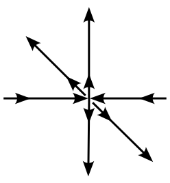
Type B

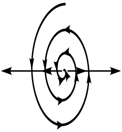
Type As

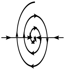
Type Bs

Figure 1: Classification of magnetic nulls – Type A: real eigenvalues with signs (-,-,+); Type B: real eigenvalues with signs (+,+,-); Type As: two complex and one real eigenvalues with signs of real parts (-,-,+); Type Bs: two complex and one real eigenvalues with signs of real parts (+,+,-). Figure from (Franssila, 2023).

2.2 Separatrices and separators

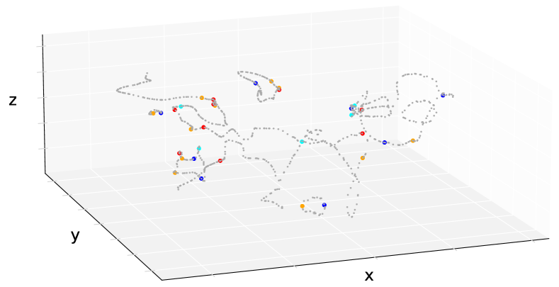
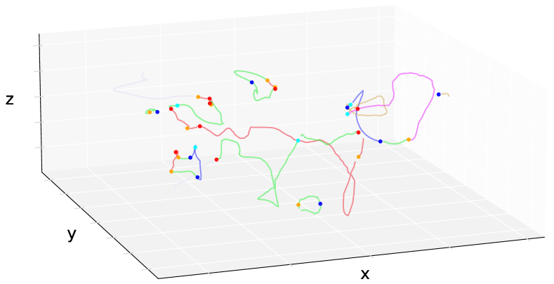
Figure 2: Left: Detected proper and 2D null points. Right: The resulting spatial graph at the same time-step of the simulation. The spatial edges represent different types of separators in blue (As $\leftrightarrow$ Bs), red (A $\leftrightarrow$ B), green (A $\leftrightarrow$ Bs, B $\leftrightarrow$ As), pink (A $\leftrightarrow$ As, B $\leftrightarrow$ Bs) and yellow (A $\leftrightarrow$ A, B $\leftrightarrow$ B, As $\leftrightarrow$ As, Bs $\leftrightarrow$ Bs).

The eigenvectors of the Jacobian can be used to define the so-called separatrices that are associated with the magnetic nulls (Longcope, 2005; Günther & Baeza Rojo, 2020). Each non-degenerate null has one 2D separatrix or fan surface and two one-dimensional virtual separatrices or spines (Longcope, 2005). The fan surface is defined by the infinitely many magnetic field lines within the plane spanned by the two eigenvectors corresponding to the same-sign eigenvalues. The two spine field lines end in the magnetic null point, entering along the directions parallel and antiparallel to the third eigenvector, normal to the fan plane (Longcope, 2005).

In physical simulations, magnetic nulls connect via separator curves (or reconnection lines) formed by the intersection of the fan surfaces of two connected nulls (Palmroth et al., 2006). However, the process of integrating the separatrices to find their intersection can be computationally very expensive, which is why separators are usually approximated (Haynes & Parnell, 2010).

In order to approximate the separators, we choose to follow the 2D null lines: curves along which two of the magnetic field components are zero, while the third can vary. Zeiler et al. (2002) found that with a small guide-field, 3D reconnection is well-approximated by a 2D system. Specifically in the magnetotail environment, we ignore the East-West component of the magnetic field, $B_{y}$, since it tends to exhibit the least variation as the guide-field component, and we require that the other two components are zero, $B_{x}=B_{z}=0$. We call such points 2D nulls and use the term proper null to refer to points where $\|\vec{B}\|_{2}=0$, which are clearly a subset of the 2D nulls. We provide a modification of the existing VTK vector field topology filter to detect such 2D nulls.

3 Graph Representations

Originally introduced by Longcope & Klapper (2002), null graphs are graph representations that characterize the topology of a magnetic field by encoding the connectivity between proper nulls (vertices) via separators (edges).

We extend their definition to construct a graph representation that can be useful for different machine learning tasks and downstream applications, such as spatiotemporal GNNs (Reinhart, 2018). We propose two computationally efficient heuristics to trace the connectivity between proper nulls both spatially and temporally.

3.1 Spatial Null Graphs

After modifying the VTK vector field topology filter to detect the 2D magnetic nulls where $B_{x}=B_{z}=0$ (sec. 2.2), we construct the 2D null lines by connecting the 2D nulls to each other based on spatial proximity.

In practice, the 2D null lines can be traced by initializing at most two paths from each proper null based on a cut-off value on the maximum Euclidean distance from the proper null. Each of the paths is then iteratively expanded by finding – within the same cut-off distance – the nearest 2D null that is not already included in any of the already traced paths. Paths terminating without reaching a proper null are considered a dead end and are discarded, while paths ending at a proper null become edges in the null graph. The type of each proper null (A / B / As / Bs) is encoded as a node feature in the graph.

3.2 Spatiotemporal Null Graphs

Consider a bipartite graph $\mathcal{G}=(\mathcal{V}_{i},\mathcal{V}_{i+1},\mathcal{E})$, where the vertex sets $\mathcal{V}_{i}$ and $\mathcal{V}_{i+1}$ are defined by proper nulls detected at times $t_{i}$ and $t_{i+1}$, respectively. The set of edges $\mathcal{E}$ represents a (partial) matching between the magnetic nulls with the interpretation that vertices $v\in\mathcal{V}_{i}$ and $v^{\prime}\in\mathcal{V}_{i+1}$ are connected by an edge $e=(v,v^{\prime})\in\mathcal{E}$ if they correspond to the same proper null. The problem can be cast as an unbalanced assignment problem defined by the following maximization problem

$$\max_{\mathcal{E}\in\mathfrak{M}}\sum_{(v,v^{\prime})\in\mathcal{E}}1/w(v,v^{\prime}),$$

where the set of allowed matchings $\mathfrak{M}$ is defined by requiring that each vertex appears in at most one edge, and the weight $w(v,v^{\prime})=\|\vec{x}(v)-\vec{x}(v^{\prime})\|_{2}$ is defined by the Euclidean distance between the respective coordinates of the proper nulls $v$ and $v^{\prime}$. Additional constraints including $(i)$ a maximum distance constraint $w_{\max}$, or $(ii)$ matching only the same type nulls, can be incorporated by letting $w(v,v^{\prime})=-1$, for any edge that does not satisfy them. We apply both constraints to get an initial matching, and, for some of the unmatched magnetic nulls, we need to run a subsequent matching without constraint $(ii)$ to account for type switches.

All vertices in $\mathcal{V}_{i}$ that remain unmatched are considered to have disappeared after step $t_{i}$. Likewise, all vertices in $\mathcal{V}_{i+1}$ that remain unmatched are considered to have appeared before step $t_{i+1}$. According to Murphy et al. (2015), proper nulls can either appear by entering the simulation domain across a boundary, or as a result of a bifurcation, in which case they appear in pairs of opposite polarity. These two cases can be distinguished based on the coordinates and types of the unmatched vertices in $\mathcal{V}_{i+1}$.

4 Results and discussion

The supercomputer-generated simulations from Vlasiator provide large-scale, high-fidelity data – some of which is openly available (Palmroth, 2023). To give an idea of the scale of available data, the example of the published Vlasiator dataset provides 170 time-steps $\times$ 1,723,328 grid points at each time-step, i.e., the time series consists of a total of $\sim$ 293 million grid points. Working with such scales requires efficient and scalable methods, and the spatiotemporal graph representation of the data can allow for less resource-intensive machine learning approaches.

The magnetotail simulations used to produce the results presented here, consist of a grid with resolution $50\times 127\times 108$ in the $x$ (tailward–Earthward), $y$ (East–West), and $z$ (North–South) directions of the magnetic field, respectively. A step of one unit in any direction of the grid corresponds to 1000 km, and the time series used to generate the spatiotemporal null graphs has 1 s cadence (Franssila, 2023).

First, the modified VTK topology filter is used to detect 2D and proper nulls, and to classify the latter in types (sec. 2.1). The 2D nulls are detected using $B_{y}$ as the guide-field component (sec. 2.2). The results obtained from the first stage of the process are illustrated on the left side of Figure 2.

The result of the spatial tracing method (sec. 3.1), is presented on the right of Figure 2. The 3D null points are colored according to their type. Different types of spatial connectivity are also color-encoded, using different colors of spatial edges depending on the type of the connection.

Figure 3 shows an example of a spatiotemporal graph, where for each time-step $t_{i}$ for $i\in\{0,1,2\}$, a 2D projection (X-Y plane) of the spatial graph is presented. The temporal edges trace the temporal evolution of each proper null across all time-steps. The colors of the temporal edges represent the type of the proper null traced over time, with the exception of the pink temporal edges which denote a type switch scenario (e.g., $t_{0}\rightarrow t_{1}$: B $\rightarrow$ Bs). Finally, the green circle at $t_{2}$ is used to mark a pair of proper nulls of opposite polarity that appear together before $t_{2}$ due to a bifurcation.

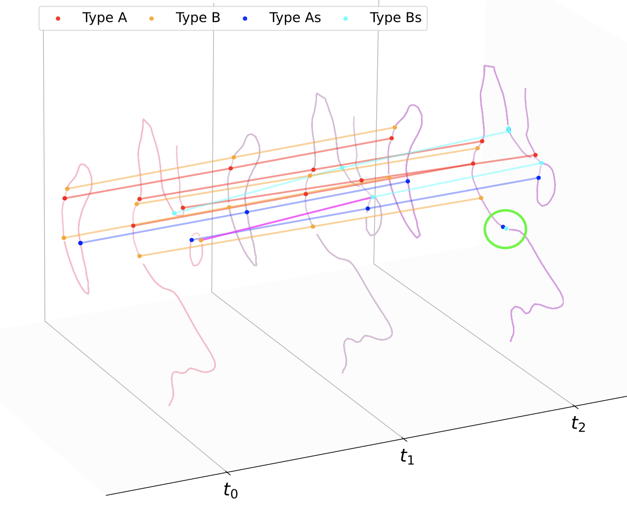
Figure 3: Spatiotemporal null graph. At each time-step a 2D projection (X-Y plane) of the corresponding spatial graph is illustrated. The proper nulls are colored based on their type, and the color of each temporal edge represents the type of the traced proper null, with the exception of the pink edge which denotes a type switch. The green circle at $t_{2}$ marks a pair of proper nulls of opposite polarity that appear together after a bifurcation.

We have presented a scalable data analysis pipeline for the detection and spatiotemporal tracing of proper magnetic nulls. These methods allow us to characterize the topology a 3D magnetic field using graph representations. The resulting spatiotemporal null graphs can be useful in various downstream learning tasks, especially in GNN applications (Reinhart, 2018; Zhou et al., 2020; Wu et al., 2020).

In the process of formulating 3D magnetic reconnection detection as a machine learning task, two potential limitations arise. If we formulate the problem as a supervised learning task, there is a severe difficulty in reliably labeling a sufficient amount of training data, as 3D magnetic reconnection remains difficult to detect and characterize. Similarly, if we were to formulate the problem as an unsupervised learning task, questions arise regarding the interpretability of results and the model performance evaluation.

Currently, we are working on a GNN approach that aims to circumvent these issues by formulating the learning task as a plasmoid formation forecast, as their generation is linked to reconnecting plasmas (Samtaney et al., 2009). The location of a plasmoid can be characterized using the magnetic skeleton (Birn et al., 1997), which allows us to use spatiotemporal null graphs to learn when and where a plasmoid is formed. Next, in order to detect the magnetic reconnection, we can examine the reconnection rate and energy conversion rate at the possible reconnection sites located in close proximity to the newly-formed plasmoid. This work can then be extended to facilitate the study of magnetized plasmas in different settings, which is linked to a variety of open questions that can be interesting to both the astrophysics and machine learning research communities.

References

- Angelopoulos et al. (2008) Angelopoulos, V., McFadden, J. P., Larson, D., Carlson, C. W., Mende, S. B., Frey, H., Phan, T., Sibeck, D. G., Glassmeier, K.-H., Auster, U., et al. Tail Reconnection Triggering Substorm o Onset. Science, 321(5891):931–935, 2008.
- Baker et al. (2004) Baker, D. N., Daly, E., Daglis, I., Kappenman, J. G., and Panasyuk, M. Effects of Space Weather on Technology Infrastructure. Space Weather, 2(2), 2004.
- Birn et al. (1997) Birn, J., Hesse, M., and Schindler, K. Theory of Magnetic Reconnection in Three Dimensions. Advances in Space Research, 19(12):1763–1771, 1997.
- Bujack et al. (2021) Bujack, R., Tsai, K., Morley, S. K., and Bresciani, E. Open Source Vector Field Topology. SoftwareX, 15:100787, 2021.
- Bungey et al. (1996) Bungey, T. N., Titov, V. S., and Priest, E. R. Basic Topological Elements of Coronal Magnetic Fields. Astronomy and Astrophysics, 308:233–247, 1996.
- Cassak & Shay (2007) Cassak, P. A. and Shay, M. A. Scaling of Asymmetric Magnetic Reconnection: General Theory and Collisional Simulations. Physics of Plasmas, 14(10):102114, 2007.
- Daughton et al. (2011) Daughton, W., Roytershteyn, V., Karimabadi, H., Yin, L., Albright, B. J., Bergen, B., and Bowers, K. J. Role of Electron Physics in the Development of Turbulent Magnetic Reconnection in Collisionless Plasmas. Nature Physics, 7(7):539–542, 2011.
- Franssila (2023) Franssila, F. Identifying topological elements of 3D magnetic reconnection. Master’s thesis, University of Helsinki, 2023.
- Günther & Baeza Rojo (2020) Günther, T. and Baeza Rojo, I. Introduction to Vector Field Topology. In Topological Methods in Data Analysis and Visualization VI. Springer, 2020.
- Haynes & Parnell (2010) Haynes, A. and Parnell, C. A Method for Finding Three-dimensional Magnetic Skeletons. Physics of Plasmas, 17(9):092903, 2010.
- Lau & Finn (1990) Lau, Y.-T. and Finn, J. M. Three-dimensional Kinematic Reconnection in the Presence of Field Nulls and Closed Field Lines. The Astrophysical Journal, 350:672–691, 1990.
- Lee (2022) Lee, J. Dimensionality of Solar Magnetic Reconnection. Reviews of Modern Plasma Physics, 6(1):32, 2022.
- Li et al. (2021) Li, T., Priest, E., and Guo, R. Three-dimensional Magnetic Reconnection in Astrophysical Plasmas. Proceedings of the Royal Society A, 477(2249):20200949, 2021.
- Li et al. (2022) Li, X., Wang, R., Lu, Q., Russell, C. T., Lu, S., Cohen, I. J., Ergun, R., and Wang, S. Three-dimensional Network of Filamentary Currents and Super-thermal Electrons during Magnetotail Magnetic Reconnection. Nature Communications, 13(1):3241, 2022.
- Liu et al. (2013) Liu, W., Chen, Q., and Petrosian, V. Plasmoid Ejections and Loop Contractions in an Eruptive M7. 7 Solar Flare: Evidence of Particle Acceleration and Heating in Magnetic Reconnection Outflows. The Astrophysical Journal, 767(2):168, 2013.
- Liu et al. (2022) Liu, Y.-H., Cassak, P., Li, X., Hesse, M., Lin, S.-C., and Genestreti, K. First-principles Theory of the Rate of Magnetic Reconnection in Magnetospheric and Solar Plasmas. Communications Physics, 5(1):97, 2022.
- Longcope (2005) Longcope, D. Topological Methods for the Analysis of Solar Magnetic Fields. Living Reviews in Solar Physics, 2, 2005.
- Longcope & Klapper (2002) Longcope, D. and Klapper, I. A General Theory of Connectivity and Current Sheets in Coronal Magnetic Fields Anchored to Discrete Sources. The Astrophysical Journal, 579(1):468, 2002.
- Ma & Tang (2021) Ma, Y. and Tang, J. Deep Learning on Graphs. Cambridge University Press, 2021.
- Mei et al. (2012) Mei, Z., Shen, C., Wu, N., Lin, J., Murphy, N. A., and Roussev, I. I. Numerical Experiments on Magnetic Reconnection in Solar Flare and Coronal Mass Ejection Current Sheets. Monthly Notices of the Royal Astronomical Society, 425(4):2824–2839, 2012.
- Murphy et al. (2015) Murphy, N. A., Parnell, C. E., and Haynes, A. L. The Appearance, Motion, and Disappearance of Three-dimensional Magnetic Null Points. Physics of Plasmas, 22(10):102117, 2015.
- Odenwald et al. (2006) Odenwald, S., Green, J., and Taylor, W. Forecasting the Impact of an 1859-calibre Superstorm on Satellite Resources. Advances in Space Research, 38(2):280–297, 2006.
- Palmroth (2023) Palmroth, M. Vlasiator 6D EGI Tail Current Sheet Data Series, 2023.
- Palmroth et al. (2006) Palmroth, M., Laitinen, T. V., and Pulkkinen, T. I. Magnetopause Energy and Mass Transfer: Results from a Global MHD Simulation. Annales Geophysicae, 24(12):3467–3480, 2006.
- Palmroth et al. (2017) Palmroth, M., Hoilijoki, S., Juusola, L., Pulkkinen, T. I., Hietala, H., Pfau-Kempf, Y., Ganse, U., Von Alfthan, S., Vainio, R., and Hesse, M. Tail Reconnection in the Global Magnetospheric Context: Vlasiator First Results. Annales Geophysicae, 35(6):1269–1274, 2017.
- Palmroth et al. (2018) Palmroth, M., Ganse, U., Pfau-Kempf, Y., Battarbee, M., Turc, L., Brito, T., Grandin, M., Hoilijoki, S., Sandroos, A., and von Alfthan, S. Vlasov Methods in Space Physics and Astrophysics. Living Reviews in Computational Astrophysics, 4(1):1, 2018.
- Parker (1979) Parker, E. N. Cosmical Magnetic Fields: Their Origin and their Activity. Oxford university press, 1979.
- Parnell et al. (2010) Parnell, C., Haynes, A., and Galsgaard, K. Structure of Magnetic Separators and Separator Reconnection. Journal of Geophysical Research: Space Physics, 115(A2), 2010.
- Priest & Forbes (2000) Priest, E. and Forbes, T. Magnetic Reconnection: MHD Theory and Applications. Cambridge University Press, 2000.
- Priest & Titov (1996) Priest, E. R. and Titov, V. S. Magnetic Reconnection at Three-dimensional Null Points. Philosophical Transactions of the Royal Society of London. Series A: Mathematical, Physical and Engineering Sciences, 354(1721):2951–2992, 1996.
- Pulkkinen et al. (2005) Pulkkinen, A., Lindahl, S., Viljanen, A., and Pirjola, R. Geomagnetic Storm of 29–31 October 2003: Geomagnetically Induced Currents and their Relation to Problems in the Swedish High-voltage Power Transmission System. Space Weather, 3(8), 2005.
- Reinhart (2018) Reinhart, A. A Review of Self-exciting Spatio-temporal Point Processes and their Applications. Statistical Science, 33(3):299–318, 2018.
- Samtaney et al. (2009) Samtaney, R., Loureiro, N., Uzdensky, D., Schekochihin, A., and Cowley, S. Formation of Plasmoid Chains in Magnetic Reconnection. Physical review letters, 103(10):105004, 2009.
- Schroeder et al. (2006) Schroeder, W., Martin, K., Lorensen, B., and Kitware, I. The Visualization Toolkit: An Object-oriented Approach to 3D Graphics. Kitware, 2006.
- Schwenn et al. (2005) Schwenn, R., Dal Lago, A., Huttunen, E., and Gonzalez, W. D. The Association of Coronal Mass Ejections with their Effects near the Earth. Annales Geophysicae, 23(3):1033–1059, 2005.
- Taylor (1986) Taylor, J. Relaxation and Magnetic Reconnection in Plasmas. Reviews of Modern Physics, 58(3):741, 1986.
- Wu et al. (2020) Wu, Z., Pan, S., Chen, F., Long, G., Zhang, C., and Philip, S. Y. A Comprehensive Survey on Graph Neural Networks. IEEE transactions on neural networks and learning systems, 32(1):4–24, 2020.
- Yamada (1999) Yamada, M. Review of Controlled Laboratory Experiments on Physics of Magnetic Reconnection. Journal of Geophysical Research: Space Physics, 104(A7):14529–14541, 1999.
- Yamada et al. (2010) Yamada, M., Kulsrud, R., and Ji, H. Magnetic Reconnection. Reviews of modern physics, 82(1):603, 2010.
- Zeiler et al. (2002) Zeiler, A., Biskamp, D., Drake, J., Rogers, B., Shay, M., and Scholer, M. Three-dimensional Particle Simulations of Collisionless Magnetic Reconnection. Journal of Geophysical Research: Space Physics, 107(A9):SMP–6, 2002.
- Zhou et al. (2020) Zhou, J., Cui, G., Hu, S., Zhang, Z., Yang, C., Liu, Z., Wang, L., Li, C., and Sun, M. Graph Neural Networks: A Review of Methods and Applications. AI open, 1:57–81, 2020.