A Cryogenic Memristive Neural Decoder
for Fault-tolerant Quantum Error Correction

Abstract

Neural decoders for quantum error correction (QEC) rely on neural networks to classify syndromes extracted from error correction codes and find appropriate recovery operators to protect logical information against errors. Despite the good performance of neural decoders, important practical requirements remain to be achieved, such as minimizing the decoding time to meet typical rates of syndrome generation in repeated error correction schemes, and ensuring the scalability of the decoding approach as the code distance increases. Designing a dedicated integrated circuit to perform the decoding task in co-integration with a quantum processor appears necessary to reach these decoding time and scalability requirements, as routing signals in and out of a cryogenic environment to be processed externally leads to unnecessary delays and an eventual wiring bottleneck. In this work, we report the design and performance analysis of a neural decoder inference accelerator based on an in-memory computing (IMC) architecture, where crossbar arrays of resistive memory devices are employed to both store the synaptic weights of the decoder neural network and perform analog matrix–vector multiplications during inference. In proof-of-concept numerical experiments supported by experimental measurements, we investigate the impact of TiO_x-based memristive devices’ non-idealities on decoding accuracy. Hardware-aware training methods are developed to mitigate the loss in accuracy, allowing the memristive neural decoders to achieve a pseudo-threshold of $9.23\text{\times}{10}^{-4}$ for the distance-three surface code, whereas the equivalent digital neural decoder achieves a pseudo-threshold of $1.01\text{\times}{10}^{-3}$. This work provides a pathway to scalable, fast, and low-power cryogenic IMC hardware for integrated QEC.

Introduction

Fault-tolerant quantum computation (FTQC) holds the promise of solving extremely difficult problems with efficient time and space complexity [1, 2]. However, this efficiency is at the cost of resource-intensive classical procedures that are required for protecting the logical quantum state of the quantum processor against noise [3]. This includes, (a) thermal processes to physically protect the quantum state by cooling and isolating the quantum processor, and (b) computational processes for executing quantum control protocols and performing quantum error correction. The former is the reason many quantum technologies use cryogenic temperatures. But, the latter requires classical computers that have historically been designed and manufactured to operate at room temperature and their high heat dissipations hinders their use inside cryostats. With microsecond-long error correction cycles, FTQC with the anticipated needed millions of physical qubits (or more) will produce at least hundreds of gigabytes of syndrome data per second which have to be transferred from the cold measurement environment to the room temperature electronics and this process is expected to last at least for hours, if not days, for each run of a useful quantum algorithm [2]. Transferring and processing this amount of data is a nontrivial task even for powerful classical computing centres, but the challenge is exacerbated by additional requirements for FTQC: (i) quantum measurements produce weak signals that have to amplified in multiple rounds in order for them to be transferred to room temperature electronics, and (ii) FTQC implementation of non-Clifford gates require active error correction and therefore this large amount of data has to be processes in real-time and the resulting recovery operations have to be applied at a time scale comparable to the coherence time of the quantum sytem [4, 5].

Classical processors that can operate at the unfriendly cryogenic environments can overcome the above challenges. This requires rethinking classical computing technologies (e.g., CPUs, GPUs, and FPGAs) and building processors that can operate at extremely low power consumptions, in order to avoid heat dissipation from the classical processes of FTQC as the cooling power of cryostats is often limited to a few milliwatts. As a result, several research groups in quantum information processing are engaged in developing cryogenic quantum controllers using integerated CMOS [6, 7, 8], single flux quantum (SFQ) [9, 10, 11], and even resistive memory technologies [12]. In contrast, cryogenic decoders have not been as well studied. References [13, 14, 15] propose SFQ-based architectures for decoding using various heuristic approximations to graph matching algorithms, whilte [16] proposes a binarized SFQ-based neural decoders.

The main challenge in building cryogenic scalable fault-tolerant decoders is its need for high-density cryogenic memory blocks. There are at least two types of memory blocks required for the decoder.

1. The ‘program’ data: Even the simplest decoding heuristics are quite complicated computations for edge computation at extreme cryogenic conditions. Therefore they must rely on various look-up tables (e.g., for edge and vertex weights in graph-based decoders [17, 18, 19]).

2. The ‘syndrome’ history (the input data): Since fault-tolerant error correction requires processing of multiple rounds of imperfect measurements (typically as a graph-based algorithm on a 3-dimensional lattice), the behaviour of the decoding algorithm depends on historical values of the syndrome bits and therefore some type of memory must store and recall this information.

In this paper, we introduce a memristive neural decoders (MND) which combines the advantages of recurrent neural networks (RNN) and the low-power consumption of resistive memory arrays to eliminate the need for both types of cryogenic memory blocks. In the case of deep neural decoders, the ‘program’ data is the weights and biases of a neural network [20]. This information is stored in the conductance states of the resistive memory devices which are physically tuned, thereby providing a realization of in-memory computation (IMC) [21]. In addition, an RNN comprises an internal state which is a real-valued vector (or perhaps a higher-dimensional tensor) that encodes features of historical data (the $h$ wires Fig. 1). The RNN will therefore not require to receive the syndrome data of multiple rounds of error correction at once, and instead processes them one at a time, while updating its internal state in each iteration (from $h_{i}$ to $h_{i+1}$ in Fig. 1).

More specifically, we investigate TiO_x-based analog resistive memory devices using TiN electrodes [22]. A crossbar arrangement of these memory cells enables the matrix–vector multiplication (MVM) operations at the heart of neural network algorithms to be performed natively by relying on Ohm’s law and Kirchoff’s circuit law, thus removing the time- and energy-intensive process of shuffling data from memory to processing units [23]. Such memristive devices [24, 25, 26, 27] are non-volatile, making them promising candidates for ultra-efficient MVM, in terms of processing time, energy dissipation, and scalability [28]. Furthermore, they have recently been shown to operate at cryogenic temperatures [29, 30] and their fabrication process is CMOS compatible [22]. Memristive devices have better footprints compared to the alternative CMOS-based static random access memory (SRAM) which have also been proposed for IMC neural decoding [31]. A similar apporoach is demonstrated in [32] using binary resistive random access memory (RRAM). We note that both [31] and [33] rely on LSTM units which are much more complex neural networks than the simple RNN we train in this paper for the same task [34].

We leave a detailed analysis of the energy consumption of our device to future publications, and in this paper focus on the non-idealities of resistive memory arrays which are known to deteriorate neural networks’ precision [35]. We therefore simulate the impact of key TiO_x-based resistive memory devices’ non-idealities on the accuracy of the MND and apply hardware-aware training techniques in order to avoid performance decay. We use a distance $3$ rotated surface code as our case study, and note that RNN-based decoders can be trained for other error correcting codes as well [20]. We demonstrate that hardware-aware training can enable high-accuracy classification of surface code syndromes with an MND and provide an engineering approach for improving processing time and energy consumption of decoding circuitry with analog resistive memory modules.

This paper is structured as follows. First, we provide a formal definition of the decoding problem, describe the decoder neural network’s architecture and present the memristive decoder circuit. Next, we characterize key hardware non-idealities on resistive memory devices. We then apply hardware-aware training methods and recover near maximal classification accuracy for the memristive decoder despite TiO_x-based resistive memory devices’ non-idealities. Finally, we discuss the engineering advantages of leveraging analog IMC hardware for decoding in the context of QEC.

Problem Statement

Decoding the surface code

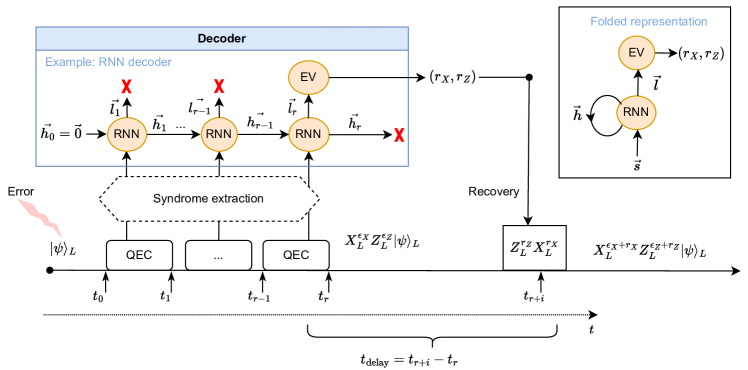
Figure 1: Decoding process. In quantum error correction (QEC), syndrome extraction rounds are performed cyclically to protect an encoded quantum state $\ket{\psi}_{L}$ from logical errors. Typically, the $X$ and $Z$ stabilizers’ syndromes are processed separately but simultaneously by two independent decoding modules. The syndrome measurement outcomes are fed to the decoder modules, which analyze them to produce a decision output $(r_{X},r_{Z})$. This decision output is used to construct the recovery operation $Z_{L}^{r_{Z}}X_{L}^{r_{X}}$. Between the end of the last QEC round at $t_{r}$ and the application of the recovery operation at $t_{r+i}$, idling errors can affect the qubits, and they will not be taken into account by the decoding algorithm. The encoded state just prior to the application of recovery operations is therefore $X_{L}^{\epsilon_{X}}Z_{L}^{\epsilon_{Z}}\ket{\psi}_{L}$, where $\epsilon_{x,z}$ represent the cumulative effect of the errors that occurred during the QEC rounds and the idling time $t_{\textrm{delay}}$. Following the application of the recovery operation (here assumed to be ideal for simplicity), the final encoded logical quantum state is $X_{L}^{\epsilon_{X}+r_{X}}Z_{L}^{\epsilon_{Z}+r_{Z}}\ket{\psi}_{L}$. Here, the illustrative decoder is based on a recurrent neural network (RNN). Each new syndrome is used as the input to the RNN and the hidden state $\vec{h_{i}}$ is passed to the subsequent recurrence. At the end of the QEC process, the output state $\vec{l_{r}}$ is passed to an evaluation module EV, typically a feedforward NN, to provide the final binary output of the decoder. On the right-hand side of the figure, the standard folded representation of this RNN is illustrated, in constrast with the unfolded representation on the left-hand side. The more detailed schematic architecture of this RNN decoder is depicted in Fig. 3.

Given a logical quantum state $\ket{\psi}_{L}$ encoded by a quantum error correcting code, the process of active error correction via stabilizer meaurements and decoding is schematized in Fig. 1. Successful error correction amounts to matching the decoder-proposed recovery operator $(r_{X},r_{Z})$ with the actual logical error $(\epsilon_{X},\epsilon_{Z})$ afflicting the state $\ket{\psi}_{L}$. Indeed, the speed and accuracy of a decoder are interconnected, due to idling errors associated with the decoding delay. As a rule of thumb, minimizing the decoding time as much as possible is desirable.

We consider the distance-three rotated surface code, which can be realized with 17 physical qubits [36, 37, 38]. As shown in Fig. 2(a), the qubits are arranged on a square lattice, comprising data qubits (circles filled in white) and ancilla or syndrome qubits (circles filled in black). Data and syndrome qubits differ only in terms of their function within the code, and they can be implemented using physical systems such as superconducting circuits, trapped ions, quantum dots, or topological qubits. Each qubit interacts with its neighbours in a specified manner. The order and mechanism of interaction is determined by the stabilizers being measured, as shown in Fig. 2(b) and (c) for stabilizers $X_{e}X_{f}X_{g}X_{h}$ and $Z_{a}Z_{b}Z_{c}Z_{d}$, respectively.

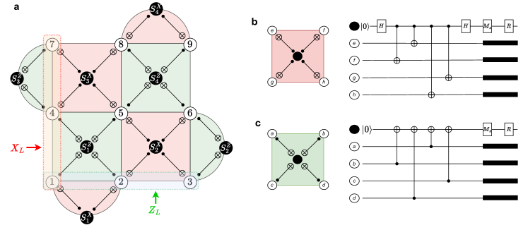
Figure 2: Surface code and stabilizer measurements. (a) Distance-three rotated surface code, also called surface-17. Data qubits 1 to 9 are identified by circles filled in white, and syndrome qubits are identified by circles filled in black. Each syndrome qubit resides on a “plaquette” corresponding to a specific stabilizer measurement $S$. The sequence of operations realizing an $X$ stabilizer (pink plaquette) and a $Z$ stabilizer (green plaquette) are shown in (b) and (c). In this example, a logical operator $X_{L}$ ($Z_{L}$) can be realized by applying a chain of physical $X$ ($Z$) operators on data qubits between the top (left) and bottom (right) edge of the grid. (b) Sequence of circuit operations between a syndrome qubit (circle filled in black, the top qubit in the circuit) and its neighbouring data qubits, $e$, $f$, $g$, and $h$, realizing the stabilizer measurement $X_{e}X_{f}X_{g}X_{h}$. It consists of syndrome qubit initialization, Hadamard gates (H), CNOT gates, a projective measurement along the z-axis ($M_{Z}$), and a reset ($R$) to the $\ket{0}$ state, regardless of the measured outcome. (c) Sequence of circuit operations between a syndrome qubit and its neighbouring data qubits, $a$, $b$, $c$, and $d$, realizing the stabilizer measurement $Z_{a}Z_{b}Z_{c}Z_{d}$. It consists of syndrome qubit initialization, CNOT gates, and a projective measurement along the z-axis. The black rectangles represent idling of the data qubits, which is important for simulation of the circuits. More details on the exact procedure used for the simulation of those parity-check circuits is provided in Supplementary Note 1.

Neural decoder architecture

We consider an RNN decoder module similar to the ones described in Refs. [20] and [39]. It may be difficult to train neural decoders for arbitrarily large topological codes, however we note that the largest topological patch that must be actively decoded during FTQC depends on the largest entangling gate between a logical magic state and other logical qubits [40]. Additionally, neural decoders are great candidates for inclusion in distributed [41] and heirarchical decoding schemes [42] in order to achieve larger scale decoding systems. We restrict our numerical benchmarks to the $X$ syndromes since the performance would be the same for the $Z$ syndromes. Supplementary Note 1 describes the model used to simulate the quantum circuit and obtain the syndromes data sets and labels for training of the RNN decoder.

Our RNN architecture is illustrated in Fig. 3(b). It consists of a fully connected recurrent layer, and a fully connected evaluation layer. There are four input nodes for receiving the syndrome data of an error correction round and four internal state nodes that are connected to the outputs nodes of the recurrent layer. Assuming similar error rates for physical gates and measurement, the distance-three code requires three QEC cycles to be fault tolerant [43, 20, 39]. The outputs of the recurrent layer, after application of the activation function (here we use ReLU) are fed back to the internal state nodes as the next error correction round syndrome data ($s^{X}$) arrives to the input nodes, and this is repeated for a total of at least three cycles, as illustrated in Fig. 3(a). In order to evaluate the logical error rate of the scheme, we measure the data qubits in a final (fourth) cycle which we call the perfect syndrome extraction round or the “perfect round” for short (see Supplementary Note 1).

After the fourth round has been provided as input to the input nodes, the output of the recurrent layer is forwarded to the evaluation layer and passed through a Max function. Subsequently, the neural decoder outputs a single binary result, 0 or 1, indicating whether a logical error has occurred at the end of the QEC rounds (Fig. 3(d)). We note that in general for multi-label classification the number of output nodes are the same as the number of classes, which is what we used. However since the decoder problem is a binary classification, one output node would suffice.

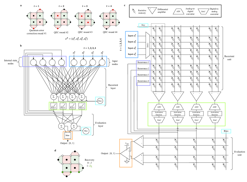
Figure 3: Recurrent neural network decoder architecture and corresponding memristive decoder circuit. Quantum error correction is handled as a sequential classification problem. (a) Error correction (EC) rounds are performed by measuring stabilizer operators on the lattice of physical qubits. Ancilla qubits (the circles filled in red or black representing an error or no error being detected, respectively) measure the bit-flip $X$ (phase-flip $Z$) stabilizers $\hat{S}_{\{1-4\}}^{X}$ ($\hat{S}_{\{1-4\}}^{Z}$). Measured eigenvalues of ancillas are mapped to classical bits to build the syndromes $s^{X}$ and $s^{Z}$, which serve as inputs to the neural decoder. Here, we consider only the $s^{X}$ syndromes, obtained at times $t=1,2,3,4$. (b) Recurrent neural network decoder architecture for the distance-three surface code. It comprises a recurrent layer and an evaluation layer. Bias are also applied to the output nodes of the recurrent and evaluation layers. The syndrome at $t=1$ is the initial input along with the initialized hidden state $\vec{h_{0}}$. The output of the recurrent layer is routed back to the internal state nodes, as a new syndrome ($t=2$) is provided to the input nodes. This is repeated until the last EC round at time $t=n$ (here, $n=4$), when the output of the recurrent layer is forwarded to the evaluation layer, where the values of the two output neurons are passed through a Max function to produce a binary classification. (c) Memristive decoder circuit. It is composed of two tiles of resistive memory devices. The first is applied recursively (recurrent unit) until $t=n$, and the second acts as the classifier (evaluation unit). Input syndromes are converted from the digital domain to the analog domain by DACs so that the memristive crossbar can perform the analog MVM. The resistive memory devices’ conductances are programmed according to the (numerically) trained weights of the equivalent neural network decoder. Differential amplifiers subtract the outputs from each pair of resistive memory columns to obtain the resulting node value. This signal is forwarded to the activation function unit (green rectangle), where an analog-to-digital conversion is performed to apply a numerical activation function (ReLU). The signal is converted back to the analog domain before being routed back to the recurrence input ports or sent to the evaluation unit. Finally, the outputs of the evaluation unit are passed through a comparator to produce a binary classification. An additional resistive memory row in each unit allows the application of a bias signal. (d) To conclude the error correction process, a recovery operation is applied to the data qubits according to the classification provided by the decoder. The identity is applied in the case where no logical error has been detected (output 0), and the $Z_{L}$ operator is applied (circles filled in green) if a logical error has been detected (output 1).

Memristive neural decoder

We present a memristive electronic circuit to implement the neural decoder architecture discussed above, where the parameters of the neural network are stored in crossbar arrays of TiO_x resistive memory. The memristive neural decoder (MND) architecture is shown in Fig. 3(c). It comprises two distinct resistive memory arrays, also called units: the recurrent unit, which maps the weights corresponding to the recurrent layer, and the evaluation unit, which maps the weights corresponding to the evaluation layer [44], in accordance with the architecture shown in Fig. 3(b). Between the two crossbars of memristive devices, we perform an analog-to-digital conversion to apply a numerical activation function. The output is then converted back into an analog signal, for example, in the form of a voltage pulse. Performing this step in the digital domain simplifies the circuit design by removing concerns about analog signal deterioration, as it offers full control over the shape of the signal sent into the second layer. The range and resolution of analog-to-digital converters (ADC) and digital-to-analog converters (DAC) is further discussed in Supplementary Information Note 2.

Input ports receive data from syndrome measurements in the form of electronic signals, which could be encoded in, for example, voltage pulse durations [28] or pulse amplitudes [45]. Recurrence ports receive the routed-back, updated output from the recurrent unit at each cycle. Finally, the output port provides the binary classification result of the decoder, which determines the recovery operation to be applied to the surface code.

We present now in greater detail the operation of the resistive memory crossbar arrays needed to perform analog MVM. The memristive device consists of two TiN electrodes separated by a TiO_x-based switching layer [22]. Following an initial non-reversible electroforming process, a conductive filament containing oxygen vacancies is created within the oxide layer [46], which can be subsequently at least partially dissolved and re-established through voltage pulses on the electrodes, leading to programmable, non-volatile conductance states for the memristive device [47].

It is therefore possible to map the weights $W_{jk}$ of a neural network layer into the conductance states $G_{jk}^{\pm}$ of resistive memory devices. To implement both positive and negative weights, the following mapping is used:

$$G_{jk}^{\pm}=|W_{jk}|\frac{G_{\textrm{HCS}}-G_{\textrm{LCS}}}{W_{\textrm{max}}}+G_{\textrm{LCS}},$$ (1)

where $W_{\textrm{max}}$ is the absolute maximum weight of a given layer, and $G_{\textrm{HCS}}$ and $G_{\textrm{LCS}}$ are the conductance values of the highest and lowest conductance states, respectively. That is, they are the maximum and minimum values that can be programmed on the TiO_x device. If $W_{jk}>0$, $G_{jk}^{+}$ is programmed with respect to Eq. (1) and $G_{jk}^{-}$ is set to $G_{\textrm{LCS}}$. If $W_{jk}<0$, $G_{jk}^{-}$ is programmed with respect to Eq. (1) and $G_{jk}^{+}$ is set to $G_{\textrm{LCS}}$. The network is trained using software with specific computational methods, as we discuss in the Results section, after which the trained weights can be mapped to conductances.

A crossbar configuration allows memristive devices to realize MVM natively, by relying on Ohm’s law and Kirchoff’s circuit laws. In Fig. 3, the current output of each column $C_{k}$ in the crossbar array is the sum of the input rows’ voltages multiplied by the effective conductance values of the differential pairs of memristive devices. From the circuit laws, we have

$$i_{k}=\sum_{j}\left(G_{jk}^{+}-G_{jk}^{-}\right)v_{j},$$ (2)

where $i$, $v$, and $G$ respectively denote current, voltage, and conductance, and $j$ and $k$ are the indices for rows and columns, respectively. For each differential amplifier, the superscripts $+$ and $-$ denote the polarity of the pins wired to the resistive memory devices. From Eq. (2), each column implements naturally the multiply-accumulate (MAC) operation [48].

Results

In this section, we describe and experimentally characterize various hardware non-idealities of TiO_x devices. We then simulate the impact of those key non-idealities on the accuracy of the MND, and demonstrate mitigation strategies using hardware-aware training methods.

Characterization of non-idealities of TiO_x resistive memory devices

From their stochastic nature, oxide-based resistive memory devices exhibit multiple non-idealities [49, 50, 51, 52] such as programming variability and stuck-at fault devices. These non-idealities are expected to decrease the accuracy of a memristive neural decoder with respect to its digital equivalent.

Programming variability is responsible for the inaccurate mapping of the trained weights to the conductance states of resistive memory devices. The conductance states are programmed using a closed-loop read–write–verify algorithm [47] (see Supplementary Note 3), as presented in Fig. 4 (a). However, the target values given by Eq. (1) are never reached exactly. A programming variability model [30] that actually accounts for cycle-to-cycle variability (variation between instances of programmed values on the same device for the same target conductance) and device-to-device variability (variation between programmed values on nominally identical devices for the same target conductance) has been obtained from experimental characterizations of TiO_x memory devices. The characterization process is detailed in Supplementary Note 3. Therefore, the actual programmed values are expected to be

$$G_{jk}^{\pm}\leftarrow G_{jk}^{\pm}+\mathcal{N}(0,\sigma_{\text{prog}}(G_{jk}^{\pm})),$$ (3)

where $\sigma_{\text{prog}}(G_{jk}^{\pm})$ follows the polynomial fit of Fig. 4(b). The median value of the relative variations, that is, $\sigma_{\text{prog}}(G_{jk}^{\pm})/G_{jk}^{\pm}$, reported in Fig. 4(b) is $0.8\%$ for TiO_x devices in the conductance range [60, 200] $\text{\,}\mathrm{\SIUnitSymbolMicro S}$. In comparison, a median value of $3.8\%$ has been reported for phase-change memory (PCM) devices from a similar experiment in a lower conductance range [35], which is expected to exhibit less programming variability.

The yield of functional devices on a chip is not perfect from the nanofabrication process. This translates into a certain probability of stuck-at fault devices, that is, memory devices stuck in either HCS or LCS after electroforming or shortly after a conductance programming attempt [53]. In this case, it cannot be programmed to the desired value for mapping a given weight of the neural network. Note that recent work on passive crossbars of resistive memory have shown a probability of stuck-at fault devices in the order of $\sim$1% [54, 55, 56]. In the case of our specific TiO_x-based memory devices, this probability can reach $\sim$10% and the devices are usually stuck in HCS.

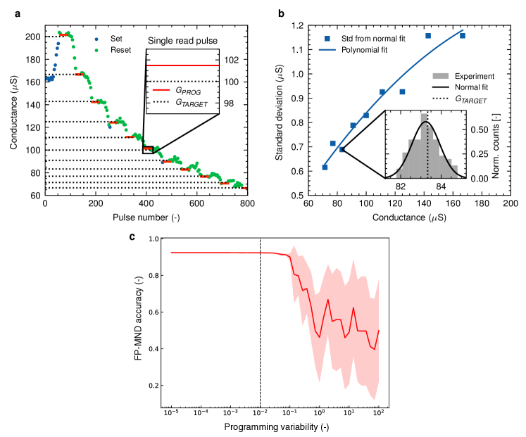
Figure 4: Programming variability characterizations of TiO_x resistive memory. (a) Pulse programming of 11 conductance states of a TiO_x resistive memory device. Positive voltage pulses induce a conductance increase (Set) due to the growth of the conductive filament inside the TiO_x layer between the electrodes. Negative voltage pulses are employed to decrease the conductance (Reset) due to the dissolution of the conductive filament. The dashed black lines denote the target conductances, whereas the solid red lines denote the programmed conductances upon convergence of the closed-loop read–write–verify algorithm. The inset shows the error between target and programmed values for one conductance state. Note that a single read pulse is applied to read the programmed conductance, although it is represented on multiple pulse numbers to ensure visibility. (b) Programming variability model based on the standard deviations in programming errors of multiple conductance states. The multilevel programming cycle shown in (a) is repeated 10 times in a double sweep for 10 devices. For each conductance state, the standard deviation of the programmed values’ distribution is extracted to fit a programming variability model. (c) Accuracy of the FP-MND for different programming variabilities. The vertical line represents a $1\%$ variability. Beyond a $10\%$ variability, the accuracy drops significantly.

Hardware-aware training

From the hardware non-idealities characterized in the previous section, it is expected that the mapping of numerically trained weights to resistive memory conductances would decrease the accuracy of the neural decoder. Therefore, we investigate retraining methods to improve the accuracy of the memristive neural decoder. Hardware-aware (HWA) training refers to the implementation during neural network retraining of specific techniques based on statistical experimental data of the envisioned hardware’s non-idealities. The objective is to make the final model more robust against those non-idealities during inference [57]. The general idea is to fine-tune a conventional digital neural decoder referred to as the baseline. Supplementary Note 4 provides details about the implementation of training and inference in our experiments.

We evaluate the necessity of implementing a specific training method to compensate for the programming variability of 0.8$\%$ observed in our TiO_x memristive devices (Fig. 4(b)) by investigating its impact on the accuracy of the neural decoder. Fig. 4(c)) shows no significant drop in accuracy below 10$\%$ variability. Therefore, beyond injection of Gaussian noise to the weights during retraining [58, 59], which has been shown to improve the accuracy of a memristive neural network [35], we do not consider any novel hardware-aware training method related to programming variability.

We then perform parametric studies to investigate the impact of stuck-at fault devices on the neural decoder’s accuracy. To emulate this non-ideality, a random set of digital weights is set to zero during inference. This situation corresponds to the case where one of the memristive devices of a differential pair is stuck in the HCS and the other is either also stuck or purposefully programmed in the HCS in order to bring the analog weight to 0. The results presented in Fig. 5(a) (blue curve) show that a drop in accuracy of more than $20\%$ can be expected when the percentage of stuck-at fault parameters during inference reaches $20\%$. To mitigate this significant loss in accuracy, we implement random dropping of connections during retraining to increase the robustness of the model against stuck-at fault devices. This regularization technique, also called dropconnect, is typically used to avoid overfitting on the training dataset [60]. In comparison to dropout [61], dropconnect sets weights instead of activations to zero during the forward pass. In that sense, it is well-suited to account for stuck-at fault devices since a differential pair of resistive memory devices, where one is stuck in the high-conductance state and the other one is either also stuck or left in the high-conductance state, would result in an effective weight close to zero. The accuracy of the MND, retrained with different probabilities of random dropconnect $p_{\text{drop}}$, is shown in Fig. 5(a), as a function of the percentages of stuck-at fault parameters.

The accuracy globally improves when dropconnect are introduced during retraining compared to the case where no dropconnect is employed (blue curve). It also appears that to get the best accuracy, the value of $p_{\text{drop}}$ has to be close to the percentage of stuck-at-fault parameters, especially as this percentage increases. Therefore the optmized $p_{\text{drop}}$ value would be approximately equal to the stuck-at-fault parameters percentage.

Dropping connections randomly during retraining provides a generic mitigation strategy applicable to any memristive crossbar architecture given knowledge of the average stuck-at-fault rate is available. However, it does not allow recovery of an accuracy close to baseline even for low rates of stuck-at fault devices. Therefore, we study a more specific retraining scheme where the connections corresponding to the actual location of stuck-at fault parameters in a specificcally characterized crossbar are dropped. Beyond preventing the mapping of large weights to stuck-at fault parameters [62], this scheme entirely prevents updates of weights that cannot be reliably programmed in the crossbar. The idea of this device-specific retraining is to leverage precise hardware knowledge to find the best network parameters for that circuit. It has the advantage of converging towards an optimized solution as we show below, at the cost of individually characterizing each crossbar of the memristive neural decoder to localize stuck-at-fault devices, which can be achieved through methods such as march tests [63, 64].

Figure 5(b) compares for different rates of stuck-at fault parameters the accuracy of different versions of the neural decoder:

• The baseline decoder is purely digital and doesn’t include non-idealities during inference;

• The FP-MND includes the experimentally characterized programming variability during inference, and assumes a finite 8-bit input-output resolution.

• The HWA-MND also includes those non-idealities, but is retrained using random dropconnects with an optimized $p_{\text{drop}}$, as well as a $0.8\%$ Gaussian noise injection.

• The DS-MND also includes those non-idealities, but uses device specific dropconnect retraining and a $0.8\%$ Gaussian noise injection.

The results indicate that only device-specific (DS) retraining allows the drop in accuracy to remain below $1\%$ with respect to the baseline accuracy, even with a $20\%$ rate of stuck-at fault parameters. Interestingly, for the FP-MND, the high standard deviation on the accuracy originating from the programming variability can cause the maximum accuracy of 0$\%$ stuck-at fault parameters to be higher than the baseline. For the MNDs accounting for the programming variability during training (HWA and DS), the smaller standard deviation stems from more-robust models.

Fig. 5(c) represents the decoding performance of the MNDs studied in Fig. 5(b) for different physical fault rates (PFR) and for a percentage of stuck-at fault parameters of $10\%$. Only the DS retraining scheme maintains the pseudo-threshold of the memristive decoder near the pseudo-threshold of the baseline decoder. Therefore, based on the characterized non-idealities in TiO_x memristive devices, it is a necessity to introduce specific knowledge of the chip during retraining to preserve decoding performance. The general solution provided by HWA retraining (random dropconnect) is insufficient. The test accuracy at a PFR of $10^{-2}$ is represented in a histogram in Fig. 5(d) to clearly gauge the performance differences between the training schemes. Floating-point training of the memristive decoder considerably degrades its accuracy, with a nearly $20\%$ drop with respect to baseline accuracy. Hardware-aware training mitigates non-idealities, but the accuracy drop is still $>5\%$. Device-specific retraining significantly improves the performance of the memristive decoder, with an accuracy drop of $<1\%$ with respect to the baseline.

Other HWA training methods for the memristive neural decoder are described in Supplementary Information Note 4, such as input/output discretization and weights clipping. We find that these additional methods are less beneficial than dropconnect for mitigating the characterized non-idealities in TiO_x memristive devices.

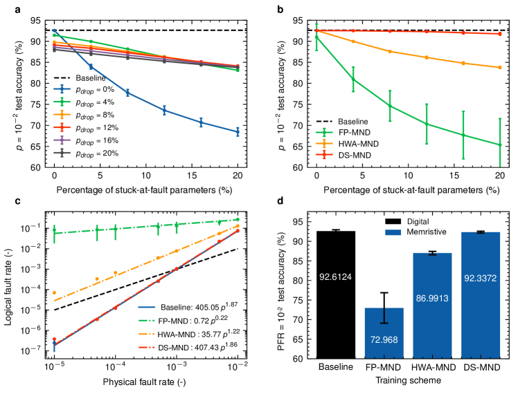
Figure 5: Hardware-aware training methods for the memristive neural decoder. (a) Test accuracy at a physical fault rate(PFR) of $10^{-2}$, for different dropconnect probabilities ($p_{\text{drop}}$) during retraining, as a function of the percentage of stuck-at fault parameters during inference. (b) Test accuracy at a PFR of $10^{-2}$, for different training schemes, as a function of the percentage of stuck-at fault parameters. (c) Logical fault rate after decoding as a function of the PFR in the circuit-level noise model. For each type of training, a monomial fit $ap^{b}$ is performed, where $p$ is the physical fault rate. The values for $a$ and $b$ are shown in the legend. (d) Test accuracy at a PFR of $10^{-2}$ for the different training schemes. In (a), (b), (c), and (d), the baseline accuracy is obtained with the equivalent digital neural decoder, and the error bars are obtained from 100 inference runs averaged over 10 training runs. The labels stand for floating-point training (FP), hardware-aware retraining (HWA), device-specific retraining (DS), and memristive neural decoder (MND).

Discussion

In this work, we have introduced the concept of an RNN decoder relying on the IMC paradigm to perform MVM on passive crossbars of TiO_x-based resistive memory devices. We developed a simulation framework accounting for the experimentally characterized non-idealities of TiO_x-based resistive memory devices and measured their impact on the neural decoder’s performance. By applying computational methods to mitigate key hardware non-idealities, we improved the robustness of the neural decoder. In particular, we found that introducing dropconnect during retraining can greatly improve the accuracy of a memristive neural decoder that suffers from stuck-at fault devices. Moreover, we have seen that localizing stuck-at fault memory devices in the crossbars and using that knowledge to disable the corresponding connections during numerical training can lead to an accuracy very close ($<1\%$ diminution) to that of the baseline digital neural network. Furthermore, our memristive neural decoder shows only a small drop of the pseudo-threshold (from $1.01\text{\times}{10}^{-3}$ to $9.23\text{\times}{10}^{-4}$) for the distance-three surface code in numerical simulations. Therefore, our results supports the effectiveness of specialized training methods in memristive neural decoders for achieving near-optimal performance.

The main advantage of the memristive neural decoder presented in this work is that, in terms of energy, there are no expensive digital units such as multipliers and adders required to perform MVM. On the other hand, whereas hardware implementations of neural networks using ASICs and FPGAs are optimized in comparison to CPU-based approaches, they still suffer from the delays and energy expenditure associated with digital MAC operations. Furthermore, even in recently proposed approaches introducing the idea of quantized IMC for quantum error correction [31, 32], the implementations still require digital multipliers and adders.

Although our proof-of-concept experiment is not performed on fully integrated memristive IMC hardware, the results we have presented offer a promising pathway to realizing highly performant neural decoders using IMC and analog memristive devices. One interesting avenue of research is the development of a fully analog version of the memristive decoder circuit presented herein. Such an implementation would bring further benefits in terms of energy efficiency and processing time of the decoder. We note that analog activation functions have been recently reported in the literature. For instance, ReLU can be applied in the analog domain using multimodal transistors [65]. One could therefore envision disposing of ADCs/DACs. A practical circuit would also necessitate many more electronic components to realistically perform the decoding task, some of which we did not consider here. For example, transimpedance amplifiers (TIA) would be needed to convert the current signals at the output of a resistive memory row to a voltage signal. Also, a type of analog memory unit might be necessary to store and transmit the hidden state signals back to the recurrence input ports.

In our work, we made the assumption that imperfections arising from analog or digital CMOS components (noise introduced by differential amplifiers, TIAs and ADCs/DACs, divergence of the analog activation function from ideal/numerical version in the case of a fully analog implementation, signal distortion arising from multiple recurrences, etc.) are much less critical for the memristive neural decoder’s accuracy in comparison to the non-idealities exhibited by the resistive memory devices. However, future work should include a more exhaustive analysis of the impact of circuit-level imperfections. Previous studies have introduced circuit-level variations in training methodology [66, 67].

Scalability is a concern for QEC decoders, and neural decoders are no exception. As the error correction code distance increases, the syndrome space grows exponentially. Neural decoders thus require an exponentially larger dataset to learn the pattern between syndromes and the occurrences of logical errors. Alone, our proposed approach does not overcome this issue. However, it can be integrated in a multi-stage or hierarchical decoding scheme [41, 68, 69]. Multi-stage or hierarchical approaches have been proposed to improve the efficiency of neural network-based decoders [70, 39, 20] by using a combination of two decoding modules. In some instances, the first module is a simple or naïve classical decoder, and the second is a neural network-based decoder [70]. The role of the neural network-based module is to act as a supervisor, identifying when the correction suggested by the simple decoder will lead to a logical error. This approach leads to a constant execution time once the neural network has been trained, regardless of the physical error rate, and scales linearly with the number of qubits in the code [70]. A more recent study demonstrates that neural networks can be used as local decoders to remove an initial set of errors, thereby reducing the syndrome space and enabling the fast execution of a global decoder (MWPM in the study) to correct the remaining errors [71]. In this sense, our analog neural decoder could be integrated in a hierarchical decoding strategy and act as a local decoder to feed inputs to a global decoder.

Another issue related to scalability of decoders is cryogenic compatibility of the chosen hardware. Indeed, as the number of physical qubits increases, to avoid a wiring bottleneck between the control electronics at room temperature and the quantum processor in a cryogenic environment, it is beneficial to integrate the decoder hardware directly within the cryostat. From its expected fast inference time and energy efficiency, a memristive neural decoder is a promising technology for direct integration in the dilution refrigerator. However the cryogenic compatibility of a full CMOS-memristive hybrid circuit for QEC remains to be investigated.

In addition to the development of a fully analog integrated circuit design and demonstration of cryogenic compatibility, future areas of research include detailed characterization of the decoding time and power dissipation of a memristive neural decoder.

I Code and data availability

The code and data from our study are available from the corresponding author upon reasonable request.

Competing interests

The authors declare no competing interests.

Supplementary Information:
A Cryogenic Memristive Neural Decoder for Fault-tolerant Quantum Error Correction

Supplementary Information Note 1: Simulation of quantum stabilizer circuits

We now provide some background on the simulation of the surface code and the error model used to generate the training and testing datasets for the neural decoder. Our experiment is based on the rotated surface code. Corresponding to distance 3 rotated surface code, there are nine data qubits (circles filled in white in Fig.2(a) of the main text) and eight ancilla qubits (circles filled in black) corresponding to the eight stabilizer generators $S_{1}^{x},S_{2}^{x},S_{3}^{x},S_{4}^{x},S_{1}^{z},S_{2}^{z},S_{3}^{z}$ and $S_{4}^{z}$.

For this work, we rely on (1) Stim [72] to generate the circuits shown in Fig.2 required for simulation of the rotated surface code, (2) PyMatching [73] for decoding with MWPM in order to benchmark the relative performance of the RNN decoder, along with (3) a custom built glue code to integrate Stim and PyMatching. At the time of writing of this paper, the need for the glue code has been eliminated due to recent updates in PyMatching2.

We simulate memory-X rotated surface code, where preparation and final measurements are done in the X-basis. Additionally, we simulate this under circuit level noise, which means:

• With probability $p$, each two-qubit gate is followed by a two-qubit Pauli error drawn uniformly and independently from $\{I,X,Y,Z\}^{\otimes 2}\setminus\{I\otimes I\}$.

• With probability $2p/3$, the preparation of the $|0\rangle$ state is replaced by $|1\rangle=X|0\rangle$. Similarly, with probability $2p/3$, the preparation of the $|+\rangle$ state is replaced by $|-\rangle=Z|+\rangle$.

• With probability $2p/3$, any single-qubit measurement has its outcome flipped.

• Finally, with probability $p$, each idling-qubit location is followed by a Pauli error drawn uniformly and independently from $\{X,Y,Z\}$.

A Stim circuit is first initialized with noise rate $p$, for a given code distance and number of rounds $r$. This circuit is then repeatedly called to generate samples. The steps followed during the circuit generation for performing the parity check rounds shown in Fig. 2 (b) and (c) are detailed as follows:

1. At the onset of the QEC cycle, the data qubits are initialized in the $|+\rangle$ state (for X-memory experiment), while ancilla qubits are set to the $|0\rangle$ state. These are replaced with $|+\rangle$ and $|1\rangle$ respectively with probability $2p/3$, accounting for preparation errors.

2. Before the beginning of every parity check round, each data qubit is depolarized with probability $p$ due to idling.

3. To perform the parity check circuits depicted in Fig 2.(b) & (c), the X-syndrome qubits undergo Hadamard gates, converting $|0\rangle$ states to $|+\rangle$ and $|1\rangle$ to $|-\rangle$, followed by single-qubit depolarizing noise with probability $p$.

4. Next, four CNOT cycles are executed, and each cycle is succeeded by two-qubit depolarizing noise with probability $p$, following the configuration outlined in Fig 2 (b) & (c).

5. The X-syndrome ancilla qubits undergo Hadamard gates again, followed by depolarizing noise with probability $p$.

6. With a measurement error probability of $2p/3$, all ancilla qubits are measured in Z basis, after which they are reset to $|0\rangle$ state.

7. To simulate preparation errors for the next QEC round, bit flips are applied with a probability $2p/3$ on the ancilla qubits along with idling, and steps 2 to 7 are repeated to conduct repeated syndrome measurement cycles.

8. Finally, the data qubits are measured in the X basis with a measurement error probability of $2p/3$. Utilizing these data qubit measurements, one more X-syndrome measurement which we call the “perfect round”is inferred using the code’s parity check matrix, in addition to determining the final state of the encoded logical qubit.

The first stabilizer measurement round is the encoding round, which creates the entangled logical qubit. In the absence of an error, the encoding results in a logical $|+\rangle$ state since the data qubits are initialized in $|+\rangle$ state. Measuring $|-\rangle$ logical state in the end, thus, indicates a logical error and the goal of a decoder is to predict such events.

To generate samples for training the RNNs, we first separate the X and Z syndromes, focusing only on the X syndromes. Next, we divide the X-syndrome measurements into separate time steps, corresponding to each syndrome extraction round. The training label represents the logical bit flip value, where 0 indicates that the logical state corresponding to the given syndromes remains unchanged, and 1 indicates that the logical state has flipped. The training, validation and testing samples were generated using noise probabilities between $p=0.00001$ and $p=0.01$, and 3 rounds of stabilizer measurement and reset.

A key preprocessing step before feeding measurements to the decoder for analysis is to take the differences between consecutive measurement outcomes (for rounds $r>1$). When we use the term “syndromes” in this paper, we are referring to this difference between consecutive measurement outcomes of stabilizers. The syndromes, consequently, indicate the presence or absence, as well as the type, of errors that have occurred on the physical qubits. The neural network outputs a prediction of $0$ or $1$, representing the absence or presence of a logical error, respectively. The corresponding recovery operator is thus given by $(Z_{L})^{y}$, where $y$ is the binary output of the RNN.

Supplementary Information Note 2: ADC/DAC Range and Resolution

To simulate the behaviour of ADC and DAC during inference on the memristive crossbar arrays, a rounding function is applied,

$$f(x)=\begin{cases}-b&x<-b\\ \text{round}\left(\frac{x}{2b}n\right)\frac{2b}{n}&-b\leq x\leq b\\ b&x>b\end{cases},$$ (S1)

where $x$ is the ADC/DAC input, its range is given by $[-b,b]$, and $n$ is the number of discretization steps, for example, 256 for 8-bit resolution. The round($\cdot$) function rounds the floating-point value to the closest integer. Supplementary Fig. S1(a) explains how we determine the ADC range to be $b=6$. The DAC range is fixed to $b=1$ and a scaling factor is applied during inference to scale the inputs within the range $[-1,1]$. In ADC/DAC hardware, there is a trade-off between resolution and acquisition frequency, that is, a lower resolution yields a higher acquisition frequency. An application where inference time needs to be minimized, such as with the neural decoder, requires a high acquisition frequency. From Supplementary Fig. S1(b), we understand that an 8-bit resolution is appropriate to reach the highest acquisition frequency without degrading too much the neural network’s accuracy.

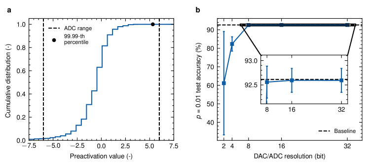
Figure S1: ADC/DAC range and resolution. (a) Experiment to determine an appropriate ADC range. The plot shows the cumulative distribution of the pre-activation values, that is, the values before applying the activation function during inference, for 1024 sequences of syndromes selected randomly in the dataset generated at a physical fault rate of 0.01. The black dot denotes the 99.99-th percentile of this distribution. The ADC range is selected to be the smallest integer above, which is $6$ in this case. (b) Impact of the ADC/DAC resolution on the neural decoder’s test accuracy at a physical fault rate of 0.01. The test accuracy is obtained without including programming variability or defective devices, in order to assess the impact of resolution alone. At an 8-bit resolution, that is, 256 discretization steps between the boundary values $-6$ and $6$ determined in (a), the accuracy gets sufficiently close to the baseline accuracy (without discretization, or equivalent to an infinite resolution). The error bars are obtained from 100 inference runs averaged over 10 training runs.

Supplementary Information Note 3: Experiments on TiO_x memristive devices

The TiO_x memristive devices are characterized by a Keysight Technologies B1500A semiconductor device parameter analyzer that has a 200 M samples/second waveform generator/fast measurement unit (WGFMU) on a Lake Shore CPX-VF probe station at room temperature. For all measurements, the bottom electrodes are grounded and the signals are applied to the top electrodes.

Conductance state programming

Memristive devices’ resistances are programmed using a closed-loop read–write–verify algorithm [47, 30]. This algorithm allows the programming of a resistive memory device to a target resistance by applying successive read and write pulses. Initially, the device resistance is read using a read pulse (0.2 V amplitude per $1\text{\,}\mathrm{\SIUnitSymbolMicro s}$ pulse width). If this measured resistance is larger than the target within a 1% tolerance, a positive write pulse is applied ($\approx$1 V amplitude per 200 ns pulse width); if it is lower, a negative pulse is applied. A read pulse is then applied to check the new resistance state, which starts a new loop. The pulse amplitude is increased after each consecutive pulses of the same polarity by a constant step in order to converge to the target resistance. Using this read–write–verify algorithm for various target levels of resistance, we can perform multilevel programming as in Fig. 4(a).

Programming variability characterization

The programming variability model is based on experimental measurement on TiO_x-based memristive devices. As shown in Fig. 5(a), multilevel programming is performed from the high-conductance state to the low-conductance state and successively from the low-conductance state to the high-conductance state 10 times to assess the cycle-to-cycle programming variability. For each state and at each multilevel programming pass, the conductance is read 20 times and the mean value is kept. This process is repeated for 10 memristive devices to include device-to-device variability in the programming error model. The histogram of the mean programmed values for a conductance state is fitted by a Gaussian distribution and its standard deviation is extracted (depicted in Fig. 5(b)).

Supplementary Note 4: Computational Methods

Implementation of training and inference

The training of the RNN always starts with a classical deep learning [74] optimization process (referred as FP training), using PyTorch [75] with no consideration for hardware non-idealities. The meta-parameters used during this step are described in Table S1. In the case of HWA and DS retraining, the RNN parameters (weights and biases) are loaded from the previous FP training, and 10 additional epochs are run to adapt the model to newly introduced hardware constraints. Every other meta-parameter remains unchanged during the retraining.

Meta-parameters	Values
Input size	4 $\times$ 4 rounds
Hidden layer size	16
Activation function	ReLU
Batch size	32
Loss	Cross entropy
Optimizer	Adam [76]
Learning rate	0.001

Table S1: Model and training meta-parameters.

The RNN retraining and inference simulations are performed using the IBM Analog Hardware Acceleration Kit [77]. This toolkit is used to emulate the computations executed on a crossbar array of memristive devices. In our case, we extend recurrent network modules of the PyTorch library using the toolkit to simulate the behaviour of a memristive RNN. We extend the original toolkit to consider the specific TiO_x resistive memory devices used in our work. The non-idealities we discuss in the hardware characterization section are implemented in the simulator. For instance, the statistical programming variability is calibrated on our TiO_x devices.

Hardware-aware training methods

For hardware-aware training, the main manuscript focuses on introducing dropconnect during the retraining of the memristive neural decoder to mitigate the effect of defective devices in the chip. Having said that, there are other training methods that could improve performance. One such method would be to inject noise on weights during training to account for the programming variability of TiO₂ devices. It has been shown that setting the training weight variability approximately equal to the inference weight variability [35] is optimal. From the programming variability model obtained in the manuscript, this represents an injection of a $0.8\%$ Gaussian noise during training. Also, input/output discretization during training could mitigate the impact of ADC/DAC-limited resolution during inference. An intuitive choice is to set the training discretization at the same resolution as ADC/DAC, that is, 8-bit resolution in our case.

We perform hardware-aware training of memristive neural decoders with all possible combinations of the three techniques (dropconnect, noise injection, and input/output discretization). The results are displayed in Supplementary Table S2. The conclusion is that only dropconnect has a critical effect on the performance of the decoding. We attribute this to the fact that TiO₂ resistive memory devices exhibit a low programming variability (in comparison to PCM devices reported in [35]); therefore, injecting noise during training does not significantly improve accuracy. Also, an ADC/DAC 8-bit resolution is sufficient for maintaining good accuracy, as explained in Supplementary Information Note 1. Thus, input/output discretization during training does not allow a greater accuracy.

Another training method reported to improve test accuracy with IMC is weight clipping [35]. It allows a certain degree of control over the weight distribution to make the programming of weights to hardware easier. It is performed by clipping the weights of a layer, after each update pass, within the range $[-\alpha\sigma;\alpha\sigma]$, where $\alpha$ is referred to as the clip scale, and $\sigma$ is the standard deviation of the weight distribution of that layer. We tested different clip scales to find its optimal value, as shown in Supplementary Fig. S2. The conclusion is that weight clipping during training does not improve the test accuracy. The accuracy reached without clipping is very similar. We attribute this to the fact that our programming variability is low; thus, the conductances can be reliably programmed even if their corresponding weights are close to one another.

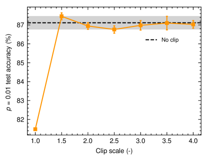
Figure S2: Impact of weight clipping during training. During training, the weights are clipped within the range $[-\alpha\sigma;\alpha\sigma]$, where $\alpha$ is the clip scale. It can be seen that different clip scales do not seem to improve the test accuracy compared to a lack of clipping during training.

Drop connections	Noise injection	IO discretization	$p=10^{-2}$ test accuracy (%)
No	No	No	$(76.6248\pm 0.6578)$
No	No	Yes	$(77.0062\pm 0.5999)$
No	Yes	No	$(76.7334\pm 0.6219)$
No	Yes	Yes	$(77.0741\pm 0.6157)$
Yes	No	No	$(86.8568\pm 0.3344)$
Yes	No	Yes	$(86.8251\pm 0.1857)$
Yes	Yes	No	$(86.8379\pm 0.2924)$
Yes	Yes	Yes	$(86.7605\pm 0.2041)$

Table S2: Hardware-aware supplementary training methods. Test accuracy at a physical fault rate of $10^{-2}$ for memristive neural decoders trained with different combinations of hardware-aware techniques.

References

- Shor [1994] P. W. Shor, Algorithms for quantum computation: discrete logarithms and factoring, in Proceedings 35th annual symposium on foundations of computer science (Ieee, 1994) pp. 124–134.
- Gidney and Ekerå [2021] C. Gidney and M. Ekerå, How to factor 2048 bit rsa integers in 8 hours using 20 million noisy qubits, Quantum 5, 433 (2021).
- Preskill [1998] J. Preskill, Reliable quantum computers, Proceedings of the Royal Society of London. Series A: Mathematical, Physical and Engineering Sciences 454, 385 (1998).
- Roffe [2019] J. Roffe, Quantum error correction: an introductory guide, Contemporary Physics 60, 226 (2019).
- Battistel et al. [2023] F. Battistel, C. Chamberland, K. Johar, R. W. Overwater, F. Sebastiano, L. Skoric, Y. Ueno, and M. Usman, Real-time decoding for fault-tolerant quantum computing: Progress, challenges and outlook, arXiv preprint arXiv:2303.00054 (2023).
- Charbon et al. [2016] E. Charbon, F. Sebastiano, A. Vladimirescu, H. Homulle, S. Visser, L. Song, and R. M. Incandela, Cryo-cmos for quantum computing, in 2016 IEEE International Electron Devices Meeting (IEDM) (IEEE, 2016) pp. 13–5.
- Xue et al. [2021] X. Xue, B. Patra, J. P. van Dijk, N. Samkharadze, S. Subramanian, A. Corna, B. Paquelet Wuetz, C. Jeon, F. Sheikh, E. Juarez-Hernandez, et al., Cmos-based cryogenic control of silicon quantum circuits, Nature 593, 205 (2021).
- Underwood et al. [2023] D. L. Underwood, J. A. Glick, K. Inoue, D. J. Frank, J. Timmerwilke, E. Pritchett, S. Chakraborty, K. Tien, M. Yeck, J. F. Bulzacchelli, et al., Using cryogenic cmos control electronics to enable a two-qubit cross-resonance gate, arXiv preprint arXiv:2302.11538 (2023).
- McDermott et al. [2018] R. McDermott, M. Vavilov, B. Plourde, F. Wilhelm, P. Liebermann, O. Mukhanov, and T. Ohki, Quantum–classical interface based on single flux quantum digital logic, Quantum science and technology 3, 024004 (2018).
- Razmkhah et al. [2022] S. Razmkhah, A. Bozbey, and P. Febvre, Superconductor modulation circuits for qubit control at microwave frequencies, arXiv preprint arXiv:2211.06667 (2022).
- Yohannes et al. [2023] D. Yohannes, M. Renzullo, J. Vivalda, A. Jacobs, M. Yu, J. Walter, A. Kirichenko, I. Vernik, and O. Mukhanov, High density fabrication process for single flux quantum circuits, Applied Physics Letters 122 (2023).
- Czischek et al. [2021] S. Czischek, V. Yon, M.-A. Genest, M.-A. Roux, S. Rochette, J. C. Lemyre, M. Moras, M. Pioro-Ladrière, D. Drouin, Y. Beilliard, et al., Miniaturizing neural networks for charge state autotuning in quantum dots, Machine Learning: Science and Technology 3, 015001 (2021).
- Holmes et al. [2020] A. Holmes, M. R. Jokar, G. Pasandi, Y. Ding, M. Pedram, and F. T. Chong, Nisq+: Boosting quantum computing power by approximating quantum error correction, in 2020 ACM/IEEE 47th Annual International Symposium on Computer Architecture (ISCA) (IEEE, 2020) pp. 556–569.
- Ueno et al. [2021] Y. Ueno, M. Kondo, M. Tanaka, Y. Suzuki, and Y. Tabuchi, Qecool: On-line quantum error correction with a superconducting decoder for surface code, in 2021 58th ACM/IEEE Design Automation Conference (DAC) (IEEE, 2021) pp. 451–456.
- Ueno et al. [2022a] Y. Ueno, M. Kondo, M. Tanaka, Y. Suzuki, and Y. Tabuchi, Qulatis: A quantum error correction methodology toward lattice surgery, in 2022 IEEE International Symposium on High-Performance Computer Architecture (HPCA) (IEEE, 2022) pp. 274–287.
- Ueno et al. [2022b] Y. Ueno, M. Kondo, M. Tanaka, Y. Suzuki, and Y. Tabuchi, Neo-qec: Neural network enhanced online superconducting decoder for surface codes, arXiv preprint arXiv:2208.05758 (2022b).
- Delfosse and Nickerson [2021] N. Delfosse and N. H. Nickerson, Almost-linear time decoding algorithm for topological codes, Quantum 5, 595 (2021).
- Wu et al. [2022] Y. Wu, N. Liyanage, and L. Zhong, An interpretation of union-find decoder on weighted graphs, arXiv preprint arXiv:2211.03288 (2022).
- Chamberland et al. [2020] C. Chamberland, A. Kubica, T. J. Yoder, and G. Zhu, Triangular color codes on trivalent graphs with flag qubits, New Journal of Physics 22, 023019 (2020).
- Chamberland and Ronagh [2018] C. Chamberland and P. Ronagh, Deep neural decoders for near term fault-tolerant experiments, Quantum Science and Technology 3, 044002 (2018).
- Verma et al. [2019] N. Verma, H. Jia, H. Valavi, Y. Tang, M. Ozatay, L.-Y. Chen, B. Zhang, and P. Deaville, In-memory computing: Advances and prospects, IEEE Solid-State Circuits Magazine 11, 43 (2019).
- El Mesoudy et al. [2022] A. El Mesoudy, G. Lamri, R. Dawant, J. Arias-Zapata, P. Gliech, Y. Beilliard, S. Ecoffey, A. Ruediger, F. Alibart, and D. Drouin, Fully cmos-compatible passive tio2-based memristor crossbars for in-memory computing, Microelectronic Engineering 255, 111706 (2022).
- Berggren et al. [2020] K. Berggren, Q. Xia, K. K. Likharev, D. B. Strukov, H. Jiang, T. Mikolajick, D. Querlioz, M. Salinga, J. R. Erickson, S. Pi, et al., Roadmap on emerging hardware and technology for machine learning, Nanotechnology 32, 012002 (2020).
- Chua [1971] L. Chua, Memristor-the missing circuit element, IEEE Transactions on Circuit Theory 18, 507 (1971).
- Strukov et al. [2008] D. B. Strukov, G. S. Snider, D. R. Stewart, and R. S. Williams, The missing memristor found, Nature 453, 80 (2008).
- Chua [2011] L. Chua, Resistance switching memories are memristors, Applied Physics A 102, 765 (2011).
- Song et al. [2023] M.-K. Song, J.-H. Kang, X. Zhang, W. Ji, A. Ascoli, I. Messaris, A. S. Demirkol, B. Dong, S. Aggarwal, W. Wan, S.-M. Hong, S. G. Cardwell, I. Boybat, J. sun Seo, J.-S. Lee, M. Lanza, H. Yeon, M. Onen, J. Li, B. Yildiz, J. A. del Alamo, S. Kim, S. Choi, G. Milano, C. Ricciardi, L. Alff, Y. Chai, Z. Wang, H. Bhaskaran, M. C. Hersam, D. Strukov, H.-S. P. Wong, I. Valov, B. Gao, H. Wu, R. Tetzlaff, A. Sebastian, W. Lu, L. Chua, J. J. Yang, and J. Kim, Recent advances and future prospects for memristive materials, devices, and systems, ACS Nano 17, 11994 (2023).
- Amirsoleimani et al. [2020] A. Amirsoleimani, F. Alibart, V. Yon, J. Xu, M. R. Pazhouhandeh, S. Ecoffey, Y. Beilliard, R. Genov, and D. Drouin, In‐Memory Vector‐Matrix Multiplication in Monolithic Complementary Metal–Oxide–Semiconductor‐Memristor Integrated Circuits: Design Choices, Challenges, and Perspectives, Advanced Intelligent Systems 2, 2000115 (2020).
- Beilliard et al. [2020] Y. Beilliard, F. Paquette, F. Brousseau, S. Ecoffey, F. Alibart, and D. Drouin, Conductive filament evolution dynamics revealed by cryogenic (1.5 k) multilevel switching of CMOS-compatible al2o3/tio2 resistive memories, Nanotechnology 31, 445205 (2020).
- Mouny et al. [2023] P.-A. Mouny, Y. Beilliard, S. Graveline, M.-A. Roux, A. E. Mesoudy, R. Dawant, P. Gliech, S. Ecoffey, F. Alibart, M. Pioro-Ladrière, and D. Drouin, Memristor-based cryogenic programmable dc sources for scalable in situ quantum-dot control, IEEE Transactions on Electron Devices 70, 1989 (2023).
- Wang et al. [2020] P. Wang, X. Peng, W. Chakraborty, A. I. Khan, S. Datta, and S. Yu, Cryogenic Benchmarks of Embedded Memory Technologies for Recurrent Neural Network based Quantum Error Correction, in 2020 IEEE International Electron Devices Meeting (IEDM) (2020) pp. 38.5.1–38.5.4.
- Ichikawa et al. [2022a] Y. Ichikawa, A. Goda, C. Matsui, and K. Takeuchi, Non-volatile Memory Application to Quantum Error Correction with Non-uniformly Quantized CiM, in 2022 IEEE International Memory Workshop (IMW) (2022) pp. 1–4.
- Ichikawa et al. [2022b] Y. Ichikawa, A. Goda, C. Matsui, and K. Takeuchi, Non-volatile memory application to quantum error correction with non-uniformly quantized cim, in 2022 IEEE International Memory Workshop (IMW) (IEEE, 2022) pp. 1–4.
- Baireuther et al. [2019] P. Baireuther, M. D. Caio, B. Criger, C. W. J. Beenakker, and T. E. O’Brien, Neural network decoder for topological color codes with circuit level noise, New Journal of Physics 21, 013003 (2019).
- Joshi et al. [2020] V. Joshi, M. Le Gallo, S. Haefeli, I. Boybat, S. R. Nandakumar, C. Piveteau, M. Dazzi, B. Rajendran, A. Sebastian, and E. Eleftheriou, Accurate deep neural network inference using computational phase-change memory, Nature Communications 11, 2473 (2020).
- Bombin and Martin-Delgado [2007] H. Bombin and M. A. Martin-Delgado, Optimal resources for topological two-dimensional stabilizer codes: Comparative study, Phys. Rev. A 76, 012305 (2007).
- Horsman et al. [2012] C. Horsman, A. G. Fowler, S. Devitt, and R. Van Meter, Surface code quantum computing by lattice surgery, New Journal of Physics 14, 123011 (2012).
- Tomita and Svore [2014] Y. Tomita and K. M. Svore, Low-distance surface codes under realistic quantum noise, Physical Review A 90, 062320 (2014).
- Baireuther et al. [2018] P. Baireuther, T. E. O’Brien, B. Tarasinski, and C. W. J. Beenakker, Machine-learning-assisted correction of correlated qubit errors in a topological code, Quantum 2, 48 (2018).
- Litinski [2019] D. Litinski, A game of surface codes: Large-scale quantum computing with lattice surgery, Quantum 3, 128 (2019).
- Varsamopoulos et al. [2020a] S. Varsamopoulos, K. Bertels, and C. G. Almudever, Decoding surface code with a distributed neural network–based decoder, Quantum Machine Intelligence 2, 3 (2020a).
- Delfosse [2020a] N. Delfosse, Hierarchical decoding to reduce hardware requirements for quantum computing, arXiv preprint arXiv:2001.11427 (2020a).
- Chamberland and Beverland [2018] C. Chamberland and M. E. Beverland, Flag fault-tolerant error correction with arbitrary distance codes, Quantum 2, 53 (2018).
- Gokmen et al. [2018] T. Gokmen, M. J. Rasch, and W. Haensch, Training LSTM Networks With Resistive Cross-Point Devices, Frontiers in Neuroscience 12 (2018).
- Hu et al. [2018] M. Hu, C. E. Graves, C. Li, Y. Li, N. Ge, E. Montgomery, N. Davila, H. Jiang, R. S. Williams, J. J. Yang, Q. Xia, and J. P. Strachan, Memristor-based analog computation and neural network classification with a dot product engine, Advanced Materials 30, 10.1002/adma.201705914 (2018).
- Milo et al. [2020] V. Milo, G. Malavena, C. Monzio Compagnoni, and D. Ielmini, Memristive and CMOS Devices for Neuromorphic Computing, Materials 13, 166 (2020).
- Alibart et al. [2012] F. Alibart, L. Gao, B. D. Hoskins, and D. B. Strukov, High precision tuning of state for memristive devices by adaptable variation-tolerant algorithm, Nanotechnology 23, 075201 (2012).
- Ielmini and Wong [2018] D. Ielmini and H.-S. P. Wong, In-memory computing with resistive switching devices, Nature Electronics 1, 333 (2018).
- Zhang et al. [2020] Y. Zhang, P. Huang, B. Gao, J. Kang, and H. Wu, Oxide-based filamentary RRAM for deep learning, Journal of Physics D: Applied Physics 54, 083002 (2020).
- Adam et al. [2018] G. C. Adam, A. Khiat, and T. Prodromakis, Challenges hindering memristive neuromorphic hardware from going mainstream, Nature Communications 9, 10.1038/s41467-018-07565-4 (2018).
- Wang et al. [2019] C. Wang, D. Feng, W. Tong, J. Liu, Z. Li, J. Chang, Y. Zhang, B. Wu, J. Xu, W. Zhao, Y. Li, and R. Ren, Cross-point resistive memory, ACM Transactions on Design Automation of Electronic Systems 24, 1 (2019).
- Yon et al. [2022] V. Yon, A. Amirsoleimani, F. Alibart, R. G. Melko, D. Drouin, and Y. Beilliard, Exploiting non-idealities of resistive switching memories for efficient machine learning, Frontiers in Electronics 3, 10.3389/felec.2022.825077 (2022).
- Chen et al. [2015] C.-Y. Chen, H.-C. Shih, C.-W. Wu, C.-H. Lin, P.-F. Chiu, S.-S. Sheu, and F. T. Chen, Rram defect modeling and failure analysis based on march test and a novel squeeze-search scheme, IEEE Transactions on Computers 64, 180 (2015).
- Kim et al. [2021] H. Kim, M. R. Mahmoodi, H. Nili, and D. B. Strukov, 4k-memristor analog-grade passive crossbar circuit, Nature Communications 12, 10.1038/s41467-021-25455-0 (2021).
- Jang et al. [2022] J. Jang, S. Gi, I. Yeo, S. Choi, S. Jang, S. Ham, B. Lee, and G. Wang, A learning-rate modulable and reliable TiOx memristor array for robust, fast, and accurate neuromorphic computing, Advanced Science 9, 2201117 (2022).
- Yeon et al. [2020] H. Yeon, P. Lin, C. Choi, S. H. Tan, Y. Park, D. Lee, J. Lee, F. Xu, B. Gao, H. Wu, H. Qian, Y. Nie, S. Kim, and J. Kim, Alloying conducting channels for reliable neuromorphic computing, Nature Nanotechnology 15, 574 (2020).
- Hu et al. [2016] M. Hu, J. P. Strachan, Z. Li, E. M. Grafals, N. Davila, C. Graves, S. Lam, N. Ge, J. J. Yang, and R. S. Williams, Dot-product engine for neuromorphic computing: Programming 1t1m crossbar to accelerate matrix-vector multiplication, in 2016 53nd ACM/EDAC/IEEE Design Automation Conference (DAC) (2016) pp. 1–6.
- Blundell et al. [2015] C. Blundell, J. Cornebise, K. Kavukcuoglu, and D. Wierstra, Weight uncertainty in neural networks, in Proceedings of the 32nd International Conference on International Conference on Machine Learning - Volume 37, ICML’15 (JMLR.org, 2015) p. 1613–1622.
- Gulcehre et al. [2016] C. Gulcehre, M. Moczulski, M. Denil, and Y. Bengio, Noisy activation functions, in Proceedings of the 33rd International Conference on International Conference on Machine Learning - Volume 48, ICML’16 (JMLR.org, 2016) p. 3059–3068.
- Wan et al. [2013] L. Wan, M. Zeiler, S. Zhang, Y. Le Cun, and R. Fergus, Regularization of neural networks using dropconnect, in Proceedings of the 30th International Conference on Machine Learning, Proceedings of Machine Learning Research, Vol. 28, edited by S. Dasgupta and D. McAllester (PMLR, Atlanta, Georgia, USA, 2013) pp. 1058–1066.
- Hinton et al. [2012] G. E. Hinton, N. Srivastava, A. Krizhevsky, I. Sutskever, and R. R. Salakhutdinov, Improving neural networks by preventing co-adaptation of feature detectors, Preprint at https://arxiv.org/abs/1207.0580 (2012).
- Chen et al. [2017] L. Chen, J. Li, Y. Chen, Q. Deng, J. Shen, X. Liang, and L. Jiang, Accelerator-friendly neural-network training: Learning variations and defects in rram crossbar, in Design, Automation & Test in Europe Conference & Exhibition (DATE), 2017 (2017) pp. 19–24.
- van de Goor and Zorian [1993] A. van de Goor and Y. Zorian, Effective march algorithms for testing single-order addressed memories, in 1993 European Conference on Design Automation with the European Event in ASIC Design (1993) pp. 499–505.
- Chen and Li [2015] Y.-X. Chen and J.-F. Li, Fault modeling and testing of 1t1r memristor memories, in 2015 IEEE 33rd VLSI Test Symposium (VTS) (2015) pp. 1–6.
- Surekcigil Pesch et al. [2022] I. Surekcigil Pesch, E. Bestelink, O. de Sagazan, A. Mehonic, and R. A. Sporea, Multimodal transistors as ReLU activation functions in physical neural network classifiers, Scientific Reports 12, 10.1038/s41598-021-04614-9 (2022).
- Liu et al. [2014] B. Liu, H. Li, Y. Chen, X. Li, T. Huang, Q. Wu, and M. Barnell, Reduction and ir-drop compensations techniques for reliable neuromorphic computing systems, in 2014 IEEE/ACM International Conference on Computer-Aided Design (ICCAD) (2014) pp. 63–70.
- Liu et al. [2015] B. Liu, H. Li, Y. Chen, X. Li, Q. Wu, and T. Huang, Vortex: Variation-aware training for memristor x-bar, in 2015 52nd ACM/EDAC/IEEE Design Automation Conference (DAC) (2015) pp. 1–6.
- Delfosse [2020b] N. Delfosse, Hierarchical decoding to reduce hardware requirements for quantum computing, Preprint at http://arxiv.org/abs/2001.11427 (2020b).
- Meinerz et al. [2022] K. Meinerz, C.-Y. Park, and S. Trebst, Scalable neural decoder for topological surface codes, Phys. Rev. Lett. 128, 080505 (2022).
- Varsamopoulos et al. [2020b] S. Varsamopoulos, K. Bertels, and C. G. Almudever, Comparing Neural Network Based Decoders for the Surface Code, IEEE Transactions on Computers 69, 300 (2020b).
- Chamberland et al. [2022] C. Chamberland, L. Goncalves, P. Sivarajah, E. Peterson, and S. Grimberg, Techniques for combining fast local decoders with global decoders under circuit-level noise, Preprint at https://arxiv.org/abs/2208.01178 (2022).
- Gidney [2021] C. Gidney, Stim: a fast stabilizer circuit simulator, Quantum 5, 497 (2021).
- Higgott [2021] O. Higgott, Pymatching: A python package for decoding quantum codes with minimum-weight perfect matching (2021), arXiv:2105.13082 [quant-ph] .
- LeCun et al. [2015] Y. LeCun, Y. Bengio, and G. Hinton, Deep learning, nature 521, 436 (2015).
- Paszke et al. [2019] A. Paszke, S. Gross, F. Massa, A. Lerer, J. Bradbury, G. Chanan, T. Killeen, Z. Lin, N. Gimelshein, L. Antiga, A. Desmaison, A. Kopf, E. Yang, Z. DeVito, M. Raison, A. Tejani, S. Chilamkurthy, B. Steiner, L. Fang, J. Bai, and S. Chintala, PyTorch: An Imperative Style, High-Performance Deep Learning Library, in Advances in Neural Information Processing Systems 32, edited by H. Wallach, H. Larochelle, A. Beygelzimer, F. d’Alché Buc, E. Fox, and R. Garnett (Curran Associates, Inc., 2019) pp. 8024–8035.
- Kingma and Ba [2017] D. P. Kingma and J. Ba, Adam: A method for stochastic optimization (2017), arXiv:1412.6980 [cs.LG] .
- Rasch et al. [2021] M. J. Rasch, D. Moreda, T. Gokmen, M. Le Gallo, F. Carta, C. Goldberg, K. El Maghraoui, A. Sebastian, and V. Narayanan, A flexible and fast pytorch toolkit for simulating training and inference on analog crossbar arrays, in 2021 IEEE 3rd International Conference on Artificial Intelligence Circuits and Systems (AICAS) (2021) pp. 1–4.