[a]Jacopo Ghiglieri

Hard parton dispersion in the quark-gluon plasma, non-perturbatively

   Guy D. Moore    Philipp Schicho    Niels Schlusser    Eamonn Weitz
Abstract

The in-medium dispersion of hard partons, encoded in their so-called asymptotic mass, receives large non-perturbative contributions from classical gluons, i.e. soft gluons with large occupation numbers. Here, we discuss how the analytical properties of thermal amplitudes allow for a non-perturbative determination of the infrared classical contribution through lattice determinations in the dimensionally-reduced effective theory of hot QCD, EQCD. We show how these lattice determinations need to be complemented by perturbative two-loop matching calculations between EQCD and QCD, so that the unphysical (classical) ultraviolet behavior of EQCD is replaced by its proper quantum QCD counterpart. We show how lattice and perturbative EQCD are in good agreement in the UV and present an outlook on the two-loop quantum QCD contribution.

1 Introduction

Jets are a key hard probe in the theoretical and experimental investigation of the Quark-Gluon Plasma (QGP), an exotic state of strongly interacting matter. Their study provides important experimental sources of evidence about the nature of Quantum Chromodynamics (QCD) under extreme conditions – see [1, 2, 3] for recent reviews.

Here, we focus on jets created by light quarks ($u,d,s$) or gluons. While massless in vacuum, high-energy particles with momentum $\bm{p}$ follow the dispersion relation of massive particles when traversing a QGP of temperature $T$, $\omega_{\bm{p}}^{2}=\bm{p}^{2}+m^{2}_{\bm{p}}$, as found independently by Klimov [4] and Weldon [5, 6]. This effective mass arises through forward scattering with the medium. At very large momentum, it is called the asymptotic mass and it is an important ingredient in the determination of medium-induced radiation rates and transport coefficients, see [7] for a review.

To one-loop order, these masses are given by the gauge and the fermion condensates $Z_{\rm g}$ and $Z_{\rm f}$:

$$m_{\infty,{\rm q}}^{2}=g^{2}C_{\mbox{\tiny\rm{F}}}\Bigl{(}Z_{\rm g}+Z_{\rm f}\Bigr{)}\,,\qquad m_{\infty,{\rm g}}^{2}=g^{2}C_{\mbox{\tiny\rm{A}}}Z_{\rm g}+2g^{2}T_{\mbox{\tiny\rm{F}}}N_{\mbox{\scriptsize f}}Z_{\rm f}\,,$$ (1)

where $m_{\infty,{\rm q}}^{2}$ for quarks and $m_{\infty,{\rm g}}^{2}$ for gluons. Here $C_{\mbox{\tiny\rm{F}}}=4/3$ and $C_{\mbox{\tiny\rm{A}}}=3$ are the quark and gluon quadratic Casimir, $N_{\mbox{\scriptsize f}}$ is the number of light quark species, and $T_{\mbox{\tiny\rm{F}}}=1/2$ is the trace normalization of the fundamental representation. The condensates $Z_{\rm g}$ and $Z_{\rm f}$ are non-local and have a gauge-invariant definition in terms of correlators [8, 9]

$$Z_{\rm f}\equiv\frac{1}{6}\Big{\langle}\overline{\psi}\frac{v_{\mu}\gamma^{\mu}}{v\cdot D}\psi\Big{\rangle}\;,\qquad Z_{\rm g}\equiv-\frac{1}{8}\Big{\langle}v_{\alpha}F^{\alpha\mu}\frac{1}{(v\cdot D)^{2}}v_{\nu}F^{\nu}_{\;\;\mu}\Big{\rangle}\;,$$ (2)

where $v^{\mu}=(1,0,0,1)$ is the four-velocity of the hard particle and $\langle\dots\rangle$ denotes a thermal expectation value. Our conventions are as in [10].

Eq. (1) arises from integrating out the energy scale of the jet $p\sim E\gg T$, truncating at first order in $T/E$ and determining the matching coefficients at $\mathcal{O}(g^{0})$. If $E\gtrsim T$, higher orders in the $T/E$ expansion can become relevant beyond one-loop order and spoil the factorization into fermionic and bosonic condensates of (1). In coordinate space, the inverse of a covariant derivative is an integral over separation of a Wilson line $U$. $Z_{\rm g}$ is then an integral over $x^{+}\equiv(x^{0}+x^{z})/2$ of a correlator of two Lorentz-force insertions

$$Z_{\rm g}\equiv-\frac{1}{4}\int_{0}^{\infty}\!{\rm d}x^{+}x^{+}\,\mathrm{Tr}\,\Bigl{\langle}U(-\infty;x^{+})v_{\mu}F^{\mu\nu}(x^{+})\,U(x^{+};0)\,v_{\rho}F^{\rho}_{\,\nu}(0)U(0;-\infty)\Bigr{\rangle}\;,$$ (3)

with $F_{\mu\nu}=F_{\mu\nu}^{a}T^{a}$. $T^{a}$ is in the fundamental representation. So are the Wilson lines, which source path-ordered gluons along the $x^{+}$ light-cone direction. At leading order (LO), one easily finds [4, 5, 6]

$$Z_{\rm g}\big{|}^{\mathrm{LO}}=\frac{1}{\pi^{2}}\int_{0}^{\infty}{\rm d}q\,q\,n_{\mbox{\scriptsize B}}(q)=\frac{T^{2}}{6},\qquad Z_{\rm f}\big{|}^{\mathrm{LO}}=\frac{1}{\pi^{2}}\int_{0}^{\infty}{\rm d}q\,q\,n_{\mbox{\scriptsize F}}(q)=\frac{T^{2}}{12}.$$ (4)

The first correction to this affects $Z_{\rm g}$ only and does not come from extra loops but from a more careful evaluation of the infrared (IR). As $n_{\mbox{\scriptsize B}}(q\ll T)\approx\frac{T}{q}\gg 1$, soft ($q\sim gT$) gluons are classical and their contribution represents an $\mathcal{O}(g)$ correction, which can be evaluated by properly accounting for the collective effects that arise at that scale. This was done in [9], yielding the next-to-leading order (NLO) viz. $Z_{\rm g}\big{|}^{\mathrm{NLO}}=-Tm_{\mbox{\tiny\rm{D}}}/(2\pi)$, where $m_{\mbox{\tiny\rm{D}}}=gT\sqrt{1+N_{\mbox{\scriptsize f}}/6}$ is the Debye mass. This remarkable result was obtained, following [11], by exploiting the analytical properties of thermal amplitudes at space- and light-like separations to map the classical contribution to Eq. (3) to its counterpart $Z_{\rm g}^{{\mbox{\tiny\rm{3d}}}}$ in Electrostatic QCD (EQCD). EQCD [12, 13, 14, 15, 16] is a dimensionally-reduced (3D) Effective Field Theory (EFT) that describes the Matsubara zero-modes of the gauge fields, integrating out all non-zero quark and gluon modes.

This mapping is remarkable: as $Z_{\rm g}^{{\mbox{\tiny\rm{3d}}}}$ can be determined non-perturbatively in lattice EQCD, this then gives an all-order determination of the classical contribution to $Z_{\rm g}$. In general, the classical soft and ultrasoft ($q\sim g^{2}T$) modes are responsible for the slow convergence — or outright breakdown in the latter case [17] — of thermal perturbation theory. Hence, the availability of a non-perturbative determination circumvents this issue. In this contribution, we then discuss the necessary steps in lattice and continuum EQCD, as well as in perturbative thermal QCD, to reach this goal. This is based on [18, 10, 19], to which we refer for further details. A similar program has already been carried out in [20, 21] for the transverse scattering kernel.

2 Lattice determination

The continuum EQCD action reads

$$S_{{\mbox{\tiny\rm{EQCD}}},c}=\int_{{\bf x}}\bigg{\{}\frac{1}{2}\mathrm{Tr}\,F_{ij}F_{ij}+\mathrm{Tr}\,[D_{i},\Phi][D_{i},\Phi]+m_{\mbox{\tiny\rm{D}}}^{2}\mathrm{Tr}\,\Phi^{2}+\lambda_{\mbox{\tiny\rm{E}}}(\mathrm{Tr}\,\Phi^{2})^{2}\bigg{\}}\,.$$ (5)

Under dimensional reduction $A^{0}$ becomes an adjoint scalar, $A^{0}\to-i\Phi$, $\lambda_{\mbox{\tiny\rm{E}}}\sim g^{4}T$ and $g_{{\mbox{\tiny\rm{3d}}}}^{2}\approx g^{2}T$ is the dimensionful gauge coupling [16], making EQCD super-renormalizeable. The EQCD contribution to Eq. (3) is then

$$Z_{\rm g}^{{\mbox{\tiny\rm{3d}}}}=\frac{T}{2}\int_{0}^{\infty}\!\!{\rm d}L\,L\,\langle FF\rangle,\text{ where }\langle FF\rangle\equiv\bigl{(}\langle EE\rangle-\langle BB\rangle-i\langle EB\rangle\bigr{)}\;,\text{ and }E=D_{x}\Phi,\;\;B=F_{xz}.$$ (6)

$\langle EE\rangle\equiv\frac{1}{2}\bigl{\langle}(D_{x}\Phi(L))^{a}\,\tilde{U}^{ab}_{\mbox{\tiny\rm{A}}}(L,0)\,(D_{x}\Phi(0))^{b}\bigr{\rangle}$ and similarly for $\langle BB\rangle$ and $i\langle EB\rangle$. Under dimensional reduction $x^{+}\to L$, which, together with the rotation of $A^{0}$ in the complex plane, turns the adjoint Wilson line into a non-unitary 3D equivalent $\tilde{U}^{ab}_{\mbox{\tiny\rm{A}}}(L,0)$, see [18].

Lattice EQCD provides us with continuum-extrapolated values for the three correlators $\langle EE\rangle$, $\langle BB\rangle$ and $i\langle EB\rangle$ at discrete values of the separation $L$ in the range $0.25<g_{{\mbox{\tiny\rm{3d}}}}^{2}L<3$ at four different temperatures — see [18, 10] for details on discretization, renormalization and continuum extrapolation. Eq. (6) requires an integral over all values of $L$. The IR range at large $g_{{\mbox{\tiny\rm{3d}}}}^{2}L\gg 1$ can be addressed by a fitting ansatz based on the expected exponential falloff from electrostatic and magnetostatic screening. At short distances, on the other hand, not only are we limited by lattice spacing and increasing discretization effects, but we need to address the fact that the UV of EQCD, as for any IR EFT, differs from the UV of QCD, as we now discuss.

3 Ultraviolet matching

In the deep UV ($m_{\mbox{\tiny\rm{D}}}L\ll 1$), we expect perturbative EQCD (pEQCD) to be applicable; furthermore, this is where super-renormalizability comes in handy, since it dictates that

$$\langle FF\rangle_{m_{\mbox{\tiny\rm{D}}}L\ll 1}=\frac{c_{0}}{L^{3}}+\frac{c_{2}g_{{\mbox{\tiny\rm{3d}}}}^{2}}{L^{2}}+\frac{c_{4}g_{{\mbox{\tiny\rm{3d}}}}^{4}}{L}+\ldots\,,$$ (7)

with constants $c_{i}$ arising from short-distance pEQCD. Only the first two terms will be divergent when plugged in Eq. (6). $c_{0}/L^{3}$ gives rise to a power-law divergence: indeed, the classical contribution to Eq. (4), obtained from $n_{\mbox{\scriptsize B}}(q)\to\frac{T}{q}$, is linearly UV divergent. These two divergences are opposite and, if evaluated in the same scheme, cancel: the UV of EQCD, where $m_{\mbox{\tiny\rm{D}}}$ and $\lambda_{\mbox{\tiny\rm{E}}}$ are negligible, must agree with the IR of bare 4D QCD. As the bare 4D QCD IR is included in Eq. (4), we can simply subtract $c_{0}/L^{3}$ $\forall L$ on the EQCD side. A simple calculation finds $c_{0}=2/\pi$.

At NLO in pEQCD, $c_{2}g_{{\mbox{\tiny\rm{3d}}}}^{2}/L^{2}$ gives rise to a logarithmic divergence, namely a $c_{2}g_{{\mbox{\tiny\rm{3d}}}}^{2}T\ln(\mu/m_{\mbox{\tiny\rm{D}}})/2$ contribution to $Z_{\rm g}^{{\mbox{\tiny\rm{3d}}}}$, with $\mu$ a generic UV regulator. This must necessarily be complemented by a $c_{2}g^{2}T^{2}\ln(T/\mu)/2$ contribution from bare 4D QCD at $\mathcal{O}(g^{2})$. The latter will be the focus of Sec. 4.
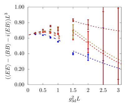
In [10] we then computed $\langle FF\rangle_{\mathrm{NLO}}$, the NLO correction to $Z_{\rm g}^{{\mbox{\tiny\rm{3d}}}}$ in pEQCD; expanded for $m_{\mbox{\tiny\rm{D}}}L\ll 1$ this yields $c_{2}=3/(2\pi^{2})$. In Fig. 1 we show our lattice data for the $\langle EE\rangle$ and $\langle FF\rangle$ channels compared with the pEQCD evaluation and IR ansatz. As one can see, pEQCD and lattice agree at the very least at the smallest separation. We can then merge the two as follows

$\displaystyle Z_{\rm g}^{{\mbox{\tiny\rm{3d}}}}\big{|}^{\text{merge}}=$ $\displaystyle\frac{T}{2}\bigg{\{}\int_{0}^{L_{\mathrm{min}}}{\rm d}L\,L\bigg{[}\langle FF\rangle_{\mathrm{NLO}}-\frac{c_{0}}{L^{3}}-\frac{c_{2}g_{{\mbox{\tiny\rm{3d}}}}^{2}}{L^{2}}\bigg{]}+\int_{L_{\mathrm{min}}}^{L_{\mathrm{max}}}{\rm d}L\,L\bigg{[}\langle FF\rangle_{\mathrm{lat}}-\frac{c_{0}}{L^{3}}\bigg{]}$
$\displaystyle\hskip 14.22636pt+\int_{L_{\mathrm{max}}}^{\infty}{\rm d}L\,L\bigg{[}\langle FF\rangle_{\mathrm{tail}}-\frac{c_{0}}{L^{3}}\bigg{]}\bigg{\}},$ (8)

where $L_{\mathrm{min}}$ and $L_{\mathrm{max}}$ are the smallest and largest separations on the lattice and $\langle FF\rangle_{\mathrm{lat}}$ and $\langle FF\rangle_{\mathrm{tail}}$ are the lattice and IR tail determinations. This procedure can be understood as splitting the integration into three regions: from left to right these are the pEQCD, lattice and IR tail ones. As the $c_{2}$-term is only subtracted in the perturbative region, Eq. (8) introduces an artificial logarithmic dependence on its boundary $L_{\mathrm{min}}$. Further details and numerical results for this procedure are available in [10].

Refer to caption
Refer to caption
Figure 1: Continuum-extrapolated EQCD lattice data on $\langle EE\rangle$ and $\langle FF\rangle$ in eq. (6) with modelled long $L$-tail (short dashes) and NLO pEQCD (long dashes). $L^{3}$ compensates the $c_{0}/L^{3}$ divergence. Figure from [10].

4 Perturbative determination and outlook

\SetWidth1.0\SetScale1.0 \DoubleLine(-10,15)(30,15)1.5 \GluonArc(15,15)(15,0,180)1 2 pi mul 15 mul 360 div 0 180 sub 0 180 sub mul sqrt mul Ldensity mul \GluonArc(15,15)(7.5,0,180)1 2 pi mul 7.5 mul 360 div 0 180 sub 0 180 sub mul sqrt mul Ldensity mul\GCirc(0,15)20.75 \GCirc(30,15)20.75 \Vertex(7.5,15)1 \Vertex(22.5,15)1 (b)subscript\SetWidth1.0\SetScale1.0 \DoubleLine(-10,15)(30,15)1.5 \GluonArc(15,15)(15,0,180)1 2 pi mul 15 mul 360 div 0 180 sub 0 180 sub mul sqrt mul Ldensity mul \GluonArc(15,15)(7.5,0,180)1 2 pi mul 7.5 mul 360 div 0 180 sub 0 180 sub mul sqrt mul Ldensity mul\GCirc(0,15)20.75 \GCirc(30,15)20.75 \Vertex(7.5,15)1 \Vertex(22.5,15)1 𝑏\displaystyle\;\;\parbox[c]{30.0pt}{\begin{picture}(30.0,30.0)(0.0,0.0)\SetWidth{1.0}\SetScale{1.0} \DoubleLine(-10,15)(30,15){1.5} \GluonArc(15,15)(15,0,180){1} {2 pi mul 15 mul 360 div 0 180 sub 0 180 sub mul sqrt mul Ldensity mul} \GluonArc(15,15)(7.5,0,180){1} {2 pi mul 7.5 mul 360 div 0 180 sub 0 180 sub mul sqrt mul Ldensity mul}\GCirc(0,15){2}{0.75} \GCirc(30,15){2}{0.75} \Vertex(7.5,15){1} \Vertex(22.5,15){1} \end{picture}}\;_{(b)}\; \SetWidth1.0\SetScale1.0 \DoubleLine(-10,15)(30,15)1.5 \GluonArc(15,15)(15,0,70)1 2 pi mul 15 mul 360 div 0 70 sub 0 70 sub mul sqrt mul Ldensity mul \GluonArc(15,15)(15,110,180)1 2 pi mul 15 mul 360 div 110 180 sub 110 180 sub mul sqrt mul Ldensity mul \GCirc(15,15 70 sin 15 mul add)50.75 \CArc(15,15 70 sin 15 mul add)(5,0,180) \CArc(15,15 70 sin 15 mul add)(5,180,360)\GCirc(0,15)20.75 \GCirc(30,15)20.75 (c)subscript\SetWidth1.0\SetScale1.0 \DoubleLine(-10,15)(30,15)1.5 \GluonArc(15,15)(15,0,70)1 2 pi mul 15 mul 360 div 0 70 sub 0 70 sub mul sqrt mul Ldensity mul \GluonArc(15,15)(15,110,180)1 2 pi mul 15 mul 360 div 110 180 sub 110 180 sub mul sqrt mul Ldensity mul \GCirc(15,15 70 sin 15 mul add)50.75 \CArc(15,15 70 sin 15 mul add)(5,0,180) \CArc(15,15 70 sin 15 mul add)(5,180,360)\GCirc(0,15)20.75 \GCirc(30,15)20.75 𝑐\displaystyle\;\;\parbox[c]{30.0pt}{\begin{picture}(30.0,30.0)(0.0,0.0)\SetWidth{1.0}\SetScale{1.0} \DoubleLine(-10,15)(30,15){1.5} \GluonArc(15,15)(15,0,70){1} {2 pi mul 15 mul 360 div 0 70 sub 0 70 sub mul sqrt mul Ldensity mul} \GluonArc(15,15)(15,110,180){1} {2 pi mul 15 mul 360 div 110 180 sub 110 180 sub mul sqrt mul Ldensity mul} \GCirc(15,15 70 sin 15 mul add){5}{0.75} \CArc(15,15 70 sin 15 mul add)(5,0,180) \CArc(15,15 70 sin 15 mul add)(5,180,360)\GCirc(0,15){2}{0.75} \GCirc(30,15){2}{0.75} \end{picture}}\;_{(c)}\; \SetWidth1.0\SetScale1.0 \DoubleLine(-10,15)(30,15)1.5 \GluonArc(6,15)(6,0,180)1 2 pi mul 6 mul 360 div 0 180 sub 0 180 sub mul sqrt mul Ldensity mul \GluonArc(24,15)(6,0,180)1 2 pi mul 6 mul 360 div 0 180 sub 0 180 sub mul sqrt mul Ldensity mul\GCirc(0,15)20.75 \GCirc(30,15)20.75 \Vertex(12,15)1 \Vertex(18,15)1 (d1)subscript\SetWidth1.0\SetScale1.0 \DoubleLine(-10,15)(30,15)1.5 \GluonArc(6,15)(6,0,180)1 2 pi mul 6 mul 360 div 0 180 sub 0 180 sub mul sqrt mul Ldensity mul \GluonArc(24,15)(6,0,180)1 2 pi mul 6 mul 360 div 0 180 sub 0 180 sub mul sqrt mul Ldensity mul\GCirc(0,15)20.75 \GCirc(30,15)20.75 \Vertex(12,15)1 \Vertex(18,15)1 subscript𝑑1\displaystyle\;\;\parbox[c]{30.0pt}{\begin{picture}(30.0,30.0)(0.0,0.0)\SetWidth{1.0}\SetScale{1.0} \DoubleLine(-10,15)(30,15){1.5} \GluonArc(6,15)(6,0,180){1} {2 pi mul 6 mul 360 div 0 180 sub 0 180 sub mul sqrt mul Ldensity mul} \GluonArc(24,15)(6,0,180){1} {2 pi mul 6 mul 360 div 0 180 sub 0 180 sub mul sqrt mul Ldensity mul}\GCirc(0,15){2}{0.75} \GCirc(30,15){2}{0.75} \Vertex(12,15){1} \Vertex(18,15){1} \end{picture}}\;_{(d_{1})}\; \SetWidth1.0\SetScale1.0 \DoubleLine(-10,15)(30,15)1.5 \GluonArc(10,15)(10,0,180)1 2 pi mul 10 mul 360 div 0 180 sub 0 180 sub mul sqrt mul Ldensity mul \GluonArc(20,15)(10,180,360)1 2 pi mul 10 mul 360 div 180 360 sub 180 360 sub mul sqrt mul Ldensity mul\GCirc(0,15)20.75 \GCirc(30,15)20.75 \Vertex(10,15)1 \Vertex(20,15)1 (d2)subscript\SetWidth1.0\SetScale1.0 \DoubleLine(-10,15)(30,15)1.5 \GluonArc(10,15)(10,0,180)1 2 pi mul 10 mul 360 div 0 180 sub 0 180 sub mul sqrt mul Ldensity mul \GluonArc(20,15)(10,180,360)1 2 pi mul 10 mul 360 div 180 360 sub 180 360 sub mul sqrt mul Ldensity mul\GCirc(0,15)20.75 \GCirc(30,15)20.75 \Vertex(10,15)1 \Vertex(20,15)1 subscript𝑑2\displaystyle\;\;\parbox[c]{30.0pt}{\begin{picture}(30.0,30.0)(0.0,0.0)\SetWidth{1.0}\SetScale{1.0} \DoubleLine(-10,15)(30,15){1.5} \GluonArc(10,15)(10,0,180){1} {2 pi mul 10 mul 360 div 0 180 sub 0 180 sub mul sqrt mul Ldensity mul} \GluonArc(20,15)(10,180,360){1} {2 pi mul 10 mul 360 div 180 360 sub 180 360 sub mul sqrt mul Ldensity mul}\GCirc(0,15){2}{0.75} \GCirc(30,15){2}{0.75} \Vertex(10,15){1} \Vertex(20,15){1} \end{picture}}\;_{(d_{2})}\; \SetWidth1.0\SetScale1.0 \DoubleLine(30,15)(-10,15)1.5 \GluonArc(15,15)(15,0,180)1 2 pi mul 15 mul 360 div 0 180 sub 0 180 sub mul sqrt mul Ldensity mul \GluonArc(15,15)(15,180,360)1 2 pi mul 15 mul 360 div 180 360 sub 180 360 sub mul sqrt mul Ldensity mul\GCirc(0,15)20.75 \GCirc(30,15)20.75 (e)subscript\SetWidth1.0\SetScale1.0 \DoubleLine(30,15)(-10,15)1.5 \GluonArc(15,15)(15,0,180)1 2 pi mul 15 mul 360 div 0 180 sub 0 180 sub mul sqrt mul Ldensity mul \GluonArc(15,15)(15,180,360)1 2 pi mul 15 mul 360 div 180 360 sub 180 360 sub mul sqrt mul Ldensity mul\GCirc(0,15)20.75 \GCirc(30,15)20.75 𝑒\displaystyle\;\;\parbox[c]{30.0pt}{\begin{picture}(30.0,30.0)(0.0,0.0)\SetWidth{1.0}\SetScale{1.0} \DoubleLine(30,15)(-10,15){1.5} \GluonArc(15,15)(15,0,180){1} {2 pi mul 15 mul 360 div 0 180 sub 0 180 sub mul sqrt mul Ldensity mul} \GluonArc(15,15)(15,180,360){1} {2 pi mul 15 mul 360 div 180 360 sub 180 360 sub mul sqrt mul Ldensity mul}\GCirc(0,15){2}{0.75} \GCirc(30,15){2}{0.75} \end{picture}}\;_{(e)}\;
\SetWidth1.0\SetScale1.0 \DoubleLine(-10,15)(30,15)1.5 \GluonArc(15,15)(15,0,90)1 2 pi mul 15 mul 360 div 0 90 sub 0 90 sub mul sqrt mul Ldensity mul \GluonArc(15,15)(15,90,180)1 2 pi mul 15 mul 360 div 90 180 sub 90 180 sub mul sqrt mul Ldensity mul \Gluon(15,30)(15,15)1 15 15 sub 15 15 sub mul 30 15 sub 30 15 sub mul add sqrt Ldensity mul\GCirc(0,15)20.75 \GCirc(30,15)20.75 \Vertex(15,15)1 (f)subscript\SetWidth1.0\SetScale1.0 \DoubleLine(-10,15)(30,15)1.5 \GluonArc(15,15)(15,0,90)1 2 pi mul 15 mul 360 div 0 90 sub 0 90 sub mul sqrt mul Ldensity mul \GluonArc(15,15)(15,90,180)1 2 pi mul 15 mul 360 div 90 180 sub 90 180 sub mul sqrt mul Ldensity mul \Gluon(15,30)(15,15)1 15 15 sub 15 15 sub mul 30 15 sub 30 15 sub mul add sqrt Ldensity mul\GCirc(0,15)20.75 \GCirc(30,15)20.75 \Vertex(15,15)1 𝑓\displaystyle\;\;\parbox[c]{30.0pt}{\begin{picture}(30.0,30.0)(0.0,0.0)\SetWidth{1.0}\SetScale{1.0} \DoubleLine(-10,15)(30,15){1.5} \GluonArc(15,15)(15,0,90){1} {2 pi mul 15 mul 360 div 0 90 sub 0 90 sub mul sqrt mul Ldensity mul} \GluonArc(15,15)(15,90,180){1} {2 pi mul 15 mul 360 div 90 180 sub 90 180 sub mul sqrt mul Ldensity mul} \Gluon(15,30)(15,15){1} {15 15 sub 15 15 sub mul 30 15 sub 30 15 sub mul add sqrt Ldensity mul}\GCirc(0,15){2}{0.75} \GCirc(30,15){2}{0.75} \Vertex(15,15){1} \end{picture}}\;_{(f)}\; \SetWidth1.0\SetScale1.0 \DoubleLine(-10,15)(30,15)1.5 \GluonArc(15,15)(15,0,90)1 2 pi mul 15 mul 360 div 0 90 sub 0 90 sub mul sqrt mul Ldensity mul \GluonArc(15,15)(15,90,180)1 2 pi mul 15 mul 360 div 90 180 sub 90 180 sub mul sqrt mul Ldensity mul \GluonArc(0,30)(15,270,360)1 2 pi mul 15 mul 360 div 270 360 sub 270 360 sub mul sqrt mul Ldensity mul \GCirc(0,15)20.75 \GCirc(30,15)20.75 (g)subscript\SetWidth1.0\SetScale1.0 \DoubleLine(-10,15)(30,15)1.5 \GluonArc(15,15)(15,0,90)1 2 pi mul 15 mul 360 div 0 90 sub 0 90 sub mul sqrt mul Ldensity mul \GluonArc(15,15)(15,90,180)1 2 pi mul 15 mul 360 div 90 180 sub 90 180 sub mul sqrt mul Ldensity mul \GluonArc(0,30)(15,270,360)1 2 pi mul 15 mul 360 div 270 360 sub 270 360 sub mul sqrt mul Ldensity mul \GCirc(0,15)20.75 \GCirc(30,15)20.75 𝑔\displaystyle\;\;\parbox[c]{30.0pt}{\begin{picture}(30.0,30.0)(0.0,0.0)\SetWidth{1.0}\SetScale{1.0} \DoubleLine(-10,15)(30,15){1.5} \GluonArc(15,15)(15,0,90){1} {2 pi mul 15 mul 360 div 0 90 sub 0 90 sub mul sqrt mul Ldensity mul} \GluonArc(15,15)(15,90,180){1} {2 pi mul 15 mul 360 div 90 180 sub 90 180 sub mul sqrt mul Ldensity mul} \GluonArc(0,30)(15,270,360){1} {2 pi mul 15 mul 360 div 270 360 sub 270 360 sub mul sqrt mul Ldensity mul} \GCirc(0,15){2}{0.75} \GCirc(30,15){2}{0.75} \end{picture}}\;_{(g)}\; \SetWidth1.0\SetScale1.0 \DoubleLine(-10,15)(30,15)1.5 \GluonArc(15,15)(15,0,180)1 2 pi mul 15 mul 360 div 0 180 sub 0 180 sub mul sqrt mul Ldensity mul \GluonArc(7.5,15)(7.5,0,180)1 2 pi mul 7.5 mul 360 div 0 180 sub 0 180 sub mul sqrt mul Ldensity mul\GCirc(0,15)20.75 \GCirc(30,15)20.75 \Vertex(15,15)1 (h)subscript\SetWidth1.0\SetScale1.0 \DoubleLine(-10,15)(30,15)1.5 \GluonArc(15,15)(15,0,180)1 2 pi mul 15 mul 360 div 0 180 sub 0 180 sub mul sqrt mul Ldensity mul \GluonArc(7.5,15)(7.5,0,180)1 2 pi mul 7.5 mul 360 div 0 180 sub 0 180 sub mul sqrt mul Ldensity mul\GCirc(0,15)20.75 \GCirc(30,15)20.75 \Vertex(15,15)1 \displaystyle\;\;\parbox[c]{30.0pt}{\begin{picture}(30.0,30.0)(0.0,0.0)\SetWidth{1.0}\SetScale{1.0} \DoubleLine(-10,15)(30,15){1.5} \GluonArc(15,15)(15,0,180){1} {2 pi mul 15 mul 360 div 0 180 sub 0 180 sub mul sqrt mul Ldensity mul} \GluonArc(7.5,15)(7.5,0,180){1} {2 pi mul 7.5 mul 360 div 0 180 sub 0 180 sub mul sqrt mul Ldensity mul}\GCirc(0,15){2}{0.75} \GCirc(30,15){2}{0.75} \Vertex(15,15){1} \end{picture}}\;_{(h)}\; \SetWidth1.0\SetScale1.0 \DoubleLine(-10,15)(30,15)1.5 \GluonArc(0,22.5)(7.5,-90,270)1 2 pi mul 7.5 mul 360 div -90 270 sub -90 270 sub mul sqrt mul Ldensity mul \GluonArc(30,22.5)(7.5,-90,270)1 2 pi mul 7.5 mul 360 div -90 270 sub -90 270 sub mul sqrt mul Ldensity mul\GCirc(0,15)20.75 \GCirc(30,15)20.75 (i)subscript\SetWidth1.0\SetScale1.0 \DoubleLine(-10,15)(30,15)1.5 \GluonArc(0,22.5)(7.5,-90,270)1 2 pi mul 7.5 mul 360 div -90 270 sub -90 270 sub mul sqrt mul Ldensity mul \GluonArc(30,22.5)(7.5,-90,270)1 2 pi mul 7.5 mul 360 div -90 270 sub -90 270 sub mul sqrt mul Ldensity mul\GCirc(0,15)20.75 \GCirc(30,15)20.75 𝑖\displaystyle\;\;\parbox[c]{30.0pt}{\begin{picture}(30.0,30.0)(0.0,0.0)\SetWidth{1.0}\SetScale{1.0} \DoubleLine(-10,15)(30,15){1.5} \GluonArc(0,22.5)(7.5,-90,270){1} {2 pi mul 7.5 mul 360 div -90 270 sub -90 270 sub mul sqrt mul Ldensity mul} \GluonArc(30,22.5)(7.5,-90,270){1} {2 pi mul 7.5 mul 360 div -90 270 sub -90 270 sub mul sqrt mul Ldensity mul}\GCirc(0,15){2}{0.75} \GCirc(30,15){2}{0.75} \end{picture}}\;_{(i)}\; \SetWidth1.0\SetScale1.0 \DoubleLine(-10,15)(30,15)1.5 \GluonArc(0,22.5)(7.5,-90,270)1 2 pi mul 7.5 mul 360 div -90 270 sub -90 270 sub mul sqrt mul Ldensity mul \GluonArc(22.5,15)(7.5,0,180)1 2 pi mul 7.5 mul 360 div 0 180 sub 0 180 sub mul sqrt mul Ldensity mul\GCirc(0,15)20.75 \GCirc(30,15)20.75 \Vertex(15,15)1 (j)subscript\SetWidth1.0\SetScale1.0 \DoubleLine(-10,15)(30,15)1.5 \GluonArc(0,22.5)(7.5,-90,270)1 2 pi mul 7.5 mul 360 div -90 270 sub -90 270 sub mul sqrt mul Ldensity mul \GluonArc(22.5,15)(7.5,0,180)1 2 pi mul 7.5 mul 360 div 0 180 sub 0 180 sub mul sqrt mul Ldensity mul\GCirc(0,15)20.75 \GCirc(30,15)20.75 \Vertex(15,15)1 𝑗\displaystyle\;\;\parbox[c]{30.0pt}{\begin{picture}(30.0,30.0)(0.0,0.0)\SetWidth{1.0}\SetScale{1.0} \DoubleLine(-10,15)(30,15){1.5} \GluonArc(0,22.5)(7.5,-90,270){1} {2 pi mul 7.5 mul 360 div -90 270 sub -90 270 sub mul sqrt mul Ldensity mul} \GluonArc(22.5,15)(7.5,0,180){1} {2 pi mul 7.5 mul 360 div 0 180 sub 0 180 sub mul sqrt mul Ldensity mul}\GCirc(0,15){2}{0.75} \GCirc(30,15){2}{0.75} \Vertex(15,15){1} \end{picture}}\;_{(j)}\;
Figure 2: Diagrams contributing to $Z_{\rm g}$ at LO and NLO. Gray shaded vertices denote $F^{-\perp}$ insertions; a solid line a Wilson line; and a curly line a gluon, with the blob its self-energy. See [10] for the EQCD counterpart.

To lift this artificial cutoff dependence on $L_{\mathrm{min}}$, in [19] we set out to determine the two-loop contribution to $Z_{\rm g}$ in thermal 4D QCD for loop four-momenta of order $T$. In principle this requires the evaluation of diagrams $(b)$ $(j)$ in Fig. 4. Using the equation of motion of the Wilson line, we can show that only diagram $(c)$ contributes in Feynman gauge.

There we identify the IR-divergent contribution as arising from a thermal momentum, $K\sim T$ in the blob and a soft one in the outer integration, $Q\sim gT$. We carefully evaluate it in dimensional regularization; we do the same for the $-c_{2}g_{{\mbox{\tiny\rm{3d}}}}^{2}\theta(L_{\mathrm{min}}-L)/L^{2}$ subtraction in Eq. (8), finding that UV and IR poles cancel as expected, yielding this new matching term [19]

$$Z_{\rm g}^{\mathrm{match}}=\frac{3g^{2}T^{2}}{4\pi^{2}}\bigg{[}\ln(2L_{\mathrm{min}}T)+{\gamma_{\mbox{\tiny\rm{E}}}}-\frac{3}{2}\bigg{]}\,,\qquad Z_{\rm g}^{\text{non-pert class}}=Z_{\rm g}^{{\mbox{\tiny\rm{3d}}}}\big{|}^{\text{merge}}+Z_{\rm g}^{\mathrm{match}}\,.$$ (9)

The $\ln(L_{\mathrm{min}})$ dependence vanishes in $Z_{\rm g}^{\text{non-pert class}}$, the sum of Eq. (8) and $Z_{\rm g}^{\mathrm{match}}$. $Z_{\rm g}^{\text{non-pert class}}$ thus provides the complete non-perturbative determination of the classical contribution to $Z_{\rm g}$. Numerically, this combination results in a negative contribution to $Z_{\rm g}$ which is in magnitude larger than the negative $Z_{\rm g}\big{|}^{\mathrm{NLO}}=-Tm_{\mbox{\tiny\rm{D}}}/(2\pi)$. Physically, negativity can be understood as follows. Let us consider the soft sector of bare 4D QCD. At LO Eq. (4) implies $Z_{\rm g}|^{\text{soft}}_{\text{bare LO}}=\frac{1}{\pi^{2}}\int_{gT}{\rm d}q\,q\,T/q$. Our procedure amounts to subtracting this bare soft sector and replacing it with its screened EQCD counterpart, which reduces its contribution.

Before conclusions on the convergence of this EQCD approach can be drawn, it must be noted that $Z_{\rm g}^{\mathrm{match}}$ only contains the part of the two-loop 4D QCD calculation responsible for the IR limit, and that this separation is to some degree arbitrary. Only the full determination of the two-loop 4D QCD contribution to $Z_{\rm g}$ will allow a definite conclusion.111This is a distinct problem from the one recently tackled in [22, 23, 24], namely the two-loop and power corrections to Hard Thermal Loops and their relation to the asymptotic mass for quasiparticles obeying $T\gg p\gg gT$. Preliminary results [19] further indicate the likely emergence of collinear modes at this order in perturbation theory. These modes have energies of order $E$ at small angles to $\bm{p}$, see [25] for the interplay of collinear and classical modes in transverse momentum broadening.

Acknowledgments

JG acknowledges support by a PULSAR grant from the Région Pays de la Loire and by the Agence Nationale de la Recherche under grant ANR-22-CE31-0018 (AUTOTHERM). PS was supported by the European Research Council, grant no. 725369 and by the Academy of Finland, grant no. 1322507. PS and GM were supported by the Deutsche Forschungsgemeinschaft (DFG, German Research Foundation) through the CRC-TR 211 ‘Strong-interaction matter under extreme conditions’ – project number 315477589 – TRR 211.

References