Nested Elimination:
A Simple Algorithm for Best-Item Identification from Choice-Based Feedback

Abstract

We study the problem of best-item identification from choice-based feedback. In this problem, a company sequentially and adaptively shows display sets to a population of customers and collects their choices. The objective is to identify the most preferred item with the least number of samples and at a high confidence level. We propose an elimination-based algorithm, namely Nested Elimination (NE), which is inspired by the nested structure implied by the information-theoretic lower bound. NE is simple in structure, easy to implement, and has a strong theoretical guarantee for sample complexity. Specifically, NE utilizes an innovative elimination criterion and circumvents the need to solve any complex combinatorial optimization problem. We provide an instance-specific and non-asymptotic bound on the expected sample complexity of NE. We also show NE achieves high-order worst-case asymptotic optimality. Finally, numerical experiments from both synthetic and real data corroborate our theoretical findings.

1 Introduction

Online machine learning (Shalev-Shwartz et al., 2012) has been proven to be an effective method for efficiently collecting and utilizing large amounts of data, as evidenced by theoretical and practical studies. In this paper, we investigate the online learning problem of best-item identification from choice-based feedback akin to Feng et al. (2021), which is a practical extension of the stochastic multi-armed bandit problem (Lattimore & Szepesvári, 2020).

Our problem can be applied to a wide range of contemporary real-world scenarios. The following example will be used throughout this paper for clarity and readability. Consider a company that seeks to identify the most preferred item (e.g., commercial product) among a set of alternative options. The company can interact with customers through a feedback collection process to learn the unknown preference. In particular, the company sequentially displays (possibly) different subsets of items to different customers and asks them to choose their favorite within the display sets. The subsequent display sets may depend on prior ones as well as the previously obtained samples. For the company, an important objective is to minimize the cost of feedback collection while maintaining a high level of accuracy in identifying the top-ranked item.

To address the company’s problem, Feng et al. (2021) proposed a relatively general framework for encoding customers’ preferences using their choice probabilities. They assumed that customers’ preferences (i.e., choice probability distributions) satisfy certain consistency and separability conditions, i.e., the more preferred item is always chosen with (strictly) higher probabilities. On account of the instance-specific information-theoretical lower bound, they proposed a minimax formulation of the company’s problem and designed a randomized policy, called Myopic Tracking Policy (or MTP), which is worst-case asymptotically optimal. However, some limitations of MTP still need to be addressed urgently. One major issue is its computational inefficiency for large-scale problems, which requires solving combinatorial optimization problems. Additionally, the theoretical guarantees of MTP are not only asymptotic in nature but also instance-independent.

Main Contributions.

Our main results and contributions are summarized as follows:

1. We design an elimination-based algorithm Nested Elimination (NE); see Section 3. This algorithm is based on a new design of a sequence of hitting times governing when (and how) to rule out sub-optimal items. This design is inspired by the nested structure in the optimal solution to the max-min problem for the information-theoretic lower bound. It differs from many classic successive elimination algorithms for multi-armed bandit problems, typically based on estimating the expected reward of each arm (Even-Dar et al., 2006; Kalyanakrishnan & Stone, 2010; Karnin et al., 2013). It is also different from those inspired by the information-theoretic lower bound and based on the track-and-plug-in strategies (Chernoff, 1959; Garivier & Kaufmann, 2016; Feng et al., 2021).

   In addition, The algorithm is rather simple in structure and quick to implement, as the elimination criterion is easily calculable. In particular, our algorithm differs from MTP in that it does not involve any combinatorial optimization problems, making it efficient computationally and suitable for large-scale applications.

2. We theoretically analyze the performance of our algorithm NE from multiple perspectives; see Section 4. To summarize, for every (instead of just worst-case) instances and error tolerance $\delta$, we provide a non-asymptotic and instance-specific bound of the expected sample complexity of NE; see Theorem 4.1. This performance guarantee is always better than that of MTP, and sometimes the difference can be on the order of $\Omega(\log(1/\delta))$.

   Apart from tight performance characterization, we also show higher-order worst-case optimality of NE. Specifically, under the worst-case instances, the difference between the sample complexity under NE and the information-theoretical lower bound is bounded by a constant independent of $\delta$; see Proposition 4.2 and discussion thereafter. In comparison, MTP by Feng et al. (2021) allows the residual term to be on the order of $o(\log(1/\delta))$.

3. We conduct comprehensive numerical experiments generated from both synthetic and real data sets; see Section 5. In particular, we demonstrate both the computational and sample efficiency of NE, especially compared with MTP.

More Related Work.

Our work is also related to the stochastic multi-armed bandit problem, which was first introduced by Thompson (1933). The multi-armed bandit model offers a straightforward yet effective online learning framework, which has been studied extensively in the literature. While the regret minimization problem aims at maximizing the cumulative reward by carefully balancing the trade-off between exploration and exploitation (Auer et al., 2002; Bubeck & Cesa-Bianchi, 2012; Agrawal & Goyal, 2012), the pure exploration problem focuses on achieving efficient exploration with specific objectives in mind, e.g., best arm identification (Even-Dar et al., 2006; Audibert et al., 2010; Karnin et al., 2013; Garivier & Kaufmann, 2016). For a more in-depth review of bandit algorithms, we refer to Lattimore & Szepesvári (2020).

Our studied model differs from standard multi-armed bandits, as the decision variable is a subset of items referred to as a display set, instead of a single item, and the observation is an item rather than a stochastic reward. Therefore, we refrain from using the terminology “arm” to prevent ambiguity. However, there is another line of work that incorporates the choice-based feedback model into multi-armed bandits. In particular, Chen et al. (2018) studied the problem of top-items identification under a Luce-type choice model, which is different from the class of choice models we consider in this work, as described in Section 2. Additionally, when evaluating the asymptotic performance of their algorithm, they fixed the moderate confidence level while allowing other instance-specific parameters (such as the number of items) to tend to infinity. In contrast, we fix the instance and let the confidence level tend to zero, which is more commonly adopted in the literature on pure exploration. Furthermore, Saha & Gopalan (2020) considered the problem of identifying a near-optimal item under a random utility-based discrete choice model, where each item is associated with an unknown random utility score. Nevertheless, they fixed the size of the display sets, whereas we allow for display sets of varying sizes. Finally, we remark that, to the best of our knowledge, only the results in Feng et al. (2021) are comparable to ours.

2 Problem Setup and Preliminaries

Choice-Based Feedback Model.

We consider a choice-based feedback model in which a customer randomly selects exactly one item from the display set presented by the company (or agent). In particular, the set of available items is denoted as $[K]:=\{1,2,\ldots,K\}$ and the collection of all the possible display sets is $\mathcal{S}:=\{S\subset[K],|S|\geq 2\}$. Therefore, an instance of such a choice-based feedback model corresponds to an inherent preference $f$, which can be described by the probability $f(i|S)$ that item $i$ is chosen from the display set $S$ for any $S\in\mathcal{S}$ and $i\in S$.

We follow the notation of Feng et al. (2021) and only assume that preference $f$ belongs to the $p$-Separable family $\mathcal{M}_{p}$ for some given $p\in(0,1)$; see Definition 2.1.

Definition 2.1 ($p$-Separable family).

Let $p\in(0,1)$ be a fixed dispersion parameter. A preference $f$ belongs to the $p$-Separable family $\mathcal{M}_{p}$ if:

1. For any $S\in\mathcal{S}$, $f(i|S)>0$ if and only if $i\in S$;

2. For any $S\in\mathcal{S}$, $\sum_{i\in S}f(i|S)=1$;

3. There exists a global ranking $\sigma_{f}:[K]\to[K]$ such that for any $S\in\mathcal{S}$ and $i,i^{\prime}\in S$, $f(i|S)\leq pf(i^{\prime}|S)$ if $\sigma_{f}(i^{\prime})<\sigma_{f}(i)$.

For any $S\in\mathcal{S}$ and $i\in S$, we refer to the local ranking of $i$ in $S$ as $\sigma_{f}(i|S):=\sum_{j\in S}\mathbbm{1}\{\sigma_{f}(i)\leq\sigma_{f}(j)\}$. For the convenience of expression, we assume that the unknown global ranking $\sigma_{f}$ of the customer preference $f$ that interacts with the company is the identity ranking $\sigma_{*}:=(1,2,\ldots,K)$ throughout this work, without loss of generality. Accordingly, item $1$ is always the customer’s most preferred item within the item set $[K]$.

Remark 2.2.

The reason we adopt the $p$-Separable family $\mathcal{M}_{p}$ of preference instances as our modeling framework is that it is relatively general. Essentially, we assume that the choice probabilities corresponding to $f$ are (statistically) consistent with some (unknown) ranking of items. In addition, the choice probabilities are separable by at least a factor of $p$. Many common choice models, such as the multinomial logit (MNL) model and the Mallows choice model, could be incorporated into this framework. See Remark 2 of Feng et al. (2021) for more discussion.

Remark 2.3.

The parameter $p$ measures the noise level of the choice-based feedback model and is also a separation parameter. Throughout the paper, we perform our analysis treating the value of $p$ as known and given. However, note that $\mathcal{M}_{p}\subset\mathcal{M}_{p^{\prime}}$ for all $p<p^{\prime}$. Therefore, if only a conservative estimate (i.e., an upper bound) of $p$, say, $p^{\prime}$ is available, our theoretical results for the algorithm performance (e.g., Theorem 4.1, as well as the worst-case asymptotic optimality (9)) still hold after replacing $p$ with $p^{\prime}$.

Best-Item Identification from Choice-Based Feedback.

The company aims to identify the best item by displaying subsets of the item set $[K]$ to customers with an unknown consensus preference $f$ sequentially and adaptively. Specifically, at each time step $t\in\mathbb{N}^{+}:=\{1,2,3,\ldots\}$, the company chooses one display set $S_{t}\in\mathcal{S}$ and presents it to one customer. Then the customer selects an item $X_{t}\in S_{t}$ according to the underlying probability distribution $f(\cdot|S_{t})$.

More formally, the company uses an online policy $\pi$ to decide the display set $S_{t}$ to present at each time step $t$, to select a time $\tau$ to stop the interactions, and to ultimately recommend $i_{\mathrm{out}}$ as the identified best item to output. Let $\mathcal{F}_{t}:=\sigma(S_{1},X_{1},\ldots,S_{t},X_{t})$ denote the smallest $\sigma$-field generated by the history of display sets and customers’ choices up to and including time $t$. Therefore, the online algorithm $\pi$ is comprised of three components:

• The display rule selects $S_{t}$ (with possible randomization), which is adapted to the filtration $\mathcal{F}_{t-1}$;

• The stopping rule determines a stopping time $\tau$, which is adapted to the filtration $(\mathcal{F}_{t})_{t=1}^{\infty}$;

• The recommendation rule produces a candidate best item $i_{\mathrm{out}}$, which is $\mathcal{F}_{\tau}$-measurable.

To facilitate comparisons with previous work, we will also adopt the fixed-confidence setting in the theoretical analysis. In the fixed-confidence setting, a confidence level $\delta\in(0,1)$ is given. Then the company is required to identify the best item with probability at least $1-\delta$ using the fewest time steps (i.e., samples).

Definition 2.4 ($\delta$-PAC policy).

For a prescribed confidence level $\delta\in(0,1)$, an online best-item identification policy $\pi$ is said to be $\delta$-PAC (probably approximately correct) if for all preferences $f\in\mathcal{M}_{p}$, it terminates within a finite time almost surely and the probability of error is no more than $\delta$ (i.e., $\mathbb{P}(\tau<\infty)=1$ and $\mathbb{P}(i_{\mathrm{out}}\neq 1)\leq\delta$). Furthermore, for a class of policies $\Pi=\{\pi_{\delta}\}_{\delta\in(0,1)}$ parameterized by $\delta$, we say it is PAC if $\pi_{\delta}$ is $\delta$-PAC for all $\delta$.

In this regard, our overarching goal is to design a $\delta$-PAC best-item identification policy while minimizing its expected sample complexity $\operatorname{\mathbb{E}}[\tau]$.

Information-Theoretic Lower Bound and Worst-Case Analysis.

Following an argument that dates back to Chernoff (1959), which was further popularized by Kaufmann et al. (2016), one can derive an information-theoretic lower bound on $\operatorname{\mathbb{E}}[\tau]$ in terms of the optimal value of a certain max-min optimization problem. Let $\mathcal{P}(\mathcal{S})$ denote the collection of all the probability distributions on $\mathcal{S}$. For any fixed preference $f\in\mathcal{M}_{p}$, we define $\overline{\mathcal{M}}_{p}(f):=\{f^{\prime}\in\mathcal{M}_{p}:\sigma_{f^{\prime}}(1)\neq\sigma_{f}(1)\}$, which represents the set of alternative preferences with different best items. We summarize the non-asymptotic and instance-specific lower bound on $\operatorname{\mathbb{E}}[\tau]$ in Theorem 2.5 below.

Theorem 2.5 (Paraphrased from Feng et al., 2021).

For any preference $f\in\mathcal{M}_{p}$, let

$$I_{*}(f):=\sup_{\lambda\in\mathcal{P}(\mathcal{S})\!}\inf_{f^{\prime}\in\overline{\mathcal{M}}_{p}(f)}\!\sum_{S\in\mathcal{S},i\in S}\lambda(S)f(i|S)\log\tfrac{f(i|S)}{f^{\prime}(i|S)}.$$ (1)

Then any $\delta$-PAC best-item identification policy satisfies

$$\operatorname{\mathbb{E}}[\tau]\geq\frac{\log(1/\delta)-\log 2.4}{I_{*}(f)}.$$

In the information-theoretical lower bound, $I_{*}(\cdot)$ is a measure that quantifies the easiness of identifying the best item from the item set $[K]$. The optimal solution $\lambda^{\ast}$ to the outer maximization problem (1) can be roughly interpreted as the optimal long-run-average proportions of different display sets to be presented. Therefore, it can be used to inspire designs of efficient algorithms; see Chernoff (1959), Garivier & Kaufmann (2016).

However, in our case, the prohibitive complexity of the problem (1) makes it impractical to utilize $I_{*}(\cdot)$ directly. In this regard, Feng et al. (2021) identified a “hardest-to-learn” preference instance (uniquely specified up to permutation), which is referred to as $f^{\mathrm{OA}}$. Here the superscript “OA” refers to Ordinal Attraction (OA) preferences; see Remark 2.6. The instance $f^{\mathrm{OA}}$ minimizes the hardness quantity $I_{*}(\cdot)$ among $\mathcal{M}_{p}$. In other words,

$$I_{*}^{\mathrm{OA}}:=I_{*}(f^{\mathrm{OA}})=\min_{f\in\mathcal{M}_{p}}I_{*}(f).$$ (2)

It turns out that the problem (1) is solvable under $f^{\mathrm{OA}}$. In particular, Feng et al. (2021) found that when $f=f^{\mathrm{OA}}$, the optimal solution $\lambda^{\ast}$ to the outer maximization problem of (1) admits a nested structure. That is, $\lambda^{*}(S)>0$ if and only if $S\in\mathcal{\{}[i]:i=2,\ldots,K\}$.

Feng et al. (2021) designed a randomized strategy (i.e., MTP) specialized to the worst-case instances $\mathcal{M}_{p}^{\mathrm{OA}}$ by trying to match the randomization distribution with $\lambda^{*}$ using a track-and-plug-in strategy. They showed that MTP is worst-case asymptotically optimal, i.e.,

$$\textsc{MTP}\in\operatorname*{arg\,min}_{\Pi\text{ is }\text{PAC}}\ \ \sup_{f\in\mathcal{M}_{p}}\ \ \limsup_{\delta\downarrow 0}\ \ \tfrac{\mathbb{E}^{\pi_{\delta}}_{f}[\tau]}{\log(1/\delta)}.$$ (3)

In comparison, we will directly exploit the nested structure in $\lambda^{*}$ and design a nested elimination-based algorithm; see Section 3 for the details.

Remark 2.6.

The closed form expression for $f^{\mathrm{OA}}$ is that $f^{\mathrm{OA}}(i|S)=\frac{1-p}{1-p^{|S|}}p^{\sigma_{\!f^{\scalebox{0.5}{\mbox{$\displaystyle\mathrm{OA}$}}}}\!(i|S)-1}$ for all $S\in\mathcal{S}$ and $i\in S$. Under this preference instance, the choice probability of an item only depends on its ordinal information, i.e., its local ranking within the display set. That is where the name “Ordinal Attraction” (OA) comes from. As such, it is an extension of commonly-used noisy pairwise comparison models (Braverman & Mossel, 2008; Wauthier et al., 2013). Interestingly, Feng & Tang (2022) also showed that $f^{\mathrm{OA}}$ could also be viewed as the aggregate choice model from a distance-based ranking distribution, therefore “rationalizing” this choice model from a different perspective.

Other Notations.

For any display set $S\in\mathcal{S}$ and its subset $S^{\prime}\subset S$, we define $f(S^{\prime}|S):=\sum_{i\in S^{\prime}}f(i|S)$, which is the probability that a customer with preference $f$ chooses one item in the subset $S^{\prime}$ when presented with display set $S$. Consider any multivariate function $g:\mathbb{R}\times\mathbb{R}^{n-1}\to\mathbb{R}$, and any univariate function $h:\mathbb{R}\to\mathbb{R}$. For any fixed $y\in\mathbb{R}^{n-1}$, we say $g(x,y)=O_{x}(h(x))$ (resp. $\Omega_{x}(h(x))$) if there exists a positive constant $c$ and a constant $x_{0}$ (possibly dependent on parameter $y$) such that $|g(x,y)|\leq c\cdot h(x)$ (resp. $|g(x,y)|\geq c\cdot h(x)$) for all $x\geq x_{0}$. Alternatively, we say $g(x,y)=o_{x}(h(x))$ (resp. $\omega_{x}(h(x))$) if for any positive constant $c$, there exists a constant $x_{0}$ (possibly dependent on parameter $y$) such that $|g(x,y)|<c\cdot h(x)$ (resp. $|g(x,y)|>c\cdot h(x)$) for all $x\geq x_{0}$.

3 The Nested Elimination Algorithm

In this section, we propose a structurally simple and computationally efficient algorithm, namely Nested Elimination (or NE), to identify the best item from choice-based feedback. The pseudocode for NE is presented in Algorithm 1 and explained in the following.

Algorithm 1 Nested Elimination (NE)

Input: Tuning parameter $M>0.$

1:  Initialize voting score $W_{0}(i)\leftarrow 0$ for all $i\in[K]$, active item set $S_{\mathrm{active}}\leftarrow[K]$, $t\leftarrow 0$.

2:  while $|S_{\mathrm{active}}|>1$ do

3:     Update the timer: $t\leftarrow t+1$.

4:     Display the active set $S_{\mathrm{active}}$, and observe the choice $X_{t}\in S_{\mathrm{active}}$.

5:     Update voting scores based on $X_{t}$:

$$W_{t}(i)\leftarrow\begin{cases}W_{t-1}(i)+1&\text{if }i=X_{t}\\ W_{t-1}(i)&\text{if }i\neq X_{t}.\\ \end{cases}$$

6:     Update the active set: (i) Sort the remaining items based on their voting scores. That is, find a ranking $\sigma_{t}:[|S_{\mathrm{active}}|]\to S_{\mathrm{active}}$ such that $W_{t}(\sigma_{t}(1))\geq W_{t}(\sigma_{t}(2))\geq\cdots\geq W_{t}(\sigma_{t}(|S_{\mathrm{active}}|))$. (ii) Search for the smallest $k$ such that

$$\sum\nolimits_{i=1}^{k}W_{t}(\sigma_{t}(i))-kW_{t}(\sigma_{t}(k+1))\geq M.$$

     If such $k$ exists, $S_{\mathrm{active}}\leftarrow\{\sigma_{t}(1),\ldots,\sigma_{t}(k)\}$.

7:  end while

Output: The only element $i_{\mathrm{out}}$ of $S_{\mathrm{active}}$.

As its name suggests, our algorithm NE is elimination-based and maintains an active item set $S_{\mathrm{active}}$ at each time step. The algorithm is parameterized by a tuning parameter $M>0$, which plays an essential role in controlling the accuracy of the eliminations. We will discuss more on the choice of parameter $M$ in Theorem  4.1. As a general rule, the larger the parameter $M$, the more effective the eliminations are in preserving the best item. This, in turn, leads to a lower probability of outputting suboptimal items.

Initially, all the items are included in the active item set $S_{\mathrm{active}}$. For any item $i\in[K]$, we refer to the number of times that item $i$ is selected by the customers up to time $t$ as voting score $W_{t}(i)$.

At each time step $t$, NE displays $S_{\mathrm{active}}$ to the next customer, and observes the choice $X_{t}\in S_{\mathrm{active}}$. After that, the algorithm sorts the active items with respect to their voting scores so that the $i^{\mathrm{th}}$ most voted item up to time $t$ is denoted by $W_{t}(\sigma_{t}(i))$ for any $i\in[|S_{\mathrm{active}}|]$.

Our elimination criterion in Step 6 (ii) is straightforward to implement. Specifically, we retain only the $k$ items with the highest voting scores in $S_{\mathrm{active}}$ if they satisfy the following condition:

$$\sum\nolimits_{i=1}^{k}W_{t}(\sigma_{t}(i))-kW_{t}(\sigma_{t}(k+1))\geq M.$$ (4)

Furthermore, if multiple values of $k$ meet this condition, we select the smallest one to facilitate the algorithm procedure.

As the algorithm progresses, there is only one single item $i_{\mathrm{out}}$ in the active item set $S_{\mathrm{active}}$ eventually. That will be the output of our algorithm NE.

Remark 3.1.

One main observation we make from NE is that at every stage (i.e., time steps between item eliminations), the “active” voting scores $\{W_{t}(i):i\in S_{active}\}$ behave like a (biased) random walk on the integer lattice $\mathbb{Z}^{|S_{active}|}$. In the meantime, the elimination criterion follows a sequence of hitting times of the corresponding random walk. This structure gives us great analytical tractability by leveraging tools such as martingale theory, and that is how non-asymptotic bounds are possible for us.

Remark 3.2.

On a more technical note, multiple items can be eliminated within a single time step under Algorithm 1. In this regard, it is straightforward to verify that if there exists some value of $k$ such that the elimination criterion is satisfied, i.e., $\sum_{i=1}^{k}W_{t}(\sigma_{t}(i))-kW_{t}(\sigma_{t}(k+1))\geq M$, then for all integer $k^{\prime}\in[k,|S_{\mathrm{active}}|-1]$,

$$\sum\nolimits_{i=1}^{k^{\prime}}W_{t}(\sigma_{t}(i))-k^{\prime}W_{t}(\sigma_{t}(k^{\prime}+1))\geq M.$$

Thus, the outcomes of the eliminations will not be altered if we only allow eliminating the items one by one, starting with the least voted item, still within one time step. This is more convenient for the analysis presented in Section 4, although it requires slightly more calculations. See Algorithm 2 in the appendix for the pseudocode of such formulation.

4 Main Results

In this section, we theoretically analyze the correctness and sample complexity (stopping time) of our algorithm NE (Algorithm 1). For ease of reading, we assume that the tuning parameter $M$ is an integer without loss of generality. In general situations, $M$ appearing in the analysis should be replaced by $\lceil M\rceil$, without affecting other expressions.

For any preference $f\in\mathcal{M}_{p}$, we introduce a novel hardness quantity

$${I^{\mathrm{N}}(f)}:=\log\left(\tfrac{1}{p}\right)\left[\sum\nolimits_{r=1}^{K-1}D(f,r)\right]^{-1},$$

where the detailed expressions of $D(f,r)$ for all $r\in[K-1]$ are deferred to Appendix B. In addition, we define $\beta(K):=2^{K-1}-1$ for simplicity, which is a constant independent of $\delta$. We now present our first main result in Theorem 4.1 below.

Theorem 4.1 (Sample complexity of NE in the fixed-confidence setting).

For every confidence level $\delta\in(0,1)$, NE is $\delta$-PAC with parameter

$$M=\frac{\log(1/\delta)+\log(\beta(K))}{\log(1/p)}.$$ (5)

Furthermore, for every preference instance $f\in\mathcal{M}_{p}$, there is a constant $C_{f}$ independent of $\delta$ such that

$$\operatorname{\mathbb{E}}[\tau]\leq\frac{\log(1/\delta)}{I^{\mathrm{N}}(f)}+C_{f}.$$ (6)

The expression for the constant $C_{f}$ is specified in Equation (43) in the corresponding proof.

Theorem 4.1 shows that NE is $\delta$-PAC for appropriate choices of $M$. With the introduction of instance-specific hardness quantity $I^{\mathrm{N}}(f)$, it also provides a non-asymptotic and instance-specific bound of its expected sample complexity. Notably, we can characterize the sample complexity by a form of $\log(1/\delta)/I^{N}(f)$ plus a constant $C_{f}$ independent of $\delta$. We will present a proof sketch of Theorem 4.1, along with its key intermediate results in Section 4.2.

To achieve a deeper understanding of the hardness quantity ${I^{\mathrm{N}}(\cdot)}$, we present its lower bound in Proposition 4.2 below.

Proposition 4.2 (Lower bound of $I^{\mathrm{N}}$).

It holds that

$$\min_{f\in\mathcal{M}_{p}}{I^{\mathrm{N}}(f)}=I_{*}^{\mathrm{OA}}.$$

Furthermore, $I^{\mathrm{N}}(\cdot)$ attains its minimum when $f\in\mathcal{M}_{p}^{\mathrm{OA}}$, i.e., $\mathcal{M}_{p}^{\mathrm{OA}}\subset\operatorname*{arg\,min}\nolimits_{f\in\mathcal{M}_{p}}I^{\mathrm{N}}(f)$.

Proposition 4.2 has several implications. First, the preference $f^{\mathrm{OA}}\in M_{p}^{\mathrm{OA}}$ minimizes both $I_{*}(\cdot)$ and $I^{\mathrm{N}}(\cdot)$, validating the fact that $f^{\mathrm{OA}}$ is a “hardest-to-learn” instance. Of course, we make this observation from distinct approaches: $I_{*}(\cdot)$ comes from the information-theoretic lower bound (1), while $I^{\mathrm{N}}(\cdot)$ appears in the analysis of the expected sample complexity of NE. Second, the values of $I_{*}(\cdot)$ and $I^{\mathrm{N}}(\cdot)$ match at $f^{\mathrm{OA}}$. Together with Theorems 2.5 and 4.1, this implies that NE has a “higher-order” worst-case asymptotic optimality than MTP; please see Section 4.1 for more details. The proof of Proposition 4.2 is deferred to Appendix C, where we also provide a more precise characterization of the minimizer in Remark C.3.

4.1 Discussion: Comparisons with Previous Work

We compare our method NE with MTP (Feng et al., 2021) in terms of both the algorithm design and their theoretical guarantees.

Algorithm Design and Implementation.

NE is quite easy to implement. At each time step, its display rule is to simply and consistently show the active item set $S_{\mathrm{active}}$. Its stopping rule only requires sorting the voting scores of the active items plus a verification step (4). In comparison, MTP involves solving two combinatorial optimization problems (which can be formulated as integer linear programming problems) at every time step: One for conducting the maximum likelihood estimation and the other one to track the Generalized Likelihood Ratio process. In fact, it is clear to see from the numerical studies in Section 5 that the running speed of NE typically improves upon MTP by three orders of magnitude, especially for large $K$.

Figure 1: A conceptual illustration of our theoretical contributions in the fixed-confidence setting. The horizontal axis represents different preference instances $f$, while the vertical axis represents the asymptotic expected sample complexity.

Theoretical Guarantees.

NE is superior to MTP in various aspects. For any preference $f\in\mathcal{M}_{p}$, the expected sample complexity of NE can be summarized as

$$\operatorname{\mathbb{E}}[\tau]\leq\tfrac{\log(1/\delta)}{I^{\mathrm{N}}(f)}+O_{\frac{1}{\delta}}(1);$$ (7)

see (6). In comparison, the expected sample complexity of MTP can be summarized as

$$\operatorname{\mathbb{E}}[\tau]\leq\tfrac{\log(1/\delta)}{I_{*}^{\mathrm{OA}}}+o_{\frac{1}{\delta}}\left(\log\left(\tfrac{1}{\delta}\right)\right).$$ (8)

Invoking Proposition 4.2, the performance guarantee of NE in (7) is always better than that of MTP in (8):

• If $I^{\mathrm{N}}(f)>I_{*}^{\mathrm{OA}}$, the improvement is in the leading term and is on the order of $\Omega_{1/\delta}\left(\log\left(1/\delta\right)\right)$;

• If $I^{\mathrm{N}}(f)=I_{*}^{\mathrm{OA}}$, the improvement is in the residual term from $o_{1/\delta}\left(\log\left(1/\delta\right)\right)$ to $O_{1/\delta}\left(1\right)$. Please see Remark C.3 on when that happens.

We also refer the reader to Figure 1 for a graphic illustration.

Furthermore, NE achieves “higher-order” worst-case asymptotic optimality. More precisely, a combination of Theorems 2.5 and 4.1, as well as Proposition 4.2 implies that for an arbitrarily slowly growing order $\omega_{1/\delta}(1)$, we have

$$\textsc{NE}\in\operatorname*{arg\,min}_{\Pi\text{ is }\text{PAC}}\ \ \sup_{f\in\mathcal{M}_{p}}\ \ \limsup_{\delta\downarrow 0}\ \ \tfrac{\mathbb{E}^{\pi_{\delta}}_{f}[\tau]-\tfrac{\log(1/\delta)}{I_{*}^{\mathrm{OA}}}}{\omega_{1/\delta}(1)}.$$ (9)

In comparison, the optimality of MTP is specified in (3), which is equivalent to

$$\textsc{MTP}\in\operatorname*{arg\,min}_{\Pi\text{ is }\text{PAC}}\ \ \sup_{f\in\mathcal{M}_{p}}\ \ \limsup_{\delta\downarrow 0}\ \ \tfrac{\mathbb{E}^{\pi_{\delta}}_{f}[\tau]-\tfrac{\log(1/\delta)}{I_{*}^{\mathrm{OA}}}}{\log(1/\delta)}.$$

One can verify that the optimality criterion of NE is more “sensitive” than that of MTP.

4.2 Key Intermediate Results

In this subsection, we discuss the key intermediate results for the proof of Theorem 4.1, which we believe also have some independent significance.

Proposition 4.3 (Expected stopping time).

For any customer preference $f\in\mathcal{M}_{p}$, NE ensures that

$$\operatorname{\mathbb{E}}[\tau]\leq\frac{\log(1/p)M}{I^{\mathrm{N}}(f)}+o_{M}(1)$$

where the $o_{M}(1)$ term is specified in Equation (18) in the corresponding proof.

Proposition 4.3 above states that the expected stopping time of NE with input parameter $M$ is asymptotically upper bounded by ${\log(1/p)M}/{I^{\mathrm{N}}(f)}$ as the tuning parameter $M$ tends to infinity. Refer to Appendix B for the proof of Proposition 4.3.

In addition to the expected stopping time, the other important performance metric is the error probability. Proposition 4.4, proved in Appendix D, provides an upper bound on the error probability of our algorithm NE.

Proposition 4.4 (Error probability).

For any customer preference $f\in\mathcal{M}_{p}$, NE outputs an item $i_{\mathrm{out}}$ satisfying

$$\mathbb{P}(i_{\mathrm{out}}\neq 1)\leq\beta(K)\cdot p^{M}.$$

Note that the upper bound demonstrated in Proposition 4.4 does not depend on the specific preference instance $f$. In particular, it decays exponentially in the exogenous parameter $M$.

Remark 4.5.

The exponential decay rate of the error probability in Proposition 4.4 is tight. More precisely, we have

$$\log(p)\overset{(a)}{\leq}\lim_{M\to\infty}\frac{\log(\mathbb{P}(i_{\mathrm{out}}\neq 1))}{M}\overset{(b)}{\leq}\log(p),$$

where (a) is a consequence of the lower bound in Theorem 2.5, and (b) follows from Proposition 4.3 directly.

With all the necessary results in hand, we now present a proof sketch of Theorem 4.1. A detailed version can be found in Appendix E.

Proof Sketch of Theorem 4.1.

For any given confidence level $\delta$, Proposition 4.4 implies that the choice of $M$ in Equation (5) guarantees the error probability is no more than $\delta$. Furthermore, since $\mathbb{E}[\tau]<+\infty$ due to Proposition 4.3, $\mathbb{P}(\tau<\infty)=1$. Therefore, NE is $\delta$-PAC. Moreover, the upper bound on the expected stopping time ${\operatorname{\mathbb{E}}[\tau]}$ can be derived directly from Proposition 4.3 and the choice of tuning parameter $M$. ∎

5 Numerical Experiments

In this section, we empirically evaluate the performance of our algorithm NE. Specifically, in Section 5.1, we examine the fixed-confidence setting and compare NE with MTP (Feng et al., 2021), with regard to their stopping times. Next, in Section 5.2, a thorough numerical examination of NE is conducted, confirming the correctness of Proposition 4.3. In each experiment, the reported stopping times (or other statistics) of different methods are averaged over $512$ independent trials. The corresponding standard errors are also displayed as the (tiny) error bars in the figures. Additional implementation details and numerical results can be found in Appendix F.

(a) $K=5,p=0.9$.

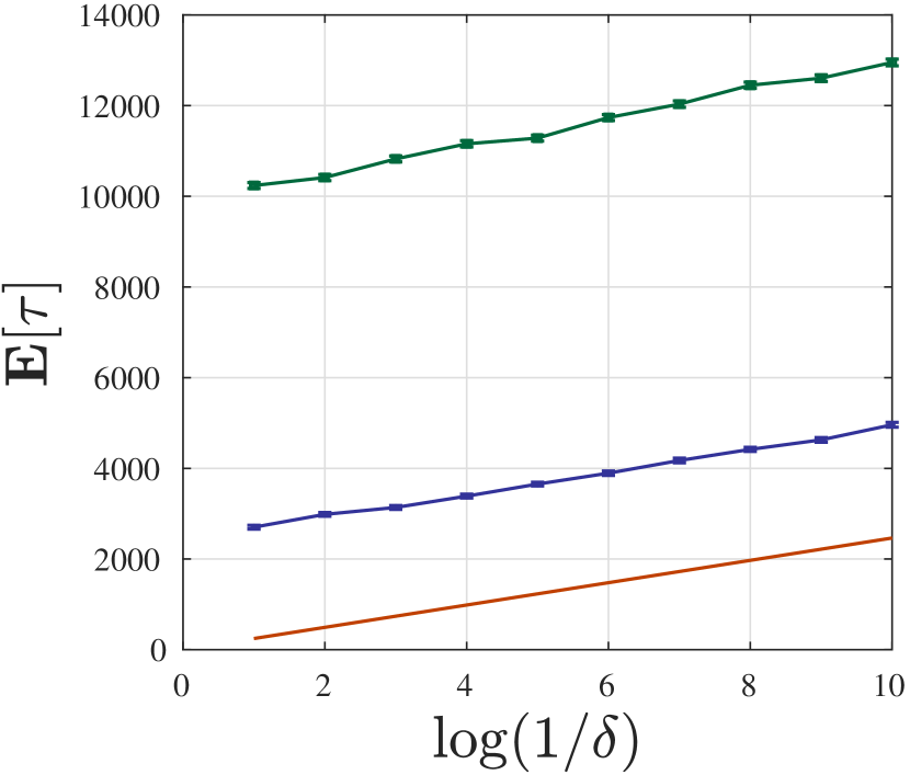
(b) $K=15,p=0.9$.

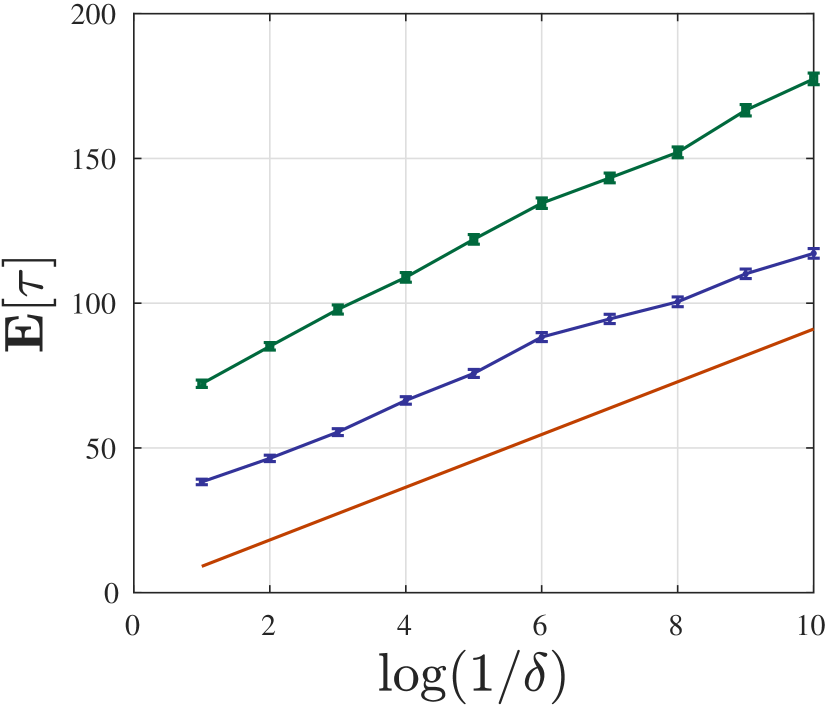
(c) $K=5,p=0.6$.

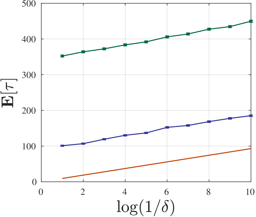
(d) $K=15,p=0.6$.

Figure 2: The empirical averaged stopping times of NE and MTP for different $\delta$ under the worst cases with different $K$ and $p$.

5.1 Fixed-Confidence Setting

First, we consider the worst-case preferences in $\mathcal{M}_{p}^{\mathrm{OA}}$ (as defined in Section 2). Recall that $\mathcal{M}_{p}^{\mathrm{OA}}$ represents the “hardest-to-learn” preferences that minimizes both hardness quantities $I^{N}(\cdot)$ and $I_{\ast}(\cdot)$; see (2) and Proposition 4.2. We conduct our experiments with different target confidence levels $\delta$, as well as values of $K$ and $p$. We plot the empirical averaged stopping times of NE vs. MTP against $\log(1/\delta)$ in each simulation episode. The results are summarized in Figure 2. In addition, we report the empirical means of the CPU runtimes for the whole procedure for $\delta=0.01$ in Table 1.

Table 1: The empirical means of the CPU runtimes (secs) for $\delta=0.01$ under $f^{\mathrm{OA}}$ with different $K$ and $p$.

	$p=0.9$		$p=0.6$
$K$	NE	MTP	NE	MTP
5	0.0773	23.4022	0.0035	0.8957
10	0.1297	108.4158	0.0050	3.5353
15	0.1376	400.5358	0.0064	13.7457

Next, we examine two general (non-worst-case) preferences $f_{1}$ and $f_{2}$, which are calibrated from the Netflix Prize and Debian Logo datasets, respectively using the multinomial logistic (MNL) model. The number of items for preference $f_{1}$ is $4$, while $f_{2}$ has $8$ items. We set $p=0.9$ for both preferences; see Appendix F for detailed information. Figure 3 shows the experimental results under the two general preferences. Note that no explicit lower bound is available for general preferences since $I^{\ast}(f)$ is intractable to solve in general.

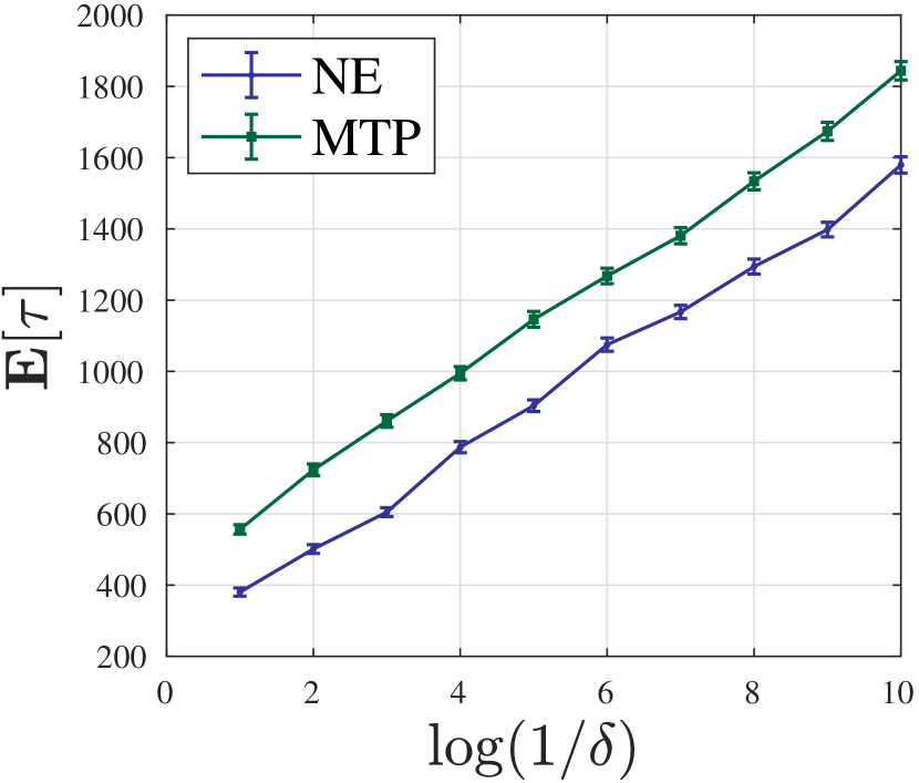
(a) Preference $f_{1}$

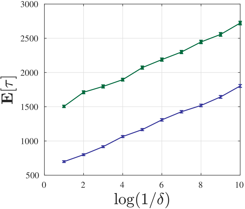
(b) Preference $f_{2}$

Figure 3: The empirical averaged stopping times of NE and MTP for different $\delta$ under two (non-worst-case) preferences $f_{1}$ and $f_{2}$ calibrated from the Netflix Prize and Debian Logo datasets, respectively.

From Figure 2, Table 1 and Figure 3, we have the following observations:

1. Sample Efficiency. Our algorithm NE consistently outperforms its competitor MTP in terms of empirical stopping times across all levels of $\delta$. Notably, in the non-asymptotic regime where $\delta$ is moderately small, NE is significantly superior, indicating its greater practicality in real-world applications.

2. Computational Efficiency. NE is computationally highly efficient and demonstrates a substantial advantage with regard to CPU runtimes as the problem scale increases. It is clear to see that the running speed of NE typically improves upon MTP by three orders of magnitude, especially for large values of $K$.

5.2 Further In-Depth Investigations of NE

Note that based on the hardness quantity ${I^{\mathrm{N}}(\cdot)}$, Proposition 4.3 gives an asymptotic upper bound of the expected stopping time of NE, and the $o_{M}(1)$ term therein vanishes as the exogenous parameter $M$ tends to infinity. The experimental results under the preference $f^{\mathrm{OA}}$ (with $K=10$ and $p=0.9$) and general preference $f_{2}$ are shown in Figure 4. Each sub-figure illustrates the empirical averaged stopping times of NE as well as the asymptotic upper bound with respect to varying input parameters $M$.

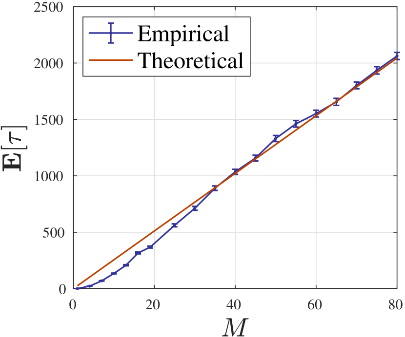
(a) $f^{\mathrm{OA}}$, $K\!=\!10,p\!=\!0.9$.

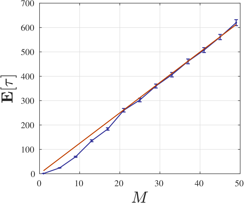
(b) Preference $f_{2}$.

Figure 4: The stopping times of NE for different $M$.

It can be seen from Figure 4 that as $M$ increases, the two curves nearly overlap, supporting the theoretical result in Proposition 4.3. In addition, it confirms the effectiveness of the hardness quantity ${I^{\mathrm{N}}(\cdot)}$ in characterizing the expected stopping time of NE.

6 Conclusions and Future Work

In this paper, we propose and analyze Nested Elimination (or NE), an online algorithm for identifying the best item from choice-based feedback. The algorithm is straightforward in design and implementation, making it a practical solution for various applications. One of the key features of NE is its dynamics and unique elimination criterion. NE can be characterized by a sequence of (biased) random walks on the integer lattice, and the elimination criterion can be represented by a sequence of hitting times of the corresponding random walk. We believe this structure is of independent interest and can be served as a fertile avenue for developing online learning algorithms for other various purposes. Furthermore, our theoretical analysis and numerical experiments clearly demonstrate the computational and sample efficiency of our algorithm.

There are a few opportunities for future work. First, we consider the fixed-confidence formulation of the learning problem. A promising future direction would be to investigate the fixed-budget setting, where the total number of time steps is strictly bounded, by combining the ideas from the multi-armed bandit literature. Second, this paper considers a setting for a fixed separation parameter $p<1$ (or at least when a conservative estimate of $p$ is available). It will be interesting to design an algorithm that is fully agnostic to the value of $p$ as well.

Appendix A An Equivalent Formulation of Nested Elimination

An equivalent formulation of our algorithm NE is presented in Algorithm 2, which only allows eliminating the items one by one, starting with the least voted item, within one time step.

Algorithm 2 Nested Elimination (only allowing eliminating the items one by one)

Input: Tuning parameter $M>0.$

1:  Initialize voting score $W_{0}(i)\leftarrow 0$ for all $i\in[K]$, active item set $S_{\mathrm{active}}\leftarrow[K]$, $t\leftarrow 0$

2:  while $|S_{\mathrm{active}}|>1$ do

3:     Sort the remaining items based on their voting scores. That is, find a ranking $\sigma_{t}:{[|S_{\mathrm{active}}|]}\to S_{\mathrm{active}}$ such that $W_{t}(\sigma_{t}(1))\geq W_{t}(\sigma_{t}(2))\geq\cdots\geq W_{t}(\sigma_{t}(|S_{\mathrm{active}}|))$.

4:     if $\sum_{i=1}^{|S_{\mathrm{active}}|-1}W_{t}(\sigma_{t}(i))-(|S_{\mathrm{active}}|-1)W_{t}(|S_{\mathrm{active}}|)\geq M$ then

5:        $S_{\mathrm{active}}\leftarrow\{\sigma_{t}(1),\ldots,\sigma_{t}(|S_{\mathrm{active}}|-1)\}$

6:     else

7:        Update the timer: $t\leftarrow t+1$.

8:        Display the active set $S_{\mathrm{active}}$, and observe the choice $X_{t}\in S_{\mathrm{active}}$.

9:        Update voting scores based on $X_{t}$:

$$W_{t}(i)\leftarrow\begin{cases}W_{t-1}(i)+1&\text{if }i=X_{t}\\ W_{t-1}(i)&\text{if }i\neq X_{t}.\\ \end{cases}$$

10:     end if

11:  end while

Output: The only element $i_{\mathrm{out}}$ of $S_{\mathrm{active}}$.

Appendix B Proof of Proposition 4.3

For any general preference $f\in\mathcal{M}_{p}$, we define

$$D(f,1):=\frac{1}{1-Kf(K|[K])}$$

and

$$D(f,r):=\frac{(K-r+1)\sum_{i=1}^{r-1}(f(K-r+1|[K-i+1])-f(K-r+2|[K-i+1]))D(f,i)}{1-(K-r+1)f(K-r+1|[K-r+1])}$$

for all $r\in[K-1]\setminus\{1\}$.

Proof of Proposition 4.3.

Before all, note that although Algorithm 1 and Algorithm 2 are equivalent with respect to the final outputs, Algorithm 2 is more convenient for the analysis and thus will be adopted in this proof.

In Algorithm 2, the whole procedure can be divided into $K-1$ stages according to the number of active items. For any stage $r\in[K-1]$, we denote the active item set of size $K-r+1$ as $S_{r}=\{S_{r}^{1},S_{r}^{2},\ldots,S_{r}^{K-r+1}\}$, where the corresponding true ranking satisfies $S_{r}^{1}<S_{r}^{2}<\ldots<S_{r}^{K-r+1}$. In particular, $S_{1}=[K]$. For convenience, we also set $S_{K}$ as the singleton $S_{\mathrm{active}}$ when the algorithm terminates, and refer to the item that is eliminated in stage $r$ as $a_{r}$, i.e., $a_{r}:=S_{r}\setminus S_{r+1}$. Besides, for any stage $r\in[K-1]$, its cumulative time is denoted as $T_{r}$, i.e.,

$$T_{r}:=\inf\left\{t\geq 1\,\middle|\,\sum_{i=1}^{K-r}W_{t}(\sigma_{t}(i))-(K-r)W_{t}(\sigma_{t}(K-r+1))\geq M\right\},$$

which is a stopping time by definition. For ease of notation, we also set $T_{0}=0$. For any stage $r\in[K-1]$, we denote its number of time steps as $\tau_{r}:=T_{r}-T_{r-1}$.

As such, we are interested in bounding the expected stopping time $\operatorname{\mathbb{E}}[\tau]=E[T_{K-1}]$.

Step 1 (Decomposition of the expected stopping time).

For any stage $r\in[K-1]$, we define the event

$$\mathcal{E}_{r}=\{a_{j}=K-j+1\textup{ for all }j\in[r-1]\},$$

which means that our algorithm NE eliminates the worst item correctly in each of the first $r-1$ stages. In particular, $\mathcal{E}_{1}$ is always true and $\mathcal{E}_{1}\supset\mathcal{E}_{2}\supset\cdots\supset\mathcal{E}_{K-1}$. Note that if $\mathcal{E}_{r}$ holds, then the active set $S_{r}$ in stage $r$ must be exactly $[K-r+1]$.

Due to linearity of expectation, we can decompose the expected stopping time as follows:

$$\operatorname{\mathbb{E}}[\tau]=\sum_{r=1}^{K-1}\operatorname{\mathbb{E}}[\tau_{r}]=\sum_{r=1}^{K-1}\operatorname{\mathbb{E}}[\tau_{r}\cdot\mathbbm{1}\{\mathcal{E}_{r}\}]+\sum_{r=1}^{K-1}\operatorname{\mathbb{E}}[\tau_{r}\cdot\mathbbm{1}\{\mathcal{E}_{r}^{c}\}].$$

For convenience, we introduce two shorthand notations

$${\begin{cases}T^{\dagger}=\sum_{r=1}^{K-1}\operatorname{\mathbb{E}}[\tau_{r}\cdot\mathbbm{1}\{\mathcal{E}_{r}\}]\\ T^{\ddagger}=\sum_{r=1}^{K-1}\operatorname{\mathbb{E}}[\tau_{r}\cdot\mathbbm{1}\{\mathcal{E}_{r}^{c}\}].\end{cases}}$$

In the following steps, we will bound $T^{\dagger}$ and $T^{\ddagger}$ separately. Specifically, we will show $T^{\dagger}\leq\frac{\log(1/p)M}{I^{\mathrm{N}}(f)}+o_{M}(1)$ and $T^{\ddagger}=o_{M}(1)$.

Step 2 (Bounding $T^{\dagger}$).

Let us start from the first stage. Notice that the worst item in $S_{1}$ (i.e., item $K$) is not necessarily the one that is going to be eliminated in the first stage, and $\sigma_{T_{1}}$ might not be consistent with the ground truth $\sigma_{*}$. In addition, at time step ${T_{1}}$, $\sum_{i=1}^{K-1}W_{T_{1}}(\sigma_{T_{1}}(i))-(K-1)W_{T_{1}}(\sigma_{T_{1}}(K))$ is exactly equal to $M$ since this quantity of interest can increase by only $1$ within each time step.

Thus, we have

$$\sum_{i=1}^{K-1}W_{T_{1}}(i)-(K-1)W_{T_{1}}(K)\leq\sum_{i=1}^{K-1}W_{T_{1}}(\sigma_{T_{1}}(i))-(K-1)W_{T_{1}}(\sigma_{T_{1}}(K))=M.$$

By taking expectation on both sides, we can get

$$M \geq\operatorname{\mathbb{E}}\left[\sum_{i=1}^{K-1}W_{T_{1}}(i)-(K-1)W_{T_{1}}(K)\right]$$

$$=\left(\sum_{i=1}^{K-1}f(i|[K])-(K-1)f(K|[K])\right)\operatorname{\mathbb{E}}[\tau_{1}]$$

$$=\left({1-Kf(K|[K])}\right)\operatorname{\mathbb{E}}[\tau_{1}\cdot\mathbbm{1}\{\mathcal{E}_{1}\}]$$

$$=\frac{\operatorname{\mathbb{E}}[\tau_{1}\cdot\mathbbm{1}\{\mathcal{E}_{1}\}]}{D(f,1)},$$

where the first equality follows from the optional stopping theorem, and the fact that

$$\sum_{i=1}^{K-1}W_{t}(i)-(K-1)W_{t}(K)-\left(\sum_{i=1}^{K-1}f(i|[K])-(K-1)f(K|[K])\right)t$$

is a martingale in the first stage.

Therefore, it holds that

$${\operatorname{\mathbb{E}}[\tau_{1}\cdot\mathbbm{1}\{\mathcal{E}_{1}\}]}\leq{D(f,1)}M.$$ (10)

For any subsequent stage $r\in[K-1]\setminus\{1\}$, conditioned on any fixed realization of previous stages such that $\mathcal{E}_{r}$ holds,

$$\sum_{i=1}^{K-r}W_{t}\left(i\right)-(K-r)W_{t}\left({K-r+1}\right)-\left(\sum_{i=1}^{K-r}f(i|[K-r+1])-(K-r)f(K-r+1|[K-r+1])\right)t$$

is a martingale for $t\geq T_{r-1}$, and hence we have

$$M \geq\operatorname{\mathbb{E}}\left[\sum_{i=1}^{K-r}W_{T_{r}}\left(i\right)-(K-r)W_{T_{r}}\left({K-r+1}\right)\right]$$

$$=\operatorname{\mathbb{E}}\left[\sum_{i=1}^{K-r}\left(W_{T_{r}}\left(i\right)-W_{T_{r-1}}\left(i\right)\right)-(K-r)\left(W_{T_{r}}\left({K-r+1}\right)-W_{T_{r-1}}\left({K-r+1}\right)\right)\right]$$

$$\phantom{=}+\sum_{i=1}^{K-r}W_{T_{r-1}}\left(i\right)-(K-r)W_{T_{r-1}}\left({K-r+1}\right)$$

$$=\left(\sum_{i=1}^{K-r}f(i|[K-r+1])-(K-r)f(K-r+1|[K-r+1])\right)\operatorname{\mathbb{E}}[\tau_{r}]$$

$$\phantom{=}+M-(K-r+1)(W_{T_{r-1}}({K-r+1})-W_{T_{r-1}}({K-r+2})),$$

where the last equality follows from the fact that item $K-r+2$ is eliminated from the active set $S_{r-1}=[K-r+2]$, i.e.,

$$\sum_{i=1}^{K-r+1}W_{T_{r-1}}\left(i\right)-(K-r+1)W_{T_{r-1}}\left({K-r+2}\right)=M,$$

since $\mathcal{E}_{r}$ occurs.

Therefore, conditioned on any fixed realization of previous stages satisfying $\mathcal{E}_{r}$, we have

$$\operatorname{\mathbb{E}}[\tau_{r}] \leq\frac{(K-r+1)(W_{T_{r-1}}({K-r+1})-W_{T_{r-1}}({K-r+2}))}{\sum_{i=1}^{K-r}f(i|[K-r+1])-(K-r)f(K-r+1|[K-r+1])}$$

$$=\frac{(K-r+1)(W_{T_{r-1}}({K-r+1})-W_{T_{r-1}}({K-r+2}))}{1-(K-r+1)f(K-r+1|[K-r+1])}.$$

By taking expectation with respect to all the realization of previous stages satisfying $\mathcal{E}_{r}$, we can get

$$\operatorname{\mathbb{E}}[\tau_{r}\cdot\mathbbm{1}\{\mathcal{E}_{r}\}] \leq\frac{(K-r+1)\operatorname{\mathbb{E}}[(W_{T_{r-1}}({K-r+1})-W_{T_{r-1}}({K-r+2}))\cdot\mathbbm{1}\{\mathcal{E}_{r}\}]}{1-(K-r+1)f(K-r+1|[K-r+1])}.$$ (11)

Now we consider $\operatorname{\mathbb{E}}[(W_{T_{r-1}}({K-r+1})-W_{T_{r-1}}({K-r+2}))\cdot\mathbbm{1}\{\mathcal{E}_{r}\}]$.

Obviously, it holds that $|W_{T_{r-1}}({K-r+1})-W_{T_{r-1}}({K-r+2})|\leq M$. Otherwise, the algorithm would have already been terminated. Therefore, we can get

$$\phantom{=\ }\operatorname{\mathbb{E}}[(W_{T_{r-1}}({K-r+1})-W_{T_{r-1}}({K-r+2}))\cdot\mathbbm{1}\{\mathcal{E}_{r}\}]$$

$$=\operatorname{\mathbb{E}}[(W_{T_{r-1}}({K-r+1})-W_{T_{r-1}}({K-r+2}))\cdot\mathbbm{1}\{\mathcal{E}_{r-1}\}]$$

$$\phantom{=\ }-\operatorname{\mathbb{E}}[(W_{T_{r-1}}({K-r+1})-W_{T_{r-1}}({K-r+2}))\cdot\mathbbm{1}\{\mathcal{E}_{r-1}\setminus\mathcal{E}_{r}\}]$$

$$\leq\operatorname{\mathbb{E}}[(W_{T_{r-1}}({K-r+1})-W_{T_{r-1}}({K-r+2}))\cdot\mathbbm{1}\{\mathcal{E}_{r-1}\}]+M\mathbb{P}(\mathcal{E}_{r-1}\setminus\mathcal{E}_{r}).$$ (12)

In stage $r-1$, supposing that $\mathcal{E}_{r-1}$ occurs, the active set $S_{r-1}$ is $[K-r+2]$ and

$$(W_{t}({K-r+1})-W_{t}({K-r+2}))-(f(K-r+1|[K-r+2])-f(K-r+2|[K-r+2]))t$$

is a martingale for $t\geq T_{r-2}$.

Therefore, by the optional stopping theorem, we can obtain

$$\phantom{=\ }\operatorname{\mathbb{E}}[(W_{T_{r-1}}({K-r+1})-W_{T_{r-1}}({K-r+2}))\cdot\mathbbm{1}\{\mathcal{E}_{r-1}\}]$$

$$=(f(K-r+1|[K-r+2])-f(K-r+2|[K-r+2]))\operatorname{\mathbb{E}}[\tau_{r-1}\cdot\mathbbm{1}\{\mathcal{E}_{r-1}\}]$$

$$\phantom{=\ }+\operatorname{\mathbb{E}}[(W_{T_{r-2}}({K-r+1})-W_{T_{r-2}}({K-r+2}))\cdot\mathbbm{1}\{\mathcal{E}_{r-1}\}].$$ (13)

Combining (12) and (13) gives

$$\phantom{=\ }\operatorname{\mathbb{E}}[(W_{T_{r-1}}({K-r+1})-W_{T_{r-1}}({K-r+2}))\cdot\mathbbm{1}\{\mathcal{E}_{r}\}]$$

$$\leq(f(K-r+1|[K-r+2])-f(K-r+2|[K-r+2]))\operatorname{\mathbb{E}}[\tau_{r-1}\cdot\mathbbm{1}\{\mathcal{E}_{r-1}\}]$$

$$\phantom{=\ }+\operatorname{\mathbb{E}}[(W_{T_{r-2}}({K-r+1})-W_{T_{r-2}}({K-r+2}))\cdot\mathbbm{1}\{\mathcal{E}_{r-1}\}]+M\mathbb{P}(\mathcal{E}_{r-1}\setminus\mathcal{E}_{r}).$$

Observe that the above analysis of $\operatorname{\mathbb{E}}[(W_{T_{r-1}}({K-r+1})-W_{T_{r-1}}({K-r+2}))\cdot\mathbbm{1}\{\mathcal{E}_{r}\}]$ can also be applied to $\operatorname{\mathbb{E}}[(W_{T_{i}}({K-r+1})-W_{T_{i}}({K-r+2}))\cdot\mathbbm{1}\{\mathcal{E}_{i+1}\}]$ for all $i\in[r-1]$. Thus, we have

$$\phantom{=\ }\operatorname{\mathbb{E}}[(W_{T_{r-1}}({K-r+1})-W_{T_{r-1}}({K-r+2}))\cdot\mathbbm{1}\{\mathcal{E}_{r}\}]$$

$$\leq\sum_{i=1}^{r-1}(f(K-r+1|[K-i+1])-f(K-r+2|[K-i+1]))\operatorname{\mathbb{E}}[\tau_{i}\cdot\mathbbm{1}\{\mathcal{E}_{i}\}]$$

$$\phantom{=\ }+\operatorname{\mathbb{E}}[(W_{T_{0}}({K-r+1})-W_{T_{0}}({K-r+2}))\cdot\mathbbm{1}\{\mathcal{E}_{1}\}]+M\sum_{i=1}^{r-1}\mathbb{P}(\mathcal{E}_{i}\setminus\mathcal{E}_{i+1})$$

$$=\sum_{i=1}^{r-1}(f(K-r+1|[K-i+1])-f(K-r+2|[K-i+1]))\operatorname{\mathbb{E}}[\tau_{i}\cdot\mathbbm{1}\{\mathcal{E}_{i}\}]+M\sum_{i=1}^{r-1}\mathbb{P}(\mathcal{E}_{i}\setminus\mathcal{E}_{i+1})$$

Together with (11) and Lemma B.1, it holds that

$$\operatorname{\mathbb{E}}[\tau_{r}\cdot\mathbbm{1}\{\mathcal{E}_{r}\}] \leq\frac{(K-r+1)\sum_{i=1}^{r-1}(f(K-r+1|[K-i+1])-f(K-r+2|[K-i+1]))\operatorname{\mathbb{E}}[\tau_{i}\cdot\mathbbm{1}\{\mathcal{E}_{i}\}]}{1-(K-r+1)f(K-r+1|[K-r+1])}$$

$$\phantom{=}+\frac{(K-r+1)M\sum_{i=2}^{r}Q_{*}^{i}}{1-(K-r+1)f(K-r+1|[K-r+1])}$$ (14)

for all subsequent stage $r\in[K-1]\setminus\{1\}$.

To reduce clutter and ease the reading, we define

$$\hat{D}(f,1):=D(f,1)=\frac{1}{1-Kf(K|[K])}$$

and

$$\hat{D}(f,r) :=\frac{(K-r+1)\sum_{i=1}^{r-1}(f(K-r+1|[K-i+1])-f(K-r+2|[K-i+1]))\hat{D}(f,i)}{1-(K-r+1)f(K-r+1|[K-r+1])}$$

$$\phantom{:=}+\frac{(K-r+1)\sum_{i=2}^{r}Q_{*}^{i}}{1-(K-r+1)f(K-r+1|[K-r+1])}$$

for all $r\in[K-1]\setminus\{1\}$. Moreover, it is straightforward to verify that

$$\left(\hat{D}(f,r)-D(f,r)\right)M=o_{M}(1)$$

based on the definition of $Q_{*}^{i}$ for $i=[r]\setminus\{1\}$ in Lemma B.1.

Accordingly, Inequalities (10) and (14) jointly imply that for all $r\in[K-1]$,

$$\operatorname{\mathbb{E}}[\tau_{r}\cdot\mathbbm{1}\{\mathcal{E}_{r}\}]\leq\hat{D}(f,r)M,$$

which further leads to

$$T^{\dagger} =\sum_{r=1}^{K-1}\operatorname{\mathbb{E}}[\tau_{r}\cdot\mathbbm{1}\{\mathcal{E}_{r}\}]$$

$$\leq\sum_{r=1}^{K-1}\hat{D}(f,r)M$$

$$=\sum_{r=1}^{K-1}D(f,r)M+\sum_{r=1}^{K-1}\left(\hat{D}(f,r)-D(f,r)\right)M$$

$$=\frac{\log(1/p)M}{I^{\mathrm{N}}(f)}+\sum_{r=2}^{K-1}\left(\hat{D}(f,r)-D(f,r)\right)M$$

as desired.

Step 3 (Bounding $T^{\ddagger}$).

Note that $\operatorname{\mathbb{E}}[\tau_{1}\cdot\mathbbm{1}\{\mathcal{E}_{1}^{c}\}]=0$. Thus, we consider $\operatorname{\mathbb{E}}[\tau_{r}\cdot\mathbbm{1}\{\mathcal{E}_{r}^{c}\}]$ for arbitrary $r\in[K-1]\setminus\{1\}$ in the following.

Conditioned on any fixed realization of previous stages such that $\mathcal{E}_{r}$ does not occur,

$$\sum_{i=1}^{K-r}W_{t}\left(S_{r}^{i}\right)-(K-r)W_{t}\left(S_{r}^{K-r+1}\right)-\left(\sum_{i=1}^{K-r}f(S_{r}^{i}|S_{r})-(K-r)f(S_{r}^{K-r+1}|S_{r})\right)t$$

is a martingale for $t\geq T_{r-1}$, and hence we have

$$M \geq\operatorname{\mathbb{E}}\left[\sum_{i=1}^{K-r}W_{T_{r}}\left(S_{r}^{i}\right)-(K-r)W_{T_{r}}\left(S_{r}^{K-r+1}\right)\right]$$

$$=\operatorname{\mathbb{E}}\left[\sum_{i=1}^{K-r}\left(W_{T_{r}}\left(S_{r}^{i}\right)-W_{T_{r-1}}\left(S_{r}^{i}\right)\right)-(K-r)\left(W_{T_{r}}\left(S_{r}^{K-r+1}\right)-W_{T_{r-1}}\left(S_{r}^{K-r+1}\right)\right)\right]$$

$$\phantom{=}+\sum_{i=1}^{K-r}W_{T_{r-1}}\left(S_{r}^{i}\right)-(K-r)W_{T_{r-1}}\left(S_{r}^{K-r+1}\right)$$

$$=\left(\sum_{i=1}^{K-r}f(S_{r}^{i}|S_{r})-(K-r)f(S_{r}^{K-r+1}|S_{r})\right)\operatorname{\mathbb{E}}[\tau_{r}]+\sum_{i=1}^{K-r}W_{T_{r-1}}\left(S_{r}^{i}\right)-(K-r)W_{T_{r-1}}\left(S_{r}^{K-r+1}\right).$$ (15)

For all $i\in[K-r]$, it holds that

$$W_{T_{r-1}}\left(S_{r}^{i}\right)-W_{T_{r-1}}\left(S_{r}^{K-r+1}\right)\geq-M.$$

Otherwise, the algorithm would have already been terminated. Thus, we have

$$\sum_{i=1}^{K-r}W_{T_{r-1}}\left(S_{r}^{i}\right)-(K-r)W_{T_{r-1}}\left(S_{r}^{K-r+1}\right)\geq-(K-r)M.$$

In addition, due to the definition of $\mathcal{M}_{p}$, we have

$$\sum_{i=1}^{K-r}f(S_{r}^{i}|S_{r})-(K-r)f(S_{r}^{K-r+1}|S_{r}) =1-(K-r+1)f(S_{r}^{K-r+1}|S_{r})$$

$$\geq 1-\frac{(K-r+1)(1-p)p^{K-r}}{1-p^{K-r+1}}$$

$$=\frac{(K-r)p^{K-r+1}-(K-r+1)p^{K-r}+1}{1-p^{K-r+1}}.$$

Together with (15), we have

$$\operatorname{\mathbb{E}}[\tau_{r}] \leq\frac{(K-r+1)({1-p^{K-r+1}})M}{(K-r)p^{K-r+1}-(K-r+1)p^{K-r}+1},$$

which is conditioned on any fixed realization of previous stages satisfying $\mathcal{E}_{r}^{c}$.

By taking expectation with respect to all the realization of previous stages satisfying $\mathcal{E}_{r}^{c}$, we can get

$$\operatorname{\mathbb{E}}[\tau_{r}\cdot\mathbbm{1}\{\mathcal{E}_{r}^{c}\}] \leq\frac{(K-r+1)({1-p^{K-r+1}})M}{(K-r)p^{K-r+1}-(K-r+1)p^{K-r}+1}\mathbb{P}(\mathcal{E}_{r}^{c}).$$ (16)

Since $\mathcal{E}_{r}^{c}=\bigcup_{i=1}^{r-1}\left(\mathcal{E}_{i}\setminus\mathcal{E}_{i+1}\right)$ and $\mathcal{E}_{i}\setminus\mathcal{E}_{i+1}$ for $i\in[r-1]$ are pairwise mutually exclusive events, along with Lemma B.1,

$$\mathbb{P}(\mathcal{E}_{r}^{c})=\sum_{i=1}^{r-1}\mathbb{P}(\mathcal{E}_{i}\setminus\mathcal{E}_{i+1})\leq\sum_{i=2}^{r}Q_{*}^{i}.$$ (17)

Finally, by combining (16) and (17), we can bound $T^{\ddagger}$ as

$$T^{\ddagger} =\sum_{r=2}^{K-1}\operatorname{\mathbb{E}}[\tau_{r}\cdot\mathbbm{1}\{\mathcal{E}_{r}^{c}\}]$$

$$\leq\sum_{r=2}^{K-1}\sum_{i=2}^{r}\frac{(K-r+1)({1-p^{K-r+1}})MQ_{*}^{i}}{(K-r)p^{K-r+1}-(K-r+1)p^{K-r}+1}.$$

Notice that $T^{\ddagger}=o_{M}(1)$, as a result of the definition of $Q_{*}^{i}$ for $i=[r]\setminus\{1\}$ in Lemma B.1.

Therefore, the proof of Proposition 4.3 is completed, and we have

$$\operatorname{\mathbb{E}}[\tau]\leq\frac{\log(1/p)M}{I^{\mathrm{N}}(f)}+\underbrace{\sum_{r=2}^{K-1}\left(\hat{D}(f,r)-D(f,r)\right)M+\sum_{r=2}^{K-1}\sum_{i=2}^{r}\frac{(K-r+1)({1-p^{K-r+1}})MQ_{*}^{i}}{(K-r)p^{K-r+1}-(K-r+1)p^{K-r}+1}}_{o_{M}(1)}.$$ (18)

∎

Lemma B.1.

For any customer preference $f\in\mathcal{M}_{p}$ and any stage $r\in[K-1]\setminus\{1\}$,

$$\mathbb{P}(\mathcal{E}_{r-1}\setminus\mathcal{E}_{r})\leq Q_{*}^{r}:=\sum_{i=1}^{K-r+1}\left({q_{*}^{r,i}}\right)^{M}$$

where $q_{*}^{r,i}\in(0,1)$ is defined in (23) in the corresponding proof and does not depend on $M$.

Proof of Lemma B.1.

Recall that the item that is eliminated in stage $r-1$ is denoted as $a_{r-1}$. Therefore, we can decompose the probability of interest as follows:

$$\mathbb{P}(\mathcal{E}_{r-1}\setminus\mathcal{E}_{r}) =\mathbb{P}(\mathcal{E}_{r-1}\wedge a_{r-1}\neq K-r+2)$$

$$=\sum_{i=1}^{K-r+1}\mathbb{P}(\mathcal{E}_{r-1}\wedge a_{r-1}=i).$$

Next, for any $i\in[K-r+1]$, we will analyze $\mathbb{P}(\mathcal{E}_{r-1}\wedge a_{r-1}=i)$, which is the probability that our algorithm NE eliminates the worst item correctly in each of the first $r-2$ stages and eliminates item $i$ in stage $r-1$.

Step 1.

At certain time step $t$ in any stage $\bar{r}\in[r-1]$, suppose that $\mathcal{E}_{\bar{r}}$ holds, which ensures that the current active set is $[K-\bar{r}+1]$. Consider

$$Y^{r,i}_{t}(\alpha):=\sum_{j=1}^{K-r+2}W_{t}(j)-(K-r+2)W_{t}(i)+\alpha(W_{t}(K-r+2)-W_{t}(i))$$

with some $\alpha>0$ to be carefully selected soon. We claim that as long as

$$\operatorname{\mathbb{E}}[Y^{r,i}_{t+1}(\alpha)\mid Y^{r,i}_{t}(\alpha)]<Y^{r,i}_{t}(\alpha),$$ (19)

then there exists $0<q<1$ such that $\left(1/q\right)^{Y^{r,i}_{t}(\alpha)}$ is a supermartingale, i.e.,

$$\operatorname{\mathbb{E}}\left[\left(\frac{1}{q}\right)^{Y^{r,i}_{t+1}(\alpha)}\,\middle|\,\left(\frac{1}{q}\right)^{Y^{r,i}_{t}(\alpha)}\right]\leq\left(\frac{1}{q}\right)^{Y^{r,i}_{t}(\alpha)}.$$ (20)

In fact, the condition in (19) is equivalent to

$$\sum_{j=1}^{K-r+2}f(j|[K-\bar{r}+1])-(K-r+2)f(i|[K-\bar{r}+1])+\alpha(f(K-r+2|[K-\bar{r}+1])\\ -f(i|[K-\bar{r}+1]))<0$$ (21)

which is trivially true for large enough $\alpha$, since $f(K-r+2|[K-\bar{r}+1])-f(i|[K-\bar{r}+1])<0$.

On the other hand, (20) requires

$$\frac{1}{q}\left(\sum_{j=1}^{K-r+1}f(j|[K-\bar{r}+1])-f(i|[K-\bar{r}+1])\right)+q^{K-r+1+\alpha}\cdot f(i|[K-\bar{r}+1])$$

$$+\frac{1}{q^{1+\alpha}}\cdot f(K-r+2|[K-\bar{r}+1])+(1-f([K-r+2]|[K-\bar{r}+1]))\leq 1.$$ (22)

Let

$$g\left(q\right) :=\frac{1}{q}\left(\sum_{j=1}^{K-r+1}f(j|[K-\bar{r}+1])-f(i|[K-\bar{r}+1])\right)+q^{K-r+1+\alpha}\cdot f(i|[K-\bar{r}+1])$$

$$\phantom{:=}+\frac{1}{q^{1+\alpha}}\cdot f(K-r+2|[K-\bar{r}+1])+(1-f([K-r+2]|[K-\bar{r}+1])).$$

Since $g(1)=1$ and

$$\phantom{=\ }g^{\prime}(1)$$

$$=-\left(\sum_{j=1}^{K-r+1}f(j|[K-\bar{r}+1])-f(i|[K-\bar{r}+1])\right)+({K-r+1+\alpha})\cdot f(i|[K-\bar{r}+1])$$

$$\phantom{=}-({1+\alpha})\cdot f(K-r+2|[K-\bar{r}+1])$$

$$=-\left(\sum_{j=1}^{K-r+2}f(j|[K-\bar{r}+1])-(K-r+2)f(i|[K-\bar{r}+1])+\alpha(f(K-r+2|[K-\bar{r}+1])-f(i|[K-\bar{r}+1]))\right)$$

$$>0,$$

there exists $0<q<1$ such that (22) holds. So the claim that we made above is correct.

Step 2.

Now we choose $q_{*}^{r,i}$ as

$$q_{*}^{r,i}=\min_{\alpha>0}~{}~{}q$$ (23)

$$\phantom{q_{*}^{r,i}=}~{}\text{ s.t. }\text{\eqref{equation_condition4} and \eqref{equation_condition3} hold for all }\bar{r}\in[r-1]$$

$$\phantom{q_{*}^{r,i}=~{}\text{ s.t. }}0<q<1.$$

We also refer to the corresponding optimal solution of decision variable $\alpha$ as $\alpha_{*}^{r,i}$. Notice that both $q_{*}^{r,i}$ and $\alpha_{*}^{r,i}$ do not depend on $M$.

With such choices of $q_{*}^{r,i}$ and $\alpha_{*}^{r,i}$, for any stage $\bar{r}\in[r-1]$, given that $\mathcal{E}_{\bar{r}}$ occurs, $\left(\frac{1}{q_{*}^{r,i}}\right)^{Y^{r,i}_{t}(\alpha_{*}^{r,i})}$ is a supermartingale until the end of the current stage.

Step 3.

Following the above result, we can sequentially apply the optional stopping theorem in the first $r-1$ stages. Since ${Y^{r,i}_{T_{0}}(\alpha_{*}^{r,i})}=0$, we have

$$1 =\operatorname{\mathbb{E}}\left[\left(\frac{1}{q_{*}^{r,i}}\right)^{Y^{r,i}_{T_{0}}(\alpha_{*}^{r,i})}\right]\geq\operatorname{\mathbb{E}}\left[\left(\frac{1}{q_{*}^{r,i}}\right)^{Y^{r,i}_{T_{1}}(\alpha_{*}^{r,i})}\right]$$

$$=\operatorname{\mathbb{E}}\left[\left(\frac{1}{q_{*}^{r,i}}\right)^{Y^{r,i}_{T_{1}}(\alpha_{*}^{r,i})}\cdot\mathbbm{1}\left\{\mathcal{E}_{1}\right\}\right]\geq\operatorname{\mathbb{E}}\left[\left(\frac{1}{q_{*}^{r,i}}\right)^{Y^{r,i}_{T_{1}}(\alpha_{*}^{r,i})}\cdot\mathbbm{1}\left\{\mathcal{E}_{2}\right\}\right]$$

$$\geq\operatorname{\mathbb{E}}\left[\left(\frac{1}{q_{*}^{r,i}}\right)^{Y^{r,i}_{T_{2}}(\alpha_{*}^{r,i})}\cdot\mathbbm{1}\left\{\mathcal{E}_{2}\right\}\right]\geq\operatorname{\mathbb{E}}\left[\left(\frac{1}{q_{*}^{r,i}}\right)^{Y^{r,i}_{T_{2}}(\alpha_{*}^{r,i})}\cdot\mathbbm{1}\left\{\mathcal{E}_{3}\right\}\right]$$

$$\geq\cdots$$

$$\geq\operatorname{\mathbb{E}}\left[\left(\frac{1}{q_{*}^{r,i}}\right)^{Y^{r,i}_{T_{r-2}}(\alpha_{*}^{r,i})}\cdot\mathbbm{1}\left\{\mathcal{E}_{r-2}\right\}\right]\geq\operatorname{\mathbb{E}}\left[\left(\frac{1}{q_{*}^{r,i}}\right)^{Y^{r,i}_{T_{r-2}}(\alpha_{*}^{r,i})}\cdot\mathbbm{1}\left\{\mathcal{E}_{r-1}\right\}\right]$$

$$\geq\operatorname{\mathbb{E}}\left[\left(\frac{1}{q_{*}^{r,i}}\right)^{Y^{r,i}_{T_{r-1}}(\alpha_{*}^{r,i})}\cdot\mathbbm{1}\left\{\mathcal{E}_{r-1}\right\}\right]$$

where we also utilize the fact that $\mathcal{E}_{1}\supset\mathcal{E}_{2}\supset\cdots\supset\mathcal{E}_{K-1}$ and the nonnegativity of $\left(\frac{1}{q_{*}^{r,i}}\right)^{Y^{r,i}_{t}(\alpha_{*}^{r,i})}$.

Note that $\mathcal{E}_{r-1}$ implies $S_{r-1}=[K-r+2]$. Furthermore, if $a_{r-1}=i$, then it must be the case that $W_{T_{r-1}}(i)\leq W_{T_{r-1}}(K-r+2)$ and $\sum_{j=1}^{K-r+2}W_{T_{r-1}}(j)-(K-r+2)W_{T_{r-1}}(i)=M$, which gives ${Y^{r,i}_{T_{r-1}}(\alpha_{*}^{r,i})}>M$ since $\alpha_{*}^{r,i}>0$.

Hence, we can get

$$1 \geq\operatorname{\mathbb{E}}\left[\left(\frac{1}{q_{*}^{r,i}}\right)^{Y^{r,i}_{T_{r-1}}(\alpha_{*}^{r,i})}\cdot\mathbbm{1}\left\{\mathcal{E}_{r-1}\right\}\right]$$

$$\geq\operatorname{\mathbb{E}}\left[\left(\frac{1}{q_{*}^{r,i}}\right)^{Y^{r,i}_{T_{r-1}}(\alpha_{*}^{r,i})}\cdot\mathbbm{1}\left\{\mathcal{E}_{r-1}\wedge a_{r-1}=i\right\}\right]$$

$$\geq\mathbb{P}(\mathcal{E}_{r-1}\wedge a_{r-1}=i)\cdot\left(\frac{1}{q_{*}^{r,i}}\right)^{M}$$

which is equivalent to

$$\mathbb{P}(\mathcal{E}_{r-1}\wedge a_{r-1}=i)\leq\left({q_{*}^{r,i}}\right)^{M}.$$

Therefore, the proof of Lemma B.1 is completed now. ∎

Appendix C Proof of Proposition 4.2

We will prove Proposition 4.2 in a slightly different flow than how it is described.

First, we demonstrate in Lemma C.1 that the class $\mathcal{M}_{p}^{\mathrm{OA}}$ minimizes $\{I^{\mathrm{N}}(f):{f\in\mathcal{M}_{p}}\}$. Next, in Lemma C.2, we prove that for any preference $f\in\mathcal{M}_{p}^{\mathrm{OA}}$, $I^{\mathrm{N}}(f)=I_{*}^{\mathrm{OA}}$. Finally, Proposition 4.2 follows directly from Lemma C.1 and Lemma C.2.

Lemma C.1.

It holds that

$$\mathcal{M}_{p}^{\mathrm{OA}}\subset\operatorname*{arg\,min}_{f\in\mathcal{M}_{p}}{I^{\mathrm{N}}(f)}.$$

Lemma C.2.

For any preference $f\in\mathcal{M}_{p}^{\mathrm{OA}}$, it holds that

$$I^{\mathrm{N}}(f)={I_{*}^{\mathrm{OA}}}.$$

Remark C.3.

As a matter of fact, in light of the proof of Lemma C.1, we can have a more accurate characterization of the minimizer in Proposition 4.2. Specifically, the minimum of $\{I^{\mathrm{N}}(f):{f\in\mathcal{M}_{p}}\}$ is attained if and only if

$$f(j|[r])=\frac{1-p}{1-p^{r}}p^{j-1}$$

for all $r\in[K]$ and $j\in[r]$.

C.1 Proof of Lemma C.1

Proof of Lemma C.1.

We will prove the desired result in the following steps.

Step 1.

Recall that for any general preference $f\in\mathcal{M}_{p}$,

$$D(f,1)=\frac{1}{1-Kf(K|[K])}$$

and

$$D(f,r)=\frac{(K-r+1)\sum_{i=1}^{r-1}(f(K-r+1|[K-i+1])-f(K-r+2|[K-i+1]))D(f,i)}{1-(K-r+1)f(K-r+1|[K-r+1])}$$ (24)

for all $r\in[K-1]\setminus\{1\}$.

In the following, we will prove via induction that for all $r\in[K-1]\setminus\{1\}$, it holds that

$$\sum_{i=1}^{r-1}(f([K-r+1]|[K-i+1])-(K-r+1)f(K-r+2|[K-i+1]))D(f,i)=1$$ (25)

We only need to consider $K\geq 3$ as the case that $K=2$ is vacuous. For $r=2$, the claim of (25) is equivalent to

$$(f([K-1]|[K])-(K-1)f(K|[K]))D(f,1)=1,$$

which holds trivially due to the definition of $D(f,1)$.

Now suppose that (25) is true for $r=\bar{r}$ with $2\leq\bar{r}\leq K-2$. Then we can derive

$$\phantom{=\ }\sum_{i=1}^{\bar{r}}(f([K-\bar{r}]|[K-i+1])-(K-\bar{r})f(K-\bar{r}+1|[K-i+1]))D(f,i)-1$$

$$=\sum_{i=1}^{\bar{r}}(f([K-\bar{r}]|[K-i+1])-(K-\bar{r})f(K-\bar{r}+1|[K-i+1]))D(f,i)$$

$$\phantom{=\ }-\sum_{i=1}^{\bar{r}-1}(f([K-\bar{r}+1]|[K-i+1])-(K-\bar{r}+1)f(K-\bar{r}+2|[K-i+1]))D(f,i)$$

$$=\sum_{i=1}^{\bar{r}-1}(K-\bar{r}+1)(f(K-\bar{r}+2|[K-i+1]))-f(K-\bar{r}+1|[K-i+1])))D(f,i)$$

$$\phantom{=\ }+(f([K-\bar{r}]|[K-\bar{r}+1])-(K-\bar{r})f(K-\bar{r}+1|[K-\bar{r}+1]))D(f,\bar{r})$$

$$=\sum_{i=1}^{\bar{r}-1}(K-\bar{r}+1)(f(K-\bar{r}+2|[K-i+1]))-f(K-\bar{r}+1|[K-i+1])))D(f,i)$$

$$\phantom{=\ }+(1-(K-\bar{r}+1)f(K-\bar{r}+1|[K-\bar{r}+1]))D(f,\bar{r})$$

$$=0,$$

where the last equality results from the definition of $D(f,\bar{r})$ as (24).

Therefore, (25) is also true for $r=\bar{r}+1$ and the induction step is completed.

By mathematical induction, we can conclude that our claim (25) holds for all $r\in[K-1]\setminus\{1\}$.

Next, combining (24) and (25) results in another helpful expression of $D(f,r)$, i.e.,

$$D(f,r)=\frac{1-\sum_{i=1}^{r-1}\left(f([K-r]|[K-i+1])-(K-r)f(K-r+1|[K-i+1])\right)D(f,i)}{1-(K-r+1)f(K-r+1|[K-r+1])},$$ (26)

for all $r\in[K-1]\setminus\{1\}$.

Step 2.

For any general preference $f\in\mathcal{M}_{p}$, due to the definition of $D(f,1)$ and Lemma C.4, we have

$$D(f,1) =\frac{1}{1-Kf(K|[K])}$$

$$=\frac{1}{f([K-1]|[K])-(K-1)f(K|[K])}$$

$$\leq\frac{1-p^{K}}{(K-1)p^{K}-Kp^{K-1}+1},$$

which further gives

$$\frac{(1-p)p^{K-1}}{1-p^{K}}D(f,1)\leq\frac{(1-p)p^{K-1}}{(K-1)p^{K}-Kp^{K-1}+1}.$$ (27)

For any $r\in[K-1]\setminus\{1\}$, again by Lemma C.4, we can get

$$f([K-r]|[K-i+1])-(K-r)f(K-r+1|[K-i+1])\geq\frac{(K-r)p^{K-r+1}-(K-r+1)p^{K-r}+1}{1-p^{K-i+1}}$$

for any $i\in[r-1]$, and

$${1-(K-r+1)f(K-r+1|[K-r+1])}\geq\frac{({K-r})p^{K-r+1}-{(K-r+1)}p^{{K-r}}+1}{1-p^{K-r+1}}.$$

Plug the above two inequalities into the expression of $D(f,r)$ in (26), then we have

$$D(f,r)+\sum_{i=1}^{r-1}\frac{1-p^{K-r+1}}{1-p^{K-i+1}}D(f,i)\leq\frac{1-p^{K-r+1}}{({K-r})p^{K-r+1}-{(K-r+1)}p^{{K-r}}+1}.$$ (28)

By multiplying (28) with different coefficients for all $r\in[K-1]\setminus\{1\}$, we can get

$$\frac{(1-p)p^{K-r}}{1-p^{K-r+1}}D(f,r)+\sum_{i=1}^{r-1}\frac{(1-p)p^{K-r}}{1-p^{K-i+1}}D(f,i)\leq\frac{(1-p)p^{K-r}}{({K-r})p^{K-r+1}-{(K-r+1)}p^{{K-r}}+1}$$ (29)

for all $r\in[K-2]\setminus\{1\}$, and

$$D(f,K-1)+\sum_{i=1}^{K-2}\frac{1-p^{2}}{1-p^{K-i+1}}D(f,i)\leq\frac{1+p}{1-p}.$$ (30)

Step 3.

Finally, adding up Inequalities (27), (29) and (30) leads to

$$\phantom{\leq{}}\sum_{r=1}^{K-2}\frac{(1-p)p^{K-r}}{1-p^{K-r+1}}D(f,r)+\sum_{r=2}^{K-2}\sum_{i=1}^{r-1}\frac{(1-p)p^{K-r}}{1-p^{K-i+1}}D(f,i)+D(f,K-1)+\sum_{i=1}^{K-2}\frac{1-p^{2}}{1-p^{K-i+1}}D(f,i)$$

$$\leq\frac{(1-p)p^{K-1}}{(K-1)p^{K}-Kp^{K-1}+1}+\sum_{r=2}^{K-2}\frac{(1-p)p^{K-r}}{({K-r})p^{K-r+1}-{(K-r+1)}p^{{K-r}}+1}+\frac{1+p}{1-p}$$

$$\Longleftrightarrow \phantom{\leq{}}\sum_{r=1}^{K-2}\frac{(1-p)p^{K-r}}{1-p^{K-r+1}}D(f,r)+\sum_{r=1}^{K-3}\sum_{i=r+1}^{K-2}\frac{(1-p)p^{K-i}}{1-p^{K-r+1}}D(f,r)+\sum_{r=1}^{K-2}\frac{1-p^{2}}{1-p^{K-r+1}}D(f,r)+D(f,K-1)$$

$$\leq\sum_{r=1}^{K-2}\frac{(1-p)p^{K-r}}{({K-r})p^{K-r+1}-{(K-r+1)}p^{{K-r}}+1}+\frac{1+p}{1-p}$$

$$\Longleftrightarrow \phantom{\leq{}}\sum_{r=1}^{K-2}\frac{p^{K-r}-p^{K-r+1}}{1-p^{K-r+1}}D(f,r)+\sum_{r=1}^{K-3}\frac{p^{2}-p^{K-r}}{1-p^{K-r+1}}D(f,r)+\sum_{r=1}^{K-2}\frac{1-p^{2}}{1-p^{K-r+1}}D(f,r)+D(f,K-1)$$

$$\leq\sum_{r=1}^{K-2}\frac{(1-p)p^{K-r}}{({K-r})p^{K-r+1}-{(K-r+1)}p^{{K-r}}+1}+\frac{1+p}{1-p}$$

$$\Longleftrightarrow \phantom{\leq{}}\sum_{r=1}^{K-1}D(f,r)\leq\sum_{r=1}^{K-2}\frac{(1-p)p^{K-r}}{({K-r})p^{K-r+1}-{(K-r+1)}p^{{K-r}}+1}+\frac{1+p}{1-p}.$$

Therefore, we obtain that for any general preference $f\in\mathcal{M}_{p}$,

$$\frac{\log(1/p)}{I^{\mathrm{N}}(f)}=\sum_{r=1}^{K-1}D(f,r)\leq\sum_{r=1}^{K-2}\frac{(1-p)p^{K-r}}{({K-r})p^{K-r+1}-{(K-r+1)}p^{{K-r}}+1}+\frac{1+p}{1-p}.$$ (31)

Note that the above upper bound of $\frac{\log(1/p)}{I^{\mathrm{N}}(f)}$ does not depend on the particular choice of $f$. Furthermore, in view of Lemma C.4, exact equality in (31) can be achieved if $f\in\mathcal{M}_{p}^{\mathrm{OA}}$.

As a result, we conclude that

$$\mathcal{M}_{p}^{\mathrm{OA}}\subset\operatorname*{arg\,min}_{f\in\mathcal{M}_{p}}{I^{\mathrm{N}}(f)}.$$

as desired.

∎

Lemma C.4.

For any $r\in[K]$ and $i\in[r-1]$,

$$\min_{f\in\mathcal{M}_{p}}f([i]|[r])-if(i+1|[r])=\frac{ip^{i+1}-(i+1)p^{i}+1}{1-p^{r}}.$$ (32)

Furthermore, the minimum is attained if and only if

$$f(j|[r])=\frac{1-p}{1-p^{r}}p^{j-1}$$

for all $j\in[r]$.

Proof of Lemma C.4.

Notice that only the preference on $[r]$ (i.e., $f(j|[r])$ for $j\in[r]$) matters in terms of the minimization problem (32). For ease of notation, we denote $x_{j}:=f(j|[r])$ for all $j\in[r]$. Then the problem (32) of interest can be reformulated as the following optimization problem:

$$\min_{x}\,\sum_{j=1}^{i}x_{j}-ix_{i+1}$$

$$\text{ s.t. }\,px_{j}-x_{j+1}\geq 0,\,\forall j\in[r-1]$$

$$\phantom{\text{ s.t. }}\,\sum_{j=1}^{r}x_{j}=1$$

$$\phantom{\text{ s.t. }}\,x_{j}\geq 0,\,\forall j\in[r].$$

We let $h(x):=\sum_{j=1}^{i}x_{j}-ix_{i+1}$. Due to the constraints on $x$, for all $1\leq j_{1}<j_{2}\leq r-1$, it holds that

$$x_{j_{1}}\geq p^{j_{1}-j_{2}}x_{j_{2}},$$ (33)

where the exact equality is achieved if and only if $px_{j}=x_{j+1}$ for all $j_{1}\leq j<j_{2}$.

Therefore, by (33), we can get

$$\sum_{j=1}^{i}x_{j}\geq\left(\sum_{j=1}^{i}p^{-j}\right)x_{i+1},$$

which is equivalent to

$$-ix_{i+1}\geq\frac{-ip^{i}(1-p)}{1-p^{i}}\sum_{j=1}^{i}x_{j}.$$

Then we can bound $h(x)$ as follows:

$$h(x) \geq\sum_{j=1}^{i}x_{j}-\frac{ip^{i}(1-p)}{1-p^{i}}\sum_{j=1}^{i}x_{j}$$

$$=\frac{ip^{i+1}-(i+1)p^{i}+1}{1-p^{i}}\sum_{j=1}^{i}x_{j}.$$ (34)

For any $j\in[i]$, again by (33), we have

$$x_{j} =\frac{1-p^{i}}{1-p^{r}}x_{j}+\frac{p^{i}-p^{r}}{1-p^{r}}x_{j}$$

$$\geq\frac{1-p^{i}}{1-p^{r}}x_{j}+\frac{p^{i}-p^{r}}{1-p^{r}}\cdot\frac{1}{\sum_{j^{\prime}=i+1}^{r}p^{j^{\prime}-j}}\sum_{j^{\prime}=i+1}^{r}x_{j^{\prime}}$$

$$=\frac{1-p^{i}}{1-p^{r}}x_{j}+\frac{p^{j-1}(1-p)}{1-p^{r}}\sum_{j^{\prime}=i+1}^{r}x_{j^{\prime}}.$$ (35)

Adding up (35) for all $j\in[i]$ results in

$$\sum_{j=1}^{i}x_{j} \geq\sum_{j=1}^{i}\left(\frac{1-p^{i}}{1-p^{r}}x_{j}+\frac{p^{j-1}(1-p)}{1-p^{r}}\sum_{j^{\prime}=i+1}^{r}x_{j^{\prime}}\right)$$

$$=\frac{1-p^{i}}{1-p^{r}}\sum_{j=1}^{i}x_{j}+\sum_{j^{\prime}=i+1}^{r}x_{j^{\prime}}\sum_{j=1}^{i}\frac{p^{j-1}(1-p)}{1-p^{r}}$$

$$=\frac{1-p^{i}}{1-p^{r}}\sum_{j=1}^{i}x_{j}+\frac{1-p^{i}}{1-p^{r}}\sum_{j^{\prime}=i+1}^{r}x_{j^{\prime}}$$

$$=\frac{1-p^{i}}{1-p^{r}}\sum_{j=1}^{r}x_{j}.$$

Together with (34), we conclude that

$$h(x)\geq\frac{ip^{i+1}-(i+1)p^{i}+1}{1-p^{r}}.$$ (36)

It is straightforward to check the lower bound in (36) can be binding if and only if

$$x_{j}=\frac{1-p}{1-p^{r}}p^{j-1}$$

for all $j\in[r]$.

Thus, the proof of Lemma C.4 is finished.

∎

C.2 Proof of Lemma C.2

Proof of Lemma C.2.

It suffices to show for any preference $f\in\mathcal{M}_{p}^{\mathrm{OA}}$,

$$\frac{\log(1/p)}{I^{\mathrm{N}}(f)}=\frac{\log(1/p)}{I_{*}^{\mathrm{OA}}},$$ (37)

where

$${I_{*}^{\mathrm{OA}}}=(1-p)\log\left(\frac{1}{p}\right)\left(1+\sum_{j=2}^{K}\frac{p^{j-1}}{1+2p+\cdots+(j-1)p^{j-2}}\right)^{-1}$$

as shown in Feng et al. (2021).

In fact, according to (31) in the proof of Proposition 4.2, we have

$$\frac{\log(1/p)}{I^{\mathrm{N}}(f)}=\sum_{r=1}^{K-2}\frac{(1-p)p^{K-r}}{({K-r})p^{K-r+1}-{(K-r+1)}p^{{K-r}}+1}+\frac{1+p}{1-p}$$

for any preference $f\in\mathcal{M}_{p}^{\mathrm{OA}}$.

For the right-hand side of (37), by the combinatorial identity

$$1+2p+\cdots+(j-1)p^{j-2}=\frac{(j-1)p^{j}-jp^{j-1}+1}{(1-p)^{2}},$$

it holds that

$$\frac{\log(1/p)}{I_{*}^{\mathrm{OA}}} =\frac{1}{1-p}\left(1+\sum_{j=2}^{K}\frac{p^{j-1}}{1+2p+\cdots+(j-1)p^{j-2}}\right)$$

$$=\frac{1}{1-p}\left(1+\sum_{j=2}^{K}\frac{(1-p)^{2}p^{j-1}}{(j-1)p^{j}-jp^{j-1}+1}\right)$$

$$=\frac{1}{1-p}+\frac{(1-p)p}{p^{2}-2p+1}+\sum_{j=3}^{K}\frac{(1-p)p^{j-1}}{(j-1)p^{j}-jp^{j-1}+1}$$

$$=\frac{1+p}{1-p}+\sum_{r=1}^{K-2}\frac{(1-p)p^{K-r}}{(K-r)p^{K-r+1}-(K-r+1)p^{K-r}+1}$$

$$=\frac{\log(1/p)}{I^{\mathrm{N}}(f)}$$

which leads to the desired result of (37).

Therefore, Lemma C.2 is proved. ∎

Appendix D Proof of Proposition 4.4

Proof of Proposition 4.4.

Here we also adopt the notations introduced in the proof of Proposition 4.3.

Recall that for any stage $r\in[K-1]$, the active set of size $K-r+1$ is referred to as $S_{r}$. Therefore, we are interested in bounding

$$\mathbb{P}(i_{\mathrm{out}}\neq 1) =\mathbb{P}(1\not\in S_{K})$$

$$=\sum_{r=1}^{K-1}\mathbb{P}(1\not\in S_{r+1}\wedge 1\in S_{r}).$$ (38)

In the following, we will analyze $\mathbb{P}(1\not\in S_{r+1}\wedge 1\in S_{r})$, which represents the probability of eliminating the best item in the given item set $[K]$ (i.e., item $1$) in stage $r$.

Step 1.

For any stage $r\in[K-1]$, condition on any fixed realization of previous stages such that the best item is not eliminated prior to stage $r$, i.e., $1\in S_{r}$.

Then we claim that for this fixed realization of $S_{r}=\{S_{r}^{1},S_{r}^{2},\ldots,S_{r}^{K-r+1}\}$ with $S_{r}^{1}=1$,

$${\left(\frac{1}{p}\right)}^{\sum_{i=2}^{K-r+1}W_{t}(S_{r}^{i})-(K-r)W_{t}(S_{r}^{1})}$$

is a supermartingale for $t\geq T_{r-1}$.

To verify this favorable property, it suffices to show

$$\frac{1}{p}\sum_{i=2}^{K-r+1}f(S_{r}^{i}|S_{r})+p^{K-r}f(S_{r}^{1}|S_{r})\leq 1.$$

Actually, the above inequality is equivalent to

$$f(S_{r}^{1}|S_{r})\geq\frac{1-p}{1-p^{K-r+1}},$$

which holds trivially due to the definition of $\mathcal{M}_{p}$.

Therefore, by the optional stopping theorem, it holds that

$$\phantom{\geq\ }{\left(\frac{1}{p}\right)}^{\sum_{i=2}^{K-r+1}W_{T_{r-1}}(S_{r}^{i})-(K-r)W_{T_{r-1}}(S_{r}^{1})}$$

$$\geq\operatorname{\mathbb{E}}\left[{\left(\frac{1}{p}\right)}^{\sum_{i=2}^{K-r+1}W_{T_{r}}(S_{r}^{i})-(K-r)W_{T_{r}}(S_{r}^{1})}\right]$$

$$\geq\mathbb{P}(1\not\in S_{r+1})\cdot{\left(\frac{1}{p}\right)}^{M}$$

where the last inequality follows from the fact that if $1\in S_{r}$ but $1\not\in S_{r+1}$, then

$${\sum_{i=2}^{K-r+1}W_{T_{r}}(S_{r}^{i})-(K-r)W_{T_{r}}(S_{r}^{1})}=M.$$

Again by taking expectation with respect to all the realization of previous stages satisfying $1\in S_{r}$, we can derive

$$\mathbb{P}(1\not\in S_{r+1}\wedge 1\in S_{r})\leq\operatorname{\mathbb{E}}\left[{\left(\frac{1}{p}\right)}^{\sum_{i=2}^{K-r+1}W_{T_{r-1}}(S_{r}^{i})-(K-r)W_{T_{r-1}}(S_{r}^{1})}\cdot\mathbbm{1}\{1\in S_{r}\}\right]\cdot p^{M}.$$ (39)

Step 2.

Consider any stage $r\in[K-1]$.

For ease of presentation, we define $\hat{S}_{r}:=S_{r}\setminus\{S_{r}^{1}\}=\{S_{r}^{2},S_{r}^{3},\ldots,S_{r}^{K-r+1}\}$. Notice that $\hat{S}_{r}$ is also a random variable. In addition, we use lower-case $\hat{s}_{r}$ and $\{s_{r}^{i}\}_{i=2}^{K-r+1}$ to denote the indicators of the specific realizations of $\hat{S}_{r}$ and $\{S_{r}^{i}\}_{i=2}^{K-r+1}$, respectively.

Then we have

$$\phantom{\geq\ }\operatorname{\mathbb{E}}\left[{\left(\frac{1}{p}\right)}^{\sum_{i=2}^{K-r+1}W_{T_{r-1}}(S_{r}^{i})-(K-r)W_{T_{r-1}}(S_{r}^{1})}\cdot\mathbbm{1}\{1\in S_{r}\}\right]$$

$$=\sum_{\hat{s}_{r}\subset[K]\setminus\{1\}}\operatorname{\mathbb{E}}\left[{\left(\frac{1}{p}\right)}^{\sum_{i=2}^{K-r+1}W_{T_{r-1}}(s_{r}^{i})-(K-r)W_{T_{r-1}}(1)}\cdot\mathbbm{1}\left\{\{1\}\cup\hat{s}_{r}=S_{r}\right\}\right]$$

$$=\sum_{\hat{s}_{r}\subset[K]\setminus\{1\}}\operatorname{\mathbb{E}}\left[{\left(\frac{1}{p}\right)}^{\sum_{i=2}^{K-r+1}W_{T_{r-1}}(s_{r}^{i})-(K-r)W_{T_{r-1}}(1)}\cdot\mathbbm{1}\left\{\{1\}\cup\hat{s}_{r}\subset S_{r}\right\}\right].$$ (40)

Next, for any ${\hat{s}_{r}\subset[K]\setminus\{1\}}$, we will show via mathematical induction that

$$\operatorname{\mathbb{E}}\left[{\left(\frac{1}{p}\right)}^{\sum_{i=2}^{K-r+1}W_{T_{r-1}}(s_{r}^{i})-(K-r)W_{T_{r-1}}(1)}\cdot\mathbbm{1}\left\{\{1\}\cup\hat{s}_{r}\subset S_{r}\right\}\right]\leq 1.$$ (41)

Consider the first stage, where the active set $S_{1}$ is $[K]$. Since

$${\left(\frac{1}{p}\right)}^{\sum_{i=2}^{K-r+1}W_{t}(s_{r}^{i})-(K-r)W_{t}(1)}$$

is a supermartingale in the first phase, by the optional stopping theorem, it holds that

$$1 =\operatorname{\mathbb{E}}\left[{\left(\frac{1}{p}\right)}^{\sum_{i=2}^{K-r+1}W_{T_{0}}(s_{r}^{i})-(K-r)W_{T_{0}}(1)}\right]$$

$$\geq\operatorname{\mathbb{E}}\left[{\left(\frac{1}{p}\right)}^{\sum_{i=2}^{K-r+1}W_{T_{1}}(s_{r}^{i})-(K-r)W_{T_{1}}(1)}\right]$$

$$\geq\operatorname{\mathbb{E}}\left[{\left(\frac{1}{p}\right)}^{\sum_{i=2}^{K-r+1}W_{T_{1}}(s_{r}^{i})-(K-r)W_{T_{1}}(1)}\cdot\mathbbm{1}\left\{\{1\}\cup\hat{s}_{r}\subset S_{2}\right\}\right].$$

Suppose that for all $j$ in $\{2,3,\dots,\bar{r}-1\}$,

$$\operatorname{\mathbb{E}}\left[{\left(\frac{1}{p}\right)}^{\sum_{i=2}^{K-r+1}W_{T_{j-1}}(s_{r}^{i})-(K-r)W_{T_{j-1}}(1)}\cdot\mathbbm{1}\left\{\{1\}\cup\hat{s}_{r}\subset S_{j}\right\}\right]\leq 1$$

is correct. Then consider the ${\bar{r}}$-th stage. Since for any fixed realization of $S_{\bar{r}}$ such that $\{1\}\cup\hat{s}_{r}\subset S_{\bar{r}}$,

$${\left(\frac{1}{p}\right)}^{\sum_{i=2}^{K-r+1}W_{t}(s_{r}^{i})-(K-r)W_{t}(1)}$$

is a supermartingale for $t\geq T_{{\bar{r}}-1}$, again by the optional stopping theorem, it holds that

$$1 \geq\operatorname{\mathbb{E}}\left[{\left(\frac{1}{p}\right)}^{\sum_{i=2}^{K-r+1}W_{T_{{\bar{r}}-1}}(s_{r}^{i})-(K-r)W_{T_{{\bar{r}}-1}}(1)}\cdot\mathbbm{1}\left\{\{1\}\cup\hat{s}_{r}\subset S_{\bar{r}}\right\}\right]$$

$$\geq\operatorname{\mathbb{E}}\left[{\left(\frac{1}{p}\right)}^{\sum_{i=2}^{K-r+1}W_{T_{{\bar{r}}}}(s_{r}^{i})-(K-r)W_{T_{{\bar{r}}}}(1)}\cdot\mathbbm{1}\left\{\{1\}\cup\hat{s}_{r}\subset S_{\bar{r}}\right\}\right]$$

$$\geq\operatorname{\mathbb{E}}\left[{\left(\frac{1}{p}\right)}^{\sum_{i=2}^{K-r+1}W_{T_{{\bar{r}}}}(s_{r}^{i})-(K-r)W_{T_{{\bar{r}}}}(1)}\cdot\mathbbm{1}\left\{\{1\}\cup\hat{s}_{r}\subset S_{\bar{r}+1}\right\}\right]$$

which establishes the induction step and further proves (41).

Note that the cardinality of $\hat{s}_{r}$ is $K-r$. Therefore, combining (40) and (41) gives

$$\operatorname{\mathbb{E}}\left[{\left(\frac{1}{p}\right)}^{\sum_{i=2}^{K-r+1}W_{T_{r-1}}(S_{r}^{i})-(K-r)W_{T_{r-1}}(S_{r}^{1})}\cdot\mathbbm{1}\{1\in S_{r}\}\right]\leq\binom{K-1}{K-r}.$$

Together with (39), we can get

$$\mathbb{P}(1\not\in S_{r+1}\wedge 1\in S_{r})\leq\binom{K-1}{K-r}p^{M}.$$ (42)

Step 3.

Finally, by plugging (42) into (38), we have

$$\mathbb{P}(i_{\mathrm{out}}\neq 1) =\sum_{r=1}^{K-1}\mathbb{P}(1\not\in S_{r+1}\wedge 1\in S_{r})$$

$$\leq\sum_{r=1}^{K-1}\binom{K-1}{K-r}p^{M}$$

$$=(2^{K-1}-1)p^{M}$$

which completes the proof of Proposition 4.4.

∎

Appendix E Proof of Theorem 4.1

Proof of Theorem 4.1.

Consider any fixed confidence level $\delta\in(0,1)$. On account of Proposition 4.4, with parameter $M=\frac{\log(1/\delta)+\log(\beta(K))}{\log(1/p)}$, NE outputs an item $i_{\mathrm{out}}$ satisfying

$$\mathbb{P}(i_{\mathrm{out}}\neq 1)\leq\beta(K)\cdot p^{M}=\delta$$

for any customer preference $f\in\mathcal{M}_{p}$.

Therefore, according to Definition 2.4, to confirm our algorithm NE is $\delta$-PAC, it remains to show $\mathbb{P}(\tau<\infty)=1$. Note that for any random variable, finite expectation implies almost sure finiteness. So by Proposition 4.3, we can get that the stopping time $\tau$ is finite almost surely, which concludes that NE is $\delta$-PAC.

Furthermore, based on Proposition 4.3 as well as Equation (18) in the corresponding proof, the expected stopping time ${\operatorname{\mathbb{E}}[\tau]}$ can be upper bounded as follows:

$$\operatorname{\mathbb{E}}[\tau] \leq\frac{\log(1/p)M}{I^{\mathrm{N}}(f)}+\sum_{r=2}^{K-1}\left(\hat{D}(f,r)-D(f,r)\right)M+\sum_{r=2}^{K-1}\sum_{i=2}^{r}\frac{(K-r+1)({1-p^{K-r+1}})MQ_{*}^{i}}{(K-r)p^{K-r+1}-(K-r+1)p^{K-r}+1}$$

$$=\frac{\log(1/\delta)}{I^{\mathrm{N}}(f)}+\frac{\log(\beta(K))}{I^{\mathrm{N}}(f)}$$

$$\phantom{=}+\sum_{r=2}^{K-1}\left(\hat{D}(f,r)-D(f,r)\right)M+\sum_{r=2}^{K-1}\sum_{i=2}^{r}\frac{(K-r+1)({1-p^{K-r+1}})MQ_{*}^{i}}{(K-r)p^{K-r+1}-(K-r+1)p^{K-r}+1}.$$

Here, recall that $\{Q_{*}^{i}\}$ is defined in Lemma B.1.

Finally, with $M=\frac{\log(1/\delta)+\log(\beta(K))}{\log(1/p)}$, we have

$$\hat{C}_{f}(\delta):=\sum_{r=2}^{K-1}\left(\hat{D}(f,r)-D(f,r)\right)M+\sum_{r=2}^{K-1}\sum_{i=2}^{r}\frac{(K-r+1)({1-p^{K-r+1}})MQ_{*}^{i}}{(K-r)p^{K-r+1}-(K-r+1)p^{K-r}+1}=o_{M}(1)=o_{\frac{1}{\delta}}(1).$$

Therefore, the theorem holds by letting

$$C_{f}:=\frac{\log(\beta(K))}{I^{\mathrm{N}}(f)}+\sup_{\delta\in(0,1)}\hat{C}_{f}(\delta)<+\infty.$$ (43)

∎

Appendix F Additional Implementation Details and Numerical Results

F.1 Additional Implementation Details of MTP

Initialization.

At the initial time step, i.e., $t=1$, we randomly assign a ranking on the item set $[K]$ as the estimated global ranking, and use this ranking to determine the first display set. In fact, through extensive tests, we notice that the initialization step has minimal influence on the overall performance.

Stopping Rule.

For the threshold function used in the stopping rule of MTP, we follow the one indicated in the experimental parts of Feng et al. (2021), i.e.,

$$\log((K-1)(K-1)!)+\log(1/\delta).$$

Optimization Solver.

As we noted in Section 4.1, both the display rule and the stopping rule of MTP require solving some combinatorial optimization problems. Throughout the experiments, we follow the exact integer linear programming formulation in Feng et al. (2021), and utilize Gurobi 9.5.2 as the optimization solver.

F.2 Fixed-Confidence Setting

Worst-Case Preferences.

The empirical averaged stopping times of NE and MTP for different confidence levels $\delta$ under the worst cases with $K=15$ and different $p$ are shown in Figure 5.

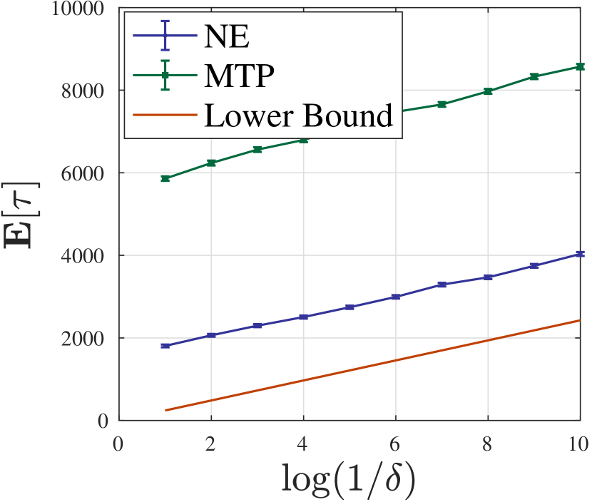
(a) $p=0.9$.

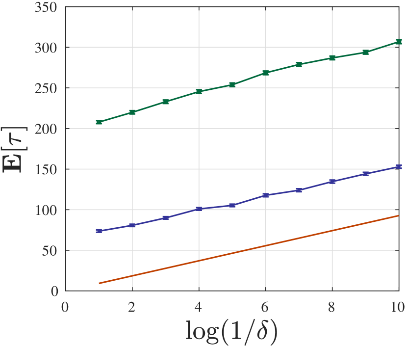
(b) $p=0.6$.

Figure 5: The empirical averaged stopping times of NE and MTP for different $\delta$ under the worst cases with $K=10$ and different $p$.

General Preferences.

Both the Netflix Prize and Debian Logo datasets are provided by PrefLib (Mattei & Walsh, 2013). The Netflix Prize dataset Bennett et al. (2007) consists of $823$ preference rankings over $4$ movies, while the Debian Logo dataset consists of $143$ preference rankings over $8$ candidates for the Debian logo. To generate one general (not worst-case) preference from each raw dataset, we consider each preference ranking as an interaction between the company and the customers, and hence the top-ranked item is treated as the choice of the customer. Next, we fit an MNL model (defined in Definition F.1), using maximum likelihood estimation. Finally, note that both final outputs, $f_{1}$ and $f_{2}$, belong to $\mathcal{M}_{p}$ with $p=0.9$.

Definition F.1 (Luce (1959)).

Under the multinomial logistic (MNL) model, a preference $f$ is characterized by a non-negative vector of attraction scores $\{\nu_{1},\nu_{2},\ldots,\nu_{K}\}$, and the probability that item $i$ is chosen from the display set $S\in\mathcal{S}$ is

$$f(i|S)=\frac{\nu_{i}}{\sum_{j\in S}\nu_{j}}.$$

F.3 In-Depth Investigations of NE

The empirical averaged and theoretical stopping times of NE for different input parameters $M$ under the worst cases and general cases are shown in Figure 6 and Figure 7, respectively.

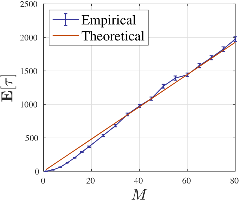
(a) $K=5,p=0.9$.

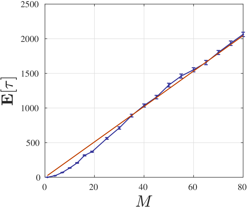
(b) $K=10,p=0.9$.

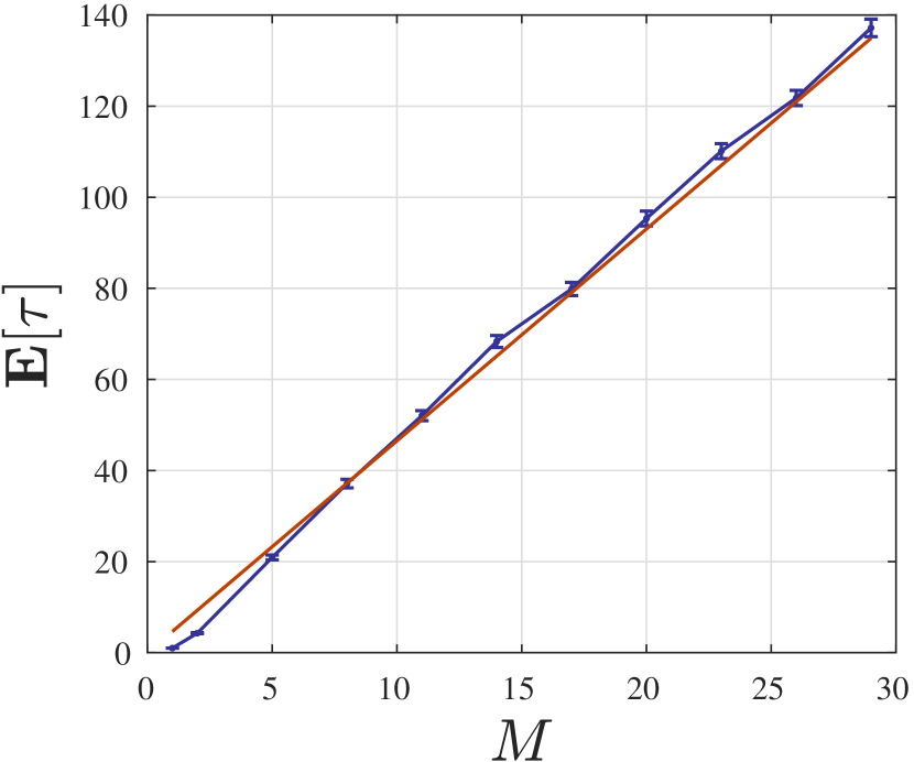
(c) $K=5,p=0.6$.

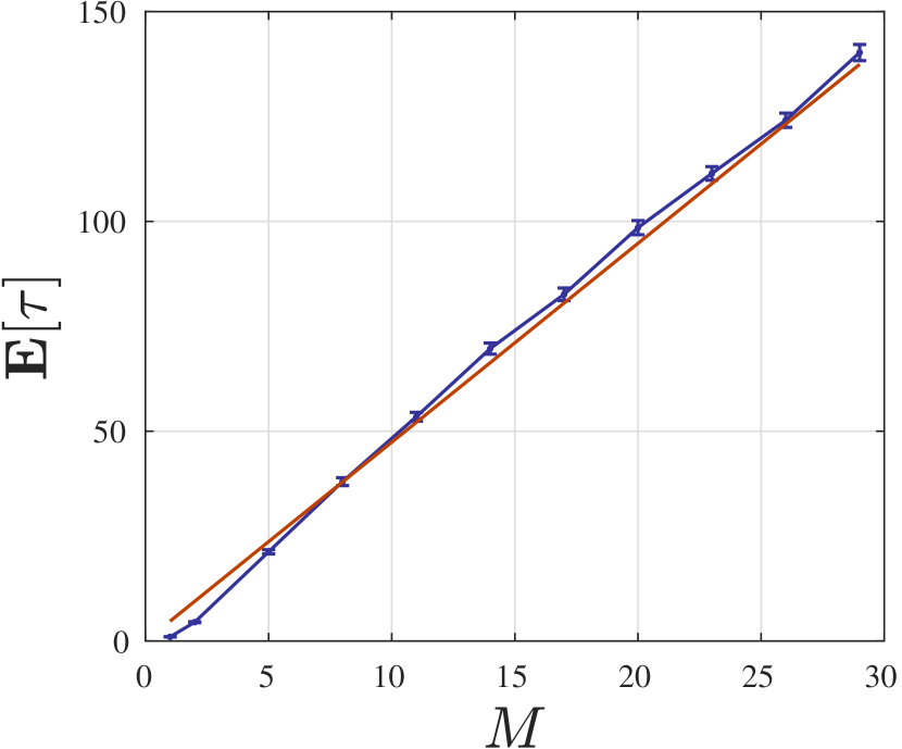
(d) $K=10,p=0.6$.

Figure 6: The stopping times of NE for different $M$ under the worst cases with different $K$ and $p$.

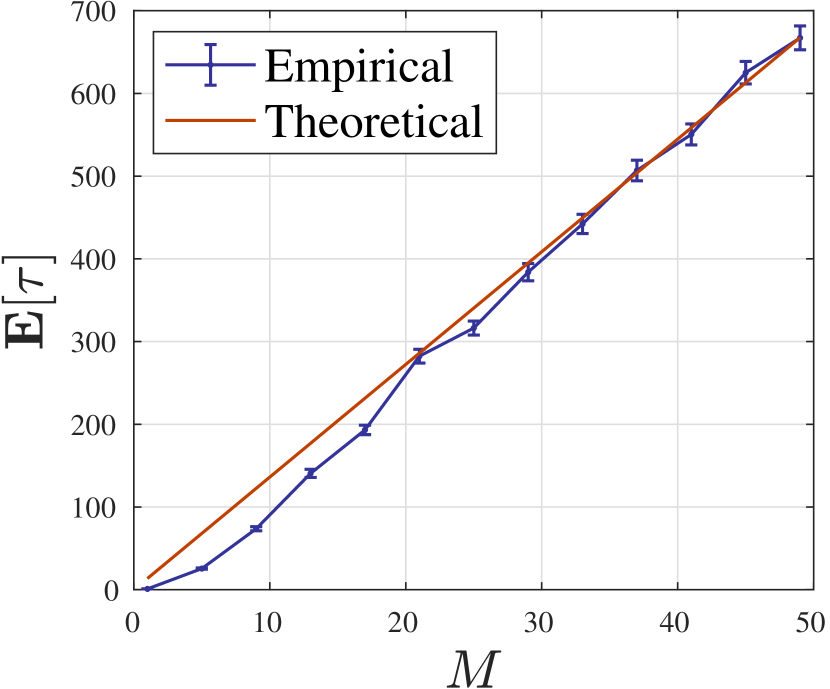
(a) Preference $f_{1}$.

(b) Preference $f_{2}$.

Figure 7: The stopping times of NE for different $M$ under two general preferences $f_{1}$ and $f_{2}$.

References

• Agrawal & Goyal (2012) Agrawal, S. and Goyal, N. Analysis of Thompson sampling for the multi-armed bandit problem. In Conference on Learning Theory (COLT), pp.  39–1. JMLR Workshop and Conference Proceedings, 2012.
• Audibert et al. (2010) Audibert, J.-Y., Bubeck, S., and Munos, R. Best arm identification in multi-armed bandits. In Conference on Learning Theory (COLT), pp.  41–53, 2010.
• Auer et al. (2002) Auer, P., Cesa-Bianchi, N., and Fischer, P. Finite-time analysis of the multiarmed bandit problem. Machine Learning, 47(2):235–256, 2002.
• Bennett et al. (2007) Bennett, J., Lanning, S., et al. The netflix prize. In Proceedings of KDD cup and workshop, volume 2007, pp.  35, 2007.
• Braverman & Mossel (2008) Braverman, M. and Mossel, E. Noisy sorting without resampling. In Proceedings of the nineteenth annual ACM-SIAM symposium on Discrete algorithms, pp.  268–276, 2008.
• Bubeck & Cesa-Bianchi (2012) Bubeck, S. and Cesa-Bianchi, N. Regret analysis of stochastic and nonstochastic multi-armed bandit problems. Foundations and Trends® in Machine Learning, 5(1):1–122, 2012.
• Chen et al. (2018) Chen, X., Li, Y., and Mao, J. A nearly instance optimal algorithm for top-k ranking under the multinomial logit model. In Proceedings of the Twenty-Ninth Annual ACM-SIAM Symposium on Discrete Algorithms, pp.  2504–2522. SIAM, 2018.
• Chernoff (1959) Chernoff, H. Sequential design of experiments. The Annals of Mathematical Statistics, 30(3):755–770, 1959.
• Even-Dar et al. (2006) Even-Dar, E., Mannor, S., Mansour, Y., and Mahadevan, S. Action elimination and stopping conditions for the multi-armed bandit and reinforcement learning problems. Journal of Machine Learning Research, 7(6), 2006.
• Feng & Tang (2022) Feng, Y. and Tang, Y. On a mallows-type model for (ranked) choices. In Advances in Neural Information Processing Systems, 2022.
• Feng et al. (2021) Feng, Y., Caldentey, R., and Ryan, C. T. Robust learning of consumer preferences. Operations Research, 2021.
• Garivier & Kaufmann (2016) Garivier, A. and Kaufmann, E. Optimal best arm identification with fixed confidence. In Conference on Learning Theory, pp.  998–1027. PMLR, 2016.
• Kalyanakrishnan & Stone (2010) Kalyanakrishnan, S. and Stone, P. Efficient selection of multiple bandit arms: Theory and practice. In ICML, 2010.
• Karnin et al. (2013) Karnin, Z., Koren, T., and Somekh, O. Almost optimal exploration in multi-armed bandits. In International Conference on Machine Learning, pp. 1238–1246. PMLR, 2013.
• Kaufmann et al. (2016) Kaufmann, E., Cappé, O., and Garivier, A. On the complexity of best-arm identification in multi-armed bandit models. Journal of Machine Learning Research, 17(1):1–42, 2016.
• Lattimore & Szepesvári (2020) Lattimore, T. and Szepesvári, C. Bandit Algorithms. Cambridge University Press, 2020.
• Luce (1959) Luce, R. Individual Choice Behavior: A Theoretical Analysis. Wiley, 1959.
• Mattei & Walsh (2013) Mattei, N. and Walsh, T. Preflib: A library of preference data http://preflib.org. In Proceedings of the 3rd International Conference on Algorithmic Decision Theory (ADT 2013), Lecture Notes in Artificial Intelligence. Springer, 2013.
• Saha & Gopalan (2020) Saha, A. and Gopalan, A. Best-item learning in random utility models with subset choices. In International Conference on Artificial Intelligence and Statistics, pp.  4281–4291. PMLR, 2020.
• Shalev-Shwartz et al. (2012) Shalev-Shwartz, S. et al. Online learning and online convex optimization. Foundations and Trends® in Machine Learning, 4(2):107–194, 2012.
• Thompson (1933) Thompson, W. R. On the likelihood that one unknown probability exceeds another in view of the evidence of two samples. Biometrika, 25(3-4):285–294, 1933.
• Wauthier et al. (2013) Wauthier, F., Jordan, M., and Jojic, N. Efficient ranking from pairwise comparisons. In International Conference on Machine Learning, pp. 109–117. PMLR, 2013.