Two-layer Space-oriented Partitioning for Non-point Data

Abstract

Non-point spatial objects (e.g., polygons, linestrings, etc.) are ubiquitous. We study the problem of indexing non-point objects in memory for range queries and spatial intersection joins. We propose a secondary partitioning technique for space-oriented partitioning indices (e.g., grids), which improves their performance significantly, by avoiding the generation and elimination of duplicate results. Our approach is easy to implement and can be used by any space-partitioning index to significantly reduce the cost of range queries and intersection joins. In addition, the secondary partitions can be processed independently, which makes our method appropriate for distributed and parallel indexing. Experiments on real datasets confirm the advantage of our approach against alternative duplicate elimination techniques and data-oriented state-of-the-art spatial indices. We also show that our partitioning technique, paired with optimized partition-to-partition join algorithms, typically reduces the cost of spatial joins by around 50%.

1 Introduction

Spatial data management has been extensively studied, especially for disk-resident data [1]. Nowadays, in most applications, collections of points or minimum bounding rectangles (MBRs) of extended objects can easily fit in the memory of even a commodity machine. Although a number of scalable systems for spatial data have been developed in the past decade [2, 3, 4, 5, 6], the problem of in-memory management of large-scale spatial data has received relatively little attention.

In this paper, we study the problem of indexing MBRs of non-point spatial objects (e.g., polygons, linestrings, etc.) in memory, for the efficient evaluation of the filter step of range queries and spatial intersection joins. Large volumes of non-point data are ubiquitous, hence, their effective management is always timely. Besides Geographic Information Systems, domains that manage big volumes of such data include graphics (e.g., management of huge meshes [7]), neuroscience (e.g., building and indexing a spatial model of the brain [8]), and location-based analytics (e.g., managing spatial influence regions of mobile users in order to facilitate effective POI recommendations [9]).

Motivation. Spatial access methods can be divided into two categories; space-oriented partitioning (SOP) and data-oriented partitioning (DOP) approaches. Indices of the first category divide the space into spatially disjoint partitions. As a result, objects that overlap with multiple partitions must be replicated (or clipped) in each of them. DOP methods allow the extents of the partitions to overlap and ensure that their contents are disjoint (i.e., each object is assigned to exactly one partition). For disk-resident data, DOP approaches (such as the R-tree [10] and its variants) are considered to be the best, because they avoid data replication and they have a balanced structure. However, SOP approaches (especially grids) are gaining ground due to their efficiency in search and updates in main memory [11, 12, 13, 14, 15, 16]. In addition, query evaluation over grids is embarassingly parallelizable and SOP is widely used in distributed spatial data management systems [3, 4, 5].

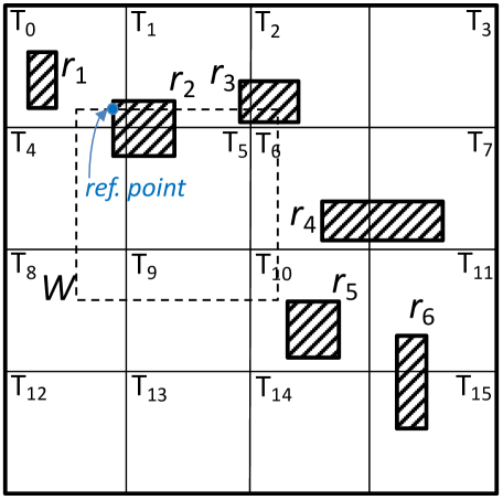
In this paper, we address an inherent problem that SOP indices have: potential duplicate query results. For example, consider the rectangular objects depicted in Figure 1, partitioned using a 4$\times$4 grid. Some objects are assigned to multiple tiles. Given a query range (e.g., $W$), a replicated object (e.g., $r_{2}$) may be identified as query result multiple times (e.g., at tiles $T_{0}$, $T_{1}$, $T_{4}$, and $T_{5}$). The classic, but slow, approach to eliminate duplicates is to hash the query results and identify duplicates at each bucket [17]. The state-of-the-art approach [18], used in most big spatial data management systems [6], computes, for each query result $r_{i}$ found in a partition $T$, a reference point of the intersection between $r_{i}$ and the query window $W$ (e.g., the upper-left corner in Figure 1). If the reference point is inside $T$, then $r_{i}$ is reported, otherwise it is ignored. Since the reference point can only be inside one partition, no duplicate results are reported. Although this method avoids hashing, we still have to bear the cost of finding duplicate results and computing the reference point for each of them.

tile primary partitioning secondary partitioning $T_{0}$ $\{r_{1},r_{2}\}$ $A=\{r_{1},r_{2}\}$ $T_{1}$ $\{r_{2},r_{3}\}$ $A=\{r_{3}\}$, $C=\{r_{2}\}$ $T_{2}$ $\{r_{3}\}$ $C=\{r_{3}\}$ $T_{4}$ $\{r_{2}\}$ $B=\{r_{2}\}$ $T_{5}$ $\{r_{2}\}$ $D=\{r_{2}\}$ $T_{6}$ $\{r_{4}\}$ $A=\{r_{4}\}$ $T_{7}$ $\{r_{4}\}$ $C=\{r_{4}\}$ $T_{10}$ $\{r_{5}\}$ $A=\{r_{5}\}$ $T_{11}$ $\{r_{6}\}$ $A=\{r_{6}\}$ $T_{15}$ $\{r_{6}\}$ $B=\{r_{6}\}$

Figure 1: Example of partitioning and object classes

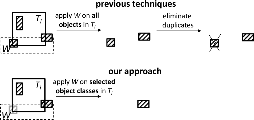
Contributions. In Section 3, we propose a secondary partitioning technique for SOP indices, which improves their performance significantly, by avoiding the generation and elimination of duplicate results. Our approach (i) is extremely easy to implement, (ii) it can be used by any SOP index, and (iii) it can be directly implemented in big spatial data management systems [6]. In a nutshell, we divide the objects which are assigned to each partition $T$ into four classes $A,B,C,D$. Objects in class $A$ begin inside $T$ in both dimensions, objects in class $B$ start inside $T$ in dimension $x$ only, objects in class $C$ start inside $T$ in dimension $y$ only, and objects in class $D$ start before $T$ in both dimensions. Figure 1 (column “secondary partitioning”) exemplifies how the objects are divided into classes. During query evaluation, for each partition $T$ which intersects the query range, we access only the object classes in $T$ that are guaranteed not to produce duplicate results. For example, in tile $T_{1}$ of Figure 1, we will not access class $C$, because query $W$ starts before $T_{1}$ in dimension $x$; i.e., any object in class $C$ of $T_{1}$ that intersects $W$ (like $r_{2}$) should also intersect $W$ in the previous tile $T_{0}$. In Section 4.1, we explain in detail how range queries are evaluated by our scheme and show how redundant computations and duplicate checks can be avoided overall. Figure 2 illustrates, for range queries, the difference between our approach and the de-duplication process followed by previous work [18, 17]; while all previous approaches evaluate queries on all objects of each partition and then eliminate possible duplicates, we process only a subset of objects in each partition that cannot be duplicates and we do not perform any de-duplication.

Figure 2: Comparing our approach to previous work

Besides duplicate avoidance, our technique can also facilitate reducing number of required comparisons per rectangle to at most one per dimension (Section 4.2). In Sec. 5, we turn our focus to spatial intersection joins. We first discuss join evaluation for two datasets that are primarily indexed by identical grids. To avoid duplicate results, we show that, for each tile, it suffices to evaluate 9 out of the 16 possible joins between the pairs of secondary partitions in the tile. We also show how to optimize the join phase of PBSM, by specialized plane-sweep routines for the different cases of joined sub-partitions (classes) and by avoidance of redundant comparisons. Finally, we investigate join evaluation when one or both joined inputs have already been indexed and how to process joins of datasets that have been partitioned using a different grid.

In Section 6, we evaluate our proposal experimentally using large publicly available real datasets and synthetic ones. Our experiments show that main-memory grids are superior to alternative SOP and DOP indices. More importantly, we show that when we replace the state-of-the-art duplicate elimination technique [18] by our secondary partitioning technique, the performance of grid-based indexing is improved by up to a few times.

This paper extends of our work in [19] to address spatial intersection joins. For the interest of space, some content from [19] is omitted from this version (storage decomposition optimization, handling of distance range queries, refinement step, batch query processing).

2 Related Work

2.1 Indexing Non-point Spatial Objects

Spatial queries are typically processed in two steps [1], following a filtering-and-refinement framework. During filtering, the query is applied on the MBRs, which approximate the objects. During refinement, the exact representations of the candidates are accessed and tested against the query predicate. Spatial indices are applied in the filtering step; hence, they manage MBRs instead of exact geometries.

Depending on the nature of the partitioning, spatial indices are classified into two classes [20]. Space-oriented partitioning (SOP) indices divide the space into disjoint partitions and were originally designed for point data. A grid [21], which divides the space into cells (partitions) using axis-parallel lines, is the simplest SOP index. Hierarchical indices in this category are the kd-tree [22] and the quad-tree [23],[24]. SOP can also be used for non-point objects; in this case, objects whose extent overlaps with multiple partitions are replicated (or clipped) in each of them [25].

Due to object replication, the same query results may be detected in multiple partitions intersecting the query and result deduplication should be applied [17]. Dittrich and Seeger [18] avoid duplicate results by computing a reference point of the intersection area between each result and the query range. If the reference point is inside the partition, then the result is reported, otherwise it is eliminated.

Indices based on data-oriented partitioning (DOP) allow the extents of the partitions to overlap and ensure that their contents are disjoint (i.e., each object is assigned to exactly one partition); hence, there is no need for result de-duplication. Variants of the R-tree [10] (e.g., the R*-tree [26]) are the most popular methods in this class. The R-tree is a disk-based, height-balanced tree, which generalizes the B⁺-tree in the multi-dimensional space and hierarchically groups object MBRs to blocks. The CR-tree [27] is an optimized R-tree for the memory hierarchy. BLOCK [20] is a main-memory DOP index, which uses a hierarchy of grids. R*-Grove [28] is a spatial partitioning, which builds on the split algorithm of R*-tree to define full blocks and balanced partitions for distributed big data.

Following a recent trend on relational data [29], learned indices for spatial data were proposed [30, 31, 32, 33, 34]. These indices are not directly comparable to our work, as they handle point data (with no obvious extension to non-point data) and their goal is to minimize the I/O cost.

2.2 Spatial Joins

A plane-sweep algorithm [35, 36] which computes rectangle intersections, is the most common approach for in-memory spatial joins. Brinkhoff et al. [37] present an forward sweep variant, which does not use any data structures. For datasets too large to fit in memory, data partitioning has been used in a divide-and-conquer fashion, such that inputs are split into smaller subsets which can be then joined fast in memory. A partition from input $R$ is then joined with a partition from $S$ only if their MBRs intersect. Partitioning-based approaches are divided in two categories. Single-assignment, multi-join (SAMJ) methods assign each object to exactly one partition, similar to DOP; then, a partition from one input may be joined with multiple partitions from the other. The R-tree Join algorithm [37] is a classic SAMJ approach, where both inputs are indexed by an R-tree.

On the other hand, multi-assignment, single-join (MASJ) methods, inspired by SOP, use identical and disjoint spatial partitions for both datasets. An object is assigned to every partition it spatially intersects and each partition from one input is joined with exactly one partition from the other. Partition-based Spatial Merge Join (PBSM) [38], the state-of-the-art MASJ method [39, 40], divides the space by a regular grid. For each spatial partition, PBSM accesses the objects from both inputs and performs the small join in memory (e.g., using plane-sweep). Duplicate join results are eliminated, using the reference point technique [18]). Other MASJ approaches include Spatial Hash Join [41] and Scalable Sweeping-Based Spatial Join [36].

In-memory methods also utilize partitioning to accelerate the join computation. TOUCH [42] first bulk-loads an R-tree for one of the inputs, using STR packing [43]. Then, all objects from the second input are assigned to buckets corresponding to the non-leaf nodes of the tree. Finally, each bucket is joined with the subtree rooted at the corresponding node, as in [44]. A comparison of spatial join algorithms for in-memory data [39] shows that PBSM and TOUCH perform best. Tauheed et al. [45] suggest an analytical model for configuring the grid of PBSM-like join processing.

2.3 Parallel and Distributed Data Management

With the advent of Hadoop, research on spatial data management has shifted to developing distributed systems for spatial data [46, 2, 3, 47, 4, 5]. Spatial data in Hadoop-GIS [2] are partitioned using a hierarchical grid, wherein high density tiles are split to smaller ones. The nodes of the cluster share a global tile index which can be used to find the HDFS files where the contents of the tiles are stored. Spatial queries are implemented as MapReduce workloads. SpatialHadoop [3], offers different options for partitioning (i.e., grid based, R-tree based, quad-tree based, etc.) The Master node holds a global spatial index for the MBRs of each of the HDFS file blocks. A local index is built at each physical partition and used by map tasks.

Spark-based implementations of spatial data management systems [47, 4, 5],[48] apply similar partitioning approaches. The main difference to Hadoop-based systems is that data, indices, and intermediate results are shared in the memories of all nodes in the cluster as RDDs. Unlike SpatialSpark [47], GeoSpark (now, Apache Sedona) [5] and Beast [48] which are built on top of Spark, Simba [4] has its own native query engine and query optimizer, but does not support non-point geometries. Pandey et al. [6] conduct a comparison between big spatial data analytics systems.

Distributed spatial data management systems focus on data partitioning and not on query evaluation at each partition. Emphasis is given on scaling out, rather than reducing the computational cost per node. On the other hand, we focus on in-memory spatial data management and scaling up, by reducing the computational cost of spatial query evaluation. Still, our ideas are readily applicable in share-nothing systems, where each spatial partition is independent and does not need input from others to produce results.

3 Two-layer Spatial Partitioning

In this section, we present our secondary partitioning approach for SOP spatial indices. Although our approach can be used in any SOP index, we will present it in the context of a regular grid, which divides the space into $N\times M$ disjoint spatial partitions, called tiles. An object $o$ is assigned to a tile $T$ iff $MBR(o)$ and $T$ intersect. For each tile $T$, we keep a list of (MBR, object-id) pairs that are assigned to $T$. The actual geometries of objects are stored separately and retrieved on-demand, based on their id’s. If the spatial distribution of objects is not uniform and there are many empty tiles, to save memory, we use a hash-table to access non-empty tiles based on their coordinates.

Secondary Partitioning. We propose that the (MBR, object-id) pairs at each tile are further divided into four classes $A$, $B$, $C$, and $D$ (which are physically stored separately in memory). Let $r.x=[r.x_{l},r.x_{u}]$ be the projection of MBR $r$ on the $x$ axis and $r.y=[r.y_{l},r.y_{u}]$ $r$’s $y$-projection. Now, consider an MBR $r$ which is assigned to tile $T$.

• $r$ belongs to class $A$, if for every dimension $d\in\{x,y\}$, the begin value $r.d_{l}$ of $r$ falls into projection $T.d$, i.e., if $T.d_{l}\leq r.d_{l}$.

• $r$ belongs to class $B$ if $r.x$ begins inside $T.x$ and $r.y$ begins before $T.y$, i.e., if $T.x_{l}\leq r.x_{u}$ and $T.y_{l}>r.y_{l}$.

• $r$ belongs to class $C$ if $r.x$ begins before $T.x$ and $r.y$ begins inside $T.y$, i.e., if $T.x_{l}>r.x_{l}$ and $T.y_{l}\leq r.y_{l}$.

• $r$ belongs to class $D$ if both its $x$- and $y$-projections begin before $T$, i.e., if $T.x_{l}>r.x_{l}$ and $T.y_{l}>r.y_{l}$.

Figure 3 illustrates examples of rectangles in a tile $T$ that belong to the four different classes. During data partitioning, when a rectangle $r$ is assigned to a tile $T$, we identify its class and place it to the corresponding division. Note that a rectangle can belong to class $A$ of just one tile, while it can belong to other classes (in other tiles) an arbitrary number of times. We denote the secondary partitions of tile $T$ which store the MBRs of classes $A$, $B$, $C$, and $D$, by $T^{A}$, $T^{B}$, $T^{C}$, and $T^{D}$, respectively. Table I summarizes the notation used frequently in the paper.

Figure 3: The four classes of rectangles assigned to a tile $T$.

TABLE I: Table of notations

Notation	Description
$W$	query window
$r.d=[r.d_{l},r.d_{u}]$	projection of rectangle $r$ at dimension $d\in\{x,y\}$
$T^{X}$	secondary partition of tile $T$ holding MBRs in class $X\in\{A,B,C,D\}$
$prev(T,d)$	previous tile to $T$ in dimension $d\in\{x,y\}$

4 Range Query Evaluation

In this section, we show how the secondary partitions at each tile $T$ can be used to avoid the generation and elimination of duplicate query results. We discuss the case of rectangular queries $W$ (window queries) and focus on the filtering step of the evaluation; details on non-rectangular queries and on the refinement step can be found in [19].

First, the tiles which intersect $W$ in a $N\times M$ regular grid can be found in $O(1)$ time, by algebraic operations. Specifically, assuming that tile $T_{i,j}$ is at the $i$-th row and at the $j$-th column of the grid, the tiles which intersect $W$ are all tiles $T_{i,j}$, for which $\lfloor W.x_{l}/N\rfloor\leq i\leq\lfloor W.x_{u}/N\rfloor$ and $\lfloor W.y_{l}/M\rfloor\leq j\leq\lfloor W.y_{u}/M\rfloor$. We now explain in detail, for each tile $T$ that intersects $W$, which classes of rectangles should be accessed and which computations are necessary for determining whether each rectangle $r$ intersects $W$.

4.1 Selecting relevant classes

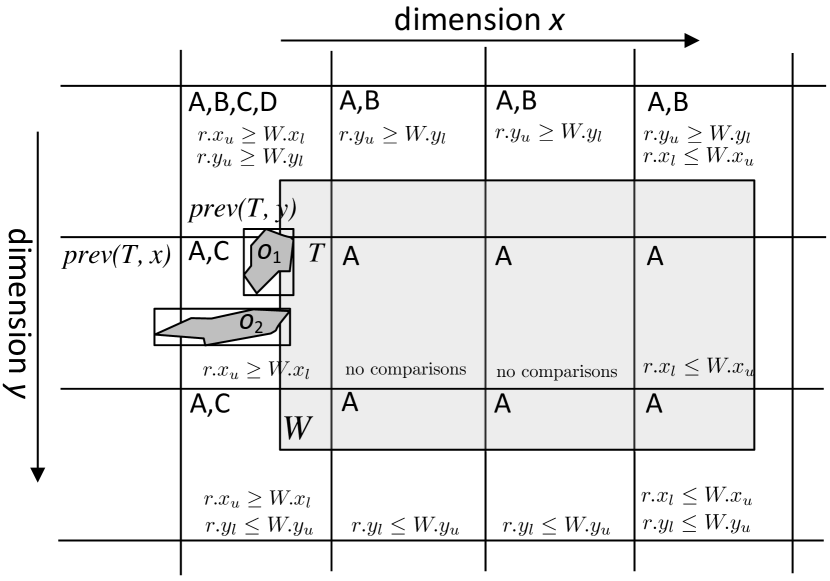
For a tile $T$, let $prev(T,d)$ denote the tile which is right before $T$ in dimension $d$ and has exactly the same projection as $T$ in the other dimension. For example, in Figure 4, $prev(T,x)$ (resp. $prev(T,y)$) is the tile right before $T$ in dimension $x$ (resp. $y$). Given a window query $W$, the following lemmas determine the classes of rectangles in $T$ which should be disregarded, because they can only produce duplicate results.

Lemma 1

If the query range $W$ intersects tile $T$ and $W$ starts before $T$ in dimension $x$, then secondary partitions $T^{C}$ and $T^{D}$ should be disregarded.

Proof. Consider a rectangle $r$ in class $C$ or class $D$ of tile $T$, i.e., $r\in T^{C}$ or $r\in T^{D}$. Rectangle $r$ should also be assigned to the previous tile $prev(T,x)$ to $T$ in dimension $x$, because it belongs to class $C$ or $D$ of $T$. If $r$ intersects $W$ in $T$, then $r$ should also intersect $W$ in $prev(T,x)$, because $W$ also starts before $T$ in dimension $x$. Hence, examining and reporting $r$ in tile $T$ would produce a duplicate, since the same result can also be identified in tile $prev(T,x)$. $\square$

Lemma 2

If $W$ intersects tile $T$ and $W$ starts before $T$ in dimension $y$, then secondary partitions $T^{B}$ and $T^{D}$ should be disregarded.

Lemma 2 can be proved by replacing $x$ by $y$ and $C$ by $B$ in the proof of Lemma 1. The two lemmas are combined to exclude all classes $B$, $C$, and $D$ if $W$ starts before $T$ in both dimensions. To illustrate the lemmas, consider tile $T$ in Figure 4. In addition, consider the MBRs of objects $o_{1}$ and $o_{2}$, which belong to secondary partitions $T^{B}$ and $T^{C}$, respectively. $MBR(o_{1})$ should be ignored when processing $T$ because it belongs to class $B$ and $W$ starts before $T$ in dimension $y$ (Lemma 2). Indeed, $MBR(o_{1})$ intersects $W$ also in tile $prev(T,y)$ which is right above $W$. On the other hand, $W$ does not start before $T$ in dimension $x$, i.e., Lemma 1 does not apply for tile $T$. This means that $MBR(o_{2})\in T^{C}$ will be found to intersect $W$. Figure 4 shows, in the top-left corner of each tile $T$ intersected by $W$, the object classes in $T$ that should be examined (the remaining classes can be disregarded). Observe that we have to consider all objects in just one tile (the one containing point $(W.x_{l},W.y_{l})$). For the majority of tiles, we only have to examine secondary partition $T^{A}$.

Figure 4: Examples of object classes and comparisons

4.2 Minimizing the number of comparisons

We now turn our attention to minimizing the number of comparisons needed for each secondary partition that has to be checked (i.e., those not eliminated by Lemmas 1 and 2). For a rectangle $r$ in a tile $T$ to intersect the query window $W$, $r.x$ should intersect $W.x$ and $r.y$ should intersect $W.y$. Hence, to test whether $x$ intersects $W$, we need at most four comparisons (i.e., $r$ and $W$ do not intersect, iff $r.x_{u}<W.x_{l}$ or $r.x_{l}>W.x_{u}$ or $r.y_{u}<W.y_{l}$ or $r.y_{l}>W.y_{u}$).

A direct observation that saves comparisons is that, if a tile $T$ is covered by the window $W$ in a dimension $d$, then we do not have to perform intersection tests in dimension $d$ for all rectangles in the relevant secondary partitions in $T$. In the example of Figure 4, we need to examine partitions $T^{A}$ and $T^{C}$ of tile $T$ (Lemma 2). For each rectangle $r$ in these partitions, we only have to verify if projections $r.x$ and $W.x$ intersect, because $r.y$ and $W.y$ definitely intersect (since $T.y$ is covered by $W.y$).

For the dimension(s) where $T$ is not covered by $W$, the following lemmas can be used to further reduce the necessary comparisons.

Lemma 3

If $W$ ends in tile $T$ and starts before $T$ in dimension $d$, then for a rectangle $r\in T$, $r$ intersects $W$ in dimension $d$ iff $r.d_{l}\leq W.d_{u}$.

Symmetrically, we can show:

Lemma 4

If $W$ starts in tile $T$ and ends after $T$ in dimension $d$, then for a rectangle $r\in T$, $r$ intersects $W$ in dimension $d$ iff $r.d_{u}\geq W.d_{l}$.

For example, in tile $T$ of Figure 4, we only have to test intersection in dimension $x$, as already explained. The intersection test can be reduced to a simple comparison, i.e., $r$ intersects $W$ iff $r.x_{u}\geq W.x_{l}$, due to Lemma 4. To demonstrate the impact of Lemmas 3 and 4, in each tile of the figure, we show the necessary comparisons. For the two tiles in the center, no comparisons are required because all MBRs (in class A) are guaranteed to intersect $W$. For the remaining two tiles, which intersect the border of $W$, we only have to perform at most one comparison per dimension, because $W$ either starts or ends at these tiles (and some of these tiles are totally covered by $W$ in one dimension). Contrast this to the four comparisons required in the general case for testing whether two rectangles (e.g., $r$ and $W$) intersect. Therefore, for range queries that cover multiple tiles, we have:

Corollary 1

For a window query $W$ that intersects more than one tile per dimension, at most two comparisons per rectangle in each relevant tile are required.

4.3 Overall approach

Algorithm 1 describes the steps of window query evaluation. Given a window $W$, we first identify the tiles $\mathcal{T}$ that intersect $W$ by simple algebraic operations, as discussed in the beginning of this section. Then, for each tile $T\in\mathcal{T}$, we identify the secondary partitions $\mathcal{P}_{T}$ that would not produce duplicates, using Lemmas 1 and 2. For each such secondary partition $T^{X}$, we find all rectangles that intersect $W$, by applying the techniques of Section 4.2 to reduce the necessary computations. Note that query evaluation at each tile $T$ (and each secondary partition) is totally independent from others and, hence, it is embarrassingly parallelizable.

1:grid $\mathcal{G}$, query window $W$

2:$\mathcal{T}$ = tiles in $\mathcal{G}$ that intersect $W$

3:for each tile $T\in\mathcal{T}$ do

4:    $\mathcal{P}_{T}$ = sub-partitions of $T$ relevant to $W$ $\triangleright$ Lemmas 1 & 2

5:    for each sub-partition $T^{X}\in\mathcal{P}_{T}$ do

6:         find all $r\in T^{X}$ that intersect $W$ $\triangleright$ Section 4.2

7:    end for

8:end for

Algorithm 1 Window query evaluation (filtering step)

Although we focus on indexing 2D MBRs in this paper, our secondary partitioning scheme can directly be used for minimum bounding boxes (MBBs) of arbitrary dimensionality $m$. In a nutshell, we need $2^{m}$ classes to re-partition an $m$-dimensional tile $T$, which indexes $m$-dimensional MBBs. For each tile $T$, if MBB $r$ intersects $T$, there are two cases for each dimension $d$: either $r$ begins inside $T$ ($r.d_{l}\geq T.d_{l}$) or before $T$ ($r.d_{l}<T.d_{l}$). Hence, there are $2^{m}$ cases (classes) in total. Lemmas 1 and 2 can be generalized to a lemma that prunes all classes corresponding to cases of MBBs that begin before $T$ in each dimension $d$, if $W$ begins before $T$ in that dimension. Lemmas 3 and 4 apply to any dimensionality.

5 Spatial Join Evaluation

We now turn our focus to the evaluation of spatial intersection joins. First, we discuss how our two-layer partitioning can be adopted to natively compute a spatial join, while avoiding the generation and elimination of duplicate results. Then, we elaborate on possible join strategies which use two-layer partitioning in different fashions. For illustration purposes, we discuss the above for regular grids; in Section 5.3, we consider other SOPs, e.g., the quad-tree.

5.1 Two-layer Partitioning Join

Assume that both inputs $R$, $S$ are indexed by our two-layer partitioning with identical grids. In the next subsection, we discuss the origins and details of such a setting, i.e., whether both or one of $R$, $S$ are (re)-indexed online. Under this setting, we can build upon the join phase of the PBSM algorithm [38] and apply a partition-to-partition join for each pair of partitions from $R$, $S$ from the same tile. Assuming that two partitions of size $n$, $m$ are joined, the join cost using plane-sweep is $O((n+m)\log(n+m))$, based on [37, 36].

5.1.1 The Mini-joins Breakdown

Given a tile $T$, let $R_{T}$ and $S_{T}$ be the partitions containing the object rectangles from datasets $R$ and $S$, respectively, that are assigned to $T$. $R_{T}$ is divided into rectangle classes $R^{A}_{T}$, $R^{B}_{T}$, $R^{C}_{T}$, and $R^{D}_{T}$, according to our two-layer partitioning scheme discussed in Section 3. Similarly, $S_{T}$ is divided into $S^{A}_{T}$, $S^{B}_{T}$, $S^{C}_{T}$, and $S^{D}_{T}$. Hence, the spatial join $R_{T}\bowtie S_{T}$ can now be decomposed into $4\cdot 4=16$ joins between classes of rectangles, i.e., $R^{A}_{T}\bowtie S^{A}_{T},R^{B}_{T}\bowtie S^{B}_{T},R^{B}_{T}\bowtie S^{C}_{T},\dots,R^{B}_{T}\bowtie S^{A}_{T},\dots$. We call these class-to-class joins, mini-joins. Figure 5 exemplifies the decomposition of the partition-to-partition join inside a tile $T$ into the 16 mini-joins.

Figure 5: Decomposition of tile $T$’s join into 16 mini-joins; $R$ rectangles filled in light gray color.

Looking deeper into these 16 cases, we can easily show that 7 out of these mini-joins (the shaded cases in the figure) produce only duplicate results, i.e., join results that will also be reported in another tile. For example, if two rectangles of class $B$ in tile $T$ intersect (i.e., the pair is contained in the result of $R^{B}_{T}\bowtie S^{B}_{T}$), then they will definitely intersect also in another tile above $T$. We can also show that the remaining 9 mini-joins produce only results that cannot be reported in any previous tile (in the $x$ or $y$ dimension or in both), but could be produced as duplicates in some of the 7 shaded joins in a tile after $T$ in one or both dimensions. Hence, we never evaluate the 7 shaded mini-joins and only evaluate the 9 remaining without the need of duplicate elimination.

5.1.2 Optimizations

Any spatial join algorithm can be utilized to evaluate the set of 9 mini-joins on each tile $T$; even a nested-loops approach. Following previous work on spatial joins [40, 38, 36], we adopt a plane-sweep join approach which is shown to perform significantly faster than nested-loops; specifically we adopt the plane-sweep algorithm in [37]. Algorithm 2 illustrates our plane-sweep mini-join. To apply the plane-sweep approach, the contents of each class are sorted on the sweeping dimension (Line 1). Without loss of generality, we consider $x$ as the sweeping dimension for the rest of this section, and so rectangles are sorted by $r.x_{l}$ and $s.x_{l}$. Sorting can take place also during the construction of the two-layer scheme, if an input dataset is partitioned online. For every pair $(r,s)$ determined by the sweeping process (i.e., rectangles whose projections on $x$ intersect), we test in Lines 6 and 14, if the rectangles also intersect in the second dimension $y$; i.e., if $r.y_{l}\leq s.y_{l}\leq r.y_{u}$ or $s.y_{l}\leq r.y_{l}\leq s.y_{u}$. To boost the computation of mini-joins, we next discuss how we can save on the comparisons performed for $(r,s)$ pairs, capitalizing on our second layer of partitioning.

1:classes of rectangles $R_{T}$ and $S_{T}$

2:sort $R_{T}$ and $S_{T}$ by $r.x_{l}$$\triangleright$ if not already sorted

3:while $R_{T}$ and $S_{T}$ not depleted do

4:    if $r.x_{l}<s.x_{l}$ then

5:         $s^{\prime}\leftarrow s$

6:         while $s^{\prime}\neq$ null and $r.x_{u}\geq s^{\prime}.x_{l}$ do

7:             if $r.y_{l}\!\leq\!s^{\prime}.y_{l}\!\leq\!r.y_{u}$ or $s^{\prime}.y_{l}\!\leq\!r.y_{l}\!\leq\!s^{\prime}.y_{u}$ then

8:                 output $(r,s^{\prime})$$\triangleright$ update result

9:             end if

10:             $s^{\prime}\leftarrow$ next rectangle in $S_{T}$$\triangleright$ scan forward

11:         end while

12:    else

13:         $r^{\prime}\leftarrow r$

14:         while $r^{\prime}\neq$ null and $s.x_{u}\geq r^{\prime}.x_{l}$ do

15:             if $r^{\prime}.y_{l}\!\leq\!s.y_{l}\!\leq\!r^{\prime}.y_{u}$ ​or​ $s.y_{l}\!\leq\!r^{\prime}.y_{l}\!\leq\!s.y_{u}$ then

16:                 output $(r^{\prime},s)$$\triangleright$ update result

17:             end if

18:             $r^{\prime}\leftarrow$ next rectangle in $R_{T}$$\triangleright$ scan forward

19:         end while

20:    end if

21:end while

Algorithm 2 Plane-sweep mini-join

Avoid unnecessary comparisons. There exist two ways to utilize the $A$, $B$, $C$, $D$ classes in each tile $T$ for avoiding unnecessary rectangle comparisons. To understand the first, consider the $R_{T}^{A}\bowtie S_{T}^{C}$ mini-join. By definition, all objects rectangles in $S_{T}^{C}$ precede the rectangles in $R_{T}^{A}$. In practice, this means that we can apply a simplified version of plane-sweep for $R_{T}^{A}\bowtie S_{T}^{C}$ which performs forward scans on $R_{T}^{A}$ for each rectangle in $S_{T}^{C}$, as the $r.x_{l}>s.x_{l}$ holds by definition. This modification will save on unnecessary comparisons between $r\in R_{T}^{A}$ and $s\in S_{T}^{C}$ objects and further will allow us to avoid sorting the $S_{T}^{C}$ class. Algorithm 3 presents this reduced version of the plane-sweep mini-join. We can apply the same principle also for $R_{T}^{A}\bowtie S_{T}^{C}$, $R_{T}^{C}\bowtie S_{T}^{A}$, $R_{T}^{A}\bowtie S_{T}^{D}$, $R_{T}^{D}\bowtie S_{T}^{A}$, $R_{T}^{B}\bowtie S_{T}^{C}$ and $R_{T}^{C}\bowtie S_{T}^{B}$. Overall, we do not need to sort the $R_{T}^{C}$, $R_{T}^{D}$, $S_{T}^{C}$, $S_{T}^{D}$ classes.

1:classes of rectangles $R_{T}$ and $S_{T}$

2:sort $R_{T}$ by $r.x_{l}$$\triangleright$ if not already sorted

3:while $S_{T}$ not depleted do

4:    $r^{\prime}\leftarrow r$

5:    while $r^{\prime}\neq$ null and $s.x_{u}\geq r^{\prime}.x_{l}$ do

6:         if $r^{\prime}.y_{l}\!\leq\!s.y_{l}\!\leq\!r^{\prime}.y_{u}$ or $s.y_{l}\!\leq\!r^{\prime}.y_{l}\!\leq\!s.y_{u}$ then

7:             output $(r^{\prime},s)$$\triangleright$ update result

8:         end if

9:         $r^{\prime}\leftarrow$ next rectangle in $R_{T}$$\triangleright$ scan forward

10:    end while

11:end while

Algorithm 3 Reduced plane-sweep mini-join

Besides the plane-sweep process, we can also avoid unnecessary comparisons when considering the second dimension (i.e., $y$). The idea is similar to Lemmas 3 and 4. Take as example, the $R_{T}^{A}\bowtie S_{T}^{B}$ mini-join. For every pair $(r,s)$ of intersecting object rectangles in $x$, determined by plane-sweep, the $s.y_{l}<r.y_{l}$ condition holds by definition. Hence, to determine whether $r$, $s$ intersect also in dimension $y$ we only need to check the $r.y_{l}<s.y_{u}$ condition. The same principle can be used for the $R_{T}^{A}\bowtie S_{T}^{D}$, $R_{T}^{B}\bowtie S_{T}^{A}$, $R_{T}^{D}\bowtie S_{T}^{A}$, $R_{T}^{B}\bowtie S_{T}^{C}$ and $R_{T}^{C}\bowtie S_{T}^{B}$ mini-joins. The following lemma summarizes this optimization for every object rectangle $r$ in classes $R_{T}^{B}$, $R_{T}^{D}$ with $s$ in classes $S_{T}^{A}$ and $S_{T}^{C}$; the other case is symmetric.

Lemma 5

If an object rectangle $r$ in tile $T$ starts before the tile in the $y$ dimension, i.e., $T.y_{l}>r.y_{l}$, then $r$ intersects all $s$ rectangles in $T$ that start after $T.y_{l}$ with $r.y_{u}>s.y_{l}$.

Avoid redundant comparisons.

(a) $S_{T}^{C}$ unsorted	(b) $S_{T}^{C}$ sorted

Figure 6: Avoiding redundant comparisons on $R^{A}_{T}\bowtie S^{C}_{T}$; $R$ rectangle filled in light gray color.

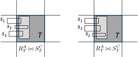
To illustrate this optimization, consider the $R^{A}_{T}\bowtie S^{C}_{T}$ mini-join and the rectangles in Figure 6(a). As already discussed, the reduced plane-sweep approach (Algorithm 3) does not sort the $S^{C}_{T}$ class, to evaluate this mini-join; by definition, the start $s.{x_{l}}$ for their contents precede the $r.x_{l}$ start of all rectangles in $R^{A}_{T}$. Hence, assume that the $S^{C}_{T}$ rectangles are examined in the $s_{1}$, $s_{2}$, $s_{3}$ order. Rectangles $s_{1}$ and $r$ intersect in the $x$ dimension as $s_{1}.x_{u}>r.x_{l}$ holds and so, they are next compared in the $y$ dimension. Algorithm 3 will similarly determine that both $s_{2}$ and $s_{3}$ also intersect $r$ in $x$ by checking $s_{2}.x_{u}>r.x_{l}$ and $s_{3}.x_{u}>r.x_{l}$, respectively. However, since $s_{2}.x_{u}>s_{1}.x_{u}$ and $s_{3}.x_{u}>s_{1}.x_{u}$ hold, the $s_{1}.x_{u}>r.x_{l}$ check for $s_{1}$ automatically implies that $s_{2}.x_{u}>r.x_{l}$ and $s_{3}.x_{u}>r.x_{l}$ also hold. In other words, we conducted two extra comparisons to determine the intersecting $(r,s_{2})$ and $(r,s_{3})$ pairs. To avoid such redundant comparisons, we can sort $S^{C}_{T}$ by $s.x_{u}$ which will essentially allow us to determine intersecting rectangles in batches. Figure 6(b) illustrates this idea; all three intersecting pairs can be determined after checking only $s_{1}$ against $r$. Algorithm 4 modifies Algorithm 3 accordingly. After identifying the first rectangle $s$ that intersects current $r^{\prime}$ in the $x$ dimension (Line 5), the algorithm pairs $r^{\prime}$ with every rectangle $s^{\prime}$ that follows $s$ in $S_{T}$ (Line 6).

1:classes of rectangles $R_{T}$ and $S_{T}$

2:sort $R_{T}$ by $r.x_{l}$$\triangleright$ if not already sorted

3:sort $S_{T}$ by $r.x_{u}$$\triangleright$ if not already sorted

4:while $S_{T}$ not depleted do

5:    $r^{\prime}\leftarrow r$

6:    while $r^{\prime}\neq$ null and $s.x_{u}\geq r^{\prime}.x_{l}$ do

7:         for each rectangle $s^{\prime}$ after $s$ in $S_{T}$ do$\triangleright$ batch

8:             if $r^{\prime}.y_{l}\!\leq\!s^{\prime}.y_{l}\!\leq\!\!r^{\prime}.y_{u}$ ​or​ $s^{\prime}.y_{l}\!\leq\!r^{\prime}.y_{l}\!\leq\!s^{\prime}.y_{u}$ then

9:                 output $(r^{\prime},s^{\prime})$$\triangleright$ update result

10:             end if

11:             $r^{\prime}\leftarrow$ next rectangle in $R_{T}$$\triangleright$ scan forward

12:         end for

13:    end while

14:end while

Algorithm 4 Reduced plane-sweep mini-join with batch outputting

5.2 Join Strategies

We last discuss different join strategies depending on the (pre)-existence of two-layer partitioning in the input. Following the classification in [1], we consider three settings.

5.2.1 Both Inputs Indexed

Under this setting, a two-layer partitioning already exists on each input dataset $R$, $S$ to answer other types of spatial queries, e.g., range queries. We distinguish between two cases with respect to the granularity of the pre-existing grids. If the two grids are identical, we can directly apply the mini-joins approach and its optimizations in Section 5.1.

If the pre-existing grids have different granularities, then the mini-joins approach is not directly applicable. A straightforward solution is to re-index one of the input datasets, e.g. $R$, by creating a temporary two-layer partitioning with a grid granularity that matches the grid on $S$, similar to [49]. In this context, a key question that naturally arises is which input we should re-index. Typically, we could select the dataset with either the smallest cardinality or the smallest average object extent, because such a decision is expected to incur the lowest online indexing cost. We elaborate on this decision in our experimental analysis.

Figure 7: Online grid transformation; $R$ partitioned by a $2\times 2$ grid, highlighted in blue, $S$ partitioned a $8\times 8$ grid, in black.

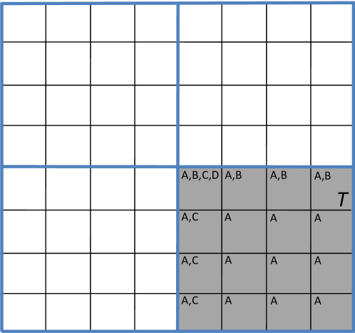
As an alternative, we also devise a new solution which completely eliminates the need to decide which input should be re-indexed and also significantly reduces the online indexing costs. For this purpose, the granularity of the pre-existing grids must be in a power of 2. If so, we can always define an online transformation of the finer grid to the coarser, by means of standard window range queries. Figure 7 exemplifies this transformation when $R$ is partitioned by a $2\times 2$ grid (colored in blue), and $S$ by a $8\times 8$ grid (in black). After overlaying the two grids, we observe that every tile $T$ in the $R$ grid overlaps a collection of exactly 16 adjacent tiles from the $S$ grid. Therefore, to re-partition $S$ to the $2\times 2$ grid of $R$, it suffices to compute the window queries defined by all tiles in the $R$ grid; the key idea is to determine the contents of the new $S^{A}_{T}$, $S^{B}_{T}$, $S^{C}_{T}$ and $S^{D}_{T}$ classes based on the results of every $T$ window query. For this purpose, we can utilize the original two-layer partitioning on $S$. Specifically, consider the shaded tile $T$ from the $R$ grid in Figure 7. Similar to Figure 4, we mark the relevant classes for each tile from the original $S$ grid that overlaps with the window query based on $T$, as discussed in Section 4. We can now construct $S^{A}_{T}$ by unifying the objects contained in the $A$ class of all overlapping tiles. For $S^{B}_{T}$, we consider only the contents of the $B$ class inside the top border overlapping tiles, while for $S^{C}_{T}$, the left border overlapping ones. Finally, $S^{D}_{T}$ is identical to the $D$ class inside the top left corner overlapping tile. The above process can be generalized for any two pre-existing grids of granularity $n\times n$ and $m\times m$, where $n>m$ and $n$, $m$ are powers of 2. Every tile in the second, coarser grid defines a window query that overlaps with exactly $(n/m)^{2}$ tiles from the first, finer one.

We developed two variants for the above transformation. The first constructs a temporary two-layer partitioning on input $S$ by matelializing the contents of each new $S^{A}_{T}$, $S^{B}_{T}$, $S^{C}_{T}$ and $S^{D}_{T}$ classes. After this, we can directly utilize the mini-joins approach in Section 5.1 to compute the $R\bowtie S$ spatial join. In contrast, the second variant never actually constructs this new two-layer scheme on input $S$. Instead, we adjust the joining process in Section 5.1 to determine on-the-fly which tiles from the original grid on $S$ should be used in the mini-joins. Specifically, the $R^{A}_{T}\bowtie S^{A}_{T}$ is further decomposed to $(n/m)^{2}$ mini-joins, i.e., $R^{A}_{T}\bowtie S^{A}_{T}=\bigcup_{i}R^{A}_{T}\bowtie S^{A}_{T_{i}}$, where $T_{i}$ denotes one of the $(n/m)^{2}$ tiles from the original $S$ grid overlapping with tile $T$ from the $R$ grid. In the same spirit, $R^{A}_{T}\bowtie S^{B}_{T}$, $R^{A}_{T}\bowtie S^{B}_{T}$, $R^{B}_{T}\bowtie S^{C}_{T}$ and $R^{C}_{T}\bowtie S^{B}_{T}$ are decomposed into $(n/m)$ mini-joins, while $R^{B}_{T}\bowtie S^{A}_{T}$, $R^{C}_{T}\bowtie S^{A}_{T}$ and $R^{D}_{T}\bowtie S^{A}_{T}$ into $(n/m)^{2}$. In Section 6, we compare the two variants and break down their total execution time.

5.2.2 One Input Indexed

Under this setting, a two-layer partitioning already exists only for one of the input datasets; without loss of generality, assume for $S$. In this case, there exist two alternative approaches for computing the $R\bowtie S$ spatial join. The first is to construct a temporary two-layer partitioning on $R$ with a grid of identical granularity to the grid on $S$, such that we can directly apply the joining process in Section 5.1. Despite its simplicity, this approach may exhibit high total execution times because of the online indexing cost.

Alternatively, we can adopt an index-based join approach. According to this, we scan the contents of the $R$ input and probe the index on $S$. Specifically, we issue a window range query for each object rectangle $r$ in $R$ which is evaluated using the two-layer partitioning on $S$. To further enhance the performance of this approach, we can examine the objects in $R$ according to their position in space, instead in a random order, e.g., by first partitioning them online with a grid or using a space filling curve. This way, window queries for objects in $R$ that overlap neighboring parts of the $S$ grid are evaluated in nearby timestamps, improving the cache locality.

5.2.3 No Input Indexed

Under this setting, none of the input datasets $R$, $S$ is indexed. In this case, we can partition both inputs under identical grids to construct two temporary two-layer partitioning schemes and then directly apply the mini-joins approach from Section 5.1.

Since both inputs are indexed online, we can further enhance the join process by adopting a specialized storage optimization. Note that such an optimization cannot be utilized for the settings discussed in the previous sections, as at least one of the two-layer schemes used for the join, pre-exists in order to evaluate other types of queries. Essentially, if we enforce this optimization, the resulting two-layer partitioning will no longer be able to fulfil its original purpose.

Conventionally, each rectangle $r$ is stored as a quintuple $\langle id,r.x_{l},r.x_{u},r.y_{l},r.y_{u}\rangle$. Assuming $x$ as the sweeping dimension (the other case is symmetric), $r.y_{l}$ is never needed for classes $B$ and $D$ when we check whether two rectangles intersect also in the $y$ dimension, i.e., in Lines 6 and 14 of Algorithm 2, Line 5 of Algorithm 3 and in Line 7 of Algorithm 4. This is because all contained rectangles start before the start of the tile in $y$. In fact, for class $D$, we do not need $r.x_{l}$ either, since $D$ is only joined to an $A$ class from the other input $S$ and its contents always precede those $S$ rectangles in both dimensions. Hence, a temporary two-layer partitioning stores all information for rectangles in classes $A$, $C$ but $\langle id,r.x_{l},r.x_{u},r.y_{u}\rangle$ for $B$ and $\langle id,r.x_{u},r.y_{u}\rangle$ for $C$, which reduces the online partitioning costs.

5.3 Extension to other SOPs

The two-layer partitioning join in Section 5.1 is directly applicable to any SOP, provided that identical partitions of the space (defined either offline or online) are considered for both inputs. Similarly, the index-based join approach can be applied when one of the inputs is indexed any SOP, enhanced with our two-layer partitioning. Lastly, when both inputs are indexed by the same SOP but under a different set of partitions, the re-partitioning approach in Section 5.2.1 can be applied when there exists an alignment among the partitions; e.g., in quad-trees, for each a quadrant (of a coarse granularity) in one input that entirely covers a set of finer quadrants from the other.

6 Experimental Evaluation

Our analysis was conducted on a machine with 384 GBs of RAM and a dual Intel(R) Xeon(R) CPU E5-2630 v4 clocked at 2.20GHz running CentOS Linux 7.6.1810. All methods were implemented in C++, compiled using gcc (v4.8.5) with flags -O3, -mavx and -march=native.

TABLE II: Real-world datasets used in the experiments

dataset	type	cardinality	avg. relative [%]
			$x$-extent	$y$-extent
ROADS	linestrings	$19$M	$0.007$	$0.013$
EDGES	polygons	$69$M	$0.003$	$0.005$
ZCTA5	polygons	$33$K	$1.7$	$2.052$
TIGER	mixed	$97$M	$0.004$	$0.008$

Datasets. We experimented with publicly available Tiger 2015 datasets [3], downloaded from http://spatialhadoop.cs.umn.edu/datasets.html. Their statistics are summarized in Table II. The fourth dataset resulted by merging all polygon and linestring Tiger 2015 objects. The objects in each dataset were normalized so that the coordinates in each dimension take values inside $[0,1]$. The last two columns of the table are the relative (over the entire space) average length for every object’s MBR at each axis. To test the robustness of our index, we also experimented with synthetically generated datasets with rectangles of uniform and zipfian spatial distribution. Table III shows the parameters used in data generation. The coordinates in each dimension take values in $[0,1]$ and all generated rectangles in a dataset have the same area. The width to height ratio of each rectangle was generated randomly in the range $[0.25,4]$ to avoid unnaturally narrow rectangles.

TABLE III: Synthetic datasets (MBRs) used in the experiments

parameter	values	default
cardinality	1M, 5M, 10M, 50M, 100M	10M
area	$10^{-\infty}$, $10^{-14}$, $10^{-12}$, $10^{-10}$, $10^{-8}$, $10^{-6}$	$10^{-10}$
distribution	Uniform or Zipfian ($a=1$)	—

Methods. We implemented our secondary partitioning approach denoted by $\mathsf{2\mbox{-}layer}$ as part of a main-memory regular grid spatial index. For each tile $T$ of the grid, $\mathsf{2\mbox{-}layer}$ divides the (MBR, id) pairs assigned to $T$ into four secondary partitions ($T^{A}$, $T^{B}$, $T^{C}$, $T^{D}$), as discussed in Section 3.

TABLE IV: Test methods and their throughput (range queries)

type	index	details	throughput [queries/sec]
			ROADS	EDGES
SOP	$\mathsf{2\mbox{-}layer}$	Section 3	30981	9406
	$\mathsf{1\mbox{-}layer}$	grid with [18]	12597	4403
	$\mathsf{quad\mbox{-}tree}$	[23] using [18]	10949	3640
	$\mathsf{quad\mbox{-}tree}$, $\mathsf{2\mbox{-}layer}$	[23] + Section 3	16883	5831
DOP	$\mathsf{R\mbox{-}tree}$	[43] (boost.org)	7888	2011
	$\mathsf{R\mbox{*-}tree}$	[26] (boost.org)	6415	1610
	$\mathsf{BLOCK}$	[20]	$<1$	$<1$
	$\mathsf{MXCIF\mbox{ }\mathsf{quad\mbox{-}tree}}$	[50]	8	2

We considered both SOP and DOP competitors to our $\mathsf{2\mbox{-}layer}$ , summarized in Table IV. First regarding SOPs, the $\mathsf{1\mbox{-}layer}$ index is an in-memory grid with identical primary partitioning as our $\mathsf{2\mbox{-}layer}$, but uses the reference point approach [18] to perform duplicate elimination. Comparing $\mathsf{1\mbox{-}layer}$ to $\mathsf{2\mbox{-}layer}$ shows the benefit of our secondary partitioning scheme and the techniques we propose in Section 4 for duplicate avoidance and minimization of comparisons. The second SOP competitor is a $\mathsf{quad\mbox{-}tree}$ implementation, which assigns each object MBR to all quadrants it intersects. As soon as the contents of a quadrant exceed a predefined maximum capacity (set to 1000, after tuning), the quadrant is split to four; the rectangles are then re-distributed in the four generated children and replicated if they span the division borders. To avoid extensive splitting of $\mathsf{quad\mbox{-}tree}$ nodes in the case of extremely skewed data, a maximum tree depth (=12) is set. The reference point approach [18] is also used for duplicate elimination. We also implemented a version of $\mathsf{quad\mbox{-}tree}$ that uses our approach instead of [18]. Regarding DOPs, we used two implementations of in-memory R-trees from the highly optimized Boost. Geometry library (boost.org); an STR-bulkloaded [43] (denoted for simplicity as $\mathsf{R\mbox{-}tree}$) and an $\mathsf{R\mbox{*-}tree}$ [26]. Both trees have a fanout of 16 for inner and leaf nodes; this configuration is reported to perform the best (we also confirmed this by testing). The next DOP competitor is $\mathsf{BLOCK}$; the implementation was kindly provided by the authors of [20]. Finally, we also implemented and tested the $\mathsf{MXCIF\mbox{ }\mathsf{quad\mbox{-}tree}}$ for non-point data [50], which stores each object at the lowest-level quadrant which covers the object. All compared methods are listed in Table IV.

Queries. To study the evaluation of range queries, we experimented with window queries which apply on non-empty areas of the map (i.e., they always return results). We vary their relative area as a percentage of the entire data space, inside the $\{0.01,0.05,0.1,0.5,1\}$ value range (default value $0.1$% of the area of the map). Queries on synthetic data follow the same spatial distribution as the data.

6.1 Indexing and Tuning

We first investigate the index building cost and tuning. The first two plots of Figure 8 compare the indexing times of $\mathsf{1\mbox{-}layer}$ and $\mathsf{2\mbox{-}layer}$ on ROADS and EDGES, while varying the granularity of the grid partitioning. Indexing sizes are omitted due to lack of space. Both indices occupy the same space, regardless of employing the secondary partitioning or not, as exactly the same number of object MBRs (originals and replicas) are stored. Note that the index sizes do not grow too much with the grid granularity, from 0.8 to 1.2GBs for ROADS, from 2.5 to 3GBs for EDGES, which means that MBR replication is not excessive. Naturally, the indexing cost for both indices rises as we increase the granularity of the grid. In terms of indexing time, $\mathsf{2\mbox{-}layer}$ is only slightly more expensive than $\mathsf{1\mbox{-}layer}$. The construction costs for the two quadtrees (not shown) are 7s and 28.2s, respectively, and their sizes are similar to those of the corresponding $\mathsf{1\mbox{-}layer}$ indices. The sizes of the packed R-trees (not shown) are about the same as the sizes of the corresponding $\mathsf{1\mbox{-}layer}$, $\mathsf{2\mbox{-}layer}$ indices, indicating that the replication ratio of our index is low. In addition, the bulk loading costs of the R-trees are 5.2s and 19.5s for the two datasets, respectively, both higher than the construction cost of $\mathsf{2\mbox{-}layer}$.

ROADS	EDGES
partitions per dimension [$\times$1000]	partitions per dimension [$\times$1000]
partitions per dimension [$\times$1000]	partitions per dimension [$\times$1000]

Figure 8: Building & tuning grid-based indices (range queries)

The last two plots of Figure 8 compare the window query throughputs of $\mathsf{1\mbox{-}layer}$ and $\mathsf{2\mbox{-}layer}$ for different grid granularities. The two methods achieve their best throughputs when several thousands of partitions per dimension are used. Observe that employing our secondary partitioning significantly enhances query processing; $\mathsf{2\mbox{-}layer}$ always outperforms $\mathsf{1\mbox{-}layer}$ by a wide margin (2x–3x). It is worth noting that $\mathsf{1\mbox{-}layer}$ uses the comparisons reduction optimization described in Section 4.2, meaning that the performance gap is due to our secondary partitioning. Specifically, our approach outperforms the state-of-the-art reference point method for result deduplication [18] used in $\mathsf{1\mbox{-}layer}$ by a factor of at least 2. For a wide range of granularities (i.e., 2000 to 5000 partitions per dimension), the throughput of both methods does not change significantly meaning that finding the best granularity is not crucial to query performance. We observed similar trends on the TIGER and on the synthetic datasets (not shown due to lack of space). As a rule of the thumb, we can set the extent of a grid cell in each dimension, 10 times larger than the average extent of the objects in that dimension. For the rest of our analysis, we used the best granularity for $\mathsf{1\mbox{-}layer}$ and $\mathsf{2\mbox{-}layer}$, see Table V.

TABLE V: Best granularities (partitions per dimension); in parenthesis, the power of 2 used for the transformation-based methods in Figure 12.

index	ROADS	EDGES	ZTCA5	TIGER	Uniform	Zipfian
$\mathsf{1\mbox{-}layer}$	1000	3000	not used	1000	500	3000
$\mathsf{2\mbox{-}layer}$	3000 ($2^{11}$)	5000 ($2^{12}$)	400 ($2^{8}$)	5300	450	3000

$\mathsf{R\mbox{-}tree}$   $\mathsf{quad\mbox{-}tree}$   $\mathsf{1\mbox{-}layer}$   $\mathsf{2\mbox{-}layer}$  

ROADS
query relative area [%]	query selectivity [%]
EDGES
query relative area [%]	query selectivity [%]
TIGER
query relative area [%]	query selectivity [%]

Figure 9: Range queries: real datasets

6.2 Range Query Performance

We next compare our two-layer partitioning against competition on query throughput. Table IV reports the throughput (queries/sec) achieved by each index for 10K window queries (of average relative area 0.1% of the map) on ROADS and EDGES. $\mathsf{2\mbox{-}layer}$ outperforms the competition by a wide margin. Note that the performance of $\mathsf{quad\mbox{-}tree}$ is greatly improved by our secondary partitioning, which confirms that other SOPs besides grids can benefit from our approach. However, as $\mathsf{2\mbox{-}layer}$ is consistently more efficient than the $\mathsf{quad\mbox{-}tree}$ using our approach, we do not consider the latter in the rest of the experiments. $\mathsf{R\mbox{-}tree}$ is the most efficient DOP competitor, outperforming $\mathsf{R\mbox{*-}tree}$ (from the same library). $\mathsf{BLOCK}$ takes seconds to evaluate range queries on our datasets, which can be attributed to the fact that it is implemented for 3D objects. Similar, $\mathsf{MXCIF\mbox{ }\mathsf{quad\mbox{-}tree}}$ is orders of magnitude slower than the $\mathsf{R\mbox{-}tree}$. Under these, in the rest of the tests we only include $\mathsf{1\mbox{-}layer}$, $\mathsf{R\mbox{-}tree}$ and $\mathsf{quad\mbox{-}tree}$ indices as the key competitors to our $\mathsf{2\mbox{-}layer}$.

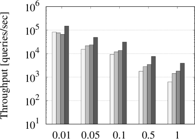
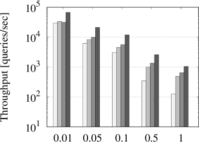
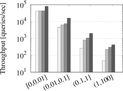
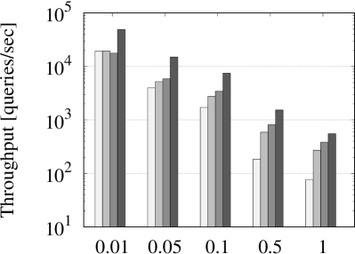
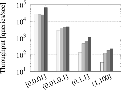
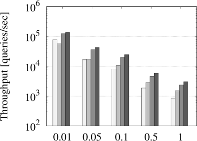
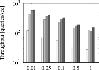
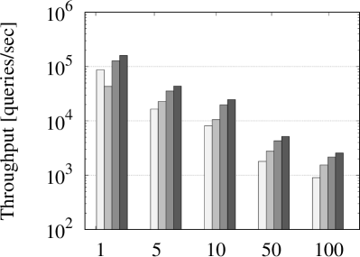
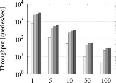
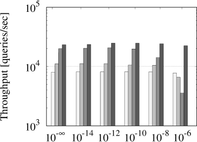
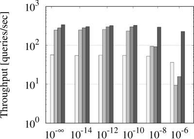
The first two columns of Figure 9 show the throughput of the four competitors for window queries of varying relative area and selectivity on the three real datasets. For the experiments of the second column, we collected the runtimes of all queries (regardless of their areas) and averaged them after grouping them by selectivity. Naturally, query processing is negatively affected by both factors. We also observe that $\mathsf{2\mbox{-}layer}$ is consistently much faster than the competition on all datasets and query areas. For each query, $\mathsf{2\mbox{-}layer}$ accesses the relevant partitions very fast (without the need of traversing a hierarchical index) and manage to drastically reduce the required number of computations. Figure 10 compares all methods for window queries on the synthetic datasets (for grid granularities, see Table V). In these experiments, we additionally vary the database size and the areas of the data objects. In terms of query throughput w.r.t. query area and selectivity, the trends are similar as those for the real data. In addition, the data cardinality does not affect the relative performance of the methods. Finally, we observe that $\mathsf{2\mbox{-}layer}$ is more robust to the area of the data objects compared to the competition. As the area grows, the replication to tiles increases, and so $\mathsf{1\mbox{-}layer}$ and $\mathsf{quad\mbox{-}tree}$ have to compute and eliminate more duplicate results. In contrast, $\mathsf{2\mbox{-}layer}$, with the help of our secondary partitioning, completely avoids the generation and elimination of duplicate results. On the other hand when the data area shrinks ($10^{-\infty}$ represents the case of extremely small rectangles that resemble points), the replication to tiles decreases. $\mathsf{1\mbox{-}layer}$ and the $\mathsf{quad\mbox{-}tree}$ still need to perform the extra comparison of the de-duplication reference test, which explains the stable advantage of $\mathsf{2\mbox{-}layer}$ .

$\mathsf{R\mbox{-}tree}$   $\mathsf{quad\mbox{-}tree}$   $\mathsf{1\mbox{-}layer}$   $\mathsf{2\mbox{-}layer}$

Uniform (default)	Zipfian (default)
query relative extent [%]	query relative extent [%]
data cardinality [$\times 10^{6}$]	data cardinality [$\times 10^{6}$]
data rectangle area	data rectangle area

Figure 10: Range queries: synthetic datasets

6.3 Updates Performance

We also demonstrate the superiority of our two-layer partitioning in updates. For this purpose, we conducted an experiment using the real datasets, where we first constructed the index by loading 90% of the data in batch and then measuring the cost of incrementally inserting the last 10% of the data. Table VI compares the total update costs of the competitor indices. $\mathsf{R\mbox{-}tree}$ is two orders of magnitude slower than the baseline $\mathsf{1\mbox{-}layer}$ index and the cost of updates on $\mathsf{2\mbox{-}layer}$ is only a bit higher compared to the update cost on $\mathsf{1\mbox{-}layer}$. Updates on $\mathsf{quad\mbox{-}tree}$ are also slower compared to $\mathsf{1\mbox{-}layer}$ and $\mathsf{2\mbox{-}layer}$, due to the tree traversal.

TABLE VI: Total update cost (sec)

dataset	$\mathsf{R\mbox{-}tree}$	$\mathsf{quad\mbox{-}tree}$	$\mathsf{1\mbox{-}layer}$	$\mathsf{2\mbox{-}layer}$
ROADS	5.34	0.76	0.059	0.068
EDGES	19.8	2.89	0.267	0.382
TIGER	33.91	4.63	0.459	0.634

6.4 Spatial Join Performance

6.4.1 Two-layer Partitioning Join

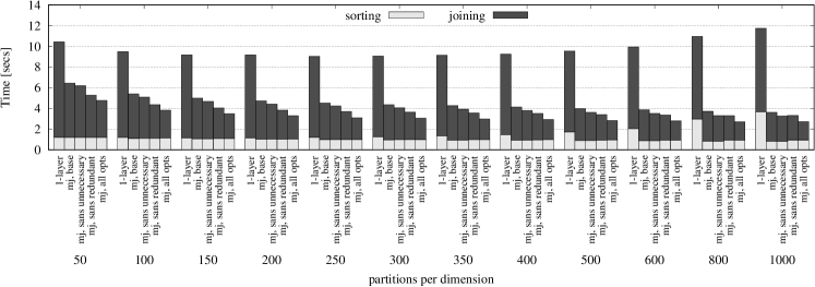
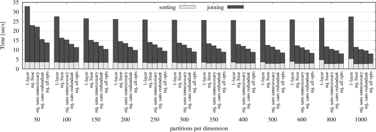
We first study the impact of our second layer of partitioning to the join computation. As discussed in Section 5.1, we assume that both input datasets are already indexed and that identical grids exist as the first layer of partitioning. We implemented the mj, base method on top of our $\mathsf{2\mbox{-}layer}$ scheme, as our basic mini-joins solution which adopts the mini-joins breakdown from Section 5.1.1 and the plane-sweep join approach from Section 5.1.2. To demonstrate the effect of the comparison-saving optimizations from Section 5.1.2, we also developed the mj, sans unecessary and mj, sans redundant variants, which extend mj, base. Last, we implemented a mini-joins solution with all optimizations activated, denoted by mj, all opts and $\mathsf{1\mbox{-}layer}$, a PBSM baseline solution that solely employs the first layer of partitioning.

Figure 11 reports the breakdown of the total execution time while varying the number of partitions per dimension for the ROADS $\bowtie$ ZCTA5 and EDGES $\bowtie$ ZCTA5 queries. Note that we excluded the offline partitioning time but included the sorting time needed for adopting plane-sweep and saving on redundant comparisons. The results clearly show the benefit of employing our second layer of partitioning and the mini-joins breakdown compared to $\mathsf{1\mbox{-}layer}$. We also observe that employing all comparison-saving optimizations can further accelerate the join computation; the mj, all opts always outperforms the rest tested methods.

ROADS $\bowtie$ ZCTA5

EDGES $\bowtie$ ZCTA5

Figure 11: Two-layer partitioning join on real datasets: mini-joins breakdown and optimizations.

6.4.2 Both Inputs Indexed

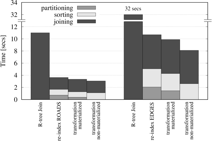
We then experiment with the three join strategies discussed in Section 5.2, starting with the setting where both input datasets are indexed by a $\mathsf{2\mbox{-}layer}$ scheme. The granularity of each first layer grid is set according to our analysis in Section 6.1 as powers of 2 (see Table V). We consider again the ROADS $\bowtie$ ZCTA5 and EDGES $\bowtie$ ZCTA5 queries.

Figure 12 reports the time breakdown of the tested approaches; as a baseline, we also included a traditional R-tree join method [37]. We tested the straightforward approach of re-indexing one of the inputs using a temporary $\mathsf{2\mbox{-}layer}$ so that both indices employ identical grids and being able to use the mj, all opts join method from the previous section. The figure shows the results for re-indexing ROADS and EDGES, while re-indexing ZCTA5 is omitted. As ZCTA5 contains significantly larger rectangles than ROADS and EDGES (see Table II), indexing these rectangles under the very fine grids used by $\mathsf{2\mbox{-}layer}$ for ROADS and EDGES incurs a high replication ratio and hence, high partitioning costs (over 300 secs). The figure also includes the two variants for the online transformation of the $\mathsf{2\mbox{-}layer}$ scheme in ROADS and EDGES to the grid of ZCTA5, proposed in Section 5.2.1. The results clearly show the benefit the online transformation compared to re-indexing one of the inputs and in particular, the variant when the new $\mathsf{2\mbox{-}layer}$ scheme is not materialized as such an approach completely eliminates the partitioning costs.

6.4.3 One Input Indexed

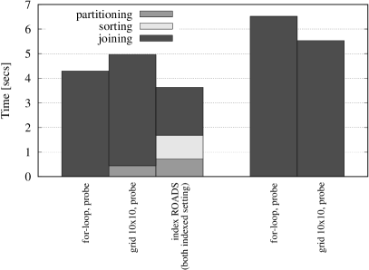
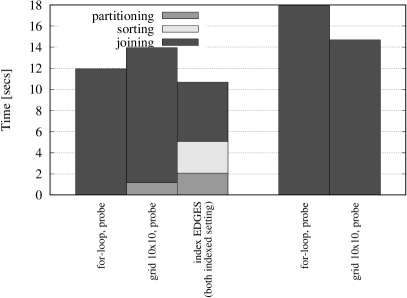
We consider once again the ROADS $\bowtie$ ZCTA5 and EDGES $\bowtie$ ZCTA5 queries when only one input is indexed by our $\mathsf{2\mbox{-}layer}$ scheme. We tested three solutions in this context. The first is a classic index-based join; we denote this approach as for-loop, probe. The second approach grid $10\times 10$, probe extends this idea by partitioning the unindexed input with a coarse grid (we used a $10\times 10$ one) and then executing the window range queries per grid cell. Finally, we also employed the ‘Both Inputs Indexed’ approach by indexing the unindexed input online.

Figure 13 reports the breakdown of the execution time; we distinguish between two cases for each query, depending on which input is already indexed. Note that we omit the ‘Both Inputs Indexed’ approach when ZCTA5 has to be indexed, similarly to previous section. We discuss the ROADS $\bowtie$ ZCTA5 query as the findings are the same for EDGES $\bowtie$ ZCTA5. When ZCTA5 is indexed, we observe that building online a temporary $\mathsf{2\mbox{-}layer}$ scheme on ROADS with an identical grid to ZCTA5 is in fact the best solution. This is mainly because mj, all opts used to compute the join drastically reduces the joining time. In contrast, when ROADS is pre-indexed, the best approach is grid $10\times 10$, probe which improves the cache locality when probing the index on ROADS. As ZCTA5 contains significantly fewer rectangles than ROAD, the cost of constructing such a grid is negligible compared to applying the same idea on ROADS when ZCTA5 is pre-indexed. To sum up, when one of the inputs is pre-indexed by our $\mathsf{2\mbox{-}layer}$ scheme, an $R\bowtie S$ spatial join can be efficiently computed using the ‘Both Inputs Indexed’ strategy if the cost of indexing the second input is expected to be low (due to containing small rectangles or using a coarse first layer grid) or the grid-based probe approach otherwise.

ROADS $\bowtie$ ZCTA5	EDGES $\bowtie$ ZCTA5

Figure 12: ‘Both Inputs Indexed’ setting on real datasets; re-indexing ZCTA5 omitted due to high online partitioning costs.

ROADS $\bowtie$ ZCTA5	EDGES $\bowtie$ ZCTA5
ZCTA5 indexed     ROADS indexed	ZCTA5 indexed     EDGES indexed

Figure 13: ‘One Input Indexed’ setting on real datasets; indexing ZCTA5 omitted due to high online partitioning costs.

6.4.4 No Input Indexed

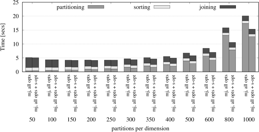
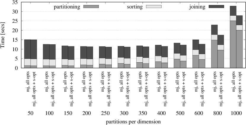
Lastly, we consider the setting when none of the inputs is indexed. As discussed in Section 5.2.3, we directly construct in this case, two temporary $\mathsf{2\mbox{-}layer}$ schemes under an identical first layer grid and then use mj, all opts to compute the join. Figure 14 shows the effect of further optimizing this approach with the space reduction optimization proposed at the end of Section 5.2.3, while varying the grid granularity. We denote this method as mj, all opts + s-opt. We observe that the space optimization enhances the join computation, especially when a very fine grid is used.

ROADS $\bowtie$ ZCTA5

EDGES $\bowtie$ ZCTA5

Figure 14: ‘No Input Indexed’ setting on real datasets

7 Conclusions

We presented a secondary partitioning approach that can be applied to SOP indices, such as grids, and divides the MBRs within each spatial partition to four classes. Our approach reduces the number of comparisons during range query evaluation and avoids the generation (and elimination) of duplicate results. We show how our approach can also be used for duplicate result avoidance in spatial intersection joins that are evaluated using the state-of-the-art PBSM algorithm. For both range queries and joins, we show how redundant computations can also be avoided. Our experimental findings confirm the superiority of our approach compared to the state-of-the-art duplicate result elimination method [18]. We also show that a grid equipped with our method outperforms other indices (such as the $\mathsf{quad\mbox{-}tree}$ and $\mathsf{R\mbox{-}tree}$) by up to one order of magnitude. The cost of spatial intersection joins is also reduced by a significant factor (about 50%) with the help of our secondary partitioning technique and the use of our optimized partition-to-partition join algorithms. Directions for future work include the evaluation of distance-based queries, e.g., $k$-NN or distance joins, the application of our approach to distributed spatial data management systems and to indexing trajectories for retrieval and join problems.

References

- [1] N. Mamoulis, Spatial Data Management, ser. Synthesis Lectures on Data Management. Morgan & Claypool Publishers, 2011.
- [2] A. Aji, F. Wang, H. Vo, R. Lee, Q. Liu, X. Zhang, and J. H. Saltz, “Hadoop-GIS: A high performance spatial data warehousing system over mapreduce,” Proc. VLDB Endow., vol. 6, no. 11, pp. 1009–1020, 2013.
- [3] A. Eldawy and M. F. Mokbel, “SpatialHadoop: A mapreduce framework for spatial data,” in IEEE ICDE, 2015, pp. 1352–1363.
- [4] D. Xie, F. Li, B. Yao, G. Li, L. Zhou, and M. Guo, “Simba: Efficient in-memory spatial analytics,” in ACM SIGMOD, 2016, pp. 1071–1085.
- [5] J. Yu, Z. Zhang, and M. Sarwat, “Spatial data management in apache spark: the geospark perspective and beyond,” GeoInformatica, vol. 23, no. 1, pp. 37–78, 2019.
- [6] V. Pandey, A. Kipf, T. Neumann, and A. Kemper, “How good are modern spatial analytics systems?” Proc. VLDB Endow., vol. 11, no. 11, pp. 1661–1673, 2018.
- [7] H. Hoppe, “Progressive meshes,” in ACM SIGGRAPH, 1996, pp. 99–108.
- [8] M. Pavlovic, D. Sidlauskas, T. Heinis, and A. Ailamaki, “QUASII: query-aware spatial incremental index,” in EDBT, 2018, pp. 325–336.
- [9] C. Cheng, H. Yang, I. King, and M. R. Lyu, “Fused matrix factorization with geographical and social influence in location-based social networks,” in AAAI, 2012.
- [10] A. Guttman, “R-trees: A dynamic index structure for spatial searching,” in ACM SIGMOD, 1984, pp. 47–57.
- [11] M. F. Mokbel, X. Xiong, and W. G. Aref, “SINA: scalable incremental processing of continuous queries in spatio-temporal databases,” in ACM SIGMOD, 2004, pp. 623–634.
- [12] D. V. Kalashnikov, S. Prabhakar, and S. E. Hambrusch, “Main memory evaluation of monitoring queries over moving objects,” Distributed and Parallel Databases, vol. 15, no. 2, pp. 117–135, 2004.
- [13] X. Yu, K. Q. Pu, and N. Koudas, “Monitoring k-nearest neighbor queries over moving objects,” in IEEE ICDE, 2005, pp. 631–642.
- [14] K. Mouratidis, M. Hadjieleftheriou, and D. Papadias, “Conceptual partitioning: An efficient method for continuous nearest neighbor monitoring,” in ACM SIGMOD, 2005, pp. 634–645.
- [15] D. Sidlauskas, S. Saltenis, C. W. Christiansen, J. M. Johansen, and D. Saulys, “Trees or grids?: indexing moving objects in main memory,” in ACM SIGSPATIAL/GIS, 2009, pp. 236–245.
- [16] S. Ray, R. Blanco, and A. K. Goel, “Supporting location-based services in a main-memory database,” in IEEE MDM, 2014, pp. 3–12.
- [17] W. G. Aref and H. Samet, “Hashing by proximity to process duplicates in spatial databases,” in CIKM, 1994, pp. 347–354.
- [18] J. Dittrich and B. Seeger, “Data redundancy and duplicate detection in spatial join processing,” in IEEE ICDE, 2000, pp. 535–546.
- [19] D. Tsitsigkos, K. Lampropoulos, P. Bouros, N. Mamoulis, and M. Terrovitis, “A two-layer partitioning for non-point spatial data,” in IEEE ICDE, 2021, pp. 1787–1798.
- [20] M. Olma, F. Tauheed, T. Heinis, and A. Ailamaki, “BLOCK: efficient execution of spatial range queries in main-memory,” in SSDBM, 2017, pp. 15:1–15:12.
- [21] J. L. Bentley and J. H. Friedman, “Data structures for range searching,” ACM Comput. Surv., vol. 11, no. 4, pp. 397–409, 1979.
- [22] J. L. Bentley, “Multidimensional binary search trees used for associative searching,” Commun. ACM, vol. 18, no. 9, pp. 509–517, 1975.
- [23] R. A. Finkel and J. L. Bentley, “Quad trees: A data structure for retrieval on composite keys,” Acta Inf., vol. 4, pp. 1–9, 1974.
- [24] M. T. Mahin, T. Hashem, and S. Kabir, “A crowd enabled approach for processing nearest neighbor and range queries in incomplete databases with accuracy guarantee,” Pervasive Mob. Comput., vol. 39, pp. 249–266, 2017.
- [25] H. Samet, The Design and Analysis of Spatial Data Structures. Addison-Wesley, 1990.
- [26] N. Beckmann, H. Kriegel, R. Schneider, and B. Seeger, “The R*-tree: An efficient and robust access method for points and rectangles,” in ACM SIGMOD, 1990, pp. 322–331.
- [27] K. Kim, S. K. Cha, and K. Kwon, “Optimizing multidimensional index trees for main memory access,” in ACM SIGMOD, 2001, pp. 139–150.
- [28] T. Vu and A. Eldawy, “R*-grove: Balanced spatial partitioning for large-scale datasets,” Frontiers Big Data, vol. 3, p. 28, 2020.
- [29] T. Kraska, A. Beutel, E. H. Chi, J. Dean, and N. Polyzotis, “The case for learned index structures,” in ACM SIGMOD, 2018, pp. 489–504.
- [30] H. Wang, X. Fu, J. Xu, and H. Lu, “Learned index for spatial queries,” in IEEE MDM, 2019, pp. 569–574.
- [31] P. Li, H. Lu, Q. Zheng, L. Yang, and G. Pan, “LISA: A learned index structure for spatial data,” in ACM SIGMOD, 2020, pp. 2119–2133.
- [32] J. Qi, G. Liu, C. S. Jensen, and L. Kulik, “Effectively learning spatial indices,” Proc. VLDB Endow., vol. 13, no. 11, pp. 2341–2354, 2020.
- [33] V. Nathan, J. Ding, M. Alizadeh, and T. Kraska, “Learning multi-dimensional indexes,” in ACM SIGMOD, 2020, pp. 985–1000.
- [34] J. Ding, V. Nathan, M. Alizadeh, and T. Kraska, “Tsunami: A learned multi-dimensional index for correlated data and skewed workloads,” Proc. VLDB Endow., vol. 14, no. 2, pp. 74–86, 2020.
- [35] F. P. Preparata and M. I. Shamos, Computational Geometry - An Introduction. Springer, 1985.
- [36] L. Arge, O. Procopiuc, S. Ramaswamy, T. Suel, and J. S. Vitter, “Scalable sweeping-based spatial join,” in VLDB, 1998, pp. 570–581.
- [37] T. Brinkhoff, H.-P. Kriegel, and B. Seeger, “Efficient processing of spatial joins using r-trees,” in ACM SIGMOD, 1993, pp. 237–246.
- [38] J. M. Patel and D. J. DeWitt, “Partition based spatial-merge join,” in ACM SIGMOD, 1996, pp. 259–270.
- [39] S. Nobari, Q. Qu, and C. S. Jensen, “In-memory spatial join: The data matters!” in EDBT, 2017, pp. 462–465.
- [40] D. Tsitsigkos, P. Bouros, N. Mamoulis, and M. Terrovitis, “Parallel in-memory evaluation of spatial joins,” in ACM SIGSPATIAL, 2019, pp. 516–519.
- [41] M.-L. Lo and C. V. Ravishankar, “Spatial hash-joins,” in ACM SIGMOD, 1996, pp. 247–258.
- [42] S. Nobari, F. Tauheed, T. Heinis, P. Karras, S. Bressan, and A. Ailamaki, “TOUCH: in-memory spatial join by hierarchical data-oriented partitioning,” in ACM SIGMOD, 2013, pp. 701–712.
- [43] S. T. Leutenegger, J. M. Edgington, and M. A. López, “STR: A simple and efficient algorithm for r-tree packing,” in IEEE ICDE, 1997, pp. 497–506.
- [44] N. Mamoulis and D. Papadias, “Slot index spatial join,” IEEE TKDE, vol. 15, no. 1, pp. 211–231, 2003.
- [45] F. Tauheed, T. Heinis, and A. Ailamaki, “Configuring spatial grids for efficient main memory joins,” in BICOD, 2015.
- [46] A. Cary, Z. Sun, V. Hristidis, and N. Rishe, “Experiences on processing spatial data with mapreduce,” in SSDBM, 2009, pp. 302–319.
- [47] S. You, J. Zhang, and L. Gruenwald, “Large-scale spatial join query processing in cloud,” in CloudDB, ICDE Workshops, 2015, pp. 34–41.
- [48] A. Eldawy, V. Hristidis, S. Ghosh, M. Saeedan, A. Sevim, A. B. Siddique, S. Singla, G. Sivaram, T. Vu, and Y. Zhang, “Beast: Scalable exploratory analytics on spatio-temporal data,” in ACM CIKM, 2021, pp. 3796–3807.
- [49] I. Sabek and M. F. Mokbel, “On spatial joins in mapreduce,” in ACM SIGSPATIAL, 2017, pp. 21:1–21:10.
- [50] G. Kedem, “The quad-cif tree: A data structure for hierarchical on-line algorithms,” in DAC, 1982, pp. 352–357.
- [51] M. Loskot and A. Wulkiewicz, 2019, https://github.com/mloskot/spatial_index_benchmark.