PAC Neural Prediction Set Learning to Quantify the Uncertainty of Generative Language Models

Abstract

Uncertainty learning and quantification of models are crucial tasks to enhance the trustworthiness of the models. Importantly, the recent surge of generative language models (GLMs) emphasizes the need for reliable uncertainty quantification due to the concerns on generating hallucinated facts. In this paper, we propose to learn neural prediction set models that comes with the probably approximately correct (PAC) guarantee for quantifying the uncertainty of GLMs. Unlike existing prediction set models, which are parameterized by a scalar value, we propose to parameterize prediction sets via neural networks, which achieves more precise uncertainty quantification but still satisfies the PAC guarantee. We demonstrate the efficacy of our method on four types of language datasets and six types of models by showing that our method improves the quantified uncertainty by $63\%$ on average, compared to a standard baseline method.

1 Introduction

Generative language models (GLMs) [31, 6, 36, 35] have achieved great attention in their abilities of generating human-level languages [22] mainly due to transformer architectures [38]. However, GLMs raise concerns on generating hallucinated facts [17], an unwilling property of GLMs as knowledge retrieval bases. This property can be suppressed by fine-tuning [17, 23] via feeding human-curated data, which is expensive in training and labeling cost. Instead, we leverage uncertainty quantification to alarm the uncertain or provably-wrong responses of GLMs to end-users, without updating GLMs.

Uncertainty quantification aims to measure the uncertainty of model predictions, and conformal prediction [40] is a promising way for quantifying uncertainty as it provides correctness guarantees with finite samples under minimal assumptions. In particular, the goal of conformal prediction is to construct prediction sets on predictions by a given model, where the prediction set is a set of labels that possibly contains a true label of a given example. Here, the prediction set size quantifies the uncertainty of a prediction by the given model (e.g., if the given model is uncertain on a label prediction, the corresponding prediction set is large, providing multiple label choices in classification).

In this paper, we propose to quantify the uncertainty of GLMs via conformal prediction. To this end, we first propose a novel prediction set representation, inspired by the learning theoretic interpretation of conformal prediction [26]. In particular, a prediction set in conformal prediction is parameterized via a scalar variable [24, 26]. This parameterization has shown its efficacy in many practical tasks, including classification and regression [24, 40, 26, 1, 4, 25]. However, we claim that the scalar-parameterized prediction set (SPS) is insufficient to capture better uncertainty in GLMs. Specifically, we wish to mitigate the issue on hallucinated facts of GLMs by providing uncertainty via a prediction set for each token (i.e., token-wise uncertainty) to highlight uncertain tokens in a generated response. To this end, a prediction set of each token needs to exploit the context of the token, provided by the previous tokens, to have more precise uncertainty. But, the scalar parameter cannot encode the context due to its independence on tokens. To address this issue, we consider the high-dimensional representation of the prediction set by parameterizing it via a neural network output given tokens, called a neural prediction set (NPS). See Section 3.2 for details.

Along with the new representation of prediction sets, we provide a PAC learning algorithm to learn a neural prediction set model. In particular, PAC learning algorithm prefers to be sample-efficient, but the practical sample-complexity bound of neural networks exist only in limited setups [3, 7, 2]. We exploit the structural properties of the family of neural prediction sets to devise a sample-efficient PAC learning algorithm (see Section 3.3 for details).

Finally, we demonstrate the efficacy of our method by using four types of natural language datasets [5, 33, 44, 8, 15, 32, 34] and the six types of GLMs [31, 36, 35], and by showing that our method satisfies the PAC guarantee, while producing $63\%$ smaller prediction set size (i.e., significantly better uncertainty quantifier), compared to a baseline method. See Figure 1 for the examples of token-wise uncertainty quantification.

Question	The city of Geneva is in which European country?
SPS	Switzerland.
NPS (ours)	Switzerland.

(a) More-certain. The GLM generates a right answer (i.e., “Switzerland”). NPS quantifies that there are not many alternatives than “Switzerland”.

Question	Name the British scientist who shared the 2013 Nobel Prize for Physics.
SPS	The British scientist who shared the 2013 Nobel Prize for Physics is James Peebles, Michel Mayor and Didier Queloz.
NPS (ours)	The British scientist who shared the 2013 Nobel Prize for Physics is James Peebles, Michel Mayor and Didier Queloz.

(b) Less-certain. The GLM generates the names of three scientists, who are not British. NPS quantifies that there are a few alternatives than the three names.

Question	Who was the last British winner of the Nobel Prize for Literature?
SPS	The last British winner of the Nobel Prize for Literature was artist Bob Dylan in 2016.
NPS (ours)	The last British winner of the Nobel Prize for Literature was artist Bob Dylan in 2016.

(c) Provably-uncertain. The GLM generates a wrong answer (i.e., “Bob Dylan” was the winner of the Nobel Prize for Literature but is not British). NPS confirms that “artist Bob Dylan in 2016” is not a right answer with high probability due to the PAC guarantee.

Figure 1: The proposed method NPS reasonably quantifies the token-wise uncertainty of the answers of the Alpaca-7B model [35] on questions from TriviaQA [15] with the PAC guarantee, while SPS is uncertain for most tokens. Here, the uncertainty is represented in the intensity of the “red” background color, which is proportional to the number of alternative tokens.

1.1 Related Work

We introduce related work on uncertainty quantification and its application to GLMs.

Calibration in GLMs. Calibration is one technique to quantify the uncertainty of predicted labels, which goal is predicting the correctness of a given prediction, also called confidence. Calibration is historically explored in forecasting and statistical machine learning [21, 30, 42, 43, 13, 29], where modern neural networks have been empirically identified their overconfidence [13].

In neural language generation, GLMs for question-answering are also demonstrated to be poorly calibrated, and conventional calibration methods (e.g., temperature scaling [30, 13]) partially contribute to address the mis-calibration issue of GLMs [14]. Contrast to the conventional calibration methods (also called probabilistic calibration), the concept of “linguistic calibration” (i.e., generating an answer with a verbalized expression of confidence) is proposed and its effectiveness within generative dialog agents is demonstrated [19]. The aforementioned calibration methods for GLMs are empirically effective but do not provide the correctness guarantee with finite samples as a basis of trust on quantified uncertainty, while we rely on conformal prediction to quantify uncertainty that comes with correctness guarantees with finite samples.

Conformal prediction. The goal of conformal prediction [40] is to construct a prediction set that likely contains true label, where the set size represents uncertainty. Depending on the problem setups, there are many ways to define and enforce the correctness guarantee in conformal prediction: classification or regression [40, 39, 4], meta learning [10, 27], and online learning [12]. Recently, PAC prediction sets [26] are used to construct prediction sets over partial programs, generated by GLMs of code [16]. One distinguishing feature of conformal prediction is that a prediction set is parameterized in a scalar variable [24, 26, 4], which implies that the scalar parameter is the same regardless of input examples. However, this produces conservative prediction sets in sequential prediction problems. In particular, in language generation, a sequence of prediction sets is generated for each token given a prompt, where each token has a different-level of uncertainty while conformal prediction uses the same scalar parameter for all prediction sets of each token to measure uncertainty; thus, this “coarse” prediction sets tend to be larger. We overcome this issue by considering a high-dimensional parameter via neural networks.

2 PAC Prediction Set Learning for GLMs

We consider the problem of learning prediction sets for GLMs. Here, we first provide preliminaries on the problem, followed by our problem statement.

2.1 Background: Conformal Prediction and PAC Prediction Sets

Conformal prediction [40] provides a promising way to quantify uncertainty with a correctness guarantee under minimal assumptions. Here, we consider PAC prediction sets [26], an interpretation of tolerance region [41] and training-conditional inductive conformal prediction [39] in the lens of PAC learning theory [37] (i.e., learning a “good” function within a function family from data). This interpretation inspires us to generalize conformal prediction for GLMs.

Prediction Set Models. Let $\mathcal{{X}}$ be an example space, $\mathcal{{Y}}$ be a label space, and $D$ be a distribution over $\mathcal{{X}}\times\mathcal{{Y}}$. We consider a (conformal) prediction set model $\hat{{C}}:\mathcal{{X}}\to 2^{\mathcal{{Y}}}$ with a scalar parameter [24, 26] as follows:

$$C(x)\coloneqq\left\{y\in\mathcal{{Y}}\mid f(x,y)\geq\tau\right\},$$ (1)

where $f:\mathcal{{X}}\times\mathcal{{Y}}\to\mathbb{R}_{\geq 0}$ is a (conformal) scoring function that measures the conformity (or likelihood) of $x$ for being $y$ with respect to $f$ (thus, we call $f(x,y)$ a conformity score), and $\tau\in\mathbb{R}_{\geq 0}$ is a scalar parameter. We denote the family of all prediction sets with a scalar parameter by $\mathcal{{T}}$.

Prediction set and its size. The output of the prediction set model is a set of possible label predictions, constructed to likely include a future label; thus, it is called a prediction set. Here, the size of a prediction set $|C(x)|$ measures the uncertainty of $f$ on $x$, i.e., if the prediction set size is large (or small), $f$ is uncertain (or certain) on the label prediction of $x$.

From (1), the size is determined by the parameter $\tau$ given $f$, so we maximize $\tau$ to closely measure the uncertainty of $f$, while maintaining that the prediction set $C(x)$ mostly contains the true label of $x$ (i.e., learning a “correct” $C$). To this end, we consider the definition of correctness along with a necessary assumption in the following.

Assumption. We assume that samples are independent and identically distributed (i.i.d.) (i.e., the i.i.d. assumption) in this paper. In particular, all samples for testing and learning prediction sets are independently drawn from the same but known distribution $D$.

PAC guarantee. Under the i.i.d. assumption, we learn a prediction set $\hat{{C}}$ that includes the most true labels (approximately correct), i.e., the expected error of $\hat{{C}}$ is less than a desired error level $\varepsilon\in(0,1)$

$$L(\hat{{C}})\coloneqq\mathbbm{P}\Big{\{}y\notin\hat{{C}}(x)\Big{\}}\leq\varepsilon,$$

where the probability is taken over i.i.d. samples $(x,y)\sim D$. Here, the prediction set $\hat{{C}}$ is learned from a calibration set, so we desire to construct $\hat{{C}}$ that has a desired error most of the time (probably approximately correct), i.e.,

$$\mathbbm{P}\Big{\{}\mathbbm{P}\Big{\{}y\notin\hat{{C}}(x)\Big{\}}\leq\varepsilon\Big{\}}\geq 1-\delta,$$ (2)

where $\delta\in(0,1)$ is a desired confidence level and the outer probability is taken over $n$ i.i.d. calibration samples $Z\sim D^{n}$, used to learn $\hat{{C}}$.

Algorithm. The PAC prediction set approach [26, 28] considers the following algorithm $\mathcal{{A}}_{\text{Binom}}:(\mathcal{{X}}\times\mathcal{{Y}})^{*}\to\mathcal{{T}}$ to learn a prediction set model $\hat{{C}}$, parameterized by $\hat{\tau}$:

$$\mathcal{{A}}_{\text{Binom}}:\qquad\hat{\tau}=\max_{\tau\in\mathbb{R}_{\geq 0}}~{}\tau\qquad\text{subj. to}\qquad U_{\text{Binom}}(C,Z,\delta)\leq\varepsilon,$$ (3)

where $C$ is parameterized by $\tau$, $\bar{L}_{n}(C)\!\coloneqq\!\sum_{i=1}^{n}\!\mathbbm{1}\left(y_{i}\!\notin\!C(x_{i})\right)$ is the empirical error count of $C$, $F(k;n,\theta)$ is a cumulative distribution function of a binomial distribution with $n$ trials and success probability $\theta$, and $U_{\text{Binom}}(C,Z,\delta)\!\coloneqq\!\inf\left\{\theta\in[0,1]\!\mid\!F(\bar{L}_{n}(C);n,\theta)\!\leq\!\delta\right\}\!\cup\!\{1\}$ is a binomial tail bound, i.e., $\mathbbm{P}\!\left\{L(C)\!\leq\!U_{\text{Binom}}(C,Z,\delta)\right\}\!\geq\!1-\delta$ for any $C$. This algorithm is PAC.

Theorem 1.

([39, 26, 28]) The algorithm $\mathcal{{A}}_{\text{Binom}}$ is PAC, i.e., for any $f$, $\varepsilon\in(0,1)$, $\delta\in(0,1)$, and $n\in\mathbb{Z}_{\geq 0}$, we have $\mathbbm{P}\{\mathbbm{P}\{y\notin\hat{{C}}(x)\}\leq\varepsilon\}\geq 1-\delta$, where the inner probability is taken over a labeled example $(x,y)\sim D$, the outer probability is taken over i.i.d. labeled examples $Z\sim D^{n}$, and $\hat{{C}}=\mathcal{{A}}_{\text{Binom}}(Z)$.

Note that the PAC guarantee generally holds only if an enough number of samples is provided (when we know a function family including a true function). However, we consider PAC algorithms that hold for any number of samples due to the structural property of prediction sets, i.e., a prediction set is always correct if $\tau=0$ (thus $\smash{\hat{{C}}}(x)=\mathcal{{Y}}$), regardless of the sample size. In other words, the calibration samples are not sufficient, the prediction set is constructed to return $\mathcal{{Y}}$ to satisfy the PAC guarantee. We include a proof in the following.

Proof.

Let $C_{\tau}$ be a prediction set $C$ with a parameter $\tau$, $\mathcal{{H}}_{\varepsilon}\coloneqq\left\{\tau\in\mathbb{R}_{\geq 0}\mid L(C_{\tau})>\varepsilon\right\}$, and $\tau^{*}\coloneqq\inf\mathcal{{H}}_{\varepsilon}$. Then, we have

$$\mathbbm{P}\Big{\{}L(\mathcal{{A}}_{\text{Binom}}(Z))>\varepsilon\Big{\}}\!=\!\mathbbm{P}\Big{\{}\exists{\tau\in\mathcal{{H}}_{\varepsilon}},U_{\text{Binom}}(C_{\tau},Z,\delta)\leq\varepsilon\Big{\}}\!=\!\mathbbm{P}\Big{\{}U_{\text{Binom}}(C_{\tau^{*}},Z,\delta)\leq\varepsilon\Big{\}}$$ (4)

$$=\mathbbm{P}\Big{\{}L(C_{\tau^{*}})>\varepsilon\wedge U_{\text{Binom}}(C_{\tau^{*}},Z,\delta)\leq\varepsilon\Big{\}}\leq\mathbbm{P}\Big{\{}L(C_{\tau^{*}})>U_{\text{Binom}}(C_{\tau^{*}},Z,\delta)\Big{\}}\leq\delta,$$ (5)

where the last equality in (4) holds as $\mathbbm{1}\left(y\notin C_{\tau}(x)\right)$ and $U_{\text{Binom}}$ are non-decreasing in $\tau$ (i.e., Lemma 2 in [28]) and the last inequality in (5) is due to the property of the binomial tail bound $U_{\text{Binom}}$. ∎

2.2 Problem Statement

Let $\mathcal{{X}}$ be a token space (e.g., a set of tokens in Byte Pair Encoding [11]). Then, we denote an example (or a prompt) by $\mathbf{x}\in\mathcal{{X}}^{*}$, a label (or a response) by $\mathbf{y}\in\mathcal{{X}}^{*}$, and a distribution over labeled examples $\mathcal{{X}}^{*}\times\mathcal{{X}}^{*}$ by $\mathbf{D}$, considering that each prompt has a desired response. Here, $\mathbf{x}$ (and also $\mathbf{y}$) is a sequence of tokens, i.e., $\mathbf{x}\coloneqq(\mathbf{x}_{1},\dots,\mathbf{x}_{l})$, so we denote its length by $|\mathbf{x}|$, i.e., $|\mathbf{x}|=l$, and a sub-sequence from the $i$-th token to the $j$-th token by $\mathbf{x}_{i:j}$.

Our goal is to find a PAC learning algorithm that returns a prediction set model given learning samples. In particular, under the i.i.d. assumption, for any $\varepsilon\in(0,1)$, $\delta\in(0,1)$, and $n\in\mathbb{Z}_{\geq 0}$, given a family of prediction sets $\mathcal{{F}}$, we find $\mathcal{{A}}:(\mathcal{{X}}^{*}\times\mathcal{{X}}^{*})^{*}\to\mathcal{{F}}$ that satisfies

$$\mathbbm{P}\left\{\mathbbm{P}\left\{\mathbf{y}\notin\hat{{C}}(\mathbf{x})\right\}\leq\varepsilon\right\}\geq 1-\delta,$$ (6)

where the inner probability is taken over an labeled example $(\mathbf{x},\mathbf{y})\sim\mathbf{D}$, the outer probability is taken over a calibration set $\mathbf{Z}\sim\mathbf{D}^{n}$, and $\mathcal{{A}}(\mathbf{Z})=\hat{{C}}$. Along with the PAC guarantee, we wish our algorithm achieving optimal prediction set size, i.e., minimizing $\mathbbm{E}\hat{{C}}(\mathbf{x})$, while satisfying (6).

3 Neural Prediction Set Models for GLMs

We discuss our proposed method in defining and learning neural prediction set models, along with an algorithm with the PAC guarantee. This section ends with the applications of neural prediction sets in the uncertainty quantification of GLMs.

3.1 Recursive Definition of Prediction Sets

We mainly use prediction sets to measure token-wise uncertainty by adopting the recursive definition of prediction sets. In particular, we define the $l$-th prediction set $C_{l}:\mathcal{{X}}^{*}\to 2^{\smash{\mathcal{{X}}}^{l}}$ as follows:

$$C_{l}(\mathbf{x})\coloneqq\Big{\{}(\mathbf{y},y)\in C_{l-1}(\mathbf{x})\times\mathcal{{X}}\;\Big{|}\;f((\mathbf{x},\mathbf{y}),y)\geq\tau\Big{\}},$$ (7)

where $C_{1}(\mathbf{x})=\left\{y\in\mathcal{{X}}\;\middle|\;f(\mathbf{x},y)\geq\tau\right\}$. Here, we consider a scoring function $f:\mathcal{{X}}^{*}\times\mathcal{{X}}\to\mathbb{R}_{\geq 0}$, which can be any generative language model (e.g., GPT-3 [6]). Note that the size of the prediction set (7) grows exponentially as $l$ grows, but we mainly consider conditional prediction sets, where the size only grows linearly (see Section 3.5 for details).

3.2 Example-dependent Parameterization

The recursive prediction set constructs a prediction set, conditioned on previous labels. However, the scalar parameter $\tau$ in (7) is used by all prediction sets, i.e., the parameter is example-agnostic, which mainly introduces conservative prediction set size especially for modeling the uncertainty of structured and sequential language generators.

Inspired from the learning theoretical interpretation of conformal prediction [26], we consider the conformal prediction in learning a prediction set among a richer family of prediction sets, parameterized via neural networks. In particular, we design the parameter of prediction sets as the output of any neural network $\tau:\mathcal{{X}}^{*}\to\mathbb{R}_{\geq 0}$, which depends on previous tokens, instead of a scalar parameter $\tau\in\mathbb{R}_{\geq 0}$, which is independent to previous tokens. Thus, our prediction set, parameterized via a neural network, is called a neural prediction set model and defined as follows:

$$C_{l}(\mathbf{x})\coloneqq\Big{\{}(\mathbf{y},y)\in C_{l-1}(\mathbf{x})\times\mathcal{{X}}\;\Big{|}\;f((\mathbf{x},\mathbf{y}),y)\geq\tau(\mathbf{x},\mathbf{y})\Big{\}},$$ (8)

where $C_{1}(\mathbf{x})=\left\{y\in\mathcal{{X}}\;\middle|\;f(\mathbf{x},y)\geq\tau(\mathbf{x})\right\}$. Here, we denote the family of all neural prediction set models by $\mathcal{{F}}\coloneqq\{C_{l}:\mathcal{{X}}^{*}\to 2^{\mathcal{{X}}^{l}}\mid l\geq 1,\tau\in\mathcal{{F}}^{\prime}\}$, where $\mathcal{{F}}^{\prime}$ is any family of neural networks.

3.3 Decomposition for a Sample-Efficient PAC Algorithm

Given a family of neural prediction set models $\mathcal{{F}}$, finding a PAC algorithm requires a sample-complexity analysis, i.e., finding a minimal number of samples such that the algorithm chooses a function in $\mathcal{{F}}$ with a desired expected error rate with high probability. However, it is generally known that the existing sample-complexity bounds of neural networks are yet to be practical, e.g., the data-independent VC dimension bound is too pessimistic or the width of neural networks should be $\Omega(n^{7})$ (where $n$ is the number of samples) to have a tighter data-dependent bound than the VC bound [9, 7, 2].

(a) Scalar prediction set

(b) Neural prediction set

Figure 2: The shape of $\tau$. (2(a)) The restrictive $\tau$ introduces gaps between $\tau$ and conformity scores $f(\mathbf{x},y)$, constructing larger prediction sets. (2(b)) The ideal shape of $\tau(\mathbf{x})$ forms a tight “hammock” to support conformity scores $f(\mathbf{x},y)$ in neural prediction sets, implying that the set size is small, i.e., the gaps between $\tau(\mathbf{x})$ and $f(\mathbf{x},y)$ are small.

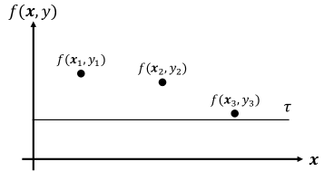
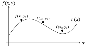
To avoid the high sample-complexity issue, we exploit a structural property of the family of neural prediction sets $\mathcal{{F}}$. In particular, we observe that the ideal shape of $\tau(\mathbf{x})$ forms a “hammock” to “vertically” support conformity scores $f(\mathbf{x},y)$, as illustrated in Figure 2(b). This observation provides us that if the “shape” of “hammock” is fixed, “vertically translating” the “hammock” can control a desired expected error rate at any level. In this way, we can reduce the search space of $\mathcal{{F}}$, leading to a significantly lower sample-complexity bound. We concretize this idea in the following section.

Decomposition. We consider the following decomposition of a neural prediction set parameter $\tau(\mathbf{x})$:

$$\log\tau(\mathbf{x})\coloneqq g(\mathbf{x})+h,$$ (9)

where $g:\mathcal{{X}}^{*}\to\mathbb{R}$ is a neural network, and $h\in\mathbb{R}$ is a scalar parameter. Here, we denote a set of all $g$ and $h$ by $\mathcal{{G}}^{\prime}$ and $\mathcal{{H}}^{\prime}$, respectively.

Structural Property. Each component of the decomposed parameter in (9) has its own property. In particular, $g$ and $h$ mainly control the size and error of prediction sets, respectively, which is evident if we consider the following reformulation of the scoring function and parameters:

$$f(\mathbf{x},y)\geq\tau(\mathbf{x})\Longleftrightarrow\frac{f(\mathbf{x},y)}{\exp{g(\mathbf{x})}}\geq\exp{h}.$$ (10)

Here, $g(\mathbf{x})$ contributes to rescaling the scoring function and $\exp{h}$ controls the prediction set error given a scoring function, as the scalar-parameterized prediction sets in Section 2.1.

Learning $h$. Given $g$, learning $h$ is equivalent to learning prediction sets with a scalar parameter (3); we denote the following algorithm to learn $h$ by $\mathcal{{A}}_{h}:\mathcal{{G}}^{\prime}\times(\mathcal{{X}}^{*}\times\mathcal{{X}}^{*})^{*}\to\mathcal{{F}}$.

$$\mathcal{{A}}_{h}(g,\mathbf{Z}_{h}): \quad\hat{{h}}=\arg\max_{h\in\mathbb{R}}~{}h\qquad\text{subj. to}\qquad U_{\text{Binom}}(\exp{h},\mathbf{Z}_{h},\delta)\leq\varepsilon,$$

where $\mathbf{Z}_{h}$ is the calibration set to learn $h$. Here, the error of a neural prediction set model on a single example is simplified as $\mathbbm{1}\left(\mathbf{y}\notin C_{|\mathbf{y}|}(\mathbf{x})\right)=\bigvee_{l=1}^{|\mathbf{y}|}f((\mathbf{x},\mathbf{y}_{1:l-1}),\mathbf{y}_{l})<\tau(\mathbf{x},\mathbf{y}_{1:l-1}),$ which is monotonically non-decreasing in $h$, so minimizing this error maximizes the expected size [28].

As the PAC guarantee in Theorem 1 holds for any scoring function, due to the scoring-function reformulation in (10), we have the following PAC guarantee. Appendix A for a proof.

Lemma 1.

For any $g\in\mathcal{{G}}^{\prime}$, $\mathcal{{A}}_{h}$ is $(\varepsilon,\delta)$-PAC.

Learning $g$. The neural network $g$ captures the trend of conformity scores over data. To learn $g$, any algorithm is fine as the PAC guarantee holds (as in Lemma 1) regardless of the learning algorithm. However, $g$ that closely follows the conformity scores of data provides a good uncertainty quantifier in terms of prediction set size. In particular, given $(\mathbf{x},y)$, $\tau^{*}(\mathbf{x})=f(\mathbf{x},y)$ is the optimal $\tau$ in the prediction set size. To learn the optimal $\tau^{*}$, we consider the learning problem of $g$ as regression over the conformity scores, i.e., finding $g$ that minimizes the absolute error between $f$ and $g$. In particular, we consider the algorithm $\mathcal{{A}}_{g}:(\mathcal{{X}}^{*}\times\mathcal{{X}}^{*})^{*}\to\mathcal{{G}}^{\prime}$ that solves the following standard regression problem, given a hold-out set $\mathbf{Z}_{g}$:

$$\mathcal{{A}}_{g}(\mathbf{Z}_{g}): \quad\hat{{g}}=\arg\min_{g\in\mathcal{{G}}^{\prime}}~{}\frac{1}{|\mathbf{Z}^{\prime}_{g}|}\sum_{(\mathbf{x},\mathbf{y})\in\mathbf{Z}^{\prime}_{g}}\frac{1}{|\mathbf{y}|}\sum_{l=1}^{|\mathbf{y}|}\left|\log f((\mathbf{x},\mathbf{y}_{1:l-1}),\mathbf{y}_{l})-\log g(\mathbf{x},\mathbf{y}_{1:l-1})\right|,$$ (11)

Here, $\mathbf{Z}^{\prime}_{g}$ and $\mathbf{Z}^{\prime\prime}_{g}$ are randomly partitioned from $\mathbf{Z}_{g}$, i.e., $\mathbf{Z}_{g}=\mathbf{Z}^{\prime}_{g}\cup\mathbf{Z}^{\prime\prime}_{g}$ and $\emptyset=\mathbf{Z}^{\prime}_{g}\cap\mathbf{Z}^{\prime\prime}_{g}$, where $\mathbf{Z}^{\prime\prime}_{g}$ is used to choose the best $g$.

Design choice of $g$. The neural network $g:\mathcal{{X}}^{*}\to\mathbb{R}$ is part of the parameters of neural prediction set models. Here, we exploit a hidden state of a GLM given an input prompt $\mathbf{x}$. In particular, letting $\mathcal{{H}}$ be an embedding space of a given GLM, formed by an embedding $g_{1}:\mathcal{{X}}^{*}\to\mathcal{{H}}$, and $g_{2}:\mathcal{{H}}\to\mathbb{R}$ be a neural network, we choose $g:\mathbf{x}\mapsto g_{2}(g_{1}(\mathbf{x}))$, and learn $g_{2}$ in $\mathcal{{A}}_{g}$ of (11), while fixing $g_{1}$.

Algorithm $\mathcal{{A}}_{\text{NPS}}$. The final algorithm, called $\mathcal{{A}}_{\text{NPS}}$, is the composition of $\mathcal{{A}}_{g}$ and $\mathcal{{A}}_{h}$, i.e., $\mathcal{{A}}_{\text{NPS}}:\mathbf{Z}\mapsto\mathcal{{A}}_{h}(\mathcal{{A}}_{g}(\mathbf{Z}_{g}),\mathbf{Z}_{h})$, where $\mathbf{Z}$ is randomly partitioned into $\mathbf{Z}_{g}$ and $\mathbf{Z}_{h}$, i.e., $\mathbf{Z}=\mathbf{Z}_{g}\cup\mathbf{Z}_{h}$ and $\emptyset=\mathbf{Z}_{g}\cap\mathbf{Z}_{h}$. Here, we assume $|\mathbf{Z}_{g}|=|\mathbf{Z}_{h}|$. Interestingly, our algorithm has better sample-complexity to achieve the PAC guarantee with smaller set size, compared to the baseline PAC prediction set algorithm (3). In particular, even though we hold out the half of a calibration set for the heuristic learning of $g$ and use only half of the set for PAC learning, our algorithm achieves clearly smaller prediction set size, on average, than the baseline algorithm with a full calibration set. See Section 4 for empirical results.

3.4 PAC Guarantee

We prove that the proposed algorithm $\mathcal{{A}}_{\text{NPS}}$ is PAC. This is the direct consequence of Lemma 1.

Theorem 2.

The algorithm $\mathcal{{A}}_{\text{NPS}}$ is PAC, i.e., for any $f$, $\varepsilon\in(0,1)$, $\delta\in(0,1)$, and $n\in\mathbb{Z}_{\geq 0}$, we have $\mathbbm{P}\{\mathbbm{P}\{\mathbf{y}\notin\hat{{C}}(\mathbf{x})\}\leq\varepsilon\}\geq 1-\delta$, where the inner probability is taken over a labeled example $(\mathbf{x},\mathbf{y})\sim\mathbf{D}$, the outer probability is taken over i.i.d. labeled examples $\mathbf{Z}\sim\mathbf{D}^{n}$, and $\hat{{C}}=\mathcal{{A}}_{\text{NPS}}(\mathbf{Z})$.

Proof.

From Lemma 1, for any $g$, including the output of $\mathcal{{A}}_{g}$, $\mathcal{{A}}_{h}$ is $(\varepsilon,\delta)$-PAC. As $\mathcal{{A}}_{g}$ and $\mathcal{{A}}_{h}$ use non-overlapping labeled examples and $\mathcal{{A}}_{h}$ is $(\varepsilon,\delta)$-PAC, so $\mathcal{{A}}_{\text{NPS}}$ does. ∎

3.5 Applications to Uncertainty Quantification of GLMs

The neural prediction sets constructed by the PAC algorithm can be used as the basis of the trust on the quantified uncertainty via the set size. Here, we mainly consider token-wise uncertainty.

Token-wise uncertainty. Suppose that we have $\hat{{C}}\in\mathcal{{F}}$ from our PAC algorithm $\mathcal{{A}}_{\text{NPS}}$, a prompt $\mathbf{x}$, and a generated token sequence $\mathbf{y}^{\prime}_{1:l-1}$ (from a GLM given $\mathbf{x}$); then we have the following conditional neural prediction set for the $l$-th token:

$$\hat{{C}}_{l}(\mathbf{x};\mathbf{y}^{\prime}_{1:l-1})=\begin{cases}\left\{y\in\mathcal{{X}}\;\middle|\;f((\mathbf{x},\mathbf{y}^{\prime}_{1:l-1}),y)\geq\hat{\tau}(\mathbf{x},\mathbf{y}^{\prime}_{1:l-1})\right\}&\text{if~{}$\mathbf{y}^{\prime}_{1:l-1}\in\hat{{C}}_{l-1}(\mathbf{x})$}\\ \mathcal{{X}}&\text{otherwise}\end{cases},$$ (12)

where $|\hat{{C}}_{l}(\mathbf{x};\mathbf{y}^{\prime}_{1:l-1})|$ represents the uncertainty of the $l$-th token prediction, i.e., the number of alternative tokens for the $l$-th token. Here, the uncertainty by the conditional prediction set is probably invalid if $\mathbf{y}^{\prime}_{1:l-1}\notin\hat{{C}}_{l-1}(\mathbf{x})$ but we cannot reject its validity otherwise. In particular, the provided PAC guarantee implies $\mathbbm{P}\{\mathbf{y}\in\hat{{C}}(\mathbf{x})\}\geq 1-\varepsilon$, meaning that a true response $\mathbf{y}$ is likely included in the prediction set $\hat{{C}}(\mathbf{x})$. Thus, if $\mathbf{y}^{\prime}_{1:l-1}\notin\hat{{C}}_{l-1}(\mathbf{x})$, the generated sub-sequence $\mathbf{y}^{\prime}_{1:l-1}$ is unlikely to be the sub-sequence of the true response $\mathbf{y}$. In this case, the prediction set returns the entire set $\mathcal{{X}}$ to indicate the probable invalidity of the generated subsequence. When $\mathbf{y}^{\prime}_{1:l-1}\in\hat{{C}}_{l-1}(\mathbf{x})$, we cannot reject the possibility that the generated sequence is the true sequence, so we still use the conditional prediction set $\hat{{C}}_{l}(\mathbf{x};\mathbf{y}^{\prime}_{1:l-1})$ to quantify the uncertainty of the $l$-th token, assuming $\mathbf{y}^{\prime}_{1:l-1}$ is part of the true response.

4 Experiments

Scoring function	Method	Datasets								Mean size
		Common sense reasoning		Closed-book QA		Open-book QA		Mathematical reasoning
		Error	Size${}_{\text{mean}}$ Size${}_{\text{median}}$	Error	Size${}_{\text{mean}}$ Size${}_{\text{median}}$	Error	Size${}_{\text{mean}}$ Size${}_{\text{median}}$	Error	Size${}_{\text{mean}}$ Size${}_{\text{median}}$
GPT-2 Small (120M)	SPS	0.0081 $\pm$ 0.0002	0.3012 $\pm$ 0.0041 0.2669 $\pm$ 0.0041	0.0086 $\pm$ 0.0001	0.2197 $\pm$ 0.0012 0.2049 $\pm$ 0.0012	0.0081 $\pm$ 0.0001	0.0747 $\pm$ 0.0008 0.0636 $\pm$ 0.0007	0.0091 $\pm$ 0.0003	0.1258 $\pm$ 0.0022 0.1171 $\pm$ 0.0021	0.1803 $\pm$ 0.0871 0.1632 $\pm$ 0.0784
	NPS (ours)	0.0078 $\pm$ 0.0006	0.2969 $\pm$ 0.0063 0.2399 $\pm$ 0.0077	0.0068 $\pm$ 0.0001	0.3297 $\pm$ 0.0041 0.2904 $\pm$ 0.0049	0.0078 $\pm$ 0.0005	0.0863 $\pm$ 0.0045 0.0423 $\pm$ 0.0037	0.0074 $\pm$ 0.0002	0.1764 $\pm$ 0.0066 0.1069 $\pm$ 0.0057	0.2223 $\pm$ 0.0972 0.1699 $\pm$ 0.0997
GPT-2 Medium (340M)	SPS	0.0086 $\pm$ 0.0002	0.2434 $\pm$ 0.0034 0.2089 $\pm$ 0.0032	0.0083 $\pm$ 0.0001	0.1602 $\pm$ 0.0020 0.1413 $\pm$ 0.0019	0.0084 $\pm$ 0.0001	0.0607 $\pm$ 0.0006 0.0503 $\pm$ 0.0005	0.0089 $\pm$ 0.0004	0.1391 $\pm$ 0.0041 0.1250 $\pm$ 0.0039	0.1509 $\pm$ 0.0651 0.1314 $\pm$ 0.0565
	NPS (ours)	0.0079 $\pm$ 0.0003	0.2552 $\pm$ 0.0036 0.1965 $\pm$ 0.0045	0.0078 $\pm$ 0.0002	0.2342 $\pm$ 0.0037 0.1836 $\pm$ 0.0041	0.0082 $\pm$ 0.0003	0.0776 $\pm$ 0.0033 0.0336 $\pm$ 0.0024	0.0075 $\pm$ 0.0005	0.1770 $\pm$ 0.0072 0.1105 $\pm$ 0.0067	0.1860 $\pm$ 0.0690 0.1311 $\pm$ 0.0653
GPT-2 Large (740M)	SPS	0.0084 $\pm$ 0.0002	0.2123 $\pm$ 0.0033 0.1739 $\pm$ 0.0030	0.0089 $\pm$ 0.0001	0.1399 $\pm$ 0.0012 0.1212 $\pm$ 0.0011	0.0090 $\pm$ 0.0001	0.0510 $\pm$ 0.0005 0.0402 $\pm$ 0.0004	0.0085 $\pm$ 0.0005	0.1804 $\pm$ 0.0059 0.1555 $\pm$ 0.0055	0.1459 $\pm$ 0.0606 0.1227 $\pm$ 0.0513
	NPS (ours)	0.0072 $\pm$ 0.0004	0.2673 $\pm$ 0.0084 0.1973 $\pm$ 0.0070	0.0075 $\pm$ 0.0003	0.2347 $\pm$ 0.0062 0.1805 $\pm$ 0.0075	0.0078 $\pm$ 0.0006	0.0701 $\pm$ 0.0045 0.0274 $\pm$ 0.0023	0.0070 $\pm$ 0.0003	0.1901 $\pm$ 0.0076 0.1068 $\pm$ 0.0061	0.1905 $\pm$ 0.0750 0.1280 $\pm$ 0.0676
LLaMA-7B	SPS	0.0082 $\pm$ 0.0002	0.9823 $\pm$ 0.0001 0.9976 $\pm$ 0.0000	0.0070 $\pm$ 0.0004	0.9738 $\pm$ 0.0013 0.9983 $\pm$ 0.0002	0.0083 $\pm$ 0.0001	0.8239 $\pm$ 0.0013 0.8499 $\pm$ 0.0015	0.0082 $\pm$ 0.0007	0.9911 $\pm$ 0.0006 0.9944 $\pm$ 0.0003	0.9428 $\pm$ 0.0689 0.9601 $\pm$ 0.0636
	NPS (ours)	0.0083 $\pm$ 0.0005	0.3504 $\pm$ 0.0035 0.3187 $\pm$ 0.0036	0.0065 $\pm$ 0.0004	0.4305 $\pm$ 0.0023 0.4191 $\pm$ 0.0028	0.0072 $\pm$ 0.0004	0.4594 $\pm$ 0.0019 0.4688 $\pm$ 0.0017	0.0070 $\pm$ 0.0006	0.3802 $\pm$ 0.0209 0.3276 $\pm$ 0.0241	0.4051 $\pm$ 0.0438 0.3835 $\pm$ 0.0642
LLaMA-13B	SPS	0.0073 $\pm$ 0.0002	0.2519 $\pm$ 0.0023 0.2190 $\pm$ 0.0022	0.0079 $\pm$ 0.0003	0.3575 $\pm$ 0.0024 0.3436 $\pm$ 0.0024	0.0093 $\pm$ 0.0001	0.5123 $\pm$ 0.0020 0.4949 $\pm$ 0.0022	0.0076 $\pm$ 0.0003	0.0770 $\pm$ 0.0011 0.0678 $\pm$ 0.0010	0.2997 $\pm$ 0.1585 0.2813 $\pm$ 0.1573
	NPS (ours)	0.0077 $\pm$ 0.0005	0.2397 $\pm$ 0.0035 0.1800 $\pm$ 0.0037	0.0070 $\pm$ 0.0003	0.2430 $\pm$ 0.0009 0.2329 $\pm$ 0.0016	0.0073 $\pm$ 0.0007	0.1927 $\pm$ 0.0045 0.1527 $\pm$ 0.0044	0.0070 $\pm$ 0.0004	0.0860 $\pm$ 0.0019 0.0406 $\pm$ 0.0013	0.1903 $\pm$ 0.0635 0.1515 $\pm$ 0.0703
Alpaca-7B	SPS	0.0083 $\pm$ 0.0001	0.9027 $\pm$ 0.0003 0.9588 $\pm$ 0.0002	0.0074 $\pm$ 0.0003	0.9008 $\pm$ 0.0004 0.9598 $\pm$ 0.0005	0.0069 $\pm$ 0.0002	0.8686 $\pm$ 0.0020 0.9107 $\pm$ 0.0021	0.0077 $\pm$ 0.0003	0.9509 $\pm$ 0.0011 0.9798 $\pm$ 0.0006	0.9057 $\pm$ 0.0294 0.9523 $\pm$ 0.0255
	NPS (ours)	0.0082 $\pm$ 0.0003	0.5015 $\pm$ 0.0031 0.4823 $\pm$ 0.0043	0.0069 $\pm$ 0.0005	0.4444 $\pm$ 0.0015 0.4230 $\pm$ 0.0019	0.0078 $\pm$ 0.0004	0.4754 $\pm$ 0.0052 0.4907 $\pm$ 0.0081	0.0066 $\pm$ 0.0002	0.4053 $\pm$ 0.0046 0.3586 $\pm$ 0.0045	0.4567 $\pm$ 0.0361 0.4386 $\pm$ 0.0533
Mean size	SPS	-	0.4823 $\pm$0.3273 0.4708 $\pm$0.3599	-	0.4586 $\pm$0.3461 0.4615 $\pm$0.3729	-	0.3985 $\pm$0.3546 0.4016 $\pm$0.3735	-	0.4107 $\pm$0.3975 0.4066 $\pm$0.4113	0.4375 $\pm$0.3589 0.4351 $\pm$0.3812
	NPS (ours)	-	0.3185 $\pm$0.0894 0.2691 $\pm$0.1059	-	0.3194 $\pm$0.0899 0.2882 $\pm$0.1009	-	0.2269 $\pm$0.1750 0.2026 $\pm$0.2006	-	0.2358 $\pm$0.1167 0.1752 $\pm$0.1219	0.2752 $\pm$0.1304 0.2338 $\pm$0.1459

Table 1: Prediction set error and size results (with $\varepsilon=0.01$, $\delta=10^{-5}$, and $n=50,000$), where the results are obtained from 5 random experiments (to measure the randomness of the calibration set $\mathbf{Z}$ and test set $\mathbf{T}$ split and the learning process of $g$ in NPS) and better results are highlighted in bold. NPS achieves errors lower than the desired $\varepsilon$ and smaller set size than the baseline SPS on average.

We empirically justify the efficacy of the proposed method using various datasets and models. See Appendix C and Appendix D for experiment details and additional results, respectively.

Datasets. We evaluate our method in four different types of datasets: common sense reasoning, closed-book question-answering (QA), open-book QA, and mathematical reasoning. In particular, we use PIQA [5], SIQA [33], Hellaswag [44], and BoolQ [8] for the common sense reasoning dataset; TriviaQA [15] for closed-book QA; CoQA [32] for open-book QA; and DeepMath [34] for mathematical reasoning.

GLMs. We use six different GLMs: GPT-2 Small [31], GPT-2 Medium [31], GPT-2 Large [31], LLaMA-7B [36], LLaMA-13B [36], and Alpaca-7B [35]. Here, we use these GLMs as scoring functions and did not fine-tune them.

Methods. We consider a standard baseline, denoted by SPS, along with our method NPS. SPS [39, 26] learns a prediction set via $\mathcal{{A}}_{\text{Binom}}$ in (3) with a scalar-parameterized prediction set. Here, SPS and NPS use the same number of calibration examples for fair comparison (i.e., $\mathcal{{A}}_{h}$ of NPS uses the less number of calibration examples than $\mathcal{{A}}_{\text{Binom}}$ of SPS). Here, we use a fully-connected neural network with one hidden layer of 1000 neurons and ReLU for the neural network $g$ of NPS.

Metrics. Given a test set $\mathbf{T}\subseteq(\mathcal{{X}}^{*}\times\mathcal{{X}}^{*})^{*}$, we consider three evaluation metrics: (1) the mean error of a prediction set, i.e., $\text{Error}\coloneqq\nicefrac{{1}}{{|\mathbf{T}|}}\sum_{(\mathbf{x},\mathbf{y})\in\mathbf{T}}\mathbbm{1}(\mathbf{y}\notin\hat{{C}}(\mathbf{x}))$, (2) the mean of the average normalized-size of a conditional prediction set, i.e., $\text{Size}_{\text{mean}}\coloneqq\operatorname{mean}_{(\mathbf{x},\mathbf{y})\in\mathbf{T}}\left(\nicefrac{{1}}{{|\mathbf{y}|}}\sum_{l=1}^{|\mathbf{y}|}\nicefrac{{\hat{{C}}(\mathbf{x};\mathbf{y}_{1:l-1})}}{{|\mathcal{{X}}|}}\right)$, and (3) the median of the average normalized-size of a conditional prediction set, i.e., $\text{Size}_{\text{median}}\coloneqq\operatorname{median}_{(\mathbf{x},\mathbf{y})\in\mathbf{T}}\left(\nicefrac{{1}}{{|\mathbf{y}|}}\sum_{l=1}^{|\mathbf{y}|}\nicefrac{{\hat{{C}}(\mathbf{x};\mathbf{y}_{1:l-1})}}{{|\mathcal{{X}}|}}\right)$.

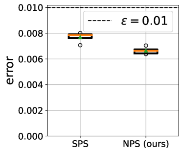
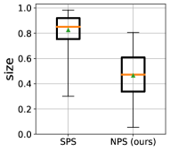
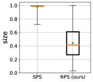
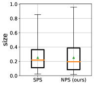
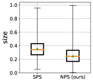
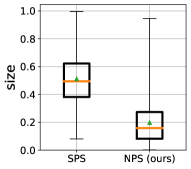
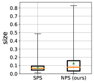
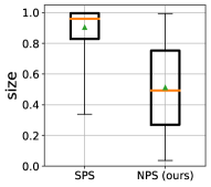
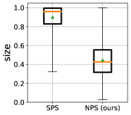
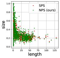
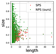
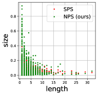
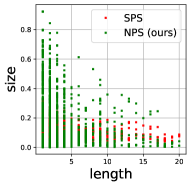
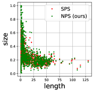
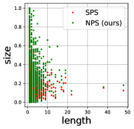
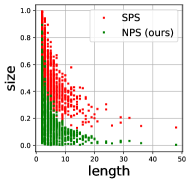
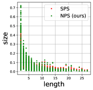
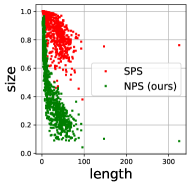
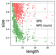
Discussion. Table 1 summarizes the performance of our method along with the baseline. All prediction set errors of both methods are below of $\varepsilon=0.01$, satisfying the PAC guarantee (i.e., the prediction set error is less than $\varepsilon$ with probability at least $1-\delta$; see Figure 5 for details). Also, NPS produces $63\%$ smaller prediction sets than the baseline on average even though we use the same number of calibration samples ($n=50,000$) for both methods but NPS holds out the half for learning $g$. These justify that NPS satisfies the PAC guarantee, while producing smaller set size than SPS.

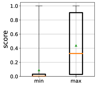
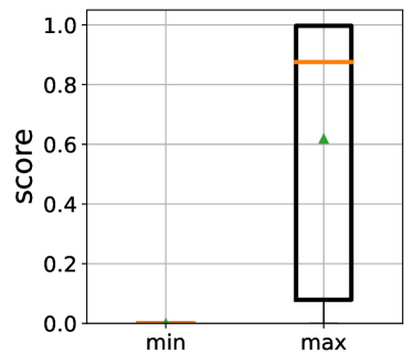
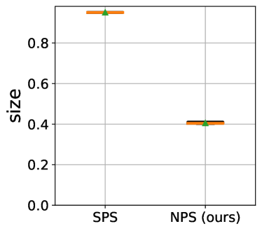
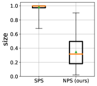
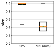
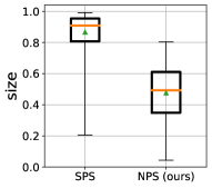
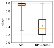
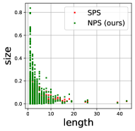
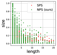
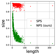
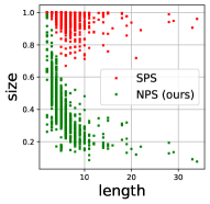
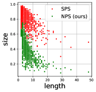
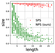
Notably, SPS tends to produce vacuous prediction sets for LLaMA-7B and Alpaca-7B models. From Figure 4(b), we observe that these models produce many small conformity scores on true labels in learning (i.e., the models are under-confident), which leads to making the prediction set error larger than $\varepsilon$. This results in very small $\hat{\tau}$ so conservative prediction sets by SPS. Contrast to this, NPS produces meaningful prediction set size, which demonstrates the benefit of a high-dimensional parameterization of prediction sets, which is viable to model a complex structure of conformity scores.

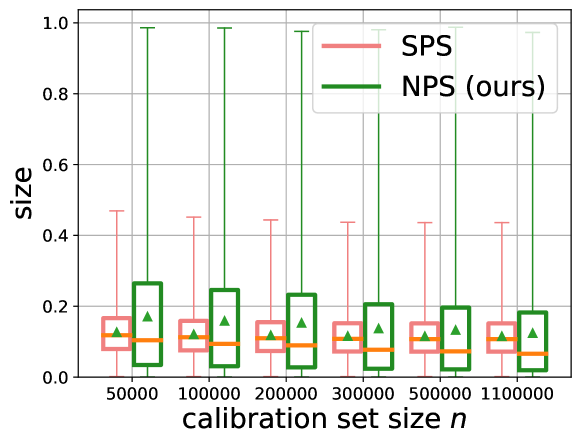
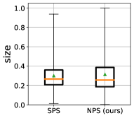
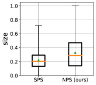
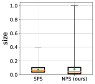
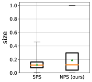
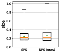
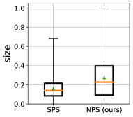
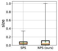
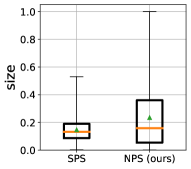
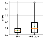
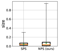
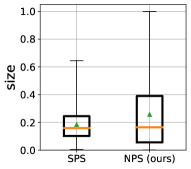
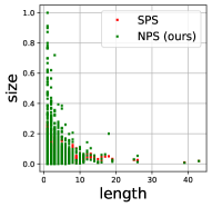
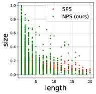
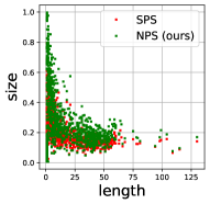
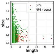
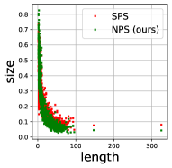
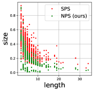
For GPT-2 models, NPS achieves competitive results in size. In particular, SPS produces relatively small set size for GPT-2 models as the conformity scores $f(\mathbf{x},\mathbf{y}_{1:l},\mathbf{y}_{l})$ of these models are distributed in a narrow range (e.g., Figure 4(a)). This implies that a simple prediction set parameter could perform well for models with non-diverse conformity scores, though we also observe that NPS with larger calibration set size clearly outperforms SPS in the median set size (see Figure 6 for details).

Figure 3 shows the qualitative results on token-wise uncertainty of Alpaca-7B over TriviaQA. SPS produces non-informative prediction sets, while NPS reasonably quantifies the token-wise uncertainty of the model (i.e., NPS sparsely shows higher uncertainty if the corresponding position has multiple alternative tokens than the generated token). Interestingly, “Bob Dylan” example shows one benefit of the PAC guarantee. As mentioned in Section 3.5, the conditional prediction set can say when a generated token is provably incorrect (i.e., Bob Dylan is not British), as visualized in red backgrounds. See Figure 10 for more results.

Question	Who was the Queen consort of King Charles the Second of England?
Desired answer	Catherine of Braganza
SPS	Catherine of Bragança.
NPS (ours)	Catherine of Bragança.

Question	Spelunking is the exploration of what, especially as a hobby?
Desired response	Caves
SPS	Spelunking is the exploration of caves or other unknown places
NPS (ours)	Spelunking is the exploration of caves or other unknown places

Question	What 1899 poem of Rudyard Kipling whose racist title alludes to Western aspirations to dominate the developing world was written after the American colonization of the Philippines?
Desired response	The White Man’s Burden
SPS	The White Man’s Burden.
NPS (ours)	The White Man’s Burden.

Question	What colour is iodine vapour?
Desired response	Violet or Purple
SPS	Iodine vapour is purple.
NPS (ours)	Iodine vapour is purple.

Question	The city of Geneva is in which European country?
Desired answer	Switzerland
SPS	Switzerland.
NPS (ours)	Switzerland.

Question	The A57 road runs from Liverpool to which English town or city?
Desired answer	Lincoln
SPS	The A57 road runs from Liverpool to Sheffield in England.
NPS (ours)	The A57 road runs from Liverpool to Sheffield in England.

Question	Name the British scientist who shared the 2013 Nobel Prize for Physics.
Desired response	Peter Higgs
SPS	The British scientist who shared the 2013 Nobel Prize for Physics is James Peebles, Michel Mayor and Didier Queloz.
NPS (ours)	The British scientist who shared the 2013 Nobel Prize for Physics is James Peebles, Michel Mayor and Didier Queloz.

Question	Who was the last British winner of the Nobel Prize for Literature?
Desired answer	Doris Lessing (2007)
SPS	The last British winner of the Nobel Prize for Literature was artist Bob Dylan in 2016.
NPS (ours)	The last British winner of the Nobel Prize for Literature was artist Bob Dylan in 2016.

Figure 3: Token-wise uncertainty results. We use the Alpaca-7B model [35] on questions from TriviaQA [15] to generate responses. Here, the uncertainty is represented in the intensity of the “red” background color, proportional to the number of alternative tokens. The proposed NPS predicts reasonable uncertainty on each token than the baseline SPS.

5 Conclusion

We propose to learn a neural prediction set for quantifying the uncertainty of GLMs, measured by the prediction set size. The proposed learning algorithm comes with the PAC guarantee, the source of trust on the quantified uncertainty. We empirically justify the efficacy of our method in various language datasets and GLMs, in terms of prediction set error and size.

Limitations. As the main limitation, the proposed method relies on the i.i.d. assumption, which can be violated via distribution shift, e.g., adversarial prompts. Extending our method under distribution shift would be an interesting future direction. Additionally, considering beyond token-wise uncertainty (e.g., semantic uncertainty) could provide more user-friendly uncertainty.

Potential negative societal impacts. The proposed method quantifies the uncertainty of GLM responses under the i.i.d. assumption. Understanding this assumption and ways to interpret uncertainty results are required to avoid misunderstanding. As a safeguard, we will provide guidelines to interpret quantified uncertainty results.

Appendix A Proof of Lemma 1

We consider the following decomposition of $\tau$ for any $g\in\mathcal{{G}}^{\prime}$:

$$\log\tau(\mathbf{x})\coloneqq g(\mathbf{x})+h.$$

Due to this, the neural prediction set for the $l$-th token is represented as follows:

$$C_{l}(\mathbf{x}) =\Big{\{}(\mathbf{y},y)\in C_{l-1}(\mathbf{x})\times\mathcal{{X}}\;\Big{|}\;f((\mathbf{x},\mathbf{y}),y)\geq\tau(\mathbf{x},\mathbf{y})\Big{\}}$$

$$=\left\{(\mathbf{y},y)\in C_{l-1}(\mathbf{x})\times\mathcal{{X}}\;\middle|\;\frac{f((\mathbf{x},\mathbf{y}),y)}{\exp{g(\mathbf{x},\mathbf{y})}}\geq\exp{h}\right\}$$

$$=\Big{\{}(\mathbf{y},y)\in C_{l-1}(\mathbf{x})\times\mathcal{{X}}\;\Big{|}\;f^{\prime}((\mathbf{x},\mathbf{y}),y)\geq\tau^{\prime}\Big{\}},$$

where $f^{\prime}((\mathbf{x},\mathbf{y}),y)\coloneqq\frac{f((\mathbf{x},\mathbf{y}),y)}{\exp{g(\mathbf{x},\mathbf{y})}}$ and $\tau^{\prime}\coloneqq\exp{h}$. Then, the error of the neural prediction set is represented as follows:

$$\mathbbm{1}\left(\mathbf{y}\notin C_{|\mathbf{y}|}(\mathbf{x})\right)=\bigvee_{l=1}^{|\mathbf{y}|}f^{\prime}((\mathbf{x},\mathbf{y}_{1:l-1}),\mathbf{y}_{l})<\tau^{\prime},$$

where the error is monotonically non-decreasing in $\tau^{\prime}$. Thus, we can use $\mathcal{{A}}_{\text{Binom}}$ in (3), which is $(\varepsilon,\delta)$-PAC for any scoring function, including $f^{\prime}$, to find $\tau^{\prime}$, proving that $\mathcal{{A}}_{h}$ is also $(\varepsilon,\delta)$-PAC.

Appendix B Implementation Details

We discuss implementation details on scalar prediction sets and neural prediction sets.

Scalar Prediction Sets for GLMs. We use the following error for the scalar prediction sets of GLMs.

$$\mathbbm{1}\left(\mathbf{y}\notin C_{|\mathbf{y}|}(\mathbf{x})\right)=\bigvee_{l=1}^{|\mathbf{y}|}f((\mathbf{x},\mathbf{y}_{1:l-1}),\mathbf{y}_{l})<\tau.$$

Compared to the error of the neural prediction sets, the only difference is the parameter of the prediction sets (i.e., $\tau$ for scalar prediction sets and $\tau(\mathbf{x})$ for neural prediction sets), but both use the recursive prediction set definition in (7).

Prediction set post-processing. The prediction set is a set of tokens, which may contain semantically similar tokens. Here, we normalize tokens by considering syntactic and semantic similarities. In particular, we convert tokens in lower cases, followed by trimming the left and right white spaces. Moreover, we use WordNet [20] to find semantically similar tokens. From these, we slightly reduce redundant tokens in a prediction set.

Appendix C Experiment Details

Dataset processing. For each category of datasets, we randomly partition the $70\%$ and $30\%$ of the entire data for a calibration set and a test set, respectively. In summary, we have $81,171$ calibration samples and $34,788$ test samples for the common sense reasoning dataset, $69,254$ calibration samples and $29,681$ test samples for the closed-book QA dataset, $81,641$ calibration samples and $34,989$ test samples for the open-book QA dataset, and $7,000,000$ calibration samples and $3,000,000$ test samples for the mathematical reasoning dataset. Note that for the closed-book QA dataset, we convert multi-choice datasets into question-answering. In calibration, we randomly sample $\mathbf{Z}$ from a calibration set and in evaluation, we randomly sample $100,000$ from a test set. For $\mathbf{Z}_{g}^{\prime}$ and $\mathbf{Z}_{g}^{\prime\prime}$ used in our method, we randomly partition the $70\%$ and $30\%$ of $\mathbf{Z}_{g}$ for $\mathbf{Z}_{g}^{\prime}$ and $\mathbf{Z}_{g}^{\prime\prime}$, respectively.

Hyperparameters for neural prediction sets. To learn $g$ for a neural prediction set, we use AdamW [18] for $100$ epochs with the initial learning rate of $0.01$, exponentially decaying by $0.95$ for each epoch. During $100$ epochs for learning, we choose the best $g$ (in terms of the same loss as (11)) by using $\mathbf{Z}_{g}^{\prime\prime}$.

Set visualization. For the visualization purpose of prediction sets (e.g., Figure 3), we rescale the set size by taking a squared root (i.e., $\sqrt{\nicefrac{{\hat{{C}}_{l}(\mathbf{x};\mathbf{y}^{\prime}_{1:l-1})}}{{|\mathcal{{X}}|}}}$) for the intensity of the red background color to amplify the small set size.

Computational environment. We use a GPU server with 128 2.3 GHz CPUs and eight NVIDIA RTX A6000 GPUs. In the worst case (i.e., obtaining NPS results for the open-book QA dataset by using LLaMA-13B), the computation takes about two days.

Appendix D Additional Experiments

(a) GPT-2 Small

(b) Alpaca-7B

Figure 4: The conformity score distribution on the closed-book QA dataset. For each model, we consider the distribution of the minimum and maximum scores among responses, i.e., $\min_{l\in\{1,\dots,|\mathbf{y}|\}}f((\mathbf{x},\mathbf{y}_{1:l-1}),\mathbf{y}_{l})$ and $\max_{l\in\{1,\dots,|\mathbf{y}|\}}f((\mathbf{x},\mathbf{y}_{1:l-1}),\mathbf{y}_{l})$ for each question and true response pair $(\mathbf{x},\mathbf{y})$. As can be seen in Figure 4(a) and Figure 4(b), the minimum and maximum scores of GPT-2 Small are closer each other than those of Alpaca-7B. This implies that Alpaca-7B is extremely certain or uncertain on the predictions of true tokens, compared to GPT-2 small. In uncertainty quantification, the proposed neural prediction set is more beneficial to capture the diverse-level of uncertainty due to a high-dimensional parameter $\tau(\mathbf{x})$ than a scalar-parameterized prediction set. Moreover, the size of the scalar-parameterized prediction set for Alpaca-7B tends to be large as there are many small scores, which makes the learned parameter $\hat{\tau}$ extremely small.

(a) Error distribution

(b) Size distribution

Figure 5: Prediction set error and size distribution over multiple-random experiments from Alpaca-7B on the mathematical reasoning dataset (with $\varepsilon=0.01$, $\delta=10^{-5}$, and $n=50,000$). We conducted 5 random experiments where each experiment randomly draws a calibration set from the entire dataset. As can be seen, the upper whisker plot, which covers the $1-\delta$ fraction of error points, is below the desired error rate $\varepsilon$, which implies that our method satisfies the PAC guarantee. The size distribution is a distribution over the mean size values of prediction sets, which is clearly smaller than the baseline method.

Figure 6: Prediction set size by varying calibration set size $n$ (with the GPT-2 Small model on the mathematical reasoning dataset). The box plot represents a distribution over the average normalized-size (i.e., $\nicefrac{{1}}{{|\mathbf{y}|}}\sum_{l=1}^{|\mathbf{y}|}\nicefrac{{\hat{{C}}(\mathbf{x};\mathbf{y}_{1:l-1})}}{{|\mathcal{{X}}|}}$); the green triangles represent mean values and the orange bars represent median values. As the calibration set size increases, we observe that NPS achieves compatible mean size and clearly better median size, compared to SPS.

	Common sense reasoning	Closed-book QA	Open-book QA	Mathematical reasoning
GPT-2 Small
GPT-2 Medium
GPT-2 Large
LLaMA-7B
LLaMA-13B
Alpaca-7B

Figure 7: Size distributions over different score functions and datasets. We visualize a size distribution where each sample for a box plot represents the average normalized-size of recursive prediction sets on a single question (i.e., $\nicefrac{{1}}{{|\mathbf{y}|}}\sum_{l=1}^{|\mathbf{y}|}\nicefrac{{\hat{{C}}(\mathbf{x};\mathbf{y}_{1:l-1})}}{{|\mathcal{{X}}|}}$).

	Common sense reasoning	Closed-book QA	Open-book QA	Mathematical reasoning
GPT-2 Small
GPT-2 Medium
GPT-2 Large
LLaMA-7B
LLaMA-13B
Alpaca-7B

Figure 8: Length and size distributions over different score functions and datasets. We illustrate the correlation between the length of a true response (i.e., $|\mathbf{y}|$) and the average normalized-size of recursive prediction sets (i.e., $\nicefrac{{1}}{{|\mathbf{y}|}}\sum_{l=1}^{|\mathbf{y}|}\nicefrac{{\hat{{C}}(\mathbf{x};\mathbf{y}_{1:l-1})}}{{|\mathcal{{X}}|}}$). As can be seen, NPS constructs smaller prediction sets than SPS as the length of the true response is longer, suggesting that a high-dimensional parameter aids to capture a complex and position-dependent structure of conformity scores for fine-grained uncertainty representation.

Figure 9: Response length distributions of each dataset. “Common” represents the common sense dataset, “Closed” represents the closed-book QA dataset, “Open” represents the open-book QA dataset, and “Math” represents the mathematical reasoning dataset. The common sense dataset tends to have longer responses, while other datasets mostly have responses shorter than 10 tokens.

Question	Who was the last British winner of the Nobel Prize for Literature?
Desired response	Doris Lessing (2007)
SPS	It was Chu Lin (Chinese 1985), and his "Trilogy of First-Person Expressions".
NPS (ours)	It was Chu Lin (Chinese 1985), and his "Trilogy of First-Person Expressions".

Question	What colour is iodine vapour?
Desired response	Violet or Purple
SPS	Iodine is yellow-orange in colour.
NPS (ours)	Iodine is yellow-orange in colour.

Question	Who was the Queen consort of King Charles the Second of England?
Desired response	Catherine of Braganza
SPS	Charles the Young Prince of Wales.
NPS (ours)	Charles the Young Prince of Wales.

Figure 10: Token-wise uncertainty results. We use the GPT-2 Large model [31] on questions from TriviaQA [15] to generate responses. Here, the uncertainty is represented in the intensity of the “red” background color, proportional to the number of alternative tokens. The quantified uncertainty on each token by the proposed NPS and the baseline is similar, even though the prediction set size of the baseline is quantitatively better in Table 1, i.e., $0.1399$ for SPS and $0.2347$ for NPS. This shows that SPS is quantitatively better but quantitatively comparable to NPS.

References

- [1] Anastasios Nikolas Angelopoulos, Stephen Bates, Michael Jordan, and Jitendra Malik. Uncertainty sets for image classifiers using conformal prediction. In International Conference on Learning Representations, 2021.
- [2] Sanjeev Arora, Simon Du, Wei Hu, Zhiyuan Li, and Ruosong Wang. Fine-grained analysis of optimization and generalization for overparameterized two-layer neural networks. In International Conference on Machine Learning, pages 322–332. PMLR, 2019.
- [3] Peter L. Bartlett, Nick Harvey, Chris Liaw, and Abbas Mehrabian. Nearly-tight vc-dimension and pseudodimension bounds for piecewise linear neural networks, 2017.
- [4] Stephen Bates, Anastasios Angelopoulos, Lihua Lei, Jitendra Malik, and Michael I Jordan. Distribution-free, risk-controlling prediction sets. arXiv preprint arXiv:2101.02703, 2021.
- [5] Yonatan Bisk, Rowan Zellers, Ronan Le Bras, Jianfeng Gao, and Yejin Choi. Piqa: Reasoning about physical commonsense in natural language, 2019.
- [6] Tom B. Brown, Benjamin Mann, Nick Ryder, Melanie Subbiah, Jared Kaplan, Prafulla Dhariwal, Arvind Neelakantan, Pranav Shyam, Girish Sastry, Amanda Askell, Sandhini Agarwal, Ariel Herbert-Voss, Gretchen Krueger, Tom Henighan, Rewon Child, Aditya Ramesh, Daniel M. Ziegler, Jeffrey Wu, Clemens Winter, Christopher Hesse, Mark Chen, Eric Sigler, Mateusz Litwin, Scott Gray, Benjamin Chess, Jack Clark, Christopher Berner, Sam McCandlish, Alec Radford, Ilya Sutskever, and Dario Amodei. Language models are few-shot learners, 2020.
- [7] Yuan Cao and Quanquan Gu. Generalization bounds of stochastic gradient descent for wide and deep neural networks. Advances in neural information processing systems, 32, 2019.
- [8] Christopher Clark, Kenton Lee, Ming-Wei Chang, Tom Kwiatkowski, Michael Collins, and Kristina Toutanova. Boolq: Exploring the surprising difficulty of natural yes/no questions, 2019.
- [9] Simon S. Du, Xiyu Zhai, Barnabas Poczos, and Aarti Singh. Gradient descent provably optimizes over-parameterized neural networks. In International Conference on Learning Representations, 2019.
- [10] Adam Fisch, Tal Schuster, Tommi Jaakkola, and Regina Barzilay. Few-shot conformal prediction with auxiliary tasks, 2021.
- [11] Philip Gage. A new algorithm for data compression. C Users Journal, 12(2):23–38, 1994.
- [12] Isaac Gibbs and Emmanuel Candès. Adaptive conformal inference under distribution shift, 2021.
- [13] Chuan Guo, Geoff Pleiss, Yu Sun, and Kilian Q Weinberger. On calibration of modern neural networks. arXiv preprint arXiv:1706.04599, 2017.
- [14] Zhengbao Jiang, Jun Araki, Haibo Ding, and Graham Neubig. How Can We Know When Language Models Know? On the Calibration of Language Models for Question Answering. Transactions of the Association for Computational Linguistics, 9:962–977, 09 2021.
- [15] Mandar Joshi, Eunsol Choi, Daniel Weld, and Luke Zettlemoyer. TriviaQA: A large scale distantly supervised challenge dataset for reading comprehension. In Proceedings of the 55th Annual Meeting of the Association for Computational Linguistics (Volume 1: Long Papers), pages 1601–1611, Vancouver, Canada, July 2017. Association for Computational Linguistics.
- [16] Adam Khakhar, Stephen Mell, and Osbert Bastani. Pac prediction sets for large language models of code, 2023.
- [17] Margaret Li, Stephen Roller, Ilia Kulikov, Sean Welleck, Y-Lan Boureau, Kyunghyun Cho, and Jason Weston. Don’t say that! making inconsistent dialogue unlikely with unlikelihood training. In Proceedings of the 58th Annual Meeting of the Association for Computational Linguistics, pages 4715–4728, Online, July 2020. Association for Computational Linguistics.
- [18] Ilya Loshchilov and Frank Hutter. Decoupled weight decay regularization, 2019.
- [19] Sabrina J. Mielke, Arthur Szlam, Emily Dinan, and Y-Lan Boureau. Reducing Conversational Agents’ Overconfidence Through Linguistic Calibration. Transactions of the Association for Computational Linguistics, 10:857–872, 08 2022.
- [20] George A. Miller. WordNet: A lexical database for English. In Human Language Technology: Proceedings of a Workshop held at Plainsboro, New Jersey, March 8-11, 1994, 1994.
- [21] Allan H Murphy. Scalar and vector partitions of the probability score: Part i. two-state situation. Journal of Applied Meteorology, 11(2):273–282, 1972.
- [22] OpenAI Team. ChatGPT. https://chat.openai.com/, 2021.
- [23] Long Ouyang, Jeff Wu, Xu Jiang, Diogo Almeida, Carroll L. Wainwright, Pamela Mishkin, Chong Zhang, Sandhini Agarwal, Katarina Slama, Alex Ray, John Schulman, Jacob Hilton, Fraser Kelton, Luke Miller, Maddie Simens, Amanda Askell, Peter Welinder, Paul Christiano, Jan Leike, and Ryan Lowe. Training language models to follow instructions with human feedback, 2022.
- [24] Harris Papadopoulos, Kostas Proedrou, Volodya Vovk, and Alex Gammerman. Inductive confidence machines for regression. In European Conference on Machine Learning, pages 345–356. Springer, 2002.
- [25] Sangdon Park, Osbert Bastani, and Taesoo Kim. Acon2: Adaptive conformal consensus for provable blockchain oracles, 2023.
- [26] Sangdon Park, Osbert Bastani, Nikolai Matni, and Insup Lee. Pac confidence sets for deep neural networks via calibrated prediction. In International Conference on Learning Representations, 2020.
- [27] Sangdon Park, Edgar Dobriban, Insup Lee, and Osbert Bastani. PAC prediction sets for meta-learning. In Alice H. Oh, Alekh Agarwal, Danielle Belgrave, and Kyunghyun Cho, editors, Advances in Neural Information Processing Systems, 2022.
- [28] Sangdon Park, Edgar Dobriban, Insup Lee, and Osbert Bastani. PAC prediction sets under covariate shift. In International Conference on Learning Representations, 2022.
- [29] Sangdon Park, Shuo Li, Insup Lee, and Osbert Bastani. PAC confidence predictions for deep neural network classifiers. In International Conference on Learning Representations, 2021.
- [30] John Platt. Probabilistic outputs for support vector machines and comparisons to regularized likelihood methods. Advances in large margin classifiers, 1999.
- [31] Alec Radford, Jeffrey Wu, Rewon Child, David Luan, Dario Amodei, Ilya Sutskever, et al. Language models are unsupervised multitask learners. OpenAI blog, 1(8):9, 2019.
- [32] Siva Reddy, Danqi Chen, and Christopher D. Manning. Coqa: A conversational question answering challenge, 2019.
- [33] Maarten Sap, Hannah Rashkin, Derek Chen, Ronan LeBras, and Yejin Choi. Socialiqa: Commonsense reasoning about social interactions. arXiv preprint arXiv:1904.09728, 2019.
- [34] David Saxton, Edward Grefenstette, Felix Hill, and Pushmeet Kohli. Analysing mathematical reasoning abilities of neural models. In International Conference on Learning Representations, 2019.
- [35] Rohan Taori, Ishaan Gulrajani, Tianyi Zhang, Yann Dubois, Xuechen Li, Carlos Guestrin, Percy Liang, and Tatsunori B. Hashimoto. Stanford alpaca: An instruction-following llama model. https://github.com/tatsu-lab/stanford_alpaca, 2023.
- [36] Hugo Touvron, Thibaut Lavril, Gautier Izacard, Xavier Martinet, Marie-Anne Lachaux, Timothée Lacroix, Baptiste Rozière, Naman Goyal, Eric Hambro, Faisal Azhar, Aurelien Rodriguez, Armand Joulin, Edouard Grave, and Guillaume Lample. Llama: Open and efficient foundation language models, 2023.
- [37] Leslie G Valiant. A theory of the learnable. Communications of the ACM, 27(11):1134–1142, 1984.
- [38] Ashish Vaswani, Noam Shazeer, Niki Parmar, Jakob Uszkoreit, Llion Jones, Aidan N Gomez, Lukasz Kaiser, and Illia Polosukhin. Attention is all you need. Advances in neural information processing systems, 30, 2017.
- [39] Vladimir Vovk. Conditional validity of inductive conformal predictors. Machine learning, 92(2-3):349–376, 2013.
- [40] Vladimir Vovk, Alex Gammerman, and Glenn Shafer. Algorithmic learning in a random world. Springer Science & Business Media, 2005.
- [41] Samuel S Wilks. Determination of sample sizes for setting tolerance limits. The Annals of Mathematical Statistics, 12(1):91–96, 1941.
- [42] Bianca Zadrozny and Charles Elkan. Obtaining calibrated probability estimates from decision trees and naive bayesian classifiers. In In Proceedings of the Eighteenth International Conference on Machine Learning. Citeseer, 2001.
- [43] Bianca Zadrozny and Charles Elkan. Transforming classifier scores into accurate multiclass probability estimates. In Proceedings of the eighth ACM SIGKDD international conference on Knowledge discovery and data mining, pages 694–699. ACM, 2002.
- [44] Rowan Zellers, Ari Holtzman, Yonatan Bisk, Ali Farhadi, and Yejin Choi. Hellaswag: Can a machine really finish your sentence? arXiv preprint arXiv:1905.07830, 2019.