Laboratory and astronomical discovery of the cyanovinyl radical H₂CCCN

We report the first laboratory and interstellar detection of the $\alpha$-cyano vinyl radical (H₂CCCN). This species was produced in the laboratory by an electric discharge of a gas mixture of vinyl cyanide, CH₂CHCN, and Ne, and its rotational spectrum was characterized using a Balle-Flygare narrowband-type Fourier-transform microwave spectrometer operating in the frequency region of 8-40 GHz. The observed spectrum shows a complex structure due to tunneling splittings between two torsional sublevels of the ground vibronic state, $0^{+}$ and $0^{-}$, derived from a large-amplitude inversion motion. In addition, the presence of two equivalent hydrogen nuclei makes necessary to discern between ortho- and para-H₂CCCN. A least squares analysis reproduces the observed transition frequencies with a standard deviation of ca. 3 kHz. Using the laboratory predictions, this radical is detected in the cold dark cloud TMC-1 using the Yebes 40m telescope and the QUIJOTE¹ line survey. The 4_0,4-3_0,3 and 5_0,5-4_0,4 rotational transitions, composed of several hyperfine components, were observed in the 31.0-50.4 GHz range. Adopting a rotational temperature of 6 K we derive a column density of (1.4$\pm$0.2)$\times$10¹¹ cm^-2 and (1.1$\pm$0.2)$\times$10¹¹ cm^-2 for ortho-H₂CCCN and para-H₂CCCN, respectively. The reactions C + CH₃CN, and perhaps also N + CH₂CCH, emerge as the most likely routes to H₂CCCN in TMC-1.

1 Introduction

Vinyl cyanide, CH₂CHCN, is a well known interstellar molecule that was detected for the first time in the interstellar medium (ISM) in 1973 toward the Sagittarius B2 (Sgr B2) molecular cloud (Gardner & Winnewisser 1975). Since then, vinyl cyanide has been detected toward different sources, such as Orion (Schilke et al. 1997), the dark cloud TMC-1 (Matthews & Sears 1983), the circumstellar envelope of the late-type star IRC+10216 (Agúndez et al. 2008), and the Titan atmosphere (Capone et al. 1981). Vinyl cyanide is one of the molecules, whose high abundance and significant dipole moment allow radioastronomical detection even of its rare isotopologue species and vibrationally excited states (López et al. 2014). Thus, the cyanovinyl radical (CVR) is a promising candidate for its interstellar detection given its similarity to the aforementioned vinyl cyanide. This hypothesis is strengthened by the recent detection of the H₂C₄N radical (Cabezas et al. 2021) with the QUIJOTE line survey (Cernicharo et al. 2021, 2023).

The CVR has two structural isomers depending on whether the $\alpha$- or $\beta$-hydrogen, -CH or CH₂, respectively, of vinyl cyanide is removed. The molecular formula H₂CCCN corresponds to the $\alpha$-CVR while HCCHCN formula is that for $\beta$-CVR, which further allows the cis and trans isomers. Quantum chemical calculation indicate that the $\alpha$-CVR is more stable in energy than the $\beta$-CVR by 30–45 kJ mol^-1 (Balucani et al. 2000; Huang et al. 2000; Johansen et al. 2019). The rotational spectra of both isomers of the $\beta$-CVR have been investigated by Johansen et al. (2019) and Nakajima et al. (2022). In their study, Johansen et al. (2019) observed several rotational transitions for both cis and trans isomers of $\beta$-CVR in the 5-75 GHz frequency range but no conclusive assignments of the fine and hyperfine components was reported. On the other hand, Nakajima et al. (2022) reported precise molecular constants for the cis isomer of $\beta$-CVR thanks to the deep analysis of all the fine and hyperfine components observed in the 10-55 GHz region. However, no spectroscopic data for the $\alpha$-CVR have been reported before in the literature, except our preliminary results (Tang et al. 2000).

In this Letter we report the first rotational investigation study of the $\alpha$-CVR, hereafter H₂CCCN, and the discovery of this radical in space towards TMC-1. The laboratory characterization has been done using Fourier transform microwave (FTMW) spectroscopy in combination to electric discharges techniques. The identification of this radical in space has been done using the on-going QUIJOTE line survey (Cernicharo et al. 2021, 2023).

2 Laboratory FTMW spectroscopy of H₂CCCN

The rotational spectrum of H₂CCCN was observed using a Balle-Flygare narrowband type FTMW spectrometer operating in the frequency region of 4-40 GHz (Endo et al. 1994; Cabezas et al. 2016). The short-lived species H₂CCCN was produced in a supersonic expansion by a pulsed electric discharge of a gas mixture of CH₂CHCN (0.2%) diluted in Ne. This gas mixture was flowed through a pulsed-solenoid valve that is accommodated in the backside of one of the cavity mirrors and aligned parallel to the optical axis of the resonator. A pulse voltage of 900 V with a duration of 450 $\mu$s was applied between stainless steel electrodes attached to the exit of the pulsed discharge nozzle (PDN), resulting in an electric discharge synchronized with the gas expansion. The resulting products generated in the discharge were supersonically expanded, rapidly cooled to a rotational temperature of $\sim$2.5 K between the two mirrors of the Fabry-Pérot resonator, and then probed by FTMW spectroscopy. For measurements of the paramagnetic lines, the Earth’s magnetic field was cancelled by using three sets of Helmholtz coils placed perpendicularly to one another. Since the PDN is arranged parallel to the cavity of the spectrometer, it is possible to suppress the Doppler broadening of the spectral lines, allowing to resolve small hyperfine splittings. The spectral resolution is 5 kHz and the frequency measurements have an estimated accuracy better than 3 kHz.

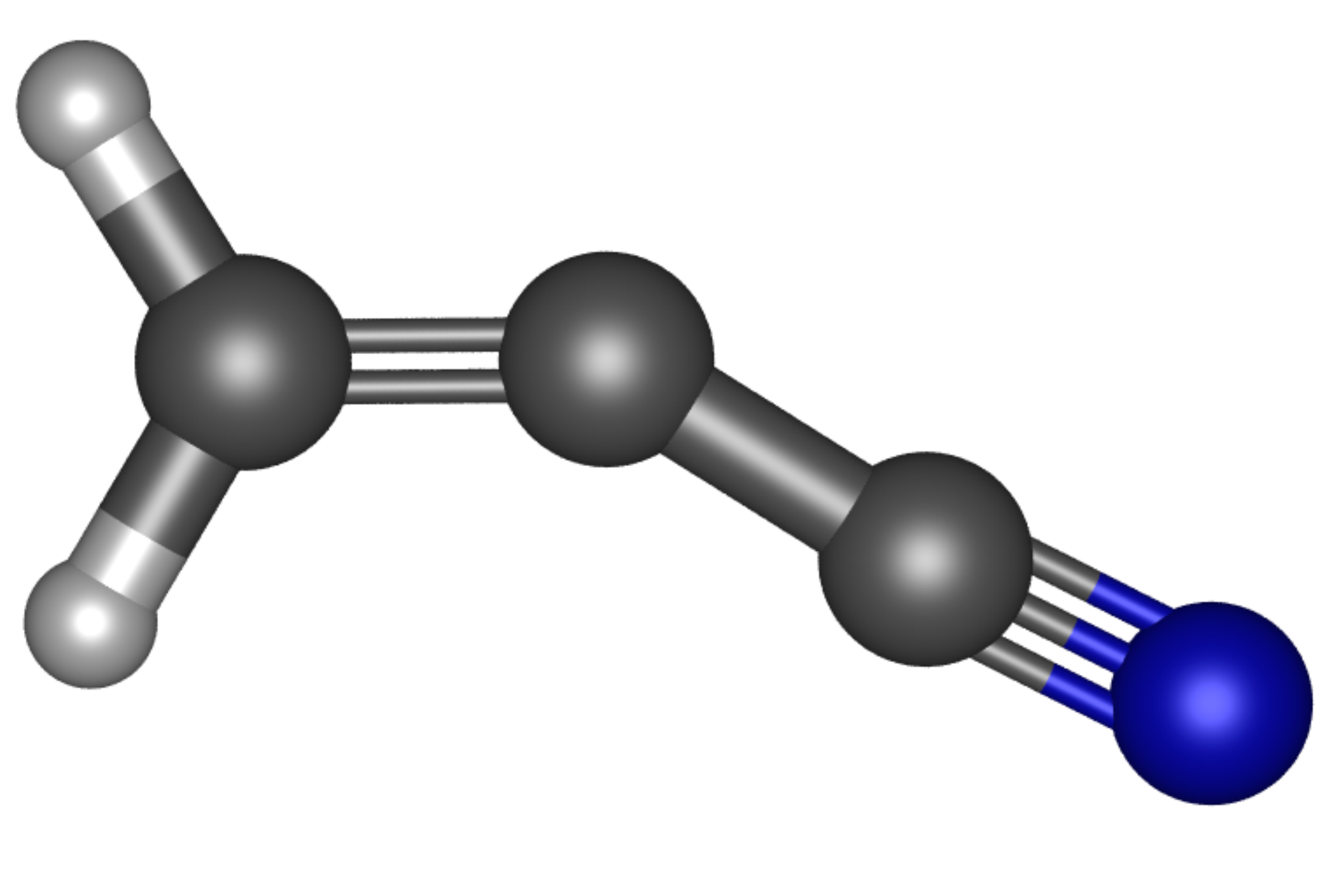
Figure 1: Molecular structure of the H₂CCCN radical.

3 Astronomical observations

New receivers, built within the Nanocosmos project and installed at the Yebes 40 m radiotelescope, were used for the observations of TMC-1 ($\alpha_{J2000}=4^{\rm h}41^{\rm m}41.9^{\rm s}$ and $\delta_{J2000}=+25^{\circ}41^{\prime}27.0^{\prime\prime}$). A detailed description of the telescope, receivers, and backends is given by Tercero et al. (2021). Briefly, the receiver consists of two cold high electron mobility transistor amplifiers covering the 31.0-50.3 GHz band with horizontal and vertical polarizations. The backends are $2\times 8\times 2.5$ GHz fast Fourier transform spectrometers with a spectral resolution of 38.15 kHz providing the whole coverage of the Q-band in both polarisations. The observations, carried out during different observing runs, are performed using the frequency-switching mode with a frequency throw of 10 MHz in the very first observing runs, during November 2019 and February 2020, 8 MHz during the observations of January-November 2021, and alternating these frequency throws in the last observing runs between October 2021 and February 2023. The total on-source telescope time is 850 hours in each polarization (385 and 465 hours for the 8 MHz and 10 MHz frequency throws, respectively). The sensitivity of the QUIJOTE line survey varies between 0.09 and 0.25 mK in the 31-50.3 GHz domain. The intensity scale used in this work, antenna temperature ($T_{A}^{*}$), was calibrated using two absorbers at different temperatures and the atmospheric transmission model ATM (Cernicharo 1985; Pardo et al. 2001). Calibration uncertainties have been adopted to be 10 %. The beam efficiency of the Yebes 40 m telescope in the Q-band is given as a function of frequency by $B_{\rm eff}$= 0.797 exp[$-$($\nu$(GHz)/71.1)²]. The forward telescope efficiency is 0.95. The telescope beam size varies from 56.7^′′ at 31 GHz to 35.6^′′ at 49.5 GHz. All data were analyzed using the GILDAS package.

4 Results

4.1 Quantum chemical calculations of H₂CCCN

Several theoretical calculations have been done on the H₂CCCN radical. Fenistein et al. (1969) and Hinchliffe (1977) calculated only the $C_{2v}$-symmetry structure in that two protons are equivalent relative to the linear carbon-chain backbone. Later, Mayer et al. (1998) and Parkinson et al. (1999) predicted a stable $C_{s}$-symmetry structure, both using density functional theory calculations, with the bending angle $\angle$CCC=164.9^∘ and in the standard coupled cluster approach level with $\angle$CCC=149.1^∘ (Parkinson et al. 1999). The energy barrier from the $C_{s}$ minimum to the $C_{2v}$ saddle point of H₂CCCN was calculated to be 1190 cm^-1 (Parkinson et al. 1999).

We optimized the geometry of the H₂CCCN radical at the spin-restricted coupled cluster method with single, double, and perturbative triple excitations (RCCSD(T)) and an explicitly correlated approximation (F12A) (Adler et al. 2007; Knizia et al. 2009) with all electrons (valence and core) correlated and the Dunning’s correlation consistent basis sets with polarized core-valence triple-$\zeta$ for explicitly correlated calculations (cc-pCVTZ-F12; Hill et al. 2010a, b). At the optimized geometry, electric dipole moment components were calculated at the same level of theory as that for the geometrical optimization. We derive a value for $\mu_{a}$ of 3.6 D. The H₂CCCN radical in the ${}^{2}A^{\prime}$ ground electronic state adopts a bent geometry with a $\angle$CCC angle of 147^∘, as it can be seen in Fig. 1. Using RCCSD(T)-F12/cc-pCVTZ-F12 level of theory we obtained the inversion barrier of $V_{i}$ = 356 cm^-1 at the C_2v saddle point. These calculations were performed using the Molpro 2020 ab initio program package (Werner et al. 2020).

The fine and hyperfine coupling constants were estimated using the B3LYP hybrid density functional (Becke 1993) with the augmented diffuse basis set (aug-cc-pVTZ; Woon & Dunning 1995). Harmonic and anharmonic vibrational frequencies were computed using second-order Møller-Plesset perturbation (MP2; Møller & Plesset 1934) with the cc-pVTZ basis set (Woon & Dunning 1995) level of theory to estimate the centrifugal distortion constants and the vibration–rotation interaction contribution to the rotational constants. These calculations were performed using the Gaussian16 program package (Frisch et al. 2016). The calculated molecular parameters are summarized in Table 1.

4.2 Rotational spectrum of H₂CCCN

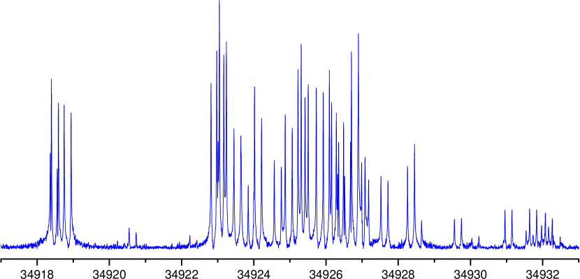
Figure 2: FTMW spectrum for the H₂CCCN radical showing the 4_0,4-3_0,3 rotational transition at 34.9 GHz. Much weaker additional hyperfine components, which are not shown in this figure, were also observed. The abscissa corresponds to the frequency of the lines in MHz. The spectra were achieved by 200 shots of accumulation and a step scan of 1 MHz with a repetition rate of 10 Hz. The coaxial arrangement of the adiabatic expansion and the resonator axis produces an instrumental Doppler doubling. The resonance frequencies are calculated as the average of the two Doppler components.

Due to the bent geometry for H₂CCCN radical in the ${}^{2}A^{\prime}$ ground state, there are two equivalent configurations which correspond to different minima of the double minimum potential of the inversion motion. This pair of tunneling inversion states $\nu_{inv}$=$0^{\pm}$, will originate a doublet pattern in the rotational spectrum for H₂CCCN. Required by the Pauli’s exclusion principle, ortho and para species due to two hydrogen nuclei in H₂CCCN correspond to the inversion states $0^{+}$ and $0^{-}$, respectively, in the even $K_{a}$ rotational levels. For odd $K_{a}$ rotational levels ortho/para changes and $0^{+}$ is para, while $0^{-}$ is ortho. The $0^{+}$ level is considered to be always the lower splitting sublevel.

A total of four groups of paramagnetic lines around 8.7 GHz, 17.4 GHz, 26.2 GHz, and 34.9 GHz were observed in our experiment. An example is shown in Fig. 2. The H₂CCCN radical was readily confirmed as the spectral carrier based on the following arguments. (i) The observed transition frequencies agree well with the calculated frequencies, (ii) each transition has a hyperfine spectral structure similar to that expected for an open-shell species with three coupling nuclei, and (iii) the lines exhibit the paramagnetic behavior.

Assignment of the fine and hyperfine structure was first achieved for the spectrum of para-H₂CCCN ($K_{a}$ = 0 transitions for $0^{-}$ sublevel), in which the higher-$N$ transitions presented relatively simple structures. By a least-squares fitting, the spin-rotation interaction constants and the hyperfine interaction constants for the nitrogen nucleus were determined, where hyperfine interaction constants for the two hydrogen nuclei cannot be determined due to I(2H) = 0 in para-H₂CCCN, since this species has parity +1 for the $a$-axis rotation. Then the remaining H₂CCCN transition lines were assigned to the ortho-H₂CCCN ($K_{a}$ = 0 transitions for $0^{+}$ sublevel) spectrum. Slightly different effective molecular constants from the ones of para-H₂CCCN including the hyperfine interaction constants for the two hydrogen nuclei were obtained for ortho-H₂CCCN with I(2H) = 1, parity -1 for the $a$-axis rotation. A total of 36 and 137 hyperfine components from $K_{a}$=0 rotational transitions were measured for para-H₂CCCN and ortho-H₂CCCN species, respectively ( see Tables LABEL:lab_freq_1 and LABEL:lab_freq_2).

All the lines for each species were independently analyzed using a standard Hamiltonian for an asymmetric top molecule with a doublet electronic state (${}^{2}A^{{}^{\prime}}$) and three non-zero-spin nuclei. The coupling scheme for angular momenta of rotation N, electron spin S, and nuclear spins I of two equivalent protons and one nitrogen nucleus is J = N + S, F₁ = J + I_H, and F = F₁ + I_N. The molecular constants derived from the analysis are shown in Table 1.

Although we have succeeded in assigning and analyzing the H₂CCCN spectra of the $K_{a}$ = 0 transitions by considering a tunneling inversion effect and by applying an effective Hamiltonian to the ortho/para species, information of the tunneling inversion motion, such as inversion barrier $V_{i}$, inversion-vibration frequency $\nu_{i}$, and inversion-vibration splitting $\delta$$\nu_{i}$^±, could not be obtained directly from our spectral analysis. The abnormally large inversion-vibration dependence of the $(B+C)$/2 constant indicated that there is a strong rotation-dependent perturbation in this radical.

Table 1: Spectroscopic parameters of H₂CCCN (all in MHz).

Parameter	ortho-H2CCCN	para-H2CCCN	Theoretical a
$A$	[158105.0] b	[158105.0]	158105.0
$(B+C)/2$	4365.86049(12) c	4365.30705(21)	4382.2
$B-C$	[120.0]	[120.0]	120.0
$\Delta_{N}$	0.0009124(48)	0.0015943(86)	0.00182
$\Delta_{NK}$	[$-$0.338]	[$-$0.338]	$-$0.338
$\Delta_{K}$	[39.10]	[39.10]	39.10
$\delta_{N}$	[0.000276]	[0.000276]	0.000276
$\delta_{K}$	[0.430]	[0.430]	0.430
$\varepsilon_{aa}$	[278.0]	[278.0]	278.0
$\varepsilon_{bb}$	[0.489]	[0.489]	0.489
$\varepsilon_{cc}$	$-$12.42269(86)	$-$12.83977(91)	$-$10.3
$a_{F}$(N)	9.58207(87)	9.50926(99)	2.71
$T_{aa}$(N)	$-$14.4086(17)	$-$14.3071(15)	$-$15.8
$T_{bb}$(N)	[26.3]	[26.3]	26.3
$\chi_{aa}$(N)	$-$4.0506(19)	$-$4.0606(32)	$-$4.43
$\chi_{aa}$(N)	[2.18]	[2.18]	2.18
$a_{F}$(H)	131.627(89)	$-$	117.7
$T_{aa}$(H)	6.4816(16)	$-$	6.82
$T_{bb}$(H)	[$-$1.97]	$-$	$-$1.97
$N_{lines}$	137	36	$-$
$rms$ /kHz	2.9	2.6	$-$

4.3 Detection of H₂CCCN in TMC-1

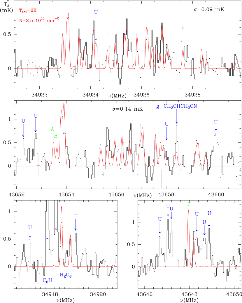
Figure 3: Observed rotational transitions of H₂CCCN in TMC-1 in the 31.0-50.4 GHz range. The abscissa corresponds to the rest frequency, assuming a local standard of rest velocity of 5.83 km s^-1. The ordinate is antenna temperature in millikelvins. Curves shown in red are the computed synthetic spectra for T_rot=6 K, N(ortho-H₂CCCN)=1.4$\times$10¹¹ cm^-2 and N(para-H₂CCCN)=1.1$\times$10¹¹ cm^-2.

Using the molecular constants derived for ortho- and para-H₂CCCN, we predicted the rotational spectra of each species. We considered the ortho and para species separately as there are no radiative or collisional transitions between them. The predictions for ortho-H₂CCCN include the rotational transitions with $K_{a}$ even for the 0⁺ sublevel and those with $K_{a}$ odd for 0^- sublevel, while para-H₂CCCN predictions contain the rotational transitions with $K_{a}$ even for the 0^- sublevel and those with $K_{a}$ odd for 0⁺ sublevel. Predictions for $K_{a}$=0 transitions have uncertainties smaller than 30 kHz up to $N$=10. They were implemented in the MADEX code (Cernicharo 2012) to compute column densities. We adopted a dipole moment of 3.60 D as derived from our calculations.

Two rotational transitions for H₂CCCN with $K_{a}$ = 0 are covered by our QUIJOTE survey, at 34.9 and 43.6 GHz. We observed two groups of lines at the predicted frequencies for the 4_0,4-3_0,3 and 5_0,5-4_0,4 transitions. Figure 3 shows the lines corresponding to these rotational transitions. More than 30 hyperfine components are observed in TMC-1 with a sensitivity of 0.09 mK for $N$=4 and of 0.14 mK for $N$=5. Our frequency switching observing procedure affects to some of these lines. The forest of lines for each transition covers more than 10 MHz (see Fig. 3) and, hence, the hyperfine components separated by 8 or 10 MHz, i.e., the frequency throws of the observations, will affect each other. In addition, at this level of sensitivity, transitions from other species and from unidentified lines could also affect the observed intensities. Some of the blends arising between the lines and their negative features at $\pm$8 MHz and $\pm$10 MHz produced in the folding of the frequency switching, have been identified and blanked in the data. As an example, the lines of C₆H and H₂C₆ appearing around 34918 MHz in the bottom left panel of the figure, will have negative counterparts at 34926 and 34928 MHz, which are within the frequency range of the $4_{0,4}-3_{0,3}$ transition. The corresponding channels have been cleaned in the top panel of Fig. 3. Three hyperfine components labelled as A, B and C in Fig. 3 are affected by other lines of H₂CCCN and by unidentified lines. For other blending situations the removal of the negative feature is much more delicate and has not been performed in the final data presented in Fig. 3. It is worth nothing to note that each of the negative features produced by a line will have half of its intensity, which for the strongest features of Fig. 3, means intensities of 0.3-0.4 mK. Nevertheless, the number of detected lines is large enough to support the identification of H₂CCCN in TMC-1 and to ensure a reliable determination of the column density.

The observed lines of H₂CCCN correspond to transitions with upper energy levels of 4.2 and 6.3 K for $N$=4 and 5, respectively. Hence, the rotational temperature (T_rot) can not be derived in a reasonable way from the observations, except if it is rather low. We have explored values for T_rot between 5 and 10 K and found that the derived column density for the two inversion states is not very sensitive to the adopted value for T_rot (see, e.g., Cernicharo et al. 2021). In order to estimate the expected rotational temperature of the 4_0,4-3_0,3 and 5_0,5-4_0,4 transitions of H₂CCCN, we have analyzed the excitation conditions of a similar molecule, H₂CCC. For this species, the collisional rates are available (Khalifa et al. 2019), and the dipole moment is also similar to that of our molecule. For a volume density of 2-3$\times$10⁴ cm^-3, typical of TMC-1, and assuming optically thin emission, we obtain rotational temperatures between 5.6-7 K for the $J_{u}$=4 and 5 transitions of H₂CCC. Adopting a value of 6 K for the two observed transitions of H₂CCCN, we derive a column density of (1.4$\pm$0.2)$\times$10¹¹ cm^-2 and of (1.1$\pm$0.2)$\times$10¹¹ cm^-2 for ortho-H₂CCCN and para-H₂CCCN, respectively. These column densities indicate that, within the uncertainties, both inversion states are equally populated. Adopting a rotational temperature of 7 K introduces an increase of the column density of $\sim$10%.

Two additional transitions for each value of $N$ corresponding to $K_{a}$=1 could be also within the QUIJOTE frequency coverage. However, the frequency predictions for these lines are unreliable as the $A$ rotational constant value has not been determined from the laboratory data. Moreover, using the value of the constant $A$ estimated from our calculations, the upper rotational levels of these $K_{a}$=1 transitions will be around 14 K. Hence, for rotational temperatures below 10 K the intensity of these lines is expected to be much lower than those of the transitions with $K_{a}$=0, and below the sensitivity of QUIJOTE.

5 Chemistry of H₂CCCN

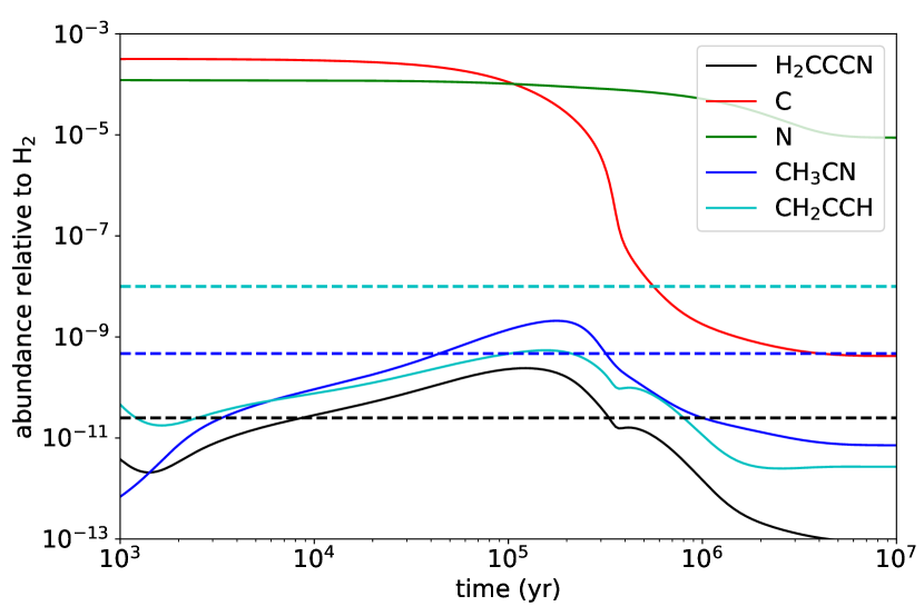
Figure 4: Abundances calculated with the chemical model for H₂CCCN and for its potential precursors. The horizontal dashed lines correspond to the values observed in TMC-1: H₂CCCN (this work), CH₃CN (Cabezas et al. 2021), and CH₂CCH (Agúndez et al. 2022).

There are several chemical reactions that can form H₂CCCN in TMC-1, although there is little experimental or theoretical information on most of them. In fact, the chemical databases UMIST (McElroy et al. 2013) and KIDA (Wakelam et al. 2015) do not contain any reaction of formation of H₂CCCN. Among the potential routes to H₂CCCN we can consider the following neutral-neutral reactions which happen with H atom elimination:

$$\rm C+CH_{3}CN\rightarrow H_{2}CCCN+H,$$ (1)

$$\rm CH+CH_{2}CN\rightarrow H_{2}CCCN+H,$$ (2)

$$\rm C_{2}H+H_{2}CN\rightarrow H_{2}CCCN+H,$$ (3)

$$\rm C_{2}H_{3}+CN\rightarrow H_{2}CCCN+H.$$ (4)

$$\rm N+CH_{2}CCH\rightarrow H_{2}CCCN+H.$$ (5)

$$\rm NH+H_{2}C_{3}\rightarrow H_{2}CCCN+H.$$ (6)

$$\rm NH_{2}+C_{3}H\rightarrow H_{2}CCCN+H.$$ (7)

To evaluate whether these reactions can produce H₂CCCN with an abundance similar to that observed we plugged them into a chemical model. We used as starting point the chemical model built by Cabezas et al. (2021) to study the chemistry of CH₂CCCN, which uses the chemical network RATE12 from the UMIST database (McElroy et al. 2013), with updates from Loison et al. (2014) and Marcelino et al. (2021). The physical parameters assumed are the typical ones of cold dark clouds, i.e., a density of H nuclei of 2 $\times$ 10⁴ cm^-3, a gas kinetic temperature of 10 K, a cosmic-ray ionization rate of H₂ of 1.3 $\times$ 10^-17 s^-1, a visual extinction of 30 mag, and the set of low-metal elemental abundances (see, e.g., Agúndez & Wakelam 2013). We added H₂CCCN as new species and included the above seven neutral-neutral reactions with a rate coefficient of 10^-10 cm³ s^-1, which is typical of neutral-neutral reactions that are fast at low temperature. We considered that H₂CCCN is destroyed by reacting with neutral atoms, such as H, O, N, and C, with a rate coefficient of 10^-10 cm³ s^-1, and with abundant positive cations, such as H⁺ and C⁺, with a rate coefficient of 10^-9 cm³ s^-1 at 300 K and a dependence with temperature of the type $T^{-0.5}$.

The results are shown in Fig. 4. The first conclusion is that H₂CCCN is indeed produced with a peak abundance of the order of the observed value at a time of a few 10⁵ yr. The second conclusion is that the main reactions of formation of H₂CCCN are by far reactions (1) and (5), because they involve as reactants atomic carbon and atomic nitrogen, respectively, which are very abundant (see Fig. 4). Interestingly, reaction (1) has been recently studied by Hickson et al. (2021). These authors measured the rate coefficient to be (3-4) $\times$ 10^-10 cm³ s^-1 in the temperature range 50-296 K and the H atom yield to be 0.63 at 177 K. They also carried out quantum chemical calculations, which point to H₂CCCN and H₂CCNC as the most likely products on the triplet potential energy surface. Reaction (5) has not been studied to our knowledge. Loison et al. (2017) suggest that the reaction is fast, although they favor C₂H₂ + HCN and HC₃N + H₂ as products. It would be interesting to investigate whether this reaction can produce H₂CCCN at low temperature. In summary, the reaction C + CH₃CN, and perhaps also the reaction N + CH₂CCH, emerge as the most likely routes to H₂CCCN. The species H₂CCNC is also predicted to be formed in the C + CH₃CN reaction and thus it is an interesting target to be searched for in TMC-1.

Alternatively, the cyanovinyl radical could also be formed in the dissociative recombination with electrons of positive ions such as H₃C₃N⁺ or H₄C₃N⁺. The astrochemical databases UMIST and KIDA consider that the dissociative recombination of H₄C₃N⁺ produces vinyl cyanide (CH₂CHCN). However, the product distribution of this reaction has not been measured and H₂CCCN could also be formed.

6 Conclusions

We report the detection in TMC-1 of the radical H₂CCCN based on accurate laboratory spectroscopy of the $N$=1, 2, 3 and 4 $K_{a}$=0 rotational transitions of this species, and on the QUIJOTE line survey of this prestellar cold core. We have identified 30 hyperfine components in TMC-1. Chemical modeling indicate that the reaction C + CH₃CN, and possibly N + CH₂CCH, as the most likely paths to H₂CCCN in TMC-1.

Appendix A Laboratory transition frequencies for H₂CCCN

The laboratory measurements of H₂CCCN described in Sect. 2 have permitted to measure 137 and 36 hyperfine components for ortho-H₂CCCN and para-H₂CCCN, respectively. The observed frequencies and quantum number assignments are given in Tables LABEL:lab_freq_1 and LABEL:lab_freq_2. A file with predictions up to $N$=30 has been uploaded to the CDS.

Table 2: Observed transition frequencies for ortho-H₂CCCN.

$N^{\prime}$	$K^{\prime}_{a}$	$K^{\prime}_{c}$	$J^{\prime}$	$F^{\prime}_{1}$	$F^{\prime}$	$N^{\prime\prime}$	$K^{\prime\prime}_{a}$	$K^{\prime\prime}_{c}$	$J^{\prime\prime}$	$F^{\prime\prime}_{1}$	$F^{\prime\prime}$	$\nu_{obs}$	Obs-Calc
												(MHz)	(MHz)
1	0	1	1.5	2.5	2.5	0	0	0	0.5	1.5	2.5	8720.316	0.000
1	0	1	1.5	0.5	0.5	0	0	0	0.5	0.5	0.5	8722.196	-0.002
1	0	1	1.5	2.5	1.5	0	0	0	0.5	1.5	1.5	8722.801	-0.000
1	0	1	0.5	0.5	1.5	0	0	0	0.5	1.5	2.5	8724.701	0.000
1	0	1	1.5	0.5	0.5	0	0	0	0.5	0.5	1.5	8727.134	-0.003
1	0	1	1.5	2.5	1.5	0	0	0	0.5	1.5	0.5	8727.742	-0.001
1	0	1	1.5	2.5	2.5	0	0	0	0.5	1.5	1.5	8728.041	-0.000
1	0	1	1.5	2.5	3.5	0	0	0	0.5	1.5	2.5	8729.730	0.000
1	0	1	1.5	1.5	1.5	0	0	0	0.5	0.5	0.5	8731.345	0.001
1	0	1	0.5	1.5	2.5	0	0	0	0.5	1.5	2.5	8731.598	0.002
1	0	1	1.5	0.5	1.5	0	0	0	0.5	0.5	1.5	8731.743	-0.001
1	0	1	0.5	0.5	1.5	0	0	0	0.5	1.5	1.5	8732.429	0.003
1	0	1	1.5	1.5	2.5	0	0	0	0.5	0.5	1.5	8732.533	0.001
1	0	1	0.5	0.5	0.5	0	0	0	0.5	1.5	0.5	8732.721	0.006
1	0	1	1.5	1.5	0.5	0	0	0	0.5	0.5	0.5	8732.986	-0.001
1	0	1	0.5	0.5	1.5	0	0	0	0.5	1.5	0.5	8737.370	0.003
1	0	1	1.5	1.5	0.5	0	0	0	0.5	0.5	1.5	8737.925	-0.001
1	0	1	0.5	1.5	2.5	0	0	0	0.5	1.5	1.5	8739.324	0.002
1	0	1	0.5	1.5	1.5	0	0	0	0.5	1.5	2.5	8740.312	-0.001
1	0	1	0.5	1.5	0.5	0	0	0	0.5	1.5	1.5	8740.999	-0.003
1	0	1	0.5	1.5	1.5	0	0	0	0.5	1.5	1.5	8748.038	-0.001
2	0	2	1.5	2.5	2.5	1	0	1	0.5	1.5	1.5	17449.833	0.003
2	0	2	2.5	3.5	3.5	1	0	1	1.5	2.5	3.5	17450.968	-0.001
2	0	2	2.5	1.5	0.5	1	0	1	1.5	1.5	0.5	17452.212	-0.003
2	0	2	2.5	3.5	2.5	1	0	1	1.5	2.5	2.5	17454.796	-0.001
2	0	2	1.5	1.5	2.5	1	0	1	0.5	1.5	1.5	17457.567	0.002
2	0	2	2.5	1.5	0.5	1	0	1	1.5	0.5	1.5	17458.390	-0.007
2	0	2	2.5	1.5	1.5	1	0	1	1.5	0.5	1.5	17459.322	-0.000
2	0	2	2.5	3.5	2.5	1	0	1	1.5	2.5	1.5	17460.035	-0.002
2	0	2	2.5	3.5	3.5	1	0	1	1.5	2.5	2.5	17460.383	-0.000
2	0	2	2.5	3.5	4.5	1	0	1	1.5	2.5	3.5	17460.787	0.002
2	0	2	1.5	0.5	1.5	1	0	1	0.5	0.5	1.5	17462.332	0.001
2	0	2	2.5	1.5	2.5	1	0	1	1.5	1.5	2.5	17462.511	-0.001
2	0	2	2.5	1.5	0.5	1	0	1	1.5	0.5	0.5	17463.000	-0.003
2	0	2	2.5	2.5	2.5	1	0	1	1.5	1.5	1.5	17463.285 a	-0.001
2	0	2	2.5	2.5	3.5	1	0	1	0.5	1.5	2.5	17463.285 a	-0.002
2	0	2	2.5	1.5	2.5	1	0	1	1.5	0.5	1.5	17463.306	0.005
2	0	2	1.5	1.5	1.5	1	0	1	0.5	1.5	1.5	17463.433	0.006
2	0	2	2.5	2.5	1.5	1	0	1	1.5	1.5	0.5	17463.518	-0.001
2	0	2	2.5	1.5	1.5	1	0	1	1.5	0.5	0.5	17463.928	-0.001
2	0	2	1.5	2.5	3.5	1	0	1	1.5	1.5	2.5	17464.242	0.001
2	0	2	2.5	2.5	3.5	1	0	1	1.5	2.5	3.5	17465.156	0.002
2	0	2	1.5	2.5	2.5	1	0	1	0.5	0.5	1.5	17465.442	-0.001
2	0	2	1.5	1.5	2.5	1	0	1	0.5	1.5	2.5	17466.281	-0.001
2	0	2	1.5	0.5	1.5	1	0	1	0.5	0.5	0.5	17466.983	-0.000
2	0	2	1.5	0.5	0.5	1	0	1	0.5	1.5	1.5	17467.473	0.001
2	0	2	2.5	2.5	2.5	1	0	1	1.5	0.5	1.5	17467.828	0.003
2	0	2	1.5	1.5	2.5	1	0	1	1.5	2.5	3.5	17468.148	-0.001
2	0	2	1.5	2.5	1.5	1	0	1	0.5	0.5	1.5	17468.237	-0.004
2	0	2	2.5	2.5	1.5	1	0	1	1.5	0.5	1.5	17469.699	-0.002
2	0	2	1.5	2.5	2.5	1	0	1	1.5	2.5	2.5	17469.832	0.004
2	0	2	1.5	1.5	0.5	1	0	1	0.5	0.5	1.5	17471.760	-0.000
2	0	2	1.5	1.5	1.5	1	0	1	0.5	1.5	2.5	17472.143	-0.001
2	0	2	1.5	1.5	2.5	1	0	1	0.5	0.5	1.5	17473.179	0.001
2	0	2	2.5	2.5	3.5	1	0	1	1.5	2.5	2.5	17474.567	-0.001
2	0	2	1.5	1.5	0.5	1	0	1	0.5	0.5	0.5	17476.408	-0.005
2	0	2	1.5	1.5	2.5	1	0	1	1.5	2.5	2.5	17477.563	0.000
2	0	2	1.5	2.5	1.5	1	0	1	1.5	2.5	1.5	17477.869	0.003
2	0	2	1.5	1.5	1.5	1	0	1	0.5	0.5	1.5	17479.044	0.004
2	0	2	1.5	0.5	0.5	1	0	1	0.5	0.5	1.5	17483.086	0.001
2	0	2	1.5	1.5	1.5	1	0	1	1.5	2.5	2.5	17483.427	0.002
3	0	3	3.5	4.5	4.5	2	0	2	2.5	3.5	4.5	26182.068	0.000
3	0	3	3.5	2.5	1.5	2	0	2	2.5	2.5	1.5	26182.366	-0.002
3	0	3	3.5	4.5	3.5	2	0	2	2.5	3.5	3.5	26186.066	-0.001
3	0	3	3.5	3.5	3.5	2	0	2	1.5	1.5	2.5	26187.413	0.001
3	0	3	3.5	2.5	3.5	2	0	2	2.5	2.5	2.5	26189.880	0.000
3	0	3	3.5	2.5	2.5	2	0	2	2.5	1.5	2.5	26190.085	-0.000
3	0	3	3.5	4.5	3.5	2	0	2	2.5	3.5	2.5	26191.654	0.001
3	0	3	3.5	4.5	4.5	2	0	2	2.5	3.5	3.5	26191.885	0.001
3	0	3	3.5	4.5	5.5	2	0	2	2.5	3.5	4.5	26192.048	0.006
3	0	3	3.5	2.5	1.5	2	0	2	2.5	1.5	1.5	26192.746	-0.000
3	0	3	3.5	2.5	1.5	2	0	2	2.5	1.5	0.5	26193.672	0.000
3	0	3	2.5	2.5	2.5	2	0	2	1.5	1.5	1.5	26193.863	-0.002
3	0	3	3.5	2.5	2.5	2	0	2	2.5	1.5	1.5	26194.065	0.001
3	0	3	3.5	3.5	4.5	2	0	2	2.5	2.5	3.5	26194.337	0.002
3	0	3	3.5	2.5	3.5	2	0	2	2.5	1.5	2.5	26194.408 a	0.004
3	0	3	2.5	2.5	3.5	2	0	2	1.5	1.5	2.5	26194.408 a	-0.003
3	0	3	2.5	3.5	2.5	2	0	2	1.5	2.5	1.5	26194.869	-0.000
3	0	3	2.5	3.5	3.5	2	0	2	2.5	2.5	2.5	26194.880	0.000
3	0	3	3.5	3.5	2.5	2	0	2	2.5	2.5	1.5	26195.096	-0.001
3	0	3	3.5	3.5	3.5	2	0	2	1.5	2.5	2.5	26195.146	-0.001
3	0	3	2.5	3.5	4.5	2	0	2	1.5	2.5	3.5	26195.668	0.001
3	0	3	2.5	2.5	1.5	2	0	2	1.5	1.5	0.5	26196.814	-0.001
3	0	3	3.5	3.5	2.5	2	0	2	2.5	2.5	2.5	26196.965	-0.008
3	0	3	2.5	1.5	2.5	2	0	2	1.5	0.5	1.5	26197.342	-0.002
3	0	3	2.5	2.5	3.5	2	0	2	2.5	2.5	3.5	26197.405	-0.001
3	0	3	2.5	3.5	2.5	2	0	2	1.5	2.5	2.5	26197.665	-0.002
3	0	3	2.5	1.5	0.5	2	0	2	1.5	0.5	0.5	26197.994	0.001
3	0	3	3.5	3.5	4.5	2	0	2	2.5	3.5	4.5	26198.704	0.001
3	0	3	2.5	1.5	1.5	2	0	2	1.5	1.5	1.5	26198.952	0.001
3	0	3	2.5	3.5	3.5	2	0	2	2.5	1.5	2.5	26199.405	0.001
3	0	3	2.5	2.5	2.5	2	0	2	1.5	1.5	2.5	26199.727	-0.000
3	0	3	2.5	2.5	1.5	2	0	2	1.5	2.5	1.5	26200.337	0.003
3	0	3	2.5	3.5	2.5	2	0	2	1.5	0.5	1.5	26200.775	-0.005
3	0	3	3.5	3.5	2.5	2	0	2	2.5	1.5	2.5	26201.495	-0.002
3	0	3	2.5	1.5	0.5	2	0	2	1.5	1.5	1.5	26202.045	0.007
3	0	3	2.5	2.5	3.5	2	0	2	1.5	2.5	2.5	26202.144	-0.002
3	0	3	2.5	2.5	2.5	2	0	2	2.5	2.5	3.5	26202.713	-0.010
3	0	3	3.5	3.5	3.5	2	0	2	2.5	3.5	3.5	26204.593	0.001
3	0	3	2.5	1.5	1.5	2	0	2	1.5	1.5	2.5	26204.813	-0.000
3	0	3	2.5	2.5	1.5	2	0	2	1.5	0.5	1.5	26206.241	-0.003
3	0	3	2.5	1.5	2.5	2	0	2	2.5	3.5	2.5	26209.269	0.006
3	0	3	2.5	2.5	3.5	2	0	2	2.5	3.5	3.5	26211.591	0.001
3	0	3	2.5	3.5	2.5	2	0	2	2.5	3.5	2.5	26212.700	0.002
4	0	4	4.5	3.5	4.5	3	0	3	2.5	3.5	3.5	34920.322	0.006
4	0	4	4.5	3.5	3.5	3	0	3	3.5	2.5	3.5	34920.644	-0.001
4	0	4	4.5	3.5	4.5	3	0	3	2.5	3.5	4.5	34922.326	0.002
4	0	4	4.5	5.5	4.5	3	0	3	3.5	4.5	3.5	34922.914	0.004
4	0	4	4.5	5.5	5.5	3	0	3	3.5	4.5	4.5	34923.071	0.006
4	0	4	4.5	5.5	6.5	3	0	3	3.5	4.5	5.5	34923.144	0.008
4	0	4	3.5	4.5	3.5	3	0	3	2.5	3.5	2.5	34923.546	-0.004
4	0	4	4.5	3.5	2.5	3	0	3	3.5	2.5	1.5	34924.664	0.002
4	0	4	4.5	3.5	3.5	3	0	3	3.5	2.5	2.5	34924.966	0.002
4	0	4	4.5	3.5	4.5	3	0	3	3.5	2.5	3.5	34925.321	0.005
4	0	4	4.5	4.5	5.5	3	0	3	3.5	3.5	4.5	34925.410	0.002
4	0	4	4.5	4.5	4.5	3	0	3	3.5	3.5	3.5	34925.826	-0.001
4	0	4	3.5	4.5	4.5	3	0	3	2.5	3.5	3.5	34926.190	0.000
4	0	4	4.5	4.5	3.5	3	0	3	3.5	3.5	2.5	34926.250	-0.000
4	0	4	3.5	3.5	3.5	3	0	3	2.5	2.5	2.5	34926.419	-0.003
4	0	4	3.5	3.5	4.5	3	0	3	2.5	2.5	3.5	34926.582	-0.004
4	0	4	3.5	4.5	5.5	3	0	3	2.5	3.5	4.5	34926.801	0.002
4	0	4	3.5	4.5	3.5	3	0	3	2.5	1.5	2.5	34926.989	0.003
4	0	4	3.5	2.5	2.5	3	0	3	2.5	1.5	1.5	34927.082	-0.005
4	0	4	3.5	2.5	3.5	3	0	3	2.5	3.5	2.5	34927.619	-0.001
4	0	4	3.5	3.5	2.5	3	0	3	2.5	2.5	1.5	34928.355	-0.001
4	0	4	3.5	2.5	1.5	3	0	3	2.5	1.5	0.5	34928.549	-0.000
4	0	4	3.5	3.5	4.5	3	0	3	3.5	3.5	4.5	34929.653	-0.004
4	0	4	3.5	2.5	3.5	3	0	3	3.5	3.5	3.5	34930.138	-0.003
4	0	4	3.5	2.5	3.5	3	0	3	2.5	1.5	2.5	34931.053	-0.003
4	0	4	3.5	2.5	1.5	3	0	3	2.5	1.5	1.5	34931.638	0.002
4	0	4	3.5	3.5	3.5	3	0	3	2.5	2.5	3.5	34931.736	-0.003
4	0	4	4.5	4.5	5.5	3	0	3	3.5	4.5	5.5	34932.067	-0.003
4	0	4	3.5	2.5	2.5	3	0	3	2.5	2.5	2.5	34932.170	-0.003
4	0	4	3.5	3.5	4.5	3	0	3	3.5	3.5	3.5	34933.581	-0.004
4	0	4	3.5	3.5	2.5	3	0	3	2.5	3.5	2.5	34933.823	0.002
4	0	4	3.5	3.5	3.5	3	0	3	2.5	3.5	2.5	34936.215	-0.002
4	0	4	4.5	4.5	4.5	3	0	3	3.5	4.5	4.5	34938.534	-0.000

Table 2: continued.

Table 3: Observed transition frequencies for para-H₂CCCN.

$N^{\prime}$	$K^{\prime}_{a}$	$K^{\prime}_{c}$	$J^{\prime}$	$F^{\prime}_{1}$	$F^{\prime}$	$N^{\prime\prime}$	$K^{\prime\prime}_{a}$	$K^{\prime\prime}_{c}$	$J^{\prime\prime}$	$F^{\prime\prime}_{1}$	$F^{\prime\prime}$	$\nu_{obs}$	Obs-Calc
												(MHz)	(MHz)
1	0	1	1.5	1.5	1.5	0	0	0	0.5	0.5	1.5	8716.165	-0.010
1	0	1	1.5	1.5	0.5	0	0	0	0.5	0.5	0.5	8727.158	-0.015
1	0	1	0.5	0.5	1.5	0	0	0	0.5	0.5	1.5	8727.335	0.001
1	0	1	1.5	1.5	2.5	0	0	0	0.5	0.5	1.5	8729.140	-0.015
1	0	1	1.5	1.5	1.5	0	0	0	0.5	0.5	0.5	8730.424	-0.013
1	0	1	0.5	0.5	1.5	0	0	0	0.5	0.5	0.5	8741.592	-0.003
1	0	1	0.5	0.5	0.5	0	0	0	0.5	0.5	1.5	8745.305	0.003
2	0	2	2.5	2.5	2.5	1	0	1	1.5	1.5	2.5	17446.707	-0.017
2	0	2	2.5	2.5	1.5	1	0	1	1.5	1.5	1.5	17455.277	-0.028
2	0	2	1.5	1.5	1.5	1	0	1	0.5	0.5	0.5	17455.477	-0.012
2	0	2	2.5	2.5	1.5	1	0	1	1.5	1.5	0.5	17458.542	-0.026
2	0	2	2.5	2.5	3.5	1	0	1	1.5	1.5	2.5	17458.696	-0.023
2	0	2	2.5	2.5	2.5	1	0	1	1.5	1.5	1.5	17459.678	-0.025
2	0	2	1.5	1.5	2.5	1	0	1	0.5	0.5	1.5	17463.217	-0.008
2	0	2	1.5	1.5	0.5	1	0	1	0.5	0.5	0.5	17463.835	-0.013
2	0	2	1.5	1.5	1.5	1	0	1	0.5	0.5	1.5	17473.447	-0.010
2	0	2	1.5	1.5	2.5	1	0	1	1.5	1.5	1.5	17474.380	-0.004
2	0	2	1.5	1.5	0.5	1	0	1	0.5	0.5	1.5	17481.806	-0.010
3	0	3	3.5	3.5	2.5	2	0	2	2.5	2.5	2.5	26184.202	-0.037
3	0	3	3.5	3.5	2.5	2	0	2	2.5	2.5	1.5	26188.605	-0.032
3	0	3	3.5	3.5	4.5	2	0	2	2.5	2.5	3.5	26188.667	-0.028
3	0	3	3.5	3.5	3.5	2	0	2	2.5	2.5	2.5	26189.242	-0.033
3	0	3	2.5	2.5	2.5	2	0	2	1.5	1.5	1.5	26192.521	-0.022
3	0	3	2.5	2.5	1.5	2	0	2	1.5	1.5	0.5	26192.839	-0.022
3	0	3	2.5	2.5	3.5	2	0	2	1.5	1.5	2.5	26193.912	-0.020
3	0	3	2.5	2.5	3.5	2	0	2	2.5	2.5	3.5	26196.613	-0.004
3	0	3	2.5	2.5	1.5	2	0	2	1.5	1.5	1.5	26201.198	-0.022
3	0	3	2.5	2.5	2.5	2	0	2	1.5	1.5	2.5	26202.755	-0.020
3	0	3	2.5	2.5	3.5	2	0	2	2.5	2.5	2.5	26208.613	0.000
4	0	4	4.5	4.5	3.5	3	0	3	3.5	3.5	2.5	34918.459	-0.042
4	0	4	4.5	4.5	5.5	3	0	3	3.5	3.5	4.5	34918.492	-0.034
4	0	4	4.5	4.5	4.5	3	0	3	3.5	3.5	3.5	34918.844	-0.037
4	0	4	3.5	3.5	3.5	3	0	3	2.5	2.5	2.5	34923.546	-0.030
4	0	4	3.5	3.5	4.5	3	0	3	2.5	2.5	3.5	34924.118	-0.030
4	0	4	3.5	3.5	4.5	3	0	3	3.5	3.5	4.5	34932.067	-0.003
4	0	4	3.5	3.5	3.5	3	0	3	2.5	2.5	3.5	34932.389	-0.030

Table 3: continued.