End-point singularity of the $XY$-paramagnetic phase boundary for the $(2+1)$D $S=1$ square-lattice $J_{1}$-$J_{2}$ $XY$ model with the single-ion anisotropy

Abstract

The two-dimensional quantum spin-$S=1$ square-lattice $J_{1}$-$J_{2}$ $XY$ model with the single-ion anisotropy $D$ was investigated numerically, placing an emphasis on the end-point singularity of the phase boundary separating the $XY$ and paramagnetic phases in proximity to the fully frustrated point, $J_{2}/J_{1}\to 0.5^{-}$. We employed the exact diagonalization method to circumvent the negative sign problem of the quantum Monte Carlo method, and evaluated the fidelity susceptibility $\chi_{F}$ as a probe to detect the phase transition. As a preliminary survey, for an intermediate value of $J_{2}/J_{1}$, the $D$-driven $XY$-paramagnetic phase transition was investigated via the probe $\chi_{F}$. It turned out that the criticality belongs to the $3$D-$XY$ universality class. Thereby, the $\chi_{F}$ data were cast into the crossover-scaling formula with the properly scaled distance from the multi-critical point, $0.5-J_{2}/J_{1}$. The set of multi-critical indices were obtained, and compared to those of the quantum Lifshitz criticality.

1 Introduction

The quantum spin-$S=1/2$ triangular-lattice $XXZ$ model Wessel05 ; Heidarian05 ; Gan09 ; Hassan07 ; Boninsegni05 has been investigated as a realization of the super-solid phase Boninsegni12 , relying on the equivalence between the hard-core-boson and quantum-spin operators Matsubara56 ; Roscilde07 . Intriguingly, the super-solid phase is stabilized by the inter-site Coulomb repulsions. Here, a key ingredient is that this model is free from the negative sign problem of the quantum Monte Carlo (QMC) method, and the large-scale QMC data are available. Meanwhile, as for the hard-core ($S=1/2$) Chen17 ; Tu20 and soft-core Dong17 boson models on the square lattice, it has been found that the “kinetic frustration” Chen17 (namely, the frustrated $XY$ interaction) stabilizes a novel type of super-solid phase, the so-called half super-solid phase. The kinetic frustration renders the negative sign problem as to the QMC simulation. Hence, to cope with this difficulty, there have been employed a variety of theoretical techniques, such as the cluster mean-field theory Chen17 , infinite projected entangled-pair state Tu20 , exact diagonalization Tu20 , and tensor network state Dong17 methods.

In this paper, we investigate the $S=1$ square-lattice $J_{1}$-$J_{2}$ $XY$ model with the single-ion anisotropy by means of the exact diagonalization method. We dwell on the end-point singularity (multi-criticality) of the phase boundary separating the $XY$ and paramagnetic phases at the fully frustrated point $J_{2}/J_{1}\to 0.5^{-}$. As a probe to detect the phase transition Quan06 ; Zanardi06 ; HQZhou08 ; Yu09 ; You11 , we utilize the fidelity susceptibility Uhlmann76 ; Jozsa94 ; Peres84 ; Gorin06 , which is readily accessible via the exact diagonalization scheme. Because the scaling dimension of the fidelity susceptibility is larger than that of specific heat Albuquerque10 , the underlying (multi-)criticality is captured rather sensitively via the fidelity susceptibility; note that the specific-heat critical exponent takes a negative value Campostrini06 ; Burovski06 for the 3D-$XY$ universality class Roscilde07 .

To be specific, we present the Hamiltonian for the $S=1$ square-lattice $J_{1}$-$J_{2}$ $XY$ model with the single-ion anisotropy

$${\cal H}=-J_{1}\sum_{\langle ij\rangle}(S_{i}^{x}S_{j}^{x}+S_{i}^{y}S_{j}^{y})+J_{2}\sum_{\langle\langle ij\rangle\rangle}(S^{x}_{i}S^{x}_{j}+S^{y}_{i}S^{y}_{j})+D\sum_{i=1}^{N}(S^{z}_{i})^{2}.$$ (1)

Here, the quantum spin $S=1$ operator ${\mathbf{S}}_{i}$ is placed at each square-lattice point $i=1,2,\dots,N$. The summations, $\sum_{\langle ij\rangle}$ and $\sum_{\langle\langle ij\rangle\rangle}$, run over all possible nearest-neighbor $\langle ij\rangle$ and next-nearest-neighbor $\langle\langle ij\rangle\rangle$ pairs, respectively. The parameters, $J_{1}$ and $J_{2}$, are the respective coupling constants. Hereafter, the former is regarded as the unit of energy $J_{1}=1$. The latter induces the magnetic frustration. The symbol $D$ denotes the single-ion anisotropy. In the boson language Matsubara56 ; Roscilde07 , the $J_{1,2}$ terms are the “kinetic frustration” Chen17 , and the $D$ term is interpreted as the on-site Coulomb repulsion among the soft-core bosons.

A schematic ground-state phase diagram Dutta98 for the square-lattice $J_{1}$-$J_{2}$ $XY$ model with the single-ion anisotropy $D$ (1) is presented in Fig. 1. The limiting cases, $D=0$ Bishop08 and $J_{2}=0$ Pires11 , have been investigated in depth. As indicated, in the large-$D$ regime, the paramagnetic phase extends irrespective of $J_{2}$. In the small-$D$ regime, the $XY$ and collinear phases appear, as the next-nearest-neighbor interaction $J_{2}$ changes. According to the coupled-cluster-expansion method Bishop08 , the transition point was estimated as $J_{2}=0.50(1)$. In the boson language Roscilde07 , the $XY$ and paramagnetic phases correspond to the super-fluid and Mott-insulator phases, respectively. The aim of this paper is to explore the end-point singularity (multi-criticality) of the phase boundary separating the $XY$ and paramagnetic phases. For instance, the power-law singularity of the phase boundary

$$D_{c}(J_{2})-D_{c}(0.5)\propto(0.5-J_{2})^{1/\phi},$$ (2)

around $J_{2}(/J_{1})\to 0.5^{-}$ is characterized by the crossover exponent $\phi$ Riedel69 ; Pfeuty74 . We determine the set of multi-critical indices such as $\phi$, based on the crossover-scaling theory Riedel69 ; Pfeuty74 as well as the idea of the quantum Lifshitz criticality Dutta98 ; Hornreich75 ; Dutta97 ; Diehl00 ; Diehl01 ; Leite03 ; Mergulhao98 ; Mergulhao99 .

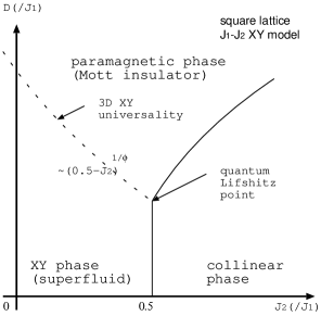
Figure 1: A schematic ground-state phase diagram Dutta98 is presented for the $S=1$ square-lattice $J_{1}$-$J_{2}$ $XY$ model with the single-ion anisotropy $D$ (1). The limiting cases of $D=0$ Bishop08 and $J_{2}=0$ Pires11 have been investigated in depth. For large $D$, the paramagnetic phase is realized. In the small-$D$ regime, the $XY$ and collinear phases appear, as the second-neighbor interaction $J_{2}$ changes. The dashed (solid) line stands for the continuous (discontinuous) phase transition Dutta98 . The $XY$-paramagnetic phase boundary should belong to the 3D-$XY$ universality class Roscilde07 , and its end-point singularity at $J_{2}=0.5$ is our concern; the power-law behavior of the phase boundary (2) is characterized by the crossover critical exponent $\phi$ Riedel69 ; Pfeuty74 . In the boson language Roscilde07 , the $XY$ (paramagnetic) phase is interpreted as the superfluid (Mott insulator) phase.

A notable feature of the quantum Lifshitz criticality Dutta98 ; Hornreich75 ; Dutta97 ; Diehl00 ; Diehl01 ; Leite03 ; Mergulhao98 ; Mergulhao99 is that the correlation-length critical exponents, $\nu_{\perp}$ and $\nu_{\parallel}$, for the real-space and imaginary-time directions, respectively, are not identical. Because of the magnetic frustration within the real-space spin configuration, the correlation lengths for the real-space $\xi$ and imaginary-time $\xi_{\tau}$ directions diverge independently as

$$\xi\sim|D-D_{c}|^{-\nu_{\perp}}\ {\rm and}\ \xi_{\tau}(\sim\Delta E^{-1})\sim|D-D_{c}|^{-\nu_{\parallel}},$$ (3)

respectively, with the energy gap $\Delta E$ at the quantum Lifshitz point, $J_{2}=0.5$. The anisotropy is indexed quantitatively by the dynamical critical exponent

$$z=\nu_{\parallel}/\nu_{\perp}.$$ (4)

In the exact-diagonalization approach, we do not have to manage the finite-size scaling of the imaginary-time sector, because the ratio $\xi_{\tau}/\beta\to 0$ ($\beta$: the inverse temperature) vanishes a priori at the ground state, $\beta\to\infty$; note that the ground state is directly accessible via the exact diagonalization scheme. Thus, we are able to concentrate on the finite-size scaling of the real-space sector, and significant simplification is attained even for $z\neq 1$.

The character of the $J_{2}$-driven phase transition depends on the magnitude of the constituent spins, $S$. As shown in Fig. 1, a direct $XY$-collinear phase transition occurs for $S=1$ Bishop08 , whereas an intermediate phase appears around $J_{2}\approx 0.5$ as for the spin-half ($S=1/2$) magnet Bishop08b ; in the case of the easy-axis $XXZ$ magnet, the appearance of such an intermediate phase remains controversial Oitmaa20 ; Kalz11 . In fact, as mentioned above, the kinetic frustration leads to a variety of super-solid phases for the hard-core ($S=1/2$) Chen17 ; Tu20 and soft-core ($S=1$) Dong17 boson models. Here, we focus our attention on the soft-core-boson case, namely, the $S=1$ $XY$ magnet Bishop08 , and show that the end-point singularity of the super-fluid-insulator phase boundary is under the reign of the above-mentioned critical exponents, $\phi$ and $\nu_{\parallel,\perp}$.

The rest of this paper is organized as follows. In Sec. 2, the numerical results are presented. The finite-size scaling theory for the fidelity susceptibility is outlined prior to presenting the simulation data. In Sec. 3, we present the summary and discussions.

2 Numerical results

In this section, we present the numerical results for the $S=1$ $J_{1}$-$J_{2}$ $XY$ magnet (1). We employed the Lanczos method for the cluster with $N\leq 5^{2}$ spins. To allocate the memory space, the symmetries possessed by the Hamiltonian (1), such as the translational invariance, are incorporated into the representation of the spin configuration Sandwick10 so that the $N=5^{2}$ spins can be tractable Nishiyama21 ; Nishiyama22 . Thereby, we evaluated the fidelity susceptibility Quan06 ; Zanardi06 ; HQZhou08 ; Yu09 ; You11

$$\chi_{F}=-\frac{1}{N}\partial_{\Delta D}^{2}F(D,D+\Delta D)|_{\Delta D=0},$$ (5)

with the fidelity $F(D,D+\Delta D)=|\langle D|D+\Delta D\rangle|$ Uhlmann76 ; Jozsa94 ; Peres84 ; Gorin06 , The fidelity $F$ is readily accessible via the exact diagonalization scheme, because the ground state $|D\rangle$ with the single-ion anisotropy $D$ is explicitly evaluated. Actually, the finite difference method yields the second derivative $\partial_{\Delta D}^{2}F|_{\Delta D=0}$ reliably, because the leading terms, i.e., $F|_{\Delta D=0}=1$ and $\partial_{\Delta D}F|_{\Delta D=0}=0$, are the constant values by definition.

To begin with, we outline the finite-size-scaling theory for the fidelity susceptibility $\chi_{F}$ (5); the crossover-scaling theory is explained afterward. The fidelity susceptibility $\chi_{F}$ obeys the scaling formula Albuquerque10

$$\chi_{F}=L^{x}f\left((D-D_{c})L^{1/\nu}\right),$$ (6)

with the system size $L(=\sqrt{N})$, scaling dimension $x=\alpha_{F}/\nu$, critical point $D_{c}$, and a certain scaling function $f$. Here, the indices, $\alpha_{F}$ and $\nu$, are the fidelity-susceptibility and correlation-length critical exponents, respectively. That is, the fidelity susceptibility and correlation length diverge as $\chi_{F}\sim|D-D_{c}|^{-\alpha_{F}}$ and $\xi\sim|D-D_{c}|^{-\nu}$, respectively. These indices satisfy the scaling relation Albuquerque10

$$\alpha_{F}=\alpha+z\nu.$$ (7)

with the critical exponent $\alpha$ of the specific heat, $C\sim|D-D_{c}|^{-\alpha}$. Therefore, fidelity-susceptibility’s scaling dimension $x=\alpha_{F}/\nu$ reduces to

$$x(=\alpha_{F}/\nu)=2/\nu-2,$$ (8)

from the hyper-scaling relation Albuquerque10

$$\alpha=2-(d+z)\nu,$$ (9)

with the real-space dimensionality $d=2$. Notably, the dynamical critical exponent $z$ cancels out in the final expression, Eq. (8). Owing to this cancellation, the $\chi_{F}$-mediated scaling analysis of criticality retrieves a substantial simplification.

2.1 Finite-size-scaling analysis with the fixed $J_{2}$: $\chi_{F}$ approach

In this section, we investigate the criticality of the $XY$-paramagnetic phase transition via the fidelity susceptibility $\chi_{F}$ (5) with the fixed next-nearest-neighbor interaction, $J_{2}=-1/32$, for which a preceeding result Moura14 is available.

In Fig. 2, we present the fidelity susceptibility $\chi_{F}$ (5) for various single-ion anisotropy $D$ and system sizes, ($+$) $L=3$ ($\times$) $4$ and ($*$) $5$, with the fixed $J_{2}=-1/32$. The fidelity susceptibility shows a notable peak, which indicates an onset of the $XY$-paramagnetic phase transition around $D=D_{c}\approx 5$. The paramagnetic phase extends for large $D>D_{c}$, whereas the $XY$ phase is realized for small $D<D_{c}$ Moura14 . In the boson language Roscilde07 , the single-ion anisotropy $D$ is regarded as the on-site Coulomb repulsion. Hence, the interaction $D$ induces the Mott insulator phase from the super-fluid phase. Afterward, we show the energy gap, which elucidates the character of each phase clearly.

Figure 2: The fidelity susceptibility $\chi_{F}$ (5) is plotted for various single-ion anisotropy $D$ and system sizes, ($+$) $L=3$, ($\times$) $4$, and ($*$) $5$, with the fixed $J_{2}=-1/32$, for which a preceding self-consistent-harmonic-approximation result Moura14 is available. The fidelity susceptibility exhibits a notable signature for the criticality at $D=D_{c}\approx 5$. The critical point $D_{c}$ separates the $XY$ ($D<D_{c}$) and paramagnetic ($D>D_{c}$) phases.

In order to appreciate the critical point $D_{c}$ in the thermodynamic limit, in Fig. 3, we present the approximate critical point $D_{c}^{*}(L)$ for $1/L^{1/\nu}$ with the 3D-$XY$ correlation-length critical exponent $\nu=0.6717$ Campostrini06 ; Burovski06 . Here, the approximate critical point $D_{c}^{*}(L)$ denotes the peak position

$$\partial_{D}\chi_{F}|_{D=D_{c}^{*}(L)}=0,$$ (10)

of $\chi_{F}(L)$ for each system size $L$. The abscissa scale $1/L^{1/\nu}$ comes from the definition of $\nu$, i.e., $\xi\sim|D-D_{c}|^{-\nu}$, and the finite-size-scaling hypothesis, $\xi\sim L$; therefore, the data points in Fig. 3 should align. The least-squares fit to these data yields an estimate $D_{c}=5.90(4)$ for the critical point in the thermodynamic limit $L\to\infty$. As a reference, we also made an alternative extrapolation for the $L=4$-$5$ pair, and arrived at $D_{c}=5.82$; the deviation from the former one, $\approx 0.08$, appears to dominate the least-squares-fit error $\approx 0.04$, Hence, regarding the deviation $0.08$ as a possible systematic error, we estimate the critical point

$$D_{c}=5.90(8).$$ (11)

As a comparison, in Table 1, we present the preceding result Moura14 for the two-dimensional $S=1$ $XY$ ferromagnet with the algebraically decaying interactions, $1/r^{10}$ ($r$: distance between spins), by means of the self-consistent harmonic approximation (SCHA) method. According to this study, the critical point $D_{c}=6.14$ was obtained; this value was read off from Fig. 1 of Ref. Moura14 . Thus, the slight discrepancy between this and ours can be attributed to the further neighbor ($r>\sqrt{2}$) interactions. Additionally, the SCHA approach is not very adequate to treat the ground-state phase transition, and it always overestimates the critical point, $D_{c}$.

Figure 3: The approximate critical point $D_{c}^{*}(L)$ (10) is plotted for $1/L^{1/\nu}$ with $J_{2}=-1/32$. Here, the correlation-length critical exponent $\nu$ is set to the value of the 3D-$XY$-universality class, $\nu=0.6717$ Campostrini06 ; Burovski06 . The least-squares fit to these data yields an estimate $D_{c}=5.90(4)$ in the thermodynamic limit $L\to\infty$. A possible systematic error is considered in the text.

Table 1: The critical point $D_{c}$ has been estimated with the self-consistent-harmonic-approximation (SCHA) method Moura14 tor the $S=1$ $XY$ ferromagnet with the algebraically decaying interactions, $1/r^{10}$ ($r$: distance between spins); the result $D_{c}$ was read off from Fig.1 of Ref. Moura14 . The present exact-diagonalization (ED) simulation was performed for the $J_{1}$-$J_{2}$ model with $J_{2}=-1/32$. Therefore, the slight discrepancy can be attributed to the further neighbor ($r>\sqrt{2}$) interactions as well as the systematic deviation (overestimation) inherent in SCHA at the ground state.

Method	Model	$D_{c}(/J_{1})$
SCHA Moura14	algebraically decaying interactions $r^{-10}$	$6.14$
ED (this work)	second neighbor interaction $J_{2}/J_{1}=-\frac{1}{32}$	$5.90(8)$

As a cross-check, we examine $\chi_{F}$’s finite-size scaling behavior, based on the scaling formula (6). In Fig. 4, we present the finite-size-scaling plot, $(D-D_{c})L^{1/\nu}$ versus $L^{-x}\chi_{F}$, for various $D$ and system sizes, ($+$) $L=3$, ($\times$) $4$, and ($*$) $5$, with the fixed $J_{2}=-1/32$ and $x=2/\nu-2$ (8). Here, the scaling parameters are set to $D_{c}=5.90$ (11) and $\nu=0.6717$ for the 3D-$XY$ universality class Campostrini06 ; Burovski06 . We stress that no ad hoc adjustable parameter is undertaken. The scaled data seem to fall into the scaling curve satisfactorily, confirming the validity of the $\chi_{F}$-mediated analysis of the criticality.

Figure 4: The scaling plot, $(D-D_{c})L^{1/\nu}$ versus $L^{-x}\chi_{F}$, is presented for various $D$ and system sizes, ($+$) $L=3$, ($\times$) $4$, and ($*$) $5$, with the fixed $J_{2}=-1/32$ and $x=2/\nu-2$ (8). Here, the scaling parameters are set to $D_{c}=5.90$ (11), and $\nu=0.6717$ for the 3D-$XY$ universality class Campostrini06 ; Burovski06 . Hence, no ad hoc adjustable parameter is undertaken. The scaled data seem to fall into a scaling curve satisfactorily.

Last, we address a remark. The singularity of the fidelity susceptibility, $x=\alpha_{F}/\nu$ (8), is larger than that of the specific heat, $\alpha/\nu$, as the scaling relation (7) indicates. Such a feature is significant in the above finite-size-scaling analyses, because specific-heat’s index $\alpha$ is negative for the 3D-$XY$ universality class Campostrini06 ; Burovski06 . The fidelity susceptibility picks up the singularity out of the regular part rather sensitively. Hence, the scaling behavior is less influenced by the finite-size artifact Yu09 , as compared to the ordinary quantifiers such as the specific heat. Encouraged by this finding, we turn to the analysis of multi-criticality via the probe $\chi_{F}$.

2.2 Crossover-scaling analysis around $J_{2}\to 0.5^{-}$: $\chi_{F}$ approach

In this section, we explore the crossover-scaling behavior of the fidelity susceptibility $\chi_{F}$ (5) around $J_{2}=0.5$ in the context of the quantum Lifshitz point Dutta98 ; more specifically, we investigate how the phase boundary ends up at $J_{2}=0.5$. For that purpose, we have to extend the scaling formula (6) so as to include yet another scaling parameter, $0.5-J_{2}$ (distance from the multi-critical point), and an accompanying crossover exponent $\phi$. According to the crossover-scaling theory Riedel69 ; Pfeuty74 , the extended scaling formula should read

$$\chi_{F}=L^{\dot{x}}g\left((D-D_{c}(J_{2}))L^{1/\nu_{\perp}},(0.5-J_{2})L^{\phi/\nu_{\perp}}\right),$$ (12)

with the multi-critical scaling dimension $\dot{x}$, crossover exponent $\phi$, distance from the multi-critical point, $0.5-J_{2}$, and a certain scaling function $g$. As in Eq. (8), the multi-critical scaling dimension $\dot{x}$ is given by

$$\dot{x}(=\dot{\alpha}_{F}/\nu_{\perp})=2/\nu_{\perp}-2,$$ (13)

with the multi-critical fidelity susceptibility critical exponent $\dot{\alpha}_{F}$, i.e., $\chi_{F}\sim|D-D_{c}|^{-\dot{\alpha}_{F}}$ and the multi-critical correlation length critical exponent $\nu_{\perp}$ (3). Notably, the scaling dimension $\dot{x}=2/\nu_{\perp}-2$ (13) is not affected by $z$. The exponent $z$ is thus considered in the next section. As mentioned in Introduction, the crossover exponent $\phi$ is relevant to the algebraic singularity of the phase boundary, $D_{c}\sim(0.5-J_{2})^{1/\phi}$ (2). This relation immediately follows from the above scaling formula (12): Because the second argument of the scaling formula (12) is scale-invariant (dimensionless), the relation $(0.5-J_{2})^{1/\phi}\sim L^{-1/\nu_{\perp}}$ holds. The definition of $\nu_{\perp}$, i.e., $\xi\sim|D-D_{c}|^{-\nu_{\perp}}$ (3), and the scaling hypothesis, $L\sim\xi$, admit the desired expression, $D_{c}\sim(0.5-J_{2})^{1/\phi}$ (2).

We then apply the scaling theory (12) to the analysis of the simulation data. In Fig. 5, we present the crossover-scaling plot, $(D-D_{c}(J_{2}))L^{1/\nu_{\perp}}$ versus $L^{-\dot{x}}\chi_{F}$, for various $D$ and system sizes, ($+$) $L=3$, ($\times$) $4$, and ($*$) $5$, with the multi-critical scaling dimension $\dot{x}=2/\nu_{\perp}-2$ (13), and the critical point $D_{c}(J_{2})$ determined via the same scheme as that of Sec. 2.1. Here, the second argument of the crossover-scaling formula (12) fixed to $(J_{2}-0.5)L^{\phi/\nu_{\perp}}=0.72$ with the optimal values of the multi-critical indices, $\phi=0.6$ and $\nu_{\perp}=0.5$. In Fig. 5, we see that the crossover-scaled data collapse into a scaling curve. Actually, around the critical point, $(D-D_{c})L^{1/\nu_{\perp}}\approx 0$ (right-side slope), in particular, the data for $L=4$ ($\times$) and $5$ ($*$) are almost overlapping each other. Likewise, we made similar crossover-scaling analyses for other values of $\phi$ and $\nu_{\perp}$, and found that these indices lie within

$$\phi=0.60(15),$$ (14)

and

$$\nu_{\perp}=0.5(1),$$ (15)

respectively.

Figure 5: The crossover-scaling plot, $(D-D_{c}(J_{2}))L^{1/\nu_{\perp}}$ versus $L^{-\dot{x}}\chi_{F}$, is presented for various $D$ and system sizes, ($+$) $L=3$, ($\times$) $4$, and ($*$) $5$, with the fixed crossover exponent $\phi=0.6$, multi-critical correlation-length exponent $\nu_{\perp}=0.5$, and multi-critical scaling dimension $\dot{x}(=2/\nu_{\perp}-2)=2$ (13). The second argument of the crossover-scaling formula (16) is fixed to $(0.5-J_{2})L^{\phi/\nu_{\perp}}=0.72$. The $L=4$ ($\times$) and $5$ ($*$) data are almost overlapping each other.

We address a few remarks. First, the underlying mechanisms behind the scaling plots, Fig. 4 and 5, are not identical. Actually, the scaling dimensions of the former, $x\approx 0.98\dots$ (8), and the latter, $\dot{x}=2$ (13), are far apart. Therefore, the data collapse of the crossover-scaling plot in Fig. 5 is by no means accidental; actually, both $\phi$ and $\nu_{\perp}$ have to be tuned carefully. Last, the direct numerical simulation right at $J_{2}=0.5$ suffers from finite-size artifact due to the $J_{2}$-mediated precursor to the super-lattice structures (stripe patterns), which may conflict with the system size $L$. The crossover-scaling formula (12) provides an alternative route toward $J_{2}\to 0.5^{-}$ to attain smooth finite-size-scaling behaviors.

2.3 Crossover-scaling analysis around $J_{2}\to 0.5^{-}$: $\Delta E$ approach

In this section, we estimate the dynamical critical exponent $z$ (4) at the quantum Lifshitz point. For that purpose, we consider the energy gap $\Delta E$. The energy gap should obey the same crossover-scaling formula Riedel69 ; Pfeuty74 as that of $\chi_{F}$ (12)

$$\Delta E=L^{\dot{y}}h\left((D-D_{c}(J_{2}))L^{1/\nu_{\perp}},(0.5-J_{2})L^{\phi/\nu_{\perp}}\right),$$ (16)

with $\Delta E$’s multi-critical scaling dimension $\dot{y}$, and a certain scaling function $h$. The scaling dimension $\dot{y}$ is given by the dynamical critical exponent

$$\dot{y}=-z,$$ (17)

because of Eq. (3), (4) and the scaling hypothesis, $\xi\sim L$. Technically, the energy gap was evaluated by the expression

$$\Delta E=E_{0}(1)-E_{0}(0).$$ (18)

Here, the symbol $E_{0}(S^{z}_{tot})$ denotes the ground state energy within the Hilbert-space sector indexed by the total longitudinal magnetic moment $S^{z}_{tot}$. In the language boson, this quantity measures the energy cost due to the increment by one particle.

In Fig. 6, we present the crossover-scaling plot, $(D-D_{c}(J_{2}))L^{1/\nu_{\perp}}$ versus $L^{z}\Delta E$, for various $D$ and system sizes, ($+$) $L=3$, ($\times$) $4$, and ($*$) $5$, with an optimal value of the dynamical critical exponent $z=1.8$. Here, the second argument of the crossover-scaling formula (16) is fixed to $(0.5-J_{2})L^{\phi/\nu_{\perp}}=0.72$, as in Fig. 5. The scaling parameters, $\nu_{\perp}=0.5$ and $\phi=0.6$, are also taken from Fig. 5. In Fig. 6, the scaled data seem to collapse into a scaling curve satisfactorily. Such a feature confirm the validity of the crossover-scaling analysis of $\chi_{F}$ in Fig. 5. We made similar data analyses for other values of $z$, and conclude that the dynamical critical exponent lies within

$$z=1.8(2).$$ (19)

Note that for the ordinary phase transition including the 3D-$XY$ universality, the dynamical critical exponent should be $z=1$. Therefore, the value $z=1.8$ indicates that the multi-criticality at $J_{2}=0.5$ is characterized by the anisotropy between the real-time and imaginary-time subspaces. The dynamical critical exponent $z=1.8(2)$ [Eq. (19)] determines the correlation-length critical exponent $\nu_{\parallel}$ along the imaginary-time direction

$$\nu_{\parallel}=0.9(2),$$ (20)

through the relations, Eq. (3) and (4).

This is a good position to make a comparison between the preceeding field-theoretical result Diehl01 and ours. As mentioned in Introduction, the end-point singularity of the $XY$-paramagnetic phase boundary (multi-criticality) has been investigated in the context of the quantum Lifshitz point Dutta98 . The $\varepsilon$-expansion results up to O$(\varepsilon^{2})$ are reported in Ref. Diehl01 ; in these expressions, the parameters, frustrated subspace dimension $m$ and number of order-parameter’s components $N$, have to be set to $m=2$ and $N=2$, respectively, and the expansion parameter $\varepsilon$ has to be set to $\varepsilon=2$ because of the upper critical dimension $d^{*}=5$ Diehl01 . In Table 2, the raw $\varepsilon$-expansion results as well as the $[1:1]$ Padé approximants for the indices, $\nu_{\perp}$, $\nu_{\parallel}$, and $\phi$, are shown. These two results look alike except $\nu_{\parallel}$; the deviations between them may be regarded as indicators of uncertainty. Within the error margins, our results agree with those of the $\varepsilon$-expansion method. Specifically, as to $\phi$, our result supports the raw data. Hence, the end-point singularity for the $S=1$ $J_{1}$-$J_{2}$ $XY$ model (1) can be identified as the quantum Lifshitz critical point Dutta98 .

Figure 6: The crossover-scaling plot, $(D-D_{c}(J_{2}))L^{1/\nu_{\perp}}$ versus $L^{z}\Delta E$, is presented for various $D$ and system sizes, ($+$) $L=3$, ($\times$) $4$, and ($*$) $5$, with an optimal dynamical critical exponent $z=1.8$. The second argument of the crossover-scaling formula (16) is fixed to $(0.5-J_{2})L^{\phi/\nu_{\perp}}=0.72$. The indices $\nu_{\perp}=0.5$ and $\phi=0.6$ are the same as those of Fig. 5.

Table 2: The two-dimensional O$(2)$ quantum Lifshitz criticality Dutta98 has been investigated with the $\varepsilon$-expansion ($\varepsilon$ exp.) method up to O$(\varepsilon^{2})$ Diehl01 . The results for the multi-critical indices, $\nu_{\perp}$, $\nu_{\parallel}(=z\nu_{\perp})$, and $\phi$, as well as the $[1:1]$ Padé approximants are shown. The expansion parameter has to be set to $\varepsilon=2$ because of the upper critical dimension $d^{*}=5$ Diehl01 .

indices	O$(\varepsilon^{2})$ $\varepsilon$ exp. Diehl01	$[1:1]$ Padé	this work
$\nu_{\perp}$	$0.421$	$0.600$	$0.5(1)$
$\nu_{\parallel}$	$0.867$	$1.696$	$0.9(2)$
$\phi$	$0.661$	$0.763$	$0.60(15)$

Last, we address a remark. The $\Delta E$ data in Fig. 6 show that in the paramagnetic ($XY$) phase, $D>(<)D_{c}$, the energy gap opens (closes); note that the ordinate axis is scaled by $L^{z}$. Actually, as the formula (3) indicates, the gap opens almost linearly as

$$\Delta E(\sim|D-D_{c}|^{\nu_{\parallel}})\sim|D-D_{c}|^{0.9},$$ (21)

in the $D>D_{c}$ side. Hence, the energy gap captures the character of each phase clearly. In contrast, as shown in Fig. 5, the fidelity susceptibility is rather sensitive to the onset of the phase transition. The gapless excitation in the $XY$ phase corresponds to the Goldstone mode (spin wave), whereas the finite magnon mass indicates the paramagnetism. In the boson language, this finite magnon mass is interpreted as the Mott-insulator gap induced by the on-site Coulomb repulsion $D$; see the formula (18) for $\Delta E$.

3 Summary and discussions

The $S=1$ square-lattice $J_{1}$-$J_{2}$ $XY$ magnet with the single-ion anisotropy $D$ (1) was investigated with an emphasis on the end-point singularity of the $XY$-paramagnetic phase boundary toward $J_{2}\to 0.5^{-}$. To surmount the negative sign problem of the QMC method, we employed the exact diagonalization method, and as a probe to detect the criticality, we implemented the fidelity susceptibility $\chi_{F}$ (5). A benefit of the $\chi_{F}$-mediated approach is that the scaling dimension (8) is not affected by the dynamical critical exponent $z(\neq 1)$. As a demonstration, under the setting $J_{2}=-1/32$ Moura14 , the $D$-driven phase transition was analyzed via $\chi_{F}$. Based on the scaling formula (6), we confirmed that the $XY$-paramagnetic phase transition belongs to the 3D-$XY$ universality class rather clearly. Thereby, the $\chi_{F}$ data were cast into the crossover scaling formula (12) with the properly scaled distance from the multi-criticality, $0.5-J_{2}\sim L^{-\phi/\nu_{\perp}}$. As a result, the crossover exponent $\phi$ and the multi-critical correlation-length exponent $\nu_{\perp}$ are estimated as $\phi=0.60(15)$ [Eq. (14)] and $\nu_{\perp}=0.5(1)$ [Eq. (15)], respectively. Additionally, making the similar crossover-scaling analysis of the energy gap $\Delta E$, we obtained the dynamical critical exponent $z=1.8(2)$ [Eq. (19)]. As shown in Table 2, these critical indices agree with those of the quantum Lifshitz criticality Dutta98 ; Diehl01 within the error margins of both analyses.

Our result shows that the $XY$-paramagnetic phase boundary terminates at $J_{2}\to 0.5^{-}$, obeying the quantum-Lifshitz-point scenario. For the Ising counterpart, the similar conclusion was obtained with the extensive series-expansion analysis Oitmaa20 . As for the $XXZ$ case, intermediate phases are induced around the multi-critical point Kalz11 . Therefore, it would be tempting to consider how the above quantum Lifshitz criticality changes, as the extended interactions are turned on. This problem is left for the future study.

Data Availability Statement

My manuscript has no associated data.

Data will be made available on reasonable request.

References

- (1) S. Wessel and M. Troyer, Phys. Rev. Lett. 95 (2005) 127205.
- (2) D. Heidarian and K. Damle, Phys. Rev. Lett. 95 (2005) 127206.
- (3) J.-Y. Gan and J.-F. Gan, J. Phys. Soc. Jpn. 78 (2009) 094602.
- (4) S. R. Hassan, L. de Medici, and A.-M. S. Tremblay, Phys. Rev. B 76 (2007) 144420.
- (5) M. Boninsegni and N. Prokof’ev, Phys. Rev. Lett. 95 (2005) 237204.
- (6) M. Boninsegni and N. V. Prokof’ev, Rev. Mod. Phys. 84 (2012) 759.
- (7) T. Matsubara and H. Matsuda, Prog. Theor. Phys. 16 (1956) 569.
- (8) T. Roscilde and S. Haas, Phys. Rev. Lett. 99 (2007) 047205.
- (9) Y.-C. Chen and M.-F. Yang, J. Phys. Communications 1 (2017) 035009.
- (10) W.-L. Tu, H.-K. Wu and T. Suzuki, J. Phys.: Condens. Matter 32 (2020) 455401.
- (11) S.-J. Dong, W. Liu, X.-F. Zhou, G.-C. Guo, Z.-W. Zhou, Y.-J. Han, and L. He, Phys. Rev. B 96 (2017) 045119.
- (12) H. T. Quan, Z. Song, X. F. Liu, P. Zanardi, and C. P. Sun, Phys. Rev. Lett. 96 (2006) 140604.
- (13) P. Zanardi and N. Paunković, Phys. Rev. E 74 (2006) 031123.
- (14) H.-Q. Zhou, and J. P. Barjaktarevic̃, J. Phys. A: Math. Theor. 41 (2008) 412001.
- (15) W.-C. Yu, H.-M. Kwok, J. Cao, and S.-J. Gu, Phys. Rev. E 80 (2009) 021108.
- (16) W.-L. You and Y.-L. Dong, Phys. Rev. B 84 (2011) 174426.
- (17) A. Uhlmann, Rep. Math. Phys. 9 (1976) 273.
- (18) R. Jozsa, J. Mod. Opt. 41 (1994) 2315.
- (19) A. Peres, Phys. Rev. A 30 (1984) 1610.
- (20) T. Gorin, T. Prosen, T. H. Seligman, and M. Žnidarič, Phys. Rep. 435 (2006) 33.
- (21) A. F. Albuquerque, F. Alet, C. Sire, and S. Capponi, Phys. Rev. B 81 (2010) 064418.
- (22) M. Campostrini, M. Hasenbusch, A. Pelissetto, and E. Vicari, Phys. Rev. B 74, 144506 (2006).
- (23) E. Burovski, J. Machta, N. Prokof’ev, and B. Svistunov, Phys. Rev. B 74, 132502 (2006).
- (24) A. Dutta, J. K. Bhattacharjee and B. K. Chakrabarti, Eur. Phys. J. B 3 (1998) 97.
- (25) R. F. Bishop, P. H. Y. Li, R. Darradi, J. Richter and C. E. Campbell, J. Phys.: Condens. Matter 20 (2008) 415213.
- (26) A.S.T. Pires, J. Mag. Mag. Mat. 323 (2011) 1977.
- (27) E.K. Riedel and F. Wegner, Z. Phys. 225 (1969) 195.
- (28) P. Pfeuty, D. Jasnow, and M. E. Fisher, Phys. Rev. B 10 (1974) 2088.
- (29) R. M. Hornreich, M. Luban, and S. Shtrikman, Phys. Rev. Lett. 35 (1975) 1678.
- (30) A. Dutta, B. K. Chakrabarti, and J. K. Bhattacharjee, Phys. Rev. B 55 (1997) 5619.
- (31) H. W. Diehl and M. Shpot, Phys. Rev. B 62 (2000) 12338.
- (32) M. Shpot and H. W. Diehl, Nucl. Phys. B 612 (2001) 340.
- (33) M. M. Leite, Phys. Rev. B 67 (2003) 104415.
- (34) C. Mergulhão, Jr and C. E. I. Carneiro, Phys. Rev. B 58 (1998) 6047.
- (35) C. Mergulhão, Jr and C. E. I. Carneiro, Phys. Rev. B 59 (1999) 13954.
- (36) R. F. Bishop, P. H. Y. Li, R. Darradi, J. Schulenburg, and J. Richter, Phys. Rev. B 78 (2008) 054412.
- (37) J. Oitmaa, J. Phys. A: Mathematical and Theoretical 53 (2020) 085001.
- (38) A. Kalz, A. Honecker, S. Fuchs, and T. Pruschke, Phys. Rev. B 83 (2011) 174519; ibid. 84 (2011) 219902.
- (39) A. W. Sandvik, AIP Conf. Proc. 1297 (2010) 135.
- (40) Y. Nishiyama, J. Stat. Mech.: Theory and Experiment (2021) 033103.
- (41) Y. Nishiyama, J. Stat. Mech.: Theory and Experiment (2022) 033102.
- (42) A.R. Moura, J. Mag. Mag. Mat. 369 (2014) 62.