Confronting sound speed resonance with pulsar timing arrays

Abstract

The stochastic signal detected by pulsar timing arrays (PTAs) has raised great interest in understanding its physical origin. Assuming the signal is a cosmological gravitational-wave background produced by overly large primordial curvature perturbations, we investigate the sound speed resonance effect with an oscillatory behavior using the combined PTA data from NANOGrav 15-yr data set, PPTA DR3, and EPTA DR2. We find that the stochastic signal can be explained by the induced gravitational waves sourced by the sound speed resonance mechanism, with the oscillation frequency $f_{*}\in[1.51,4.90]\times 10^{-7}$Hz and the start time of oscillation $|\tau_{0}|\in[2.05,106]\times 10^{7}$s.

1 Introduction

Recently, four regional pulsar timing array (PTA) collaborations, including the North American Nanohertz Observatory for Gravitational Waves (NANOGrav) [1, 2], the Parkes PTA (PPTA) [3, 4], the European PTA (EPTA) [5, 6], and the Chinese PTA (CPTA) [7, 8], have announced the evidence of a stochastic signal consistent with the Hellings-Downs [9] spatial correlations in their latest data sets, pointing to the gravitational wave (GW) origin of this signal. Although many physical phenomena [10, 11, 12, 13, 14, 15, 16, 17] can be the source in the PTA frequency band, the exact source of this signal, whether originating from supermassive black hole binaries [18, 19, 20] or other cosmological sources [21, 22, 23, 24, 25, 26, 27, 28, 29, 30, 31, 32, 33, 34, 35, 36, 37, 38, 39, 40, 41, 42, 43, 44, 45, 46, 47], remains the subject of ongoing investigation.

Scalar-induced gravitational waves (SIGWs) [48, 49, 50, 51, 52, 53, 54, 55, 56, 57, 58, 59], accompanying the formation of primordial black holes (PBHs) [60, 61, 62, 63, 64, 65, 66, 67, 68, 69, 70, 71, 72, 73, 74, 75, 76, 77, 78, 79, 80, 81, 82, 83, 84, 85, 86, 87, 88, 89, 90, 91, 92, 93, 94, 95, 96, 97, 98, 99, 100, 101, 102], are a promising candidate for explaining this observed signal. The SIGWs are produced by the large curvature perturbations generated during the inflationary epoch. Recently, a novel mechanism for PBH formation and the production of SIGWs, known as sound speed resonance (SSR), was proposed in [103, 104, 105, 106, 107]. The SSR mechanism involves the presence of an oscillating square of the sound speed, which gives rise to a nonperturbative parametric amplification of specific perturbation modes during the inflationary epoch. Consequently, the power spectrum of primordial curvature perturbations exhibits some pronounced peaks at small scales, while maintaining near-scale invariance on larger scales, consistent with predictions from inflationary cosmology. It is noteworthy that this novel mechanism predicts the existence of several narrow peaks in the power spectrum of primordial curvature perturbations at smaller scales. Additionally, in accordance with the second-order cosmological perturbation theory, the enhanced primordial curvature perturbations from SSR mechanism are expected to induce significant GW signals.

In this work, assuming that the signal detected by PTAs originates from SIGWs, we jointly use the NANOGrav 15-yr data set, PPTA DR3, and EPTA DR2 to constrain the SSR model. In particular, we aim to explore whether the PTA signal is consistent with the SSR mechanism and also constrain the parameter space of SSR model. The rest of the paper is organized as follows. In Section 2, we provide an overview of the SSR model, focusing on the generation of primordial curvature perturbations. In Section 3, we introduce the energy density of SIGWs and PBH production. In Section 4, we describe the methodology for data analyses and present the results obtained from the latest PTA data sets. Finally, we make the conclusions in Section 5.

2 Sound speed resonance

In our paper, we will briefly review the mechanisms underlying SSR. To begin, we introduce the variable $u$, defined as $u\equiv z\zeta$, where $z\equiv\sqrt{2\epsilon}a/c_{s}$. Here, $a$ denotes the scale factor, $c_{s}$ represents the sound speed, and $\epsilon$ is the slow-roll parameter defined as $\epsilon\equiv-\dot{H}/H^{2}$. Additionally, $\zeta$ represents the comoving curvature perturbation, which remains invariant in the gauge. Considering the perturbation of Einstein equations, the Fourier mode of the variable $u$ satisfies the following equation [108, 109]

$$u^{\prime\prime}_{k}+\left(c_{s}^{2}k^{2}-\frac{z^{\prime\prime}}{z}\right)u_{k}=0,$$ (2.1)

where the prime denotes a derivative with respect to the conformal time $\tau$. In the SSR model, the oscillating sound speed is defined as follows [103]

$$c_{s}^{2}=\left\{\begin{aligned} &1,&\tau<\tau_{0},\\ &1-2\xi\left[1-\cos\left(2k_{*}\tau\right)\right],&\tau>\tau_{0},\end{aligned}\right.$$ (2.2)

where $\xi$ represents the amplitude of the oscillation, $k_{*}$ corresponds to the oscillation frequency, $\tau_{0}$ is the start time of oscillation. The oscillating sound speed can be realized within the effective field theory of inflation [110, 111]. For instance, in the multi-field inflation model, the sound speed is given by $c_{s}^{2}=(1+4\eta_{\perp}^{2}H^{2}/M_{0}^{2})^{-1}$. Here, $M_{0}$ has the dimension of mass and $\eta_{\perp}=V_{N}/(\dot{\phi_{0}}H)$, where $\phi_{0}$ and $V_{N}$ are related to the background inflatons and the potential, respectively [110]. Consequently, if there are oscillations in the potential of the inflation model, the oscillating sound speed in Eq. (2.2) can be obtained.

It is important to ensure that $c_{s}^{2}\geq 0$, which imposes the condition $\xi<1/4$. Additionally, $k_{*}\tau_{0}$ is chosen to be a multiple of $\pi$ to ensure a smooth transition of the sound speed from its constant value to the oscillating regime. As a result, the effective mass during the oscillation period can be simplified as

$$\frac{z^{\prime\prime}}{z}=\frac{2}{\tau^{2}}-\frac{4\xi k_{*}}{\tau}\sin(2k_{*}\tau)+4\xi k_{*}^{2}\cos(2k_{*}\tau)+\mathcal{O}(\xi^{2}).$$ (2.3)

Focusing on the sub-Hubble radius situation where $|k_{*}\tau|\gg 1$, the effective mass simplifies to $z^{\prime\prime}/z=4\xi k_{*}^{2}\cos(2k_{*}\tau)$. The perturbation equation (2.1) can be rewritten as

$$\frac{d^{2}u_{k}}{dx^{2}}+\left(A_{k}-2q\cos 2x\right)u_{k}=0,$$ (2.4)

where we introduce the variable $x\equiv-k_{*}\tau$, $A_{k}=(1-2\xi)k^{2}/k_{*}^{2}$ and $q=(2-k^{2}/k_{*}^{2})\xi$. This equation resembles the Mathieu equation, which exhibits parametric instability within specific ranges of $k$. The resonance bands are located in narrow ranges around $k\simeq nk_{*}$, given that $\xi\ll 1$ and $|q|\ll 1$.

Let’s consider the first resonance band with $n=1$ as an example. During the onset of resonance, we set the initial value of $u_{k}$ to the Bunch-Davies vacuum as $u_{k}(\tau_{0})=e^{-ik\tau_{0}}/\sqrt{2k}$. For modes outside the resonance bands, $u_{k}$ remains approximately constant within the Hubble radius. However, for modes within the resonance bands, the behavior of $u_{k}$ inside the Hubble radius can be described by

$$u_{k}(\tau)\propto\exp(\xi k_{*}\tau/2).$$ (2.5)

Using $u\equiv z\zeta$ and Equation (2.5), the evolution of the comoving curvature perturbation for the $k_{*}$ mode can be approximated as

$$\zeta_{k_{*}}(\tau)\simeq\zeta_{k_{*}}(\tau_{0})e^{\xi k_{*}(\tau-\tau_{0})/2}\frac{\tau}{\tau_{0}}.$$ (2.6)

This approximation holds within the Hubble radius, where $\zeta_{k_{*}}(\tau_{0})=-H\tau_{0}/\sqrt{4\epsilon k_{*}}$, which is determined by the Bunch-Davies vacuum. When the mode crosses the Hubble radius at $\tau_{*}=-1/k_{*}$, the amplitude is enhanced to

$$\zeta_{k_{*}}\simeq\zeta_{k_{*}}(\tau_{0})\left(\frac{-1}{k_{*}\tau_{0}}\right)e^{-\xi k_{*}\tau_{0}/2}\simeq\frac{H}{\sqrt{4\epsilon k_{*}^{3}}}e^{-\xi k_{*}\tau_{0}/2}.$$ (2.7)

The power spectrum of the primordial curvature perturbation, denoted as $P_{\zeta}$, is defined as $P_{\zeta}\equiv k^{3}|\zeta_{k}|^{2}/(2\pi^{2})$. Here, the resonance frequency exhibits an exponential amplification. As a result, the complete power spectrum can be parametrized as

$$P_{\zeta}(k)=A_{s}\left(\frac{k}{k_{p}}\right)^{n_{s}-1}\left\{1+\frac{\xi k_{*}}{2}e^{-\xi k_{*}\tau_{0}}\left[\delta(k-k_{*})+\sum_{n=2}^{\infty}a_{n}\delta(k-nk_{*})\right]\right\},$$ (2.8)

where $A_{s}=H^{2}/(8\pi^{2}\epsilon)\simeq 2.2\times 10^{-9}$ represents the amplitude of the power spectrum as in the standard inflation, $n_{s}\simeq 0.965$ corresponds to the spectral index at the pivot scale $k_{p}\simeq 0.05~{}\text{Mpc}^{-1}$ [112], and $a_{n}\ll 1$ represents the amplitude of the $n$th peak relative to the first peak. The coefficient in front of the $\delta$-function is determined by using a triangle approximation to estimate the area of the peak. Throughout our paper, we only consider the second and third peaks which are located at $2k_{*}$ and $3k_{*}$, respectively, and ignore other higher order peaks. This choice is motivated by the fact that the amplitudes of the peaks at higher orders are exponentially suppressed. Therefore we truncated the series at $n=3$ to ease the computational burden.

3 SIGWs and PBHs

In this section, we will introduce the formalism of SIGWs and PBHs. In the Newtonian gauge, the perturbed metric can be expressed as

$$ds^{2}=a^{2}(\tau)\left\{-(1+2\Phi)d\tau^{2}+\left[(1-2\Phi)\delta_{ij}+\frac{1}{2}h_{ij}\right]dx^{i}dx^{j}\right\},$$ (3.1)

where $\Phi$ represents the Bardeen potential, and $h_{ij}$ represents the tensor perturbations. Here, we neglect the effects of first-order gravitational waves, vector perturbations, and anisotropic stress, as previous studies ([49, 113, 114]) have demonstrated that their contributions are small. According to the Einstein field equations, the tensor perturbations in Fourier space can be written as [48, 49]

$$h^{\prime\prime}_{\bm{k}}+2\mathcal{H}h^{\prime}_{\bm{k}}+k^{2}h_{\bm{k}}=4S_{\bm{k}},$$ (3.2)

where $\mathcal{H}\equiv a^{\prime}/a$ is the comoving Hubble parameter, and $S_{\bm{k}}$ represents the source term given by

$$S_{\bm{k}}=\int\frac{d^{3}\bm{p}}{(2\pi)^{3/2}}e_{ij}(\bm{k})p^{i}p^{j}\left[3\Phi_{\bm{p}}\Phi_{\bm{k}-\bm{p}}+\mathcal{H}^{-1}\left(\Phi’_{\bm{p}}\Phi_{\bm{k}-\bm{p}}+\Phi_{\bm{p}}\Phi’_{\bm{k}-\bm{p}}\right)+\mathcal{H}^{-2}\Phi’_{\bm{p}}\Phi’_{\bm{k}-\bm{p}}\right].$$ (3.3)

The Bardeen potential in the Fourier space, denoted as $\Phi_{\bm{k}}$ , is related to the primordial curvature perturbations $\zeta_{\bm{k}}$ as $\Phi_{\bm{k}}=2/3~{}\zeta_{\bm{k}}$. The solution for tensor perturbations is given by

$$h_{\bm{k}}(\tau)=\frac{4}{a(\tau)}\int^{\tau}d\tau’g_{\bm{k}}(\tau,\tau’)a(\tau’)S_{\bm{k}}(\tau’),$$ (3.4)

where the Green function is defined as

$$g_{\bm{k}}(\tau,\tau^{\prime})=\frac{\sin\left[k(\tau-\tau^{\prime})\right]}{k}.$$ (3.5)

The power spectrum of tensor perturbations is given by:

$$\langle h_{\bm{k}}(\tau)h_{\bm{k}^{\prime}}(\tau)\rangle=\frac{2\pi^{2}}{k^{3}}\delta^{3}(\bm{k}+\bm{k}^{\prime})\mathcal{P}_{h}(k,\tau).$$ (3.6)

Hence, the power spectrum of tensor perturbations can be expressed as [48, 49, 53, 115]

$$\mathcal{P}_{h}(k,\tau)=4\int_{0}^{\infty}dv\int_{|1-v|}^{1+v}du\left[\frac{4v^{2}-\left(1-u^{2}+v^{2}\right)^{2}}{4uv}\right]^{2}I_{RD}^{2}(u,v)\mathcal{P}_{\zeta}(kv)\mathcal{P}_{\zeta}(ku),$$ (3.7)

where $u=|\bm{k}-\bm{p}|/k$, $v=p/k$, and $I_{RD}$ is the integral kernel. In the study of SGWBs, their characterization often involves quantifying the energy density per logarithmic frequency interval relative to the critical density $\rho_{c}(\tau)$, which is expressed as:

$$\Omega_{\mathrm{GW}}(k,\tau)\equiv\frac{1}{\rho_{c}(\tau)}\frac{\mathrm{d}\rho_{\mathrm{GW}}(k,\tau)}{\mathrm{d}\ln k}=\frac{k^{3}}{48\pi^{2}}\left(\frac{k}{\mathcal{H}}\right)^{2}\overline{\left\langle\left|h_{\bm{k}}(\tau)\right|^{2}\right\rangle},$$ (3.8)

Here, the term $\overline{\left\langle\left|h_{\bm{k}}(\tau)\right|^{2}\right\rangle}$ represents an average over a few wavelengths. During the radiation-dominated era, gravitational waves are generated by curvature perturbations. The density parameter of gravitational waves at the matter-radiation equality epoch is denoted as $\Omega_{\mathrm{GW}}(k)=\Omega_{\mathrm{GW}}(k,\tau\rightarrow\infty)$. Therefore, the energy density of GWs can be expressed as [115]

$$\Omega_{\mathrm{GW}}(k)=\int_{0}^{\infty}\mathrm{d}v\int_{|1-v|}^{|1+v|}\mathrm{d}u\mathcal{T}(u,v){P}_{\zeta}(vk){P}_{\zeta}(uk),$$ (3.9)

with

$$\mathcal{T}(u,v)=\frac{3}{1024v^{8}u^{8}}\left[4v^{2}-\left(v^{2}-u^{2}+1\right)^{2}\right]^{2}\left(v^{2}+u^{2}-3\right)^{2}$$ (3.10)

$$\times\left\{\left[\left(v^{2}+u^{2}-3\right)\ln\left(\left|\frac{3-(v+u)^{2}}{3-(v-u)^{2}}\right|\right)-4vu\right]^{2}+\pi^{2}\left(v^{2}+u^{2}-3\right)^{2}\Theta(v+u-\sqrt{3})\right\}.$$

Here, $\Theta$ is the Heaviside theta function. By employing the relationship between the wave number $k$ and frequency $f$, $k=2\pi f$, we can derive the energy density fraction spectrum of SIGWs at the present time,

$$\Omega_{\mathrm{GW},0}(f)=\Omega_{\mathrm{r},0}\left[\frac{g_{*,r}(T)}{g_{*,r}\left(T_{\mathrm{eq}}\right)}\right]\left[\frac{g_{*,s}\left(T_{\mathrm{eq}}\right)}{g_{*,s}(T)}\right]^{\frac{4}{3}}\Omega_{\mathrm{GW}}(k),$$ (3.11)

where $g_{*,s}$ and $g_{*,r}$ are the effective degrees of freedom for entropy density and radiation, and $\Omega_{r,0}$ denotes the present energy density fraction of radiation.

PBHs are produced from gravitational collapse when the density contrast $\delta\rho/\rho$ exceeds a critical threshold $\delta_{c}$ within Hubble patches. The exact value of $\delta_{c}$ depends on the equation of state parameter $w$ and the propagation speed $c_{s}^{2}$  [60, 61, 62, 116, 117, 118, 119, 120, 121, 122]. In a cautious estimation, we adopt Carr’s criterion in the uniform Hubble slice [117], which can be translated to the comoving slice as [86]

$$\delta_{c}\simeq\frac{3(1+w)}{5+3w}c_{s}^{2}.$$ (3.12)

The rationale for our selection of $\delta_{c}$ is justified by the fact that the fluctuations of the scalar field propagate at the speed of sound squared, making PBH formation more challenging than in an adiabatic perfect fluid. Thus, we adopt the upper limit of the density threshold from Ref. [121]. When $\xi\ll 1$, $c_{s}^{2}$ oscillates from $1-4\xi$ to $1$, which is nearly a constant. Therefore, in SSR model and the radiation-dominated era, $\delta_{c}\approx 2/3$, which can alleviate the tension of PBH overproduction. The PBH abundance is highly sensitive to the power spectrum, with the first band (n = 1) experiencing much greater enhancement than subsequent harmonic bands. Consequently, in the PBH abundance calculation, our focus is solely on the resonated modes around $k_{*}$. The relation of PBH mass $M$ and wavenumber $k$ is given by

$$k\approx\frac{1.7\times 10^{7}}{\mathrm{Mpc}}\left(\frac{M_{\odot}}{M}\right)^{1/2}\left(\frac{\gamma}{0.2}\right)^{1/2}\left(\frac{g_{*,r}\left(T\left(M\right)\right)}{106.75}\right)^{1/4}\left(\frac{g_{*,s}\left(T\left(M\right)\right)}{106.75}\right)^{-1/3},$$ (3.13)

where $M_{\odot}$ is the solar mass and $\gamma\approx 0.2$ denotes the fraction of matter within the Hubble horizon that undergoes gravitational collapse, leading to the formation of PBHs.

The estimation of PBH abundance with mass $M(k_{*})$ typically involves defining $\beta(M)$ as the mass fraction of PBHs relative to the total energy density at the time of formation. This quantity can be expressed as an integration of the Gaussian distribution of perturbations

$$\beta(M)=\frac{\gamma}{2}\text{erfc}\left(\frac{\delta_{c}}{\sqrt{2}\sigma(M)}\right).$$ (3.14)

The quantity $\sigma(M)$ denoting the variance of the density perturbation smoothed over the mass scale of $M$, is estimated as

$$\sigma^{2}=\frac{16}{81}~{}\int_{0}^{\infty}\!\frac{\mathrm{d}q}{q}\,\left(\frac{q}{k}\right)^{4}\tilde{W}^{2}(q/k)T^{2}(q/k)\mathcal{P}_{\mathcal{R}}(q),$$ (3.15)

where the function $\tilde{W}(q/k)=\exp(-q^{2}/2k^{2})$ corresponds to the Gaussian window function, and $T(q/k)=3(\sin l-l\cos l)/l^{3}$ is the transfer function, with $l=q/(\sqrt{3}k)$. When the primordial scalar power spectrum exhibits a very sharp peak, it leads to a monochromatic mass function for the PBHs. The total abundance of PBHs in the dark matter at present can be defined as [123]

$$f_{\mathrm{PBH}}\equiv\frac{\Omega_{\mathrm{PBH}}}{\Omega_{\mathrm{CDM}}}=2.7\times 10^{8}\left(\frac{g_{*,r}}{10.75}\right)^{3/4}\left(\frac{g_{*,s}}{10.75}\right)^{-1}\left(\frac{M}{M_{\odot}}\right)^{-1/2}\beta(M),$$ (3.16)

where $\Omega_{\mathrm{CDM}}$ represents the density of cold dark matter.

Parameter	$\log_{10}(f_{*}/\mathrm{Hz})$	$\log_{10}\xi$	$\log_{10}(-\tau_{0}/\mathrm{s})$
Prior	${\mathcal{U}}(-9,-5)$	${\mathcal{U}}(-4,\log_{10}0.25)$	${\mathcal{U}}(5,12)$
NANOGrav result	$-5.85^{+0.77}_{-1.17}$	$-2.17^{+1.43}_{-1.62}$	$8.66^{+2.07}_{-1.81}$
PPTA result	$-5.83^{+0.74}_{-0.80}$	$-2.13^{+1.38}_{-1.64}$	$8.55^{+1.92}_{-1.70}$
EPTA result	$-6.86^{+1.57}_{-0.76}$	$-2.18^{+1.45}_{-1.60}$	$9.42^{+2.04}_{-2.00}$
Combined result	$-6.31^{+0.92}_{-0.51}$	$-2.20^{+1.43}_{-1.57}$	$9.03^{+1.82}_{-1.71}$

Table 1: Prior distributions and results for the model parameters. We present the results obtained from the NANOGrav 15-yr data set, the PPTA DR3, the EPTA DR2, and the combined data (NANOGrav+PPTA+EPTA), respectively. Here ${\mathcal{U}}$ denotes the uniform distribution. We quote each parameter’s median value and $90\%$ equal-tail credible interval.

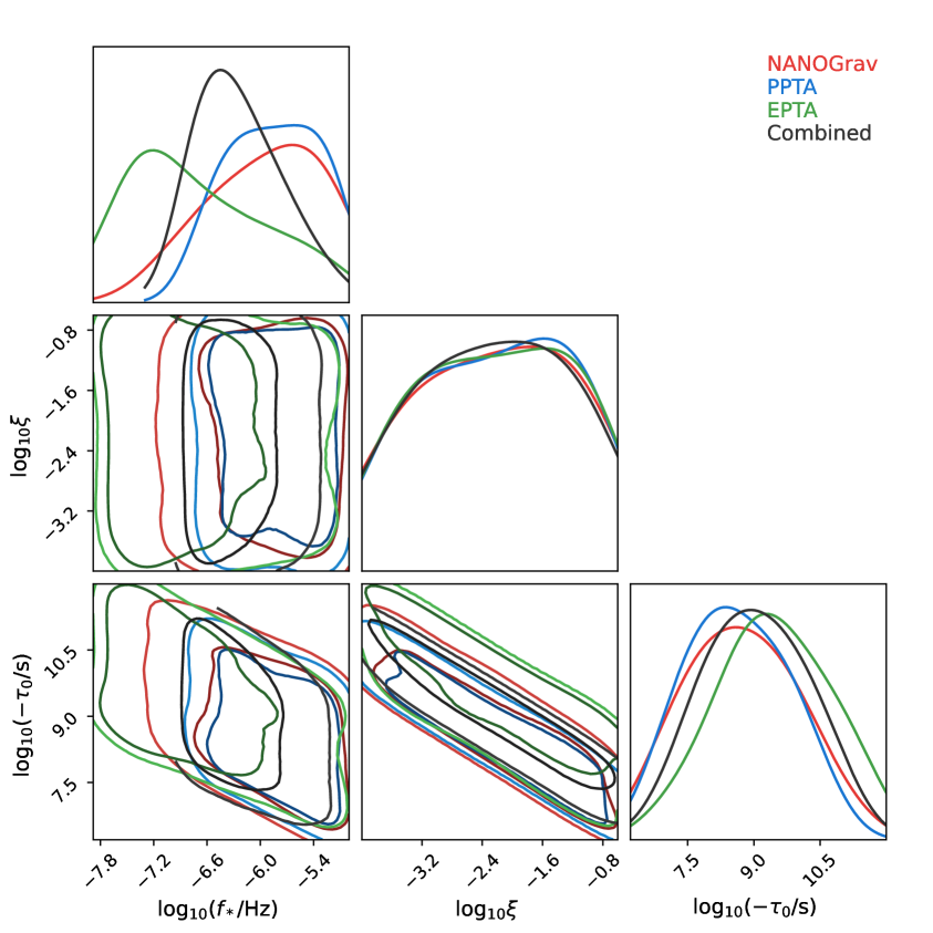
Figure 1: One and two-dimensional marginalized posteriors of the parameters obtained from the NANOGrav 15-yr data set, PPTA DR3, EPTA DR2, and the combined data (NANOGrav+PPTA+EPTA). The contours in the two-dimensional plot correspond to the $1\sigma$ and $2\sigma$ credible regions, respectively.

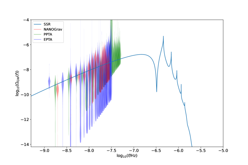
Figure 2: The energy density of SIGWs sourced by the SSR effect. We also show the energy density spectra derived from the free spectrum from NANOGrav 15-yr data set (red violins), PPTA DR3 (green violins), and EPTA DR2 (blue violins).

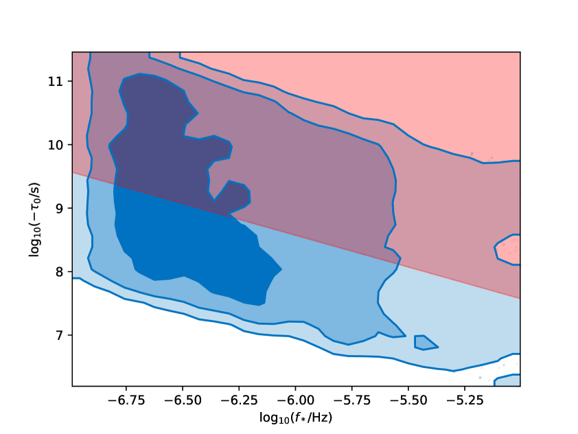
Figure 3: The two dimensional posteriors for the $\log_{10}(f_{*}/\mathrm{Hz})$ and $\log_{10}(-\tau_{0}/\mathrm{s})$ parameters shown in blue contours obtained from the combined data (NANOGrav+PPTA+EPTA). The red region is the excluded parameter space where $f_{\mathrm{PBH}}>1$ by fixing $\xi=0.01$.

4 Data analysis and results

Following [35, 40], we jointly use the NANOGrav 15-yr data set, the PPTA DR3, and the EPTA DR2 to estimate the model parameters. In this work, we use the free spectrum data obtained from each PTA with Hellings-Downs [9] spatial correlations. Given the time span $T_{\mathrm{obs}}$ of a PTA, the free-spectrum starts with the lowest frequency $1/T_{\mathrm{obs}}$. NANOGrav, PPTA, and EPTA use $14$ [1], $28$ [3], and $24$ [5] frequencies in searching for the GWB signal, respectively. In this work, we constrain the parameter space by considering the NANOGrav 15-yr data set, the PPTA DR3, the EPTA DR2, and the combined data (NANOGrav+PPTA+EPTA), respectively. In particular, the combined data consists $66$ frequencies for a free spectrum ranging from $1.28$ nHz to $49.1$ nHz. We note that although the simply combined data can improve the sensitivity in searching for SGWB signal, a proper way to combine the different PTA data sets should wait for the IPTA DR3 which is undergoing.

We use the free-spectrum time delay data released by each PTA. The time delay $d(f)$ is related to the power spectrum $S(f)$ by

$$d(f)=\sqrt{S(f)/T_{\mathrm{obs}}}.$$ (4.1)

We then obtain the characteristic strain, $h_{c}(f)$, by

$$h_{c}^{2}(f)=12\pi^{2}f^{3}S(f).$$ (4.2)

Finally, we can calculate the free-spectrum energy density as

$$\hat{\Omega}_{\mathrm{GW}}(f)=\frac{2\pi^{2}}{3H_{0}^{2}}f^{2}h_{c}^{2}(f)=\frac{8\pi^{4}}{H_{0}^{2}}T_{\mathrm{obs}}f^{5}d^{2}(f).$$ (4.3)

For each observed frequency, $f_{i}$, we can estimate the corresponding kernel density $\mathcal{L}_{i}$ given the posteriors of $\hat{\Omega}_{\mathrm{GW}}(f_{i})$ derived above. Therefore, the total likelihood is [35, 40]

$$\mathcal{L}(\Lambda)=\prod_{i=1}\mathcal{L}_{i}(\Omega_{\mathrm{GW}}(f_{i},\Lambda)),$$ (4.4)

where $\Lambda\equiv\{f_{*},\xi,\tau_{0}\}$ is the collection of the model parameters and $f_{*}=k_{*}/2\pi$. Table 1 summarizes the model parameters and their priors. Note that we sample in the log space for all these three parameters. In practice, we use dynesty [124] sampler wrapped in the Bilby [125, 126] package to explore the parameter space.

The posterior distributions of the model parameters, $\Lambda=\{f_{*},\xi,\tau_{0}\}$, are shown in Figure 1. The results for each model parameter with median and $90\%$ equal-tail credible interval obtained from different PTA data sets are summarized in Table 1. We see that the results derived from NANOGrav, PPTA, and EPTA are consistent with each other, and the combined data indeed have a better constraint on the parameters especially for the $f_{*}$ parameter. In what follows, we should focus on the results from the combined data. In particular, to explain the PTA signal, we obtain constraints on the oscillation frequency $\log_{10}(f_{*}/\mathrm{Hz})=-6.31^{+0.92}_{-0.51}$, the amplitude of the oscillation $\log_{10}\xi=-2.20^{+1.43}_{-1.57}$, and the start time of oscillation $\log_{10}(-\tau_{0}/s)=9.03^{+1.82}_{-1.71}$ with $90\%$ equal-tail uncertainties. Note that the SSR effect can alleviate the tension of PBH overproduction as shown in Figure 3. Because $c_{s}^{2}$ oscillates in the range of $[1-4\xi,1]$, it can be well approximated by $c_{s}^{2}\simeq 1$ when $\xi\ll 1$. Therefore, in the SSR model, we have $\delta_{c}\approx 2/3$ which is much larger than the value $\delta_{c}\approx 2/9$ as in an adiabatic perfect fluid where $c_{s}^{2}=w=1/3$ (see Eq. (3.12)), making PBH formation in the SSR model with $c_{s}^{2}\simeq 1$ more challenging than in an adiabatic perfect fluid where $c_{s}^{2}=w=1/3$. This effect has already been carefully discussed in Ref [127].

A representative of the SIGWs sourced by the SSR effect is shown in Figure 2, where five spikes appear in the energy density spectrum with $n=3$. A general feature of the SSR is that the number of spikes in the energy density spectrum is equal to $2n-1$ where $n$ is the number of peaks of the power spectrum defined in Eq. (2.8). Furthermore, the spikes of the energy density spectrum locate at $2f_{*}/\sqrt{3}$, $3f_{*}/\sqrt{3}$, $\cdots$, $2nf_{*}/\sqrt{3}$.

5 Conclusions

The stochastic signal detected by NANOGrav, PPTA, EPTA, and CPTA shows strong evidence of the Hellings-Downs spatial correlations, suggesting a GW origin of this signal. Assuming the signal is from the SIGWs induced by the primordial curvature perturbations, we constrain the SSR effect with combined PTA data from NANOGrav 15-yr data set, PPTA DR3, and EPTA DR2.

We find that the stochastic signal can be explained by the induced gravitational waves sourced by the SSR mechanism, with the oscillation frequency $f_{*}\in[1.52,4.67]\times 10^{-7}$Hz and the start time of oscillation $|\tau_{0}|\in[2.17,95.7]\times 10^{7}$s. The relatively high oscillation frequency $f_{*}$ implies that the oscillation structure from SSR effect lies out of the PTA frequency band and cannot be probed by PTA.

The resonating primordial curvature perturbations with an oscillatory feature in the sound speed of their propagation may be realized in the context of an effective field theory of inflation or by non-canonical models inspired by string theory [103]. We, therefore, expect the PTA data can also constrain the inflation models through the SSR mechanism. We leave it as future work.

References

- [1] NANOGrav collaboration, The NANOGrav 15 yr Data Set: Evidence for a Gravitational-wave Background, Astrophys. J. Lett. 951 (2023) L8 [2306.16213].
- [2] NANOGrav collaboration, The NANOGrav 15 yr Data Set: Observations and Timing of 68 Millisecond Pulsars, Astrophys. J. Lett. 951 (2023) L9 [2306.16217].
- [3] D.J. Reardon et al., Search for an Isotropic Gravitational-wave Background with the Parkes Pulsar Timing Array, Astrophys. J. Lett. 951 (2023) L6 [2306.16215].
- [4] A. Zic et al., The Parkes Pulsar Timing Array Third Data Release, 2306.16230.
- [5] J. Antoniadis et al., The second data release from the European Pulsar Timing Array III. Search for gravitational wave signals, 2306.16214.
- [6] J. Antoniadis et al., The second data release from the European Pulsar Timing Array I. The dataset and timing analysis, 2306.16224.
- [7] R. Nan, D. Li, C. Jin, Q. Wang, L. Zhu, W. Zhu et al., The Five-Hundred-Meter Aperture Spherical Radio Telescope (FAST) Project, Int. J. Mod. Phys. D 20 (2011) 989 [1105.3794].
- [8] H. Xu et al., Searching for the Nano-Hertz Stochastic Gravitational Wave Background with the Chinese Pulsar Timing Array Data Release I, Res. Astron. Astrophys. 23 (2023) 075024 [2306.16216].
- [9] R.w. Hellings and G.s. Downs, UPPER LIMITS ON THE ISOTROPIC GRAVITATIONAL RADIATION BACKGROUND FROM PULSAR TIMING ANALYSIS, Astrophys. J. Lett. 265 (1983) L39.
- [10] J. Li, Z.-C. Chen and Q.-G. Huang, Measuring the tilt of primordial gravitational-wave power spectrum from observations, Sci. China Phys. Mech. Astron. 62 (2019) 110421 [1907.09794].
- [11] Z.-C. Chen, C. Yuan and Q.-G. Huang, Non-tensorial gravitational wave background in NANOGrav 12.5-year data set, Sci. China Phys. Mech. Astron. 64 (2021) 120412 [2101.06869].
- [12] Y.-M. Wu, Z.-C. Chen and Q.-G. Huang, Constraining the Polarization of Gravitational Waves with the Parkes Pulsar Timing Array Second Data Release, Astrophys. J. 925 (2022) 37 [2108.10518].
- [13] Z.-C. Chen, Y.-M. Wu and Q.-G. Huang, Searching for isotropic stochastic gravitational-wave background in the international pulsar timing array second data release, Commun. Theor. Phys. 74 (2022) 105402 [2109.00296].
- [14] Z.-C. Chen, Y.-M. Wu and Q.-G. Huang, Search for the Gravitational-wave Background from Cosmic Strings with the Parkes Pulsar Timing Array Second Data Release, Astrophys. J. 936 (2022) 20 [2205.07194].
- [15] PPTA collaboration, Constraining ultralight vector dark matter with the Parkes Pulsar Timing Array second data release, Phys. Rev. D 106 (2022) L081101 [2210.03880].
- [16] Y.-M. Wu, Z.-C. Chen and Q.-G. Huang, Search for stochastic gravitational-wave background from massive gravity in the NANOGrav 12.5-year dataset, Phys. Rev. D 107 (2023) 042003 [2302.00229].
- [17] Y.-M. Wu, Z.-C. Chen and Q.-G. Huang, Pulsar timing residual induced by ultralight tensor dark matter, 2305.08091.
- [18] NANOGrav collaboration, The NANOGrav 15-year Data Set: Constraints on Supermassive Black Hole Binaries from the Gravitational Wave Background, 2306.16220.
- [19] J. Antoniadis et al., The second data release from the European Pulsar Timing Array: V. Implications for massive black holes, dark matter and the early Universe, 2306.16227.
- [20] Y.-C. Bi, Y.-M. Wu, Z.-C. Chen and Q.-G. Huang, Implications for the Supermassive Black Hole Binaries from the NANOGrav 15-year Data Set, 2307.00722.
- [21] S. Vagnozzi, Inflationary interpretation of the stochastic gravitational wave background signal detected by pulsar timing array experiments, 2306.16912.
- [22] C. Han, K.-P. Xie, J.M. Yang and M. Zhang, Self-interacting dark matter implied by nano-Hertz gravitational waves, 2306.16966.
- [23] Y. Li, C. Zhang, Z. Wang, M. Cui, Y.-L.S. Tsai, Q. Yuan et al., Primordial magnetic field as a common solution of nanohertz gravitational waves and Hubble tension, 2306.17124.
- [24] G. Franciolini, D. Racco and F. Rompineve, Footprints of the QCD Crossover on Cosmological Gravitational Waves at Pulsar Timing Arrays, 2306.17136.
- [25] Z.-Q. Shen, G.-W. Yuan, Y.-Y. Wang and Y.-Z. Wang, Dark Matter Spike surrounding Supermassive Black Holes Binary and the nanohertz Stochastic Gravitational Wave Background, 2306.17143.
- [26] N. Kitajima, J. Lee, K. Murai, F. Takahashi and W. Yin, Nanohertz Gravitational Waves from Axion Domain Walls Coupled to QCD, 2306.17146.
- [27] G. Franciolini, A. Iovino, Junior., V. Vaskonen and H. Veermae, The recent gravitational wave observation by pulsar timing arrays and primordial black holes: the importance of non-gaussianities, 2306.17149.
- [28] A. Addazi, Y.-F. Cai, A. Marciano and L. Visinelli, Have pulsar timing array methods detected a cosmological phase transition?, 2306.17205.
- [29] Y.-F. Cai, X.-C. He, X. Ma, S.-F. Yan and G.-W. Yuan, Limits on scalar-induced gravitational waves from the stochastic background by pulsar timing array observations, 2306.17822.
- [30] K. Inomata, K. Kohri and T. Terada, The Detected Stochastic Gravitational Waves and Sub-Solar Primordial Black Holes, 2306.17834.
- [31] S. Wang, Z.-C. Zhao, J.-P. Li and Q.-H. Zhu, Exploring the Implications of 2023 Pulsar Timing Array Datasets for Scalar-Induced Gravitational Waves and Primordial Black Holes, 2307.00572.
- [32] K. Murai and W. Yin, A Novel Probe of Supersymmetry in Light of Nanohertz Gravitational Waves, 2307.00628.
- [33] S.-P. Li and K.-P. Xie, A collider test of nano-Hertz gravitational waves from pulsar timing arrays, 2307.01086.
- [34] L.A. Anchordoqui, I. Antoniadis and D. Lust, Fuzzy Dark Matter, the Dark Dimension, and the Pulsar Timing Array Signal, 2307.01100.
- [35] L. Liu, Z.-C. Chen and Q.-G. Huang, Implications for the non-Gaussianity of curvature perturbation from pulsar timing arrays, 2307.01102.
- [36] K.T. Abe and Y. Tada, Translating nano-Hertz gravitational wave background into primordial perturbations taking account of the cosmological QCD phase transition, 2307.01653.
- [37] T. Ghosh, A. Ghoshal, H.-K. Guo, F. Hajkarim, S.F. King, K. Sinha et al., Did we hear the sound of the Universe boiling? Analysis using the full fluid velocity profiles and NANOGrav 15-year data, 2307.02259.
- [38] D.G. Figueroa, M. Pieroni, A. Ricciardone and P. Simakachorn, Cosmological Background Interpretation of Pulsar Timing Array Data, 2307.02399.
- [39] Z. Yi, Q. Gao, Y. Gong, Y. Wang and F. Zhang, The waveform of the scalar induced gravitational waves in light of Pulsar Timing Array data, 2307.02467.
- [40] Y.-M. Wu, Z.-C. Chen and Q.-G. Huang, Cosmological Interpretation for the Stochastic Signal in Pulsar Timing Arrays, 2307.03141.
- [41] X.-F. Li, Probing the high temperature symmetry breaking with gravitational waves from domain walls, 2307.03163.
- [42] M. Geller, S. Ghosh, S. Lu and Y. Tsai, Challenges in Interpreting the NANOGrav 15-Year Data Set as Early Universe Gravitational Waves Produced by ALP Induced Instability, 2307.03724.
- [43] Z.-Q. You, Z. Yi and Y. Wu, Constraints on primordial curvature power spectrum with pulsar timing arrays, 2307.04419.
- [44] S. Antusch, K. Hinze, S. Saad and J. Steiner, Singling out SO(10) GUT models using recent PTA results, 2307.04595.
- [45] G. Ye and A. Silvestri, Can gravitational wave background feel wiggles in spacetime?, 2307.05455.
- [46] S.A. Hosseini Mansoori, F. Felegray, A. Talebian and M. Sami, PBHs and GWs from -inflation and NANOGrav 15-year data, 2307.06757.
- [47] L. Liu, Z.-C. Chen and Q.-G. Huang, Probing the equation of state of the early Universe with pulsar timing arrays, 2307.14911.
- [48] K.N. Ananda, C. Clarkson and D. Wands, The Cosmological gravitational wave background from primordial density perturbations, Phys. Rev. D 75 (2007) 123518 [gr-qc/0612013].
- [49] D. Baumann, P.J. Steinhardt, K. Takahashi and K. Ichiki, Gravitational Wave Spectrum Induced by Primordial Scalar Perturbations, Phys. Rev. D 76 (2007) 084019 [hep-th/0703290].
- [50] J. Garcia-Bellido, M. Peloso and C. Unal, Gravitational waves at interferometer scales and primordial black holes in axion inflation, JCAP 12 (2016) 031 [1610.03763].
- [51] K. Inomata, M. Kawasaki, K. Mukaida, Y. Tada and T.T. Yanagida, Inflationary primordial black holes for the LIGO gravitational wave events and pulsar timing array experiments, Phys. Rev. D 95 (2017) 123510 [1611.06130].
- [52] J. Garcia-Bellido, M. Peloso and C. Unal, Gravitational Wave signatures of inflationary models from Primordial Black Hole Dark Matter, JCAP 09 (2017) 013 [1707.02441].
- [53] K. Kohri and T. Terada, Semianalytic calculation of gravitational wave spectrum nonlinearly induced from primordial curvature perturbations, Phys. Rev. D 97 (2018) 123532 [1804.08577].
- [54] R.-g. Cai, S. Pi and M. Sasaki, Gravitational Waves Induced by non-Gaussian Scalar Perturbations, Phys. Rev. Lett. 122 (2019) 201101 [1810.11000].
- [55] Y. Lu, Y. Gong, Z. Yi and F. Zhang, Constraints on primordial curvature perturbations from primordial black hole dark matter and secondary gravitational waves, JCAP 12 (2019) 031 [1907.11896].
- [56] C. Yuan, Z.-C. Chen and Q.-G. Huang, Log-dependent slope of scalar induced gravitational waves in the infrared regions, Phys. Rev. D 101 (2020) 043019 [1910.09099].
- [57] Z.-C. Chen, C. Yuan and Q.-G. Huang, Pulsar Timing Array Constraints on Primordial Black Holes with NANOGrav 11-Year Dataset, Phys. Rev. Lett. 124 (2020) 251101 [1910.12239].
- [58] C. Yuan, Z.-C. Chen and Q.-G. Huang, Scalar induced gravitational waves in different gauges, Phys. Rev. D 101 (2020) 063018 [1912.00885].
- [59] A.S. Sakharov, Y.N. Eroshenko and S.G. Rubin, Looking at the NANOGrav signal through the anthropic window of axionlike particles, Phys. Rev. D 104 (2021) 043005 [2104.08750].
- [60] Y.B. Zel’dovich and I.D. Novikov, The Hypothesis of Cores Retarded during Expansion and the Hot Cosmological Model, Soviet Astron. AJ (Engl. Transl. ), 10 (1967) 602.
- [61] S. Hawking, Gravitationally collapsed objects of very low mass, Mon. Not. Roy. Astron. Soc. 152 (1971) 75.
- [62] B.J. Carr and S.W. Hawking, Black holes in the early Universe, Mon. Not. Roy. Astron. Soc. 168 (1974) 399.
- [63] R. Saito and J. Yokoyama, Gravitational wave background as a probe of the primordial black hole abundance, Phys. Rev. Lett. 102 (2009) 161101 [0812.4339].
- [64] K.M. Belotsky, A.D. Dmitriev, E.A. Esipova, V.A. Gani, A.V. Grobov, M.Y. Khlopov et al., Signatures of primordial black hole dark matter, Mod. Phys. Lett. A 29 (2014) 1440005 [1410.0203].
- [65] B. Carr, F. Kuhnel and M. Sandstad, Primordial Black Holes as Dark Matter, Phys. Rev. D 94 (2016) 083504 [1607.06077].
- [66] J. Garcia-Bellido and E. Ruiz Morales, Primordial black holes from single field models of inflation, Phys. Dark Univ. 18 (2017) 47 [1702.03901].
- [67] B. Carr, M. Raidal, T. Tenkanen, V. Vaskonen and H. Veermäe, Primordial black hole constraints for extended mass functions, Phys. Rev. D 96 (2017) 023514 [1705.05567].
- [68] C. Germani and T. Prokopec, On primordial black holes from an inflection point, Phys. Dark Univ. 18 (2017) 6 [1706.04226].
- [69] Z.-C. Chen and Q.-G. Huang, Merger Rate Distribution of Primordial-Black-Hole Binaries, Astrophys. J. 864 (2018) 61 [1801.10327].
- [70] Z.-C. Chen, F. Huang and Q.-G. Huang, Stochastic Gravitational-wave Background from Binary Black Holes and Binary Neutron Stars and Implications for LISA, Astrophys. J. 871 (2019) 97 [1809.10360].
- [71] L. Liu, Z.-K. Guo and R.-G. Cai, Effects of the surrounding primordial black holes on the merger rate of primordial black hole binaries, Phys. Rev. D 99 (2019) 063523 [1812.05376].
- [72] L. Liu, Z.-K. Guo and R.-G. Cai, Effects of the merger history on the merger rate density of primordial black hole binaries, Eur. Phys. J. C 79 (2019) 717 [1901.07672].
- [73] Z.-C. Chen and Q.-G. Huang, Distinguishing Primordial Black Holes from Astrophysical Black Holes by Einstein Telescope and Cosmic Explorer, JCAP 08 (2020) 039 [1904.02396].
- [74] C. Yuan, Z.-C. Chen and Q.-G. Huang, Probing primordial–black-hole dark matter with scalar induced gravitational waves, Phys. Rev. D 100 (2019) 081301 [1906.11549].
- [75] C. Fu, P. Wu and H. Yu, Primordial Black Holes from Inflation with Nonminimal Derivative Coupling, Phys. Rev. D 100 (2019) 063532 [1907.05042].
- [76] R.-G. Cai, S. Pi, S.-J. Wang and X.-Y. Yang, Pulsar Timing Array Constraints on the Induced Gravitational Waves, JCAP 10 (2019) 059 [1907.06372].
- [77] J. Liu, Z.-K. Guo and R.-G. Cai, Primordial Black Holes from Cosmic Domain Walls, Phys. Rev. D 101 (2020) 023513 [1908.02662].
- [78] R.-G. Cai, Z.-K. Guo, J. Liu, L. Liu and X.-Y. Yang, Primordial black holes and gravitational waves from parametric amplification of curvature perturbations, JCAP 06 (2020) 013 [1912.10437].
- [79] L. Liu, Z.-K. Guo, R.-G. Cai and S.P. Kim, Merger rate distribution of primordial black hole binaries with electric charges, Phys. Rev. D 102 (2020) 043508 [2001.02984].
- [80] Y. Wu, Merger history of primordial black-hole binaries, Phys. Rev. D 101 (2020) 083008 [2001.03833].
- [81] C. Fu, P. Wu and H. Yu, Primordial black holes and oscillating gravitational waves in slow-roll and slow-climb inflation with an intermediate noninflationary phase, Phys. Rev. D 102 (2020) 043527 [2006.03768].
- [82] Z. Yi, Y. Gong, B. Wang and Z.-h. Zhu, Primordial black holes and secondary gravitational waves from the Higgs field, Phys. Rev. D 103 (2021) 063535 [2007.09957].
- [83] V. De Luca, V. Desjacques, G. Franciolini, P. Pani and A. Riotto, GW190521 Mass Gap Event and the Primordial Black Hole Scenario, Phys. Rev. Lett. 126 (2021) 051101 [2009.01728].
- [84] V. Vaskonen and H. Veermäe, Did NANOGrav see a signal from primordial black hole formation?, Phys. Rev. Lett. 126 (2021) 051303 [2009.07832].
- [85] V. De Luca, G. Franciolini and A. Riotto, NANOGrav Data Hints at Primordial Black Holes as Dark Matter, Phys. Rev. Lett. 126 (2021) 041303 [2009.08268].
- [86] G. Domènech and S. Pi, NANOGrav hints on planet-mass primordial black holes, Sci. China Phys. Mech. Astron. 65 (2022) 230411 [2010.03976].
- [87] Z. Yi, Q. Gao, Y. Gong and Z.-h. Zhu, Primordial black holes and scalar-induced secondary gravitational waves from inflationary models with a noncanonical kinetic term, Phys. Rev. D 103 (2021) 063534 [2011.10606].
- [88] G. Hütsi, M. Raidal, V. Vaskonen and H. Veermäe, Two populations of LIGO-Virgo black holes, JCAP 03 (2021) 068 [2012.02786].
- [89] Z. Yi and Z.-H. Zhu, NANOGrav signal and LIGO-Virgo primordial black holes from the Higgs field, JCAP 05 (2022) 046 [2105.01943].
- [90] S. Kawai and J. Kim, Primordial black holes from Gauss-Bonnet-corrected single field inflation, Phys. Rev. D 104 (2021) 083545 [2108.01340].
- [91] Z.-C. Chen, C. Yuan and Q.-G. Huang, Confronting the primordial black hole scenario with the gravitational-wave events detected by LIGO-Virgo, Phys. Lett. B 829 (2022) 137040 [2108.11740].
- [92] M. Braglia, J. Garcia-Bellido and S. Kuroyanagi, Testing Primordial Black Holes with multi-band observations of the stochastic gravitational wave background, JCAP 12 (2021) 012 [2110.07488].
- [93] L. Liu, X.-Y. Yang, Z.-K. Guo and R.-G. Cai, Testing primordial black hole and measuring the Hubble constant with multiband gravitational-wave observations, JCAP 01 (2023) 006 [2112.05473].
- [94] M. Braglia, J. Garcia-Bellido and S. Kuroyanagi, Tracking the origin of black holes with the stochastic gravitational wave background popcorn signal, Mon. Not. Roy. Astron. Soc. 519 (2023) 6008 [2201.13414].
- [95] A. Ashoorioon, K. Rezazadeh and A. Rostami, NANOGrav signal from the end of inflation and the LIGO mass and heavier primordial black holes, Phys. Lett. B 835 (2022) 137542 [2202.01131].
- [96] Z.-C. Chen, S.-S. Du, Q.-G. Huang and Z.-Q. You, Constraints on primordial-black-hole population and cosmic expansion history from GWTC-3, JCAP 03 (2023) 024 [2205.11278].
- [97] Z. Yi, Primordial black holes and scalar-induced gravitational waves from the generalized Brans-Dicke theory, JCAP 03 (2023) 048 [2206.01039].
- [98] Z. Yi and Q. Fei, Constraints on primordial curvature spectrum from primordial black holes and scalar-induced gravitational waves, Eur. Phys. J. C 83 (2023) 82 [2210.03641].
- [99] Z.-C. Chen, S.P. Kim and L. Liu, Gravitational and electromagnetic radiation from binary black holes with electric and magnetic charges: hyperbolic orbits on a cone, Commun. Theor. Phys. 75 (2023) 065401 [2210.15564].
- [100] L. Liu, Z.-Q. You, Y. Wu and Z.-C. Chen, Constraining the merger history of primordial-black-hole binaries from GWTC-3, Phys. Rev. D 107 (2023) 063035 [2210.16094].
- [101] L.-M. Zheng, Z. Li, Z.-C. Chen, H. Zhou and Z.-H. Zhu, Towards a reliable reconstruction of the power spectrum of primordial curvature perturbation on small scales from GWTC-3, Phys. Lett. B 838 (2023) 137720 [2212.05516].
- [102] S.-Y. Guo, M. Khlopov, X. Liu, L. Wu, Y. Wu and B. Zhu, Footprints of Axion-Like Particle in Pulsar Timing Array Data and JWST Observations, 2306.17022.
- [103] Y.-F. Cai, X. Tong, D.-G. Wang and S.-F. Yan, Primordial Black Holes from Sound Speed Resonance during Inflation, Phys. Rev. Lett. 121 (2018) 081306 [1805.03639].
- [104] Y.-F. Cai, C. Chen, X. Tong, D.-G. Wang and S.-F. Yan, When Primordial Black Holes from Sound Speed Resonance Meet a Stochastic Background of Gravitational Waves, Phys. Rev. D 100 (2019) 043518 [1902.08187].
- [105] C. Chen and Y.-F. Cai, Primordial black holes from sound speed resonance in the inflaton-curvaton mixed scenario, JCAP 10 (2019) 068 [1908.03942].
- [106] C. Chen, X.-H. Ma and Y.-F. Cai, Dirac-Born-Infeld realization of sound speed resonance mechanism for primordial black holes, Phys. Rev. D 102 (2020) 063526 [2003.03821].
- [107] Z. Zhou, J. Jiang, Y.-F. Cai, M. Sasaki and S. Pi, Primordial black holes and gravitational waves from resonant amplification during inflation, Phys. Rev. D 102 (2020) 103527 [2010.03537].
- [108] C. Armendariz-Picon, T. Damour and V.F. Mukhanov, k - inflation, Phys. Lett. B 458 (1999) 209 [hep-th/9904075].
- [109] J. Garriga and V.F. Mukhanov, Perturbations in k-inflation, Phys. Lett. B 458 (1999) 219 [hep-th/9904176].
- [110] A. Achucarro, J.-O. Gong, S. Hardeman, G.A. Palma and S.P. Patil, Features of heavy physics in the CMB power spectrum, JCAP 01 (2011) 030 [1010.3693].
- [111] A. Achucarro, J.-O. Gong, S. Hardeman, G.A. Palma and S.P. Patil, Effective theories of single field inflation when heavy fields matter, JHEP 05 (2012) 066 [1201.6342].
- [112] Planck collaboration, Planck 2018 results. VI. Cosmological parameters, Astron. Astrophys. 641 (2020) A6 [1807.06209].
- [113] S. Weinberg, Damping of tensor modes in cosmology, Phys. Rev. D 69 (2004) 023503 [astro-ph/0306304].
- [114] Y. Watanabe and E. Komatsu, Improved Calculation of the Primordial Gravitational Wave Spectrum in the Standard Model, Phys. Rev. D 73 (2006) 123515 [astro-ph/0604176].
- [115] J.R. Espinosa, D. Racco and A. Riotto, A Cosmological Signature of the SM Higgs Instability: Gravitational Waves, JCAP 09 (2018) 012 [1804.07732].
- [116] P. Meszaros, The behaviour of point masses in an expanding cosmological substratum, Astron. Astrophys. 37 (1974) 225.
- [117] B.J. Carr, The Primordial black hole mass spectrum, Astrophys. J. 201 (1975) 1.
- [118] I. Musco, J.C. Miller and L. Rezzolla, Computations of primordial black hole formation, Class. Quant. Grav. 22 (2005) 1405 [gr-qc/0412063].
- [119] I. Musco, J.C. Miller and A.G. Polnarev, Primordial black hole formation in the radiative era: Investigation of the critical nature of the collapse, Class. Quant. Grav. 26 (2009) 235001 [0811.1452].
- [120] I. Musco and J.C. Miller, Primordial black hole formation in the early universe: critical behaviour and self-similarity, Class. Quant. Grav. 30 (2013) 145009 [1201.2379].
- [121] T. Harada, C.-M. Yoo and K. Kohri, Threshold of primordial black hole formation, Phys. Rev. D 88 (2013) 084051 [1309.4201].
- [122] A. Escrivà, C. Germani and R.K. Sheth, Analytical thresholds for black hole formation in general cosmological backgrounds, JCAP 01 (2021) 030 [2007.05564].
- [123] M. Sasaki, T. Suyama, T. Tanaka and S. Yokoyama, Primordial black holes—perspectives in gravitational wave astronomy, Class. Quant. Grav. 35 (2018) 063001 [1801.05235].
- [124] J.S. Speagle, dynesty: a dynamic nested sampling package for estimating Bayesian posteriors and evidences, Mon. Not. Roy. Astron. Soc. 493 (2020) 3132 [1904.02180].
- [125] G. Ashton et al., BILBY: A user-friendly Bayesian inference library for gravitational-wave astronomy, Astrophys. J. Suppl. 241 (2019) 27 [1811.02042].
- [126] I.M. Romero-Shaw et al., Bayesian inference for compact binary coalescences with bilby: validation and application to the first LIGO–Virgo gravitational-wave transient catalogue, Mon. Not. Roy. Astron. Soc. 499 (2020) 3295 [2006.00714].
- [127] S. Balaji, G. Domènech and G. Franciolini, Scalar-induced gravitational wave interpretation of PTA data: the role of scalar fluctuation propagation speed, 2307.08552.