An R package for parametric estimation of causal effects

Abstract

This article explains the usage of R package CausalModels, which is publicly available on the Comprehensive R Archive Network. While packages are available for sufficiently estimating causal effects, there lacks a package that provides a collection of structural models using the conventional statistical approach developed by Hernán and Robins (2020). CausalModels addresses this deficiency of software in R concerning causal inference by offering tools for methods that account for biases in observational data without requiring extensive statistical knowledge. These methods should not be ignored and may be more appropriate or efficient in solving particular problems. While implementations of these statistical models are distributed among a number of causal packages, CausalModels introduces a simple and accessible framework for a consistent modeling pipeline among a variety of statistical methods for estimating causal effects in a single R package. It consists of common methods including standardization, IP weighting, G-estimation, outcome regression, instrumental variables and propensity matching.

Introduction

Definition of Causality

Causality has been defined with the identification of the cause or causes of a phenomenon by establishing covariation of cause and effect, a time-order relationship with the cause preceding the effect, and the elimination of plausible alternative causes; see Shaughnessy et al. (2000). To claim a specific causal effect between two variables is quite a strong claim. First, there needs to be well-defined treatment and outcome with an established covariance. Second, the treatment must proceed the observed outcome. Third, there must be no other present confounders, i.e., other "treatments" that could have their own causal effect; see Judea (2010).

Table 1: Counterfactuals example with binary treatment and outcome

	$Z$	$Y$	$Y^{z=1}$	$Y^{z=0}$
$Person_{1}$	1	1	1	-
$Person_{2}$	0	1	-	1
$Person_{3}$	1	0	0	-
$Person_{4}$	0	0	-	0
$Person_{5}$	0	1	-	1
$Person_{6}$	1	1	1	-
⋮	⋮	⋮	⋮	⋮
$Person_{n}$	0	0	-	0

While these conditions are not perfect parameters for inferring a causal relationship between a treatment and outcome, they help researchers remove strong bias from their studies; see Hammerton and Munafò (2021). A causal effect found in a causal inference study is almost never the true causal effect, rather a less-biased estimate that is significantly closer to the true causal effect of the treatment on the outcome. To calculate a true causal effect would require "counterfactual" outcomes that cannot be measured; see Judea (2010).

To describe a counterfactual outcome, let us define some treatment $Z$ and an outcome $Y$. Using $z$ to notate a given value of $Z$, we can write a counterfactual outcome as $Y^{z}$. A counterfactual describes the hypothetical outcome if the population was given a particular treatment. For example, if $z\in[0,1]$, i.e. $Z$ is a binary treatment, then the hypothetical (counterfactual) outcome would be $Y^{z=1}$ if the entire population were treated. The counterfactual outcome if the population was not treated would be $Y^{z=0}$. Table 1 has example data showing the relationship between our observed variables and the known counterfactual values. We can use several methods to compare counterfactual outcomes to calculate the causal effect on different scales such as on the additive (1) and the multiplicative (2) scales; see Sjölander and Hössjer (2021) and VanderWeele (2015).

Unfortunately, we cannot measure a particular individual’s outcome given all values of treatment since we cannot independently give multiple treatments to one individual at the same exact point in time. This means we cannot measure all counterfactuals for every individual as we only know the outcome for the treatment they were given. To address this, we make assumptions based on expert knowledge about the causal relationships in the data we can observe. When these assumptions hold, the adjusted associative effect is equal to the causal effect. The general required conditions are called identification assumptions; see Hernán and Robins (2020) and the causal structure is usually represented graphically with Directed Acyclic Graphs (DAGs); see Judea (2010).

Identification Assumptions

There are three main assumptions made to infer a causal effect from association: exchangeability, positivity, and consistency. Exchangeability is the assumption that $Y^{z}\raisebox{0.50003pt}{\rotatebox[origin={c}]{90.0}{$\models$}}Z$ or all counterfactual outcomes are independent of treatment; see Hernán and Robins (2006). This means that with a binary treatment, the individuals who were treated would have the same average outcome as the untreated had they not been treated, and the individuals who were not treated would have had the same average outcome as the treated if they were treated; see Judea (2010). Usually, this is not the case, but we have an alternative, conditional exchangeability. This is the same assumption but made in subpopulations of our data. If we have some covariates $X$ by which we can stratify the data, it is more common to find $Y^{z}\raisebox{0.50003pt}{\rotatebox[origin={c}]{90.0}{$\models$}}Z|X$ or all counterfactual outcomes are independent of treatment conditional on values in $X$; see Hernán and Robins (2020). In this case, we can find the causal effect within each strata and find the average causal effect for the population by taking the weighted average of the effect in each strata (standardization).

Positivity is the second assumption of causal inference which is relevant under conditional exchangeability. The assumption is that there are individuals both assigned and not assigned treatment within each combination of values of $X$ in the study. This is an overlooked, but essential part of causal inference; see Westreich and Cole (2010). Positivity is not always guaranteed especially as $X$ becomes larger.

Consistency is the third assumption which requires well-defined treatments to be present in the data. In other words, consistency may not hold if $z\not\in Z$ for any $Y^{z}$ or if our study does not acknowledge all values for $Z$. Possible treatments and observed interventions are not always the same; see Rehkopf et al. (2016). When we claim a causal effect, we explicitly make these three assumptions about the data.

Randomized Experiments

Even With randomized experiments, we still have missing values for all but one of the counterfactuals in any study. Although in the context of a randomized experiment, the missing values of the counterfactuals happen by chance. This is extremely valuable as randomized experiments are expected to produce exchangeability due to data missing completely at random (MCAR). This means that we do not need to be aware of or concerned about bias from outside effects or measure any covariates $X$; see Hernán and Robins (2020).

Consider Table 1 again. If we first examine when $z=0$, then for our assumption to hold, P($Y^{z=0}|Z=1$) = P($Y^{z=0}|Z=0$) = P($Y^{z=0}$) must be true. Additionally for $z=1$, P($Y^{z=1}|Z=1$) = P($Y^{z=1}|Z=0$) = P($Y^{z=1}$) must be true; see Judea (2010). Since we do not have all the values for a given $Y^{z}$, we cannot actually make these calculations, making it difficult to assume exchangeability outside of a randomized experiment.

Sometimes an experiment may not have randomized treatment, but still randomly assigned treatment within specific groups. This is called a conditionally randomized experiment; see Hernán and Robins (2020). If $Y^{z}\raisebox{0.50003pt}{\rotatebox[origin={c}]{90.0}{$\models$}}Z$ does not hold, many times we may find or design an experiment where $Y^{z}\raisebox{0.50003pt}{\rotatebox[origin={c}]{90.0}{$\models$}}Z|X$ for some covariates $X$. If within each of our levels of $X$ treatment is randomly assigned, we can treat each strata as conditionally exchangeable. Because any given $X$ could have imbalance, there are several methods to adjust accordingly; see Hennessy et al. (2016); Hernán and Robins (2020); Judea (2010). Methods discussed later consist of a weighted average in calculating the population causal effect from averaging the effect in each strata.

In reality, the vast majority of the available data are observational. Typically, these do not involve random treatment, and therefore, we cannot immediately assume exchangeability, positivity or consistency. In randomized experiments, these hold by design. In observational studies, these have to be assumed and carefully examined; see Hernán and Robins (2020).

Observational Studies

Unfortunately, since most data arise from observational studies, methods for causal inference are needed for observational data. This means that there must be adjustment for biases that occur when there is a lack of randomized assignment of treatment. Typically, these are done with matching, stratification, or covariate adjustments; see Rosenbaum (2005).

There are three main types of biases that occur in observational data that are relevant for causal inference: selection bias, measurement bias, and confounding; see Hernán and Robins (2020). Selection bias describes an array of biases that occur in observational studies such as inappropriate control selection, differing rates of loss-to-follow up, volunteer bias, etc.; see Arnold et al. (2016); Hernán et al. (2004). Measurement bias adds or removes association between the treatment and outcome depending on how the data was measured, which usually includes self-reporting surveys and error in measurement; see Arnold et al. (2016); Hernán and Robins (2020). Confounding is bias that is introduced into the effect of the treatment of interest due to a common causal effect on the outcome; see Van Stralen et al. (2010).

While these biases can be adjusted for nonparametrically in some simple scenarios, CausalModels is primarily concerned with the parametric solutions using structural models; see Judea (2010). When adjustment for bias in observational studies has been made, it can be said that P($Y^{z=1}=1$) = P($Y=1|Z=1$) and P($Y^{z=0}=1$) = P($Y=1|Z=0$) in the case of a binary outcome and treatment under the identification assumptions. The same property applies for $Y^{z},\ Y=0$; see Hernán and Robins (2020).

Related Work

While causal inference has been present for a number of years in fields like economics and medicine, the rise of machine learning and strong predictive models has brought a recent revival in interest of causal inference in computer science; see Blakely et al. (2020). This has led to a number of open-source causal modeling packages in R.

Several packages in R have already developed methods similar to those contained in CausalModels separately. causalweight is a package developed for using IP weighting to calculate several causal analyses using binary treatment; see Bodory and Huber (2018). WeightIt allows for modeling propensity scores in R; see Greifer (2020). drtmle developed at Emory University provides a function to calculate estimates for counterfactual values using doubly-robust estimator; see Benkeser (2017). DTRreg provides methods for G-estimation for causal effects; see Wallace et al. (2017). There are also a number of packages in R that provide similar individual methods.

It should be noted there is a package causaleffect that provides methods for solving similar problems described in this paper; see Tikka and Karvanen (2018). While this well-known package is sufficient for causal inferences, it is not exhaustive as it focuses on methodologies of do-calculus by Pearl. CausalModels uses a more traditional statistical approach developed by Robins which provides an alternative philosophy in the structure of causal modeling; see Judea (2010) and Hernán and Robins (2006).

Nonparametric methods

There are fundamental, nonparametric methods that allow for calculation of causal effects under the assumption of a randomized experiment. This means that treatment is randomly assigned and is independent of the outcome with no biases or confounding. The methods include the difference, ratio, and odds ratio of average treatment effects; see Hernán and Robins (2020) shown in equations 1-3. For continuous values, the terms consist of expected values rather than probabilities.

$$P(Y^{z=1}=1)-P(Y^{z=0}=1)$$ (1)

$$\frac{P(Y^{z=1}=1)}{P(Y^{z=0}=1)}$$ (2)

$$\frac{P(Y^{z=1}=1)/P(Y^{z=1}=0)}{P(Y^{z=0}=1)/P(Y^{z=0}=0)}$$ (3)

In the case of a conditionally randomized experiment, there are two common nonparametric methods, standardization and IP weighting, which can adjust the treatment effect within each strata for an estimate of the population average causal effect. Table 2 shows the calculations for estimating counterfactuals of a binary treatment and outcome with some matrix of confounders using these two methods. Additionally for IP weighting, it is common to replace the inverse probability, $1/PMF(Z|X)$, with standardized weights using $PMF(Z)/PMF(Z|X)$ instead; see Hernán and Robins (2020). When $Z$ is continuous, we would use the PDF instead of PMF. It has been proven that standardization and IP weighting are mathematically equivalent estimators; see Hernán and Robins (2006). Since most observational data is too large to contain samples within all possible values of $X$, CausalModels provides the parametric versions of standardization and IP weighting.

Table 2: Estimation of $Y^{z=1}$ and $Y^{z=0}$ using standardization and IP weighting

Estimand	Standardization	IP Weighting
$P(Y^{z=1}=1)$	$\underset{x\in X}{\sum}P(Y=1\text{\textbar}Z=1,X=x)P(X=x)$	$\underset{x\in X}{\sum}P(Y=1\text{\textbar}Z=1,X=x)\frac{1}{PMF(Z\text{\textbar}X)}$
$P(Y^{z=0}=1)$	$\underset{x\in X}{\sum}P(Y=1\text{\textbar}Z=0,X=x)P(X=x)$	$\underset{x\in X}{\sum}P(Y=1\text{\textbar}Z=0,X=x)\frac{1}{PMF(Z\text{\textbar}X)}$

Structural Models

For all parametric methods in CausalModels, a binary treatment and continuous outcome are assumed. Covariates can be of any type valid for training a statistical model. Support for less restricted variables may be added in the future.

A number of the methods in CausalModels use structural models. Structural models are used in causal inference as a parametric method of adjusting for biases in observational studies; see Robins et al. (2000). Since in many cases we cannot measure a conditional mean of the outcome in the treated and the untreated due to high dimensional data, which does not contain all possible samples, we use modeling to make parametric estimates for inference. Consider the following linear model (4):

$$E(Y|Z,X)=\beta_{0}+\beta_{1}Z+\beta_{2}X$$ (4)

Using structural models, we can obtain the conditional mean with $\widehat{E}$($Y|Z,X$) through finding $\hat{\beta_{0}},\ \hat{\beta}_{1}$, and $\hat{\beta}_{2}$ ; see Hernán and Robins (2020).

The underlying algorithms

Standardization

The first family of models that are structural models in the package are parametric variations of standardization and IP weighting. To restate, a large matrix of confounders usually means that it is impossible to calculate unbiased treatment effects nonparametrically as many strata are not represented in real world data.

Consider again the formula for standardization in Table 2 in the case of a continuous outcome, $\underset{x\in X}{\sum}E(Y\text{\textbar}Z=z,X=x)P(X=x)$. Rather than estimating $P(X=x)$ we can use the definition of expectation to change the sum to a nested expectation, $E(E(Y|Z=z,X=x))$ since this represents the weighted mean.

$$\begin{split}\widehat{E}(Y^{z})&=\underset{x\in X}{\sum}E(Y\text{\textbar}Z=z,X=x)P(X=x)\\ &=E(E(Y|Z=z,X=x))\\ &=\frac{1}{n}\sum_{i=0}^{n}\widehat{E}(Y\text{\textbar}Z=z,X_{i})\\ &=\beta_{0}+\beta_{1}Z+\beta_{2}ZX+\beta_{3}X\\ \end{split}$$ (5)

To estimate this value, we can use $\frac{1}{n}\sum\limits_{i=0}^{n}\widehat{E}(Y\text{\textbar}Z=z,X_{i})$ since this double expectation is simply a mean of means; see Hernán and Robins (2020). An OLS model can properly estimate this mean of means using the following structural model with continuous outcome and binary treatment (5).

This form of standardization estimates the population average causal effect on the additive scale; see Hernán and Robins (2006). For this model to provide an unbiased estimator of the population average causal effect, the identification assumptions must hold, the dataset must include all known confounders in $X$ and the model must be correctly specified.

IP Weighting

Similar to standardization, IP weighting can be done parametrically. Rather than using double expectation, we can estimate both terms. For a binary treatment, a logistic regression model (6) on the treatment can used $PMF(Z|X)$ to calculate the inverse probability:

$$PMF(Z|X)=\frac{1}{1+e^{-(\beta_{0}+\beta_{1}X)}}$$ (6)

This estimate of $PMF(Z|X)$ is referred to as a propensity score; see Rubin and Thomas (1996). It can be used to calculate the weights by either using $1/PMF(Z|X)$ or creating another logistic model of $Z$ with only an intercept, $\beta_{0}$, to give $PMF(Z)$ for calculating the standardized weight, $PMF(Z)/PMF(Z|X)$; see Hernán and Robins (2020).

Next, the weights are used in a weighted linear regression of just the treatment and outcome (7). These weights correctly adjust the regression line for any bias represented in $X$ without including them in the linear model; see Robins et al. (2000).

$$E(Y^{z})=\beta_{0}+\beta_{1}Z$$ (7)

The output of this model is not the population average causal effect, but rather an estimate for the counterfactual. These types of models are called marginal structural models; see Hernán and Robins (2006). The population average causal effect is actually seen in $\hat{\beta}_{1}$, which from the weighted linear regression can be directly interpreted as an estimate for $E(Y^{z=1})-E(Y^{z=0})$; see Robins et al. (2000).

Outcome Regression

Outcome regression is the simplest model in the package. It looks very similar to standardization, but rather than having a marginal structural model estimating $\widehat{E}(Y^{z})$, it estimates causal effect conditional on $X$; see Robins et al. (2000):

$$\widehat{E}(Y^{z}|X)=\beta_{0}+\beta_{1}Z+\beta_{2}ZX+\beta_{3}X$$ (8)

For simplicity, the package will initially support linear regression for continuous outcomes. In the future, it may also support more advanced regression methods for different types of outcomes. The model outputs change in average causal effect within each strata for both continuous and binary covariates. For continuous covariates, specific values of interest need to be specified to be displayed in the contrast matrix.

Propensity Matching

Propensity matching is another modeling technique offered in CausalModels that provides an alternative approach to structural modeling for conditional average causal effects. Consider again the model for the propensity scores, $S(X)=\widehat{E}(Z=1|X)$. We can adjust for biases in the data without conditioning on $X$ by conditioning on $S(X)$; see Caliendo and Kopeinig (2008). To account for $S(X)$ representing the probability of treatment and therefore is a continuous value between 1 and 0, a range of propensity scores is required to represent each strata since it is highly unlikely for two individuals to have the same score; see Hernán and Robins (2020). In other words, propensity matching can calculate the conditional average causal effects on the additive scale with the following:

$$E(Y|Z=1,S(X)=s)-E(Y|Z=0,S(X)=s)$$ (9)

G-Estimation

G-estimation is a much more computationally heavy, but the most useful approach to estimating causal effects. If we consider the mean of differences as a structural model, $E(Y^{z}-Y^{z=0})=\beta_{0}Z$, then we can rearrange the two unknowns, and through consistency, see $Y^{z=0}$ as one unknown (10); see Hernán and Robins (2020). Using the knowledge that $Y^{z=0}\raisebox{0.50003pt}{\rotatebox[origin={c}]{90.0}{$\models$}}Z$, the propensity model dependent on $Y^{z=0}$ (11) should have a coefficient of 0 for $\alpha_{1}$. After substituting equation 10 in equation 11, a grid search on $\beta$ will approximate when $\alpha_{1}$ is zero; see Robins et al. (2000).

$$Y^{z=0}=Y-\beta Z$$ (10)

$$P(Z=1|Y^{z=0})=\frac{1}{1+e^{-(\alpha_{0}+\alpha_{1}Y^{z=0})}}=\frac{1}{1+e^{-(\alpha_{0}+\alpha_{1}(Y-\beta Z))}}$$ (11)

Having an estimate from the logistic model for $Y^{z=0}$ then allows for calculation of the causal effect using estimates for both $Y^{z}$ and $Y^{z=0}$. In the case where the user may want to estimate $E(Y^{z}-Y^{z=0}|X)$, the problem becomes much more complex as the grid search is high dimensional. This can be seen by the new observed equation for $Y^{z=0}$ (12) where the grid search on the logistic model needs to find values for $\beta_{0}$ and $\beta_{1}$ that result in $\alpha_{1}$ being zero; see Hernán and Robins (2020). even though there are close form solutions for the estimation of causal effects via g-estimation is simple settings, in general, the approach is very computational heavy with complexity that grows quickly as $X$ becomes large because $\beta_{1}$ becomes large as well. Since this method is the most difficult mentioned, only a single parameter estimation of $\beta$ is implemented in both closed and grid search form. Multi-parameter estimation for many betas will be available in future versions.

$$Y^{z=0}=Y-(\beta_{0}Z+\beta_{1}X)$$ (12)

Doubly-Robust Estimator

While the estimates for standardization and IP weighting are equivalent, they are usually not exactly equal. Since they used different methods for calculating weights for adjustments of treatment effects within each strata, the reduction of bias may differ in the two models on the same data, although it is usually unknown which model performs better; see Hernán and Robins (2020). For this reason, doubly-robust estimator are used to find a compromise between standardization and IP weighting. Usually, at least one of the two are strong estimators of the true average causal effect. By using both models (13), a better, less biased estimate can be found without the knowledge of which model is correctly specified for the problem; see Funk et al. (2011).

For $E(Y^{z=1})$, let $s(X)=E(Y\text{\textbar}Z=1,X)$ and $w(X)=P(Z=1\text{\textbar}X)$ where $E(s(X))$ denotes standardization and $E(\frac{ZY}{w(X)})$ denotes IP weighting; see Hernán and Robins (2020). We can represent the doubly-robust estimator as:

$$\widehat{E}(Y^{z=1})=\frac{1}{n}\sum_{i=1}^{n}\left(\hat{s}(X_{i})-\frac{Z_{i}(Y_{i}-\hat{s}(X))}{\hat{w}(X)}\right)$$ (13)

There are many other variations of doubly-robust estimators that are valid estimators where $s(X)$ represents an estimate from some outcome model, and $w(x)$ represents some estimate from a treatment model; see Funk et al. (2011). The package will support any outcome and treatment model that use the R generic predict function. The predictions of the outcome model should equal $\widehat{E}(Y)$, and the predictions from the treatment model should equal $\widehat{P}(Z=1)$.

Instrumental Variables

Instrumental variables is a very different and popular approach for estimating average causal effects. The method is much simpler in that it usually uses a single instrumental variable, $V$, that under four identifying conditions can adjust for bias without controlling for the effect of confounders, $X$. This is a very popular method in the social sciences like economics because of this; see Angrist et al. (1996). In order to adjust for the bias using $V$ instead of $X$, there are an additional set of assumptions that need to be made about the data. There are three main assumptions: $V$ is correlated with $Z$, $V$ and $Y$ do not have a common cause, and $V$ does not affect $Y$ except for the fact that it affects $Z$. These three conditions only allow an interval estimation of the causal effect. These intervals are usually wide and include the null. Thus, we need an additional fourth assumption. There are two variations of the fourth condition: homogeneity and monotonicity. The allow a precise estimation of the causal effect of treatment within specific stratum of the population (treated, compliers). Therefore, we need a fifth condition, no effect modification by the variables mentioned above to extend the stratum-specific causal effect to the entire population. Even with the most lenient interpretation of homogeneity, it is not very likely to hold; see Fang et al. (2012). A more likely fourth assumption used is monotonicity. In short, this assumes there are no individuals in the population who defied their assignment of treatment. In other words, this would include if the individual was assigned to be treated, they did not take the treatment, and if they were not assigned treatment, they took the treatment; see Hernán and Robins (2020).

If these assumptions hold, then the estimand in the package for instrumental variables method estimates the average causal effect on the additive scale; see Angrist et al. (1996):

$$\widehat{E}(Y^{z=1}-Y^{z=0})=\frac{E(Y|V=1)-E(Y|V=0)}{E(Z|V=1)-E(Z|V=0)}$$ (14)

Standard Usage of CausalModels

Application in smoking habits

Model specification is crucial in identifying unbiased effects. We will compare all the models available in the package on National Health and Nutrition Examination Survey (NHEFS) data used in Hernán and Robins (2020) and was provided by the causaldata package; see Huntington-Klein and Barrett (2021). The NHEFS data came from a follow-up study tracking various dimensions of an individual’s personal health. 1566 cigarette smokers between 25 and 74 years of age were measured in an initial measurement and follow-up about 10 years later. In this example, we want to estimate the causal effect of quitting smoking on weight. The difference of weight of the follow-up to the baseline is considered the outcome and the act of quitting smoking during the study is considered the treatment. Known confounders are sex, race, age, education level, intensity of smoking, years of smoking, exercise, physical activity in daily life, and initial weight.

Initializing package parameters

A unique framework in the package is introduced through the init_params() function. Before the models in the package can be used, the user must specify a continuous outcome, dichotomous treatment, covariates for adjustment, and the dataset. This will globally set these variables for each model by autogenerating a default formula for the user. While these defaults are required to be set, they may be overwritten when fitting a model. This is intended to simplify the modeling process while encouraging consistency of model specification across multiple models. Correct model specification is paramount when estimating causal effects. The default formula can include or exclude interactions and squared terms by using the option simple. This function has the following structure:

init_params(outcome, treatment, covariates, data, simple = FALSE)

Once the function has been run, it will output each of the variables assigned as well as the default formulas for outcome and propensity models respectively.

R> library(CausalModels)R> library(causaldata)R> data(nhefs)R> nhefs$qsmk <- as.factor(nhefs$qsmk)R> confounders <- c("sex", "race", "age", "education", "smokeintensity",  +                 "smokeyrs", "exercise", "active", "wt71")R> init_params(outcome = wt82_71,  +            treatment = qsmk,  +            covariates = confounders,  +            data = nhefs)

Successfully initialized!Summary:Outcome - wt82_71Treatment - qsmkCovariates - [ sex, race, age, education, smokeintensity,               smokeyrs, exercise, active, wt71 ]Size - 1566 x 67Default formula for outcome models:wt82_71 ~ qsmk + sex + race + education + exercise + active + age +(qsmk * age) + I(age * age) + smokeintensity + (qsmk * smokeintensity) +I(smokeintensity * smokeintensity) + smokeyrs + (qsmk * smokeyrs) +I(smokeyrs * smokeyrs) + wt71 + (qsmk * wt71) + I(wt71 * wt71)Default formula for propensity models:qsmk ~ sex + race + education + exercise + active + age + I(age * age) +smokeintensity + I(smokeintensity * smokeintensity) + smokeyrs +I(smokeyrs * smokeyrs) + wt71 + I(wt71 * wt71)

Standardization

Like most of the methods in the package, the standardization function uses generalized linear models; see R Core Team (2021). The function has the following structure:

standardization(data, f = NA, family = gaussian(), simple = pkg.env$simple,    n.boot = 50, ...)

By default, the standardization() function will use the formula from the initialize function and use the glm() function with where the family is gaussian(). The function also uses bootstrapping to generate a confidence interval around the average treatment effect statistic. The n.boot parameter determines how many iterations of bootstrapping will run and is set to fifty by default. Printing the model will print the underlying OLS model as well as the estimated average treatment effect.

R> std_model <- standardization(nhefs, n.boot = 100, simple = T)R> print(std_model)

Call:  glm(formula = wt82_71 ~ qsmk + sex + race + education + exercise +    active + age + smokeintensity + smokeyrs + wt71, family = family,    data = data)Coefficients:   (Intercept)           qsmk1            sex1           race1      education2      16.09035         3.38117        -1.42930         0.62743         1.02924    education3      education4      education5       exercise1       exercise2       0.82417         1.45632        -0.04048         0.38389         0.47487       active1         active2             age  smokeintensity        smokeyrs      -1.11474        -0.43025        -0.20060         0.02073         0.05159          wt71      -0.09980Degrees of Freedom: 1565 Total (i.e. Null);  1550 Residual  (3132 observations deleted due to missingness)Null Deviance:    97180Residual Deviance: 85140 AIC: 10740Average treatment effect of qsmk:Estimate -  3.381171SE       -  0.454454795% CI   - ( 2.490456 ,  4.271886 )

Other generic functions in R, summary() and predict() will work and interact in a similar fashion with the underlying OLS model. This function calculates an estimate of the average treatment effect by making copies of the dataset with a reassigned treatment 0 and 1 to make estimates for each counterfactual value. For simplicity, the output of these copies will be called $D_{0}$ and $D_{1}$ respectively. This is done by predicting the output for each of the copies and taking the average. The estimate in the output is calculated by taking the difference of the average predicted outcome in each, $\hat{E}(D_{1})-\hat{E}(D_{0})$. The average value of the predictions, $\hat{E}(D_{0})$ and $\hat{E}(D_{1})$, are also included in the model object and can be used to manually calculate a statistic alternative to risk difference.

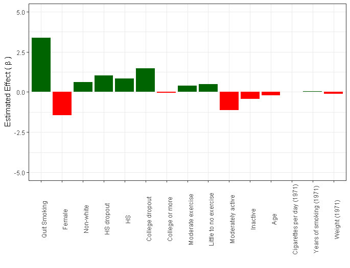
Figure 1: Standardization model coefficients representing the estimated effect. The effect for "Quit Smoking" is the estimate for the causal effect of treatment. All other values represent effect modification and adjustment for confounding bias.

We can visualizes the effect sizes of the treatment and confounding variables; see Figure 1. The model estimates quitting smoking will cause weight loss of approximately 3.38 kilograms. While this model theoretically produces an unbiased estimate of the effect of quitting smoking on weight, there is uncertainty if the model is correctly specified for the problem. For this reason, we will see conflicting estimates among different models. For this reason, we generate an estimate for each model in the package for comparison.

IP Weighting

The ipweighting() function produces a similar output but using the inverse probability methodology instead. It has the following structure:

ipweighting(data, f = NA, family = gaussian(), p.f = NA,  p.simple = pkg.env$simple, p.family = binomial(), p.scores = NA,  SW = TRUE, n.boot = 0, ...)

The parameters are very similar to standardization() except there is no option to override simple since the final model is weighted least squares (WLS) of simply treatment and outcome. The same parameters are available for the underlying propensity model and are given a prefix. For example, to pass a specific formula to the propensity model, the p.f parameter should be used and to change the family of the propensity model, the p.family parameter should be used. This model can also be called separately and has the following structure:

propensity_scores(data, f = NA, simple = pkg.env$simple,  family = binomial(), ...)

The propensity model will fit the data to predict the probability of treatment using the covariates. The IP weighting model will fit a WLS model with the inverse of the propensity scores. By default, standardized weights are used but this can be changed by setting SW to FALSE If the user wants another propensity model not provided in the package, the propensity scores can be manually input into the function via the p.scores parameter. This parameter will override the modeling of the propensity scores and use the ones given by the user.

R> ip.model <- ipweighting(nhefs, p.simple = TRUE)R> print(ip.model)

Call:  glm(formula = wt82_71 ~ qsmk, family = family, data = data,            weights = weights)Coefficients:(Intercept)        qsmk1      2.553        2.569Degrees of Freedom: 1565 Total (i.e. Null);  1564 ResidualNull Deviance:    115000Residual Deviance: 112900 AIC: 11010Average treatment effect of qsmk:Estimate -  2.56858SE       -  0.477962795% CI   - ( 1.63179 ,  3.505369 )

The coefficient of the WLS model is used as the estimate of the average treatment effect. For this reason, n.boot is set to 0, and the standard error calculated by glm() is used instead. If n.boot is set to a positive value, the standard error calculated from the bootstrapping will be used instead. In the example above, p.simple is set to TRUE which means the underlying propensity model will use the autogenerated formula without interactions.

Outcome Regression

The function outcome_regression() builds a linear model using all covariates. The treatment effects are stratified within the levels of the covariates. The model will automatically provide all discrete covariates in a contrast matrix. This is done using the glht() function from the multcomp package; see Hothorn et al. (2008). To view estimated change in treatment effect from continuous variables, a list called contrasts, needs to be given with specific values to estimate. A vector of values can be given for any particular continuous variable. The function has the structure:

outcome_regression(data, f = NA, simple = pkg.env$simple, family = gaussian(),  contrasts = list(), ...)

The parameters are similar to standardization(). Additionally, there is another parameter contrasts which specifies the values of any continuous variables to include in the analysis. This should be a named list corresponding to the continuous variables in the dataset.

R> outreg.mod <- outcome_regression(data = nhefs,+                                   contrasts = list(age = c(21, 30, 40),+                                                smokeintensity = c(5, 20)))R> print(outreg.mod)

Average treatment effect of qsmk:                                         Estimate Std. Error     2.5 %   97.5 %Effect of qsmk at qsmk1                 0.5509460   2.822912 -4.981860 6.083752Effect of qsmk at sex1                 -0.8862384   2.868126 -6.507662 4.735185Effect of qsmk at race1                 1.1377836   2.872922 -4.493039 6.768607Effect of qsmk at education2            1.3684229   2.862462 -4.241899 6.978745Effect of qsmk at education3            1.1333579   2.846699 -4.446070 6.712786Effect of qsmk at education4            2.0750350   2.890966 -3.591154 7.741224Effect of qsmk at education5            0.3717038   2.855788 -5.225537 5.968945Effect of qsmk at exercise1             0.8573187   2.854214 -4.736839 6.451476Effect of qsmk at exercise2             0.9060249   2.869506 -4.718103 6.530153Effect of qsmk at active1              -0.3951223   2.844877 -5.970979 5.180734Effect of qsmk at age of 21             0.8095362   2.240964 -3.582673 5.201746Effect of qsmk at age of 30             0.9203606   2.229701 -3.449772 5.290494Effect of qsmk at age of 40             1.0434988   2.401860 -3.664059 5.751057Effect of qsmk at smokeintensity of 5   0.7749600   2.786389 -4.686262 6.236182Effect of qsmk at smokeintensity of 20  1.4470019   2.745636 -3.934346 6.828349

The above example stratifies by all discrete variables and five specific values of continuous variables. The standard error and confidence interval for each strata are included. A p-value for each strata can also be seen by using summary() on the model.

Propensity Matching

The function propensity_matching() uses either stratification or standardization to model an outcome conditional on the propensity scores. In stratification, the model will break the propensity scores into groups and output a glht() object based off a contrast matrix which estimates the change in average causal effect within groups of propensity scores. This is a form of outcome regression. In standardization, the model will output a standardization() object that conditions on the propensity strata rather than the covariates. The model can also predict the expected outcome. It has the following structure:

propensity_matching(data, f = NA, simple = pkg.env$simple, p.scores = NA,  p.simple = pkg.env$simple, type = "strata", grp.width = 0.1,  quant = TRUE, ...)

The parameters are similar to ipweighting() for both the outcome and propensity elements of the model. Additionally, there is a parameter strata which determines whether the model uses standardization or stratification via outcome regression. To determine how the strata of propensity scores are made, the user can specify to use quantiles with the quant parameter. If it is set to FALSE then grp.width will be used instead to make groups with some width between 0 and 1. It should be noted there may be issues with positivity in the groups with smaller widths. All strata of propensity scores must have a non-zero number of samples in order for the model to work properly. If standardization is used, then the propensity scores are modeled as a continuous value, and unless a specific formula is given, the squared term along with the interaction between propensity scores and treatment are included.

R> pm.model <- propensity_matching(nhefs.nmv, type = "strata")R> print(pm.model)

Average treatment effect of qsmk:                                             Estimate Std. ErrorEffect of qsmk for p.score in [0.051,0.124] 0.2073431   2.394879Effect of qsmk for p.score in (0.124,0.16]  4.9139249   1.728781Effect of qsmk for p.score in (0.16,0.189]  4.6981335   1.598030Effect of qsmk for p.score in (0.189,0.212] 2.2821425   1.454161Effect of qsmk for p.score in (0.212,0.237] 3.8269831   1.441765Effect of qsmk for p.score in (0.237,0.266] 4.9434473   1.351889Effect of qsmk for p.score in (0.266,0.299] 5.5667116   1.404462Effect of qsmk for p.score in (0.299,0.344] 2.3506362   1.312138Effect of qsmk for p.score in (0.344,0.417] 0.9952724   1.278424Effect of qsmk for p.score in (0.417,0.777] 3.1047566   1.222830                                                 2.5 %   97.5 %Effect of qsmk for p.score in [0.051,0.124] -4.4865341 4.901220Effect of qsmk for p.score in (0.124,0.16]   1.5255755 8.302274Effect of qsmk for p.score in (0.16,0.189]   1.5660526 7.830214Effect of qsmk for p.score in (0.189,0.212] -0.5679605 5.132246Effect of qsmk for p.score in (0.212,0.237]  1.0011753 6.652791Effect of qsmk for p.score in (0.237,0.266]  2.2937930 7.593102Effect of qsmk for p.score in (0.266,0.299]  2.8140173 8.319406Effect of qsmk for p.score in (0.299,0.344] -0.2211070 4.922379Effect of qsmk for p.score in (0.344,0.417] -1.5103923 3.500937Effect of qsmk for p.score in (0.417,0.777]  0.7080541 5.501459

The above example uses the stratification option and provides the standard error and confidence interval for each strata. Similar to outcome_regression() a p-value for each strata can also be seen by using summary() on the model.

Doubly-Robust Estimator

The doubly_robust() function trains both an outcome model and a propensity model to generate predictions for the outcome and probability of treatment respectively. By default, the model uses standardization() and propensity_scores() to form a doubly-robust model between standardization and IP weighting. Alternatively, any outcome and propensity models can be provided instead, but must be compatible with the predict generic function in R. Since many propensity models may not predict probabilities without additional arguments into the predict function, the predictions themselves can be given for both the outcome and propensity scores. It has the following structure:

doubly_robust(data, out.mod = NULL, p.mod = NULL, f = NA, family = gaussian(),  simple = pkg.env$simple, scores = NA, p.f = NA, p.simple = pkg.env$simple,  p.family = binomial(), p.scores = NA, n.boot = 50, ...)

It has the parameters for both standardization() and propensity_scores() so the user has full control of the underlying models. Additionally, out.mod and p.mod can be specified to a model trained externally as long as they predict the outcome and probability of treatment respectively. If the generic function predict() cannot be used with either model, the user can also specify the predictions in place of the model using the scores and p.score parameters respectively.

R> p.model <- propensity_scores(nhefs.nmv, simple = T)R> p.scores <- p.model$p.scoresR> out.mod <- propensity_matching(data = nhefs.nmv)R> db.model <- doubly_robust(out.mod = out.mod, p.scores = p.scores, data = nhefs.nmv)R> print(db.model)

Outcome ModelCall:glm(formula = wt82_71 ~ qsmk * p.grp, data = data)Predictions:   Min. 1st Qu.  Median    Mean 3rd Qu.    Max.-0.7685  1.0638  2.8130  2.6383  3.4145  7.9550Propensity ModelCall:NULLPredictions:   Min. 1st Qu.  Median    Mean 3rd Qu.    Max.0.04011 0.18249 0.24077 0.25734 0.32152 0.78131Average treatment effect of qsmk:Estimate -  2.57336SE       -  0.469239695% CI   - ( 1.653667 ,  3.493052 )

In the example above, a random forest model was used to generate the propensity scores; see Liaw and Wiener (2002). Since this model needs a specific parameter in the predict() function and subsetting of the result to obtain propensity scores, the calculations are done externally. The outcome model used is a propensity_matching() model with all default values. Printing the estimator, a summary of the predictions from each model is given, and the estimate for the average treatment effect along with the standard error and confidence interval. Since the propensity scores were the input for the model rather than a propensity model, the call in the output is empty. Like the models in the package, this estimator is also compatable with generic functions summary() and predict() The summary() function will print a summary of both models. If there are not two models such as this example, the output will be empty for that part of the estimator. The predict() function used on the estimator will simply return the estimated average treatment effect.

Standard Instrumental Variable Estimator

The iv_est() function calculates the standard IV estimand using the conditional means on a given instrumental variable. This is currently the only nonparametric function implemented in the package. While there is a method to design this estimator parametrically, that option is not implemented at this time. It has the following structure:

iv_est(IV, data, n.boot = 50)

The instrumental variable can be binary or continuous. A string of the instrumental variable name should be assigned to the IV parameter.

R> nhefs.iv <- nhefs[which(!is.na(nhefs$wt82) & !is.na(nhefs$price82)),]R> nhefs.iv$highprice <- as.factor(ifelse(nhefs.iv$price82>=1.5, 1, 0))R> nhefs.iv$qsmk <- as.factor(nhefs.iv$qsmk)R> iv_est("highprice", nhefs.iv, n.boot = 0)

      ATE SE 2.5 % 97.5 %1 2.39627 NA    NA     NA

In this example, a new variable was created that was an instrumental variable for the data. The parameter n.boot was set to zero to show that bootstrapping would not occur unless the parameter is a positive integer. A data frame is returned with the estimate standard error and confidence interval.

Single parameter G-estimation

The gestimation() function trains either a linear mean model for closed form estimations or a grid search. By default, the function will perform a grid search and require values for the search. It has the following structure:

gestimation(data, grid, ids = list(), f = NA, family = binomial(), simple = pkg.env$simple,  p.f = NA, p.simple = pkg.env$simple, p.family = binomial(), p.scores = NA, SW = TRUE,  n.boot = 100, type = "one.grid", ...)

The formula and propensity parameters have the same meaning as previous functions in relation to an underlying propensity model. In a grid search, a geeglm() model is used for estimation. The ids parameter is to identify the clusters of the geeglm() model and should be the same as the number of samples in the data. The gestimation() function will use the row names by default. Additionally, values for the search grid are required. These can be any list of numeric values that are within the estimated range for the treatment effect. The 95% convidence interval for this method is constructed using the minimum and maximum values for $\beta$ that are statistically significant ($p<0.05$). In a linear mean model, a closed form g-estimation will be performed and the confidence interval will be constructed by bootstrapping with the n.boot parameter.

    R> gest.model <- gestimation(nhefs.nmv, type = "one.linear")    R> print(gest.model)

    Call:  glm(formula = f, family = family, data = data, weights = weights)Coefficients:                       (Intercept)                                sex1                        -2.3321457                          -0.6143474                             race1                          education2                        -0.7963585                           0.0973526                        education3                          education4                         0.1996545                           0.2953593                        education5                           exercise1                         0.6016503                           0.4167123                         exercise2                             active1                         0.3579257                           0.1113038                           active2                                 age                         0.1361076                           0.1408696                      I(age * age)                      smokeintensity                        -0.0009840                          -0.0718707I(smokeintensity * smokeintensity)                            smokeyrs                         0.0008645                          -0.0847584            I(smokeyrs * smokeyrs)                                wt71                         0.0009799                          -0.0243495                    I(wt71 * wt71)                         0.0001830Degrees of Freedom: 1565 Total (i.e. Null);  1547 ResidualNull Deviance:    1981Residual Deviance: 1853 AIC: 1968Average treatment effect of qsmk:Estimate -  3.467472SE       -  0.552054295% CI   - ( 2.385465 ,  4.549478 )

Results

After generating an estimate from each model in the package, we compare each model estimate including its 95% confidence interval; see Figure 2. Since doubly-robust models only require one of the two models to be correctly specified, we use this as our baseline comparison among all the estimators.

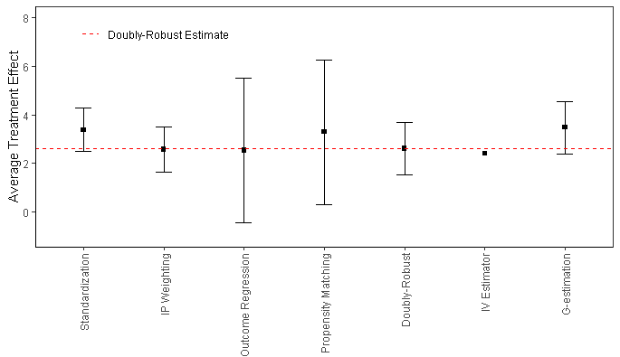
Figure 2: ATE estimates from each estimator in the CausalModels package. The error bars for each point estimate represent the 95% Wald confidence interval from the estimator.

IP weighting, outcome regression and the instrumental variable estimator are all in agreement with the double-robust model that the causal effect of quitting smoking on weight is approximately a weight loss of 2.4 kilograms. For this reason, we can claim all of these models are correctly specified and give an unbiased estimate of the causal effect. We can also infer standardization, propensity matching, and g-estimation seem to be wrongly specified estimating approximately 3.5 kilograms for this problem, and we should not assume this accurately estimates the true causal effect.

Conclusion

Research in causal inference requires strict attention to possible biases and correct model specification. CausalModels offers a single source for an array of structural models for causal inference established in Hernán and Robins (2020) with a simple modeling pipeline for easy model comparison. The package focuses on abstracting repetitive steps in causal analysis while encouraging the user to adjust for bias with correct model specification. This is done while also allowing the user to adjust any model to the same extent as they would using base R. We look forward to growing the package to support more methods and a wider array of variables in the future.

Availability

This paper presented introductory concepts to causal inference and fundamental modeling methods included in the CausalModels package available from the Comprehensive R Archive Network (CRAN) at https://CRAN.R-project.org/package=CausalModels.

Joshua Wolff Anderson
Department of Intelligent Systems
University of Pittsburgh
Pittsburgh PA, USA
jwa45@pitt.edu

Cyril Rakovski
Department of Mathematics
Chapman University
Orange CA, USA
rakovski@chapman.edu

References

- Angrist et al. (1996) J. D. Angrist, G. W. Imbens, and D. B. Rubin. Identification of causal effects using instrumental variables. Journal of the American statistical Association, 91(434):444–455, 1996.
- Arnold et al. (2016) B. F. Arnold, A. Ercumen, J. Benjamin-Chung, and J. M. Colford Jr. Brief report: negative controls to detect selection bias and measurement bias in epidemiologic studies. Epidemiology (Cambridge, Mass.), 27(5):637, 2016.
- Benkeser (2017) D. Benkeser. drtmle: Doubly-robust nonparametric estimation and inference. R package version, 1(0), 2017.
- Blakely et al. (2020) T. Blakely, J. Lynch, K. Simons, R. Bentley, and S. Rose. Reflection on modern methods: when worlds collide—prediction, machine learning and causal inference. International journal of epidemiology, 49(6):2058–2064, 2020.
- Bodory and Huber (2018) H. Bodory and M. Huber. The causalweight package for causal inference in r. Technical report, Université de Fribourg, 2018.
- Caliendo and Kopeinig (2008) M. Caliendo and S. Kopeinig. Some practical guidance for the implementation of propensity score matching. Journal of economic surveys, 22(1):31–72, 2008.
- Fang et al. (2012) G. Fang, J. M. Brooks, and E. A. Chrischilles. Apples and oranges? interpretations of risk adjustment and instrumental variable estimates of intended treatment effects using observational data. American journal of epidemiology, 175(1):60–65, 2012.
- Funk et al. (2011) M. J. Funk, D. Westreich, C. Wiesen, T. Stürmer, M. A. Brookhart, and M. Davidian. Doubly robust estimation of causal effects. American journal of epidemiology, 173(7):761–767, 2011.
- Greifer (2020) N. Greifer. A guide to using weightit for estimating balancing weights, 2020.
- Hammerton and Munafò (2021) G. Hammerton and M. R. Munafò. Causal inference with observational data: the need for triangulation of evidence. Psychological Medicine, 51(4):563–578, 2021.
- Hennessy et al. (2016) J. Hennessy, T. Dasgupta, L. Miratrix, C. Pattanayak, and P. Sarkar. A conditional randomization test to account for covariate imbalance in randomized experiments. Journal of Causal Inference, 4(1):61–80, 2016.
- Hernán and Robins (2006) M. A. Hernán and J. M. Robins. Estimating causal effects from epidemiological data. Journal of Epidemiology & Community Health, 60(7):578–586, 2006.
- Hernán and Robins (2020) M. A. Hernán and J. M. Robins. Causal Inference: What If. Boca Raton: Chapman & Hall/CRC, 2020.
- Hernán et al. (2004) M. A. Hernán, S. Hernández-Díaz, and J. M. Robins. A structural approach to selection bias. Epidemiology, pages 615–625, 2004.
- Hothorn et al. (2008) T. Hothorn, F. Bretz, and P. Westfall. Simultaneous inference in general parametric models, 2008.
- Huntington-Klein and Barrett (2021) N. Huntington-Klein and M. Barrett. causaldata: Example Data Sets for Causal Inference Textbooks, 2021. URL https://CRAN.R-project.org/package=causaldata. R package version 0.1.3.
- Judea (2010) P. Judea. An introduction to causal inference. The International Journal of Biostatistics, 6(2):1–62, 2010.
- Liaw and Wiener (2002) A. Liaw and M. Wiener. Classification and regression by randomforest. R News, 2(3):18–22, 2002. URL https://CRAN.R-project.org/doc/Rnews/.
- R Core Team (2021) R Core Team. R: A Language and Environment for Statistical Computing. R Foundation for Statistical Computing, Vienna, Austria, 2021. URL https://www.R-project.org/.
- Rehkopf et al. (2016) D. H. Rehkopf, M. M. Glymour, and T. L. Osypuk. The consistency assumption for causal inference in social epidemiology: when a rose is not a rose. Current epidemiology reports, 3(1):63–71, 2016.
- Robins et al. (2000) J. M. Robins, M. A. Hernan, and B. Brumback. Marginal structural models and causal inference in epidemiology, 2000.
- Rosenbaum (2005) P. R. Rosenbaum. Observational study. Encyclopedia of statistics in behavioral science, 2005.
- Rubin and Thomas (1996) D. B. Rubin and N. Thomas. Matching using estimated propensity scores: relating theory to practice. Biometrics, pages 249–264, 1996.
- Shaughnessy et al. (2000) J. J. Shaughnessy, E. B. Zechmeister, and J. S. Zechmeister. Research methods in psychology. McGraw-Hill, 2000.
- Sjölander and Hössjer (2021) A. Sjölander and O. Hössjer. Novel bounds for causal effects based on sensitivity parameters on the risk difference scale. Journal of Causal Inference, 9(1):190–210, 2021.
- Tikka and Karvanen (2018) S. Tikka and J. Karvanen. Identifying causal effects with the r package causaleffect. arXiv preprint arXiv:1806.07161, 2018.
- Van Stralen et al. (2010) K. Van Stralen, F. Dekker, C. Zoccali, and K. Jager. Confounding. Nephron Clinical Practice, 116(2):c143–c147, 2010.
- VanderWeele (2015) T. VanderWeele. Explanation in causal inference: methods for mediation and interaction. Oxford University Press, 2015.
- Wallace et al. (2017) M. P. Wallace, E. E. Moodie, and D. A. Stephens. An r package for g-estimation of structural nested mean models. Epidemiology, 28(2):e18–e20, 2017.
- Westreich and Cole (2010) D. Westreich and S. R. Cole. Invited commentary: positivity in practice. American journal of epidemiology, 171(6):674–677, 2010.