An extended latent factor framework for
ill-posed linear regression

Abstract

The classical latent factor model for linear regression is extended by assuming that, up to an unknown orthogonal transformation, the features consist of subsets that are relevant and irrelevant for the response. Furthermore, a joint low-dimensionality is imposed only on the relevant features vector and the response variable. This framework allows for a comprehensive study of the partial-least-squares (PLS) algorithm under random design. In particular, a novel perturbation bound for PLS solutions is proven and the high-probability $L^{2}$-estimation rate for the PLS estimator is obtained. This novel framework also sheds light on the performance of other regularisation methods for ill-posed linear regression that exploit sparsity or unsupervised projection. The theoretical findings are confirmed by numerical studies on both real and simulated data.

Keywords:

Ill-posed regression; dimensionality reduction; latent factor models; partial least squares.

MSC: Primary: 62H25, 65F22; Secondary: 65F10, 62J05.

1 Introduction

Given some data set $(\mathbf{X},\mathbf{y})\in\mathbb{R}^{n\times p}\times\mathbb{R}^{n}$ consisting of $n\geq 1$ i.i.d. realizations $(\mathbf{x}_{i},y_{i})$ of the the same population random pair $(\mathbf{x},y)\in\mathbb{R}^{p}\times\mathbb{R}$, we consider the problem of learning an ill-posed linear model, in the least-squares sense. Such models arise in many high-dimensional data sets in biology, genomics, neuroscience and finance and are the symptom of a possibly low-dimensional generating process. We propose a novel framework for ill-posed regression that will be useful to practitioners working in applications with strict interpretability requirements.

1.1 Ill-posedness and interpretability

The $L^{2}$-minimum-norm least-squares estimator computed from the sample is $\widehat{\bm{\beta}}_{ls}:=\widehat{\bm{\Sigma}}_{\mathbf{x}}^{+}\widehat{\bm{\Sigma}}_{\mathbf{x},y}$, this is the product between the Moore-Penrose inverse of the sample covariance matrix $\widehat{\bm{\Sigma}}_{\mathbf{x}}:=n^{-1}\mathbf{X}^{\top}\mathbf{X}$ and the sample covariance vector $\widehat{\bm{\Sigma}}_{\mathbf{x},y}:=n^{-1}\mathbf{X}^{\top}\mathbf{y}$. Due to the ill-posedness of the sample covariance matrix, any prediction of the response in terms of the sample least-squares might be statistically misleading. Kim (2019) shows that multicollinearity can be measured in terms of the condition number $\widetilde{\kappa}$ (the ratio between the largest and smallest eigenvalue) of the sample covariance matrix relative to the standardised data set $\widetilde{\mathbf{X}}$ obtained by centering/scaling $\mathbf{X}$ columnwise. The author argues that multicollinearity becomes detrimental as soon as $\widetilde{\kappa}^{1/2}>30$, which is roughly $\log_{10}(\widetilde{\kappa})>3$, and one should follow some principled regularization strategy to overcome the issue. To put this into perspective, data sets involving molecular-dynamics simulations, a technique first devised by McCammon et al. (1977), are notoriously ill-posed with condition numbers way above $10^{4}$, thus one can expect $\log_{10}(\widetilde{\kappa})>4$ despite the large sample size ($n\gg p$) of such applications. The situation is even more dramatic for genomics data sets where one observes a large number of genes but a limited amount of information ($p\gg n$), essentially resulting in perfect collinear features and infinite condition number. In general, one expects the quality of inference to be affected only by the correlation between the features that are actually relevant for the response.

1.2 Regularization of ill-posed linear models

When interpretability is paramount, dimensionality reduction is crucial to avoid misleading statistical results. Most regularization strategies exploit, in some way or another, either penalization or projection.

1.2.1 Penalization

Penalization-based methods such as Tikhonov/Ridge regression, see Tikhonov (1943) or Hoerl (1962), compute estimators of the form $\widehat{\bm{\beta}}_{2,\lambda}:=(\widehat{\bm{\Sigma}}_{\mathbf{x}}+\lambda\mathbf{I}_{p})^{-1}\widehat{\bm{\Sigma}}_{\mathbf{x},y}$ with possibly small penalization parameter $\lambda>0$. A small penalization parameter guarantees a small bias, but does not induce dimensionality reduction and the condition number of the perturbed matrix is still large. The same can be said for $L^{q}$-penalization methods with $q>1$.

The LASSO, devised by Tibshirani (1996), is a special penalization-based method that performs dimensionality reduction by enforcing sparsity. This method selects a regular subset $\mathbf{X}_{\lambda}$ of the features, depending on some penalization parameter $\lambda>0$, and yields the corresponding least-squares estimator $\widehat{\bm{\beta}}_{1,\lambda}:=\widehat{\bm{\Sigma}}_{\mathbf{x}_{\lambda}}^{-1}(\widehat{\bm{\Sigma}}_{\mathbf{x}_{\lambda},y}-\lambda\bm{\xi})$, where $\bm{\xi}$ is a vector of equicorrelation signs, see Section 2 by Tibshirani (2013) for details. The LASSO estimator is ill-posed unless the condition number of the reduced covariance matrix is small, a classical assumption for this to happen is the restricted eigenvalue condition by Bickel et al. (2009) or one of the many variants discussed by van de Geer and Bühlmann (2009).

1.2.2 Projection

Projection-based methods achieve dimensionality reduction by projecting the features onto chosen linear subspaces and by computing the sample least-squares on the projected data set $\widehat{\bm{\beta}}_{\mathbf{P}_{s}}:=\mathbf{P}_{s}(\mathbf{P}_{s}^{\top}\widehat{\bm{\Sigma}}_{\mathbf{x}}\mathbf{P}_{s})^{-1}\mathbf{P}_{s}^{\top}\widehat{\bm{\Sigma}}_{\mathbf{x},y}$, where $1\leq s\leq p$, $\mathbf{P}_{s}\in\mathbb{R}^{p\times s}$ and $\mathbf{P}_{s}^{\top}\mathbf{P}_{s}=\mathbf{I}_{s}$. Principal-components-regression (PCR), first devised by Hotelling (1933), projects onto $\mathcal{R}(\mathbf{P}_{s}\mathbf{P}_{s}^{\top})=\operatorname{span}\{\widehat{\mathbf{v}}_{1},\ldots,\widehat{\mathbf{v}}_{s}\}$ where $\widehat{\mathbf{v}}_{i}$’s are the top $s$ eigenvectors of $\widehat{\bm{\Sigma}}_{\mathbf{x}}$. Under a latent factor regression setting, Bing et al. (2021) obtain finite-sample risk bounds for unsupervised estimators $\widehat{\bm{\beta}}_{\widehat{\mathbf{P}}}$ whose projection $\widehat{\mathbf{P}}$ only depends on the design matrix $\mathbf{X}$, but not on the response vector $\mathbf{y}$. They propose an adaptive PCR estimator $\widehat{\bm{\beta}}_{pcr,\widehat{s}}$ and show that the true number of latent factors is consistently estimated.

Partial-least-squares (PLS), as proposed by Helland (1990), projects the data onto the $s$-dimensional Krylov space $\mathcal{R}(\mathbf{P}_{s}\mathbf{P}_{s}^{\top})=\operatorname{span}\{\widehat{\bm{\Sigma}}_{\mathbf{x},y},\widehat{\bm{\Sigma}}_{\mathbf{x}}\widehat{\bm{\Sigma}}_{\mathbf{x},y}\ldots,\widehat{\bm{\Sigma}}_{\mathbf{x}}^{s-1}\widehat{\bm{\Sigma}}_{\mathbf{x},y}\}$ computed from both the sample covariance matrix and vector. Under a latent factor regression setting, Singer et al. (2016) recover high-probability estimation rates for the sample PLS. They propose an adaptive PLS estimator $\widehat{\bm{\beta}}_{pls,\widehat{s}}$ but the choice of latent dimension hinges on a heuristic stopping rule that might overestimate the true number of latent factors.

1.3 A novel framework for ill-posed regression

We argue that many interesting applications fall outside the scope of the available literature on latent factor models or sparse models. In fact, the main underlying feature of the latent factor models introduced by Stock and Watson (2002) and Bai and Ng (2002), and later studied by Singer et al. (2016) for PLS and Bing et al. (2021) for PCR, is that the true number of latent factors can be consistently estimated in terms of the eigenvalues of the sample covariance matrix. That is to say, all the main principal components are relevant for the response. The sentiment that this is a restrictive assumption is quite old, Cox (1968), see Section 3 (ii) (c), and other authors suggest that there is no logical reason for the principal components to contain any information at all on the response. Any unsupervised strategy for dimensionality reduction that only uses the information of $\mathbf{X}$, while being agnostic to the response vector $\mathbf{y}$, will lead to interpretability loss in ill-posed problems. The same argument applies to the sparsity assumption, which essentially requires that only a few columns of the features $\mathbf{X}$ are actually relevant for the response vector $\mathbf{y}$. The concept of sparsity depends on the particular coordinate system of the features and is not robust to rotations of the data. In general, the LASSO might overestimate the number latent factors in all those applications where the model is sparse up to some rotation of the observed data, that is to say, where only a few linear combinations of features (but not the features themselves) are relevant for the response.

Motivated by the above discussion, we propose a novel class of models for the population pair $(\mathbf{x},y)\in\mathbb{R}^{p}\times\mathbb{R}$ that is flexible enough to accommodate the following.

1. Arbitrary subspaces of features that are relevant and irrelevant for the response. We formalize this by assuming the existence of some linear subspace $\mathcal{B}_{y}\subseteq\mathbb{R}^{p}$ of dimension $1\leq d\leq p$, with $\mathbf{x}_{y}\in\mathcal{B}_{y}$ the the relevant features and $\mathbf{x}_{y^{\bot}}:=\mathbf{x}-\mathbf{x}_{y}\in\mathcal{B}_{y}^{\bot}$ the irrelevant features, so that the irrelevant features $\mathbf{x}_{y^{\bot}}$ are uncorrelated from both the response $y$ and the relevant features $\mathbf{x}_{y}$.

2. A joint low-dimensionality of the relevant pair $(\mathbf{x}_{y},y)$ in terms of some random vector of latent features $\mathbf{q}\in\mathbb{R}^{m}$ with $1\leq m\leq d$.

When the relevant features $\mathbf{x}_{y}$ in (i) are a subset of the original features $\mathbf{x}$, the model is $d$-sparse. Otherwise, it is sparse up to an orthogonal transformation. When all the features in (i) are assumed to be relevant, that is $\mathbf{x}=\mathbf{x}_{y}$, our model in (ii) essentially reduces to the standard latent factor regression setting studied, among others, by Singer et al. (2016) for PLS and by Bing et al. (2021) for PCR. Although formally similar to the recent effort by Fan et al. (2023) to bridge the gap between latent and sparse models, our proposed framework is more flexible. In fact, Fan et al. (2023) discuss in their Remark 2 that their regularity assumptions essentially guarantee that the true number of factors can be consistently estimated by the eigenvalue ratio method by Lam and Yao (2012) and Ahn and Horenstein (2013). This is equivalent to assuming that there are no irrelevant features, that is $\mathbf{x}=\mathbf{x}_{y}$ in our condition (i) above.

To fix the ideas, consider a toy model with $p=3$, so that the features live on the three-dimensional space; $d=2$, so that only a two-dimensional projection of the features is correlated with the response; $m=1$, so that the response is a function of some one-dimensional projection of the features. In this setting, one can identify three orthogonal directions: i) the direction of variation of the latent factor; ii) the direction orthogonal to the latent factor but inside the relevant plane; iii) the direction of variation of the irrelevant feature. Figure 1 shows a realization of such a toy model where one observes i.i.d. realizations of some rotation of $\mathbf{x}=(x_{1},x_{2},x_{3})$ with $x_{1},x_{2},x_{3}$ real and independent random variables $x_{1}\in\mathcal{N}(0,1)$, $x_{2}\sim\mathcal{N}(0,0.5)$ and $x_{3}\sim\mathcal{U}(-4,4)$. The response $y$ only depends on the one-dimensional factor generated by $(x_{1},0,0)$. The orthogonal residual generated by $(0,x_{2},0)$ adds a small noise to the latent factor and yields the two-dimensional plane of relevant features $(x_{1},x_{2},0)$. The remaining irrelevant feature generated by $(0,0,x_{3})$ can have a large variance and become the main direction of variation of the features, despite being uncorrelated with the response. The model is sparse if the axis of main variations are aligned with the columns of the design matrix.

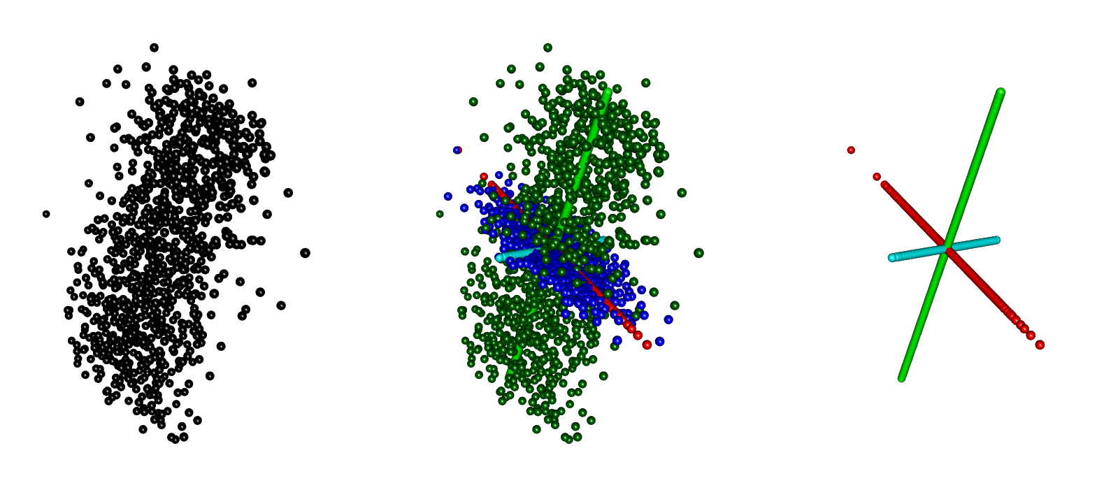
Figure 1: A data set consistent with our novel framework with $p=3,\ d=2,\ m=1$. A sample of $n=1000$ observations (black) in the three-dimensional space; the one-dimensional factor (red); the orthogonal residual (cyan) and the two-dimensional plane (blue) of relevant features; the irrelevant feature (green) uncorrelated with the response.

1.4 Novel insights on partial least squares

Despite the theory of LASSO and PCR being well established and extensively studied, our proposed framework provides new insights on the performance of regularization methods relying on sparsity or unsupervised projection. Furthermore, it allows for a comprehensive study of the PLS algorithm for ill-posed linear regression under random design. We summarize our contributions below.

1.4.1 Applications of partial least squares

Our results are consistent with the heuristic findings of Krivobokova et al. (2012), which we revisit here. We consider data generated by the molecular dynamics simulations for the yeast aquaporin (Aqy1), the gated water channel of the yeast Pichia pastoris. The data are given as Euclidean coordinates of $783$ atoms, thus $p=783\times 3=2.349$ features, of Aqy1 observed in a 100 nanosecond time frame, split into $n=20.000$ equidistant observations. Additionally, the diameter of the channel $y_{t}$ at time $t$ is given, measured by the distance between two centers of mass of certain residues of the protein. The aim of the analysis is to identify the collective motions of the atoms responsible for the channel opening. Such setup is compatible with our proposed framework, since it is conceivable that only atoms that are in the vicinity of the water channel will be relevant for the response. Also, it seems unlikely that the atoms that are closer to the water channel also correspond to the principal components of the sample covariance matrix. An educated guess would be that PLS requires much less latent components than PCR in order to explain the same amount of information, and this is exactly what Krivobokova et al. (2012) show in their Figure 3. Similarly, despite only a small number of atoms being relevant, the local correlation between particles might be strong, especially among atoms belonging to the same amino-acid chain. Thus, we expect LASSO to be ill-posed in such setups. To investigate such hypothesis, we repeat the experiment by Krivobokova et al. (2012) and include a comparison between LASSO, PCR and PLS. We refer the reader to Section 3 for a detailed discussion, Figure 4 confirms that PLS outperforms PCR in terms of explained correlation and prediction, and LASSO in terms of prediction and conditioning.

Wang et al. (2011) compare estimates from variations of the LASSO method on a glioblastoma microarray data set consisting of $n=120$ clinical samples for $p=3.600$ genes and show that their proposed random-LASSO method outperforms the other variations. Despite the popularity of the PLS method for genomic data sets, as discussed by Boulesteix and Strimmer (2006), Chun and Keleş (2010) show that PLS estimates can be inconsistent as soon as the ratio $p/n$ does not vanish in the limit of increasing sample size. To overcome this issue, they propose a sparse-PLS method and provide numerical guarantees. Under our novel framework, we show that PLS estimates can be consistent even when $p/n$ does not vanish, thus confirming its desirability for genomics applications.

1.4.2 Theory of partial least squares

Singer et al. (2016) show that the PLS algorithm is equivalent to the conjugate-gradient-normal-equation (CGNE) algorithm for which Nemirovskii (1986) obtained perturbation bounds. The same technical ideas are found in the seminal work by Blanchard and Krämer (2016) who provide convergence rates for kernel-CGNE for nonparametric regression in Hilbert spaces. The classical theory for CGNE presented by Hanke (1995) is very general and only guarantees perturbation bounds when the number of latent components is selected according to some ad-hoc stopping rule. Many simplifications arise when one deals with finite-dimensional linear models and, for such problems, the CGNE algorithm can actually be traced back to Hestenes and Stiefel (1952).

We develop novel proof techniques to derive the properties of the PLS method both in population and in sample. Under our novel framework, our parameters of interest are the oracle vector $\bm{\beta}_{0}:=\mathbf{P}\bm{\alpha}_{0}\in\mathbb{R}^{p}$, where $\bm{\alpha}_{0}\in\mathbb{R}^{m}$ is the true latent vector of coefficients, and the oracle $m$-dimensional linear subspace $\mathcal{B}_{0}:=\mathcal{R}(\mathbf{P}\mathbf{P}^{\top})\subseteq\mathbb{R}^{p}$. We exploit a seminal work by Carpraux et al. (1994) and Kuznetsov (1997) on the stability of Krylov spaces to deduce a general perturbation result for PLS solutions that is of independent interest, see our Theorem A.15 in Appendix A.3. This essentially extends to PLS solutions the classical perturbation bounds for least-squares solutions derived by Wei (1989), see Theorem A.9 in Appendix A.3. In particular, we can now compare PLS solutions that use the same number of latent components, without invoking heuristic stopping rules. From this, we deduce two main results. First, we show in Theorem 2.7 that, if the noise level $\sigma_{0}^{2}$ is well-separated from the minimum eigenvalue of the covariance matrix $\bm{\Sigma}_{\mathbf{q}}$ of the latent features, the approximation error of the population PLS $\bm{\beta}_{pls,m}$ relative to the oracle $\bm{\beta}_{0}$ is proportional to $\sigma_{0}^{-2}$ and the condition number of the oracle Krylov space. Second, we provide in Theorem 2.11, under regularity assumptions on the features, high-probability estimation rates of the sample PLS $\widehat{\bm{\beta}}_{pls,m}$ with parameter equal to the true number of factors. When $p>n$, the rate of the sample PLS is driven by the rank of the covariance matrix of the features. When this rank is sufficiently small, the PLS estimates are still well-posed. A similar phenomenon has been observed by Bunea et al. (2022) in the setting of high-dimensional factor regression.

1.5 Notation

We denote vectors in lower-case bold letters $\mathbf{v}\in\mathbb{R}^{p}$ and matrices in upper-case bold letters $\mathbf{V}\in\mathbb{R}^{p\times p}$. We denote $\mathbf{0}_{p}\in\mathbb{R}^{p}$ the vector of zeros and $\mathbf{I}_{p}\in\mathbb{R}^{p\times p}$ the identity matrix. For any integers $1\leq d\leq p$, we denote $\mathbf{I}_{d,p}\in\mathbb{R}^{p\times p}$ the matrix obtained by setting to zero the diagonal entries of $\mathbf{I}_{p}$ in positions $i=d+1,\ldots,p$. We denote $\mathbf{A}^{+}$ the unique generalized inverse of a matrix $\mathbf{A}$, with the convention that $\mathbf{A}^{+}=\mathbf{A}^{-1}$ when the matrix is invertible. For any square matrix $\mathbf{A}\in\mathbb{R}^{d\times d}$, we denote $p_{\mathbf{A}}$ its minimal polynomial. For any symmetric and positive semi-definite matrix $\mathbf{A}$, we denote its condition number as $\kappa_{2}(\mathbf{A}):=\|\mathbf{A}\|_{op}\|\mathbf{A}^{+}\|_{op}$, where $\|\cdot\|_{op}$ is the operator norm for matrices. For any two random vectors $\mathbf{z}_{1},\mathbf{z}_{2}$ for which the outer product $\mathbf{z}_{1}\mathbf{z}_{2}^{\top}$ is well-defined, we denote $\bm{\Sigma}_{\mathbf{z}_{1},\mathbf{z}_{2}}:=\mathbb{E}[\mathbf{z}_{1}\mathbf{z}_{2}^{\top}]$ and $\bm{\Sigma}_{\mathbf{z}_{1}}:=\bm{\Sigma}_{\mathbf{z}_{1},\mathbf{z}_{1}}$. For any two random matrices $\mathbf{Z}_{1},\mathbf{Z}_{2}$ having $n\geq 1$ rows consisting of an arbitrary sample from random vectors $\mathbf{z}_{1},\mathbf{z}_{2}$, we denote $\widehat{\bm{\Sigma}}_{\mathbf{z}_{1},\mathbf{z}_{2}}:=n^{-1}\mathbf{Z}_{1}^{\top}\mathbf{Z}_{2}$ and $\widehat{\bm{\Sigma}}_{\mathbf{z}_{1}}:=\widehat{\bm{\Sigma}}_{\mathbf{z}_{1},\mathbf{z}_{1}}$. For any centered random vector $\mathbf{z}$ with finite second moment, we denote $\widetilde{\mathbf{z}}=\bm{\Sigma}_{\mathbf{z}}^{-1/2}\mathbf{z}$ its isotropic counterpart. For any integer $d\geq 1$, we denote $\mathbb{B}_{2}^{d}(1):=\{\mathbf{v}\in\mathbb{R}^{d}:\|\mathbf{v}\|_{2}\leq 1\}$ the Euclidean closed unit-ball in $\mathbb{R}^{d}$ and $\partial\mathbb{B}_{2}^{d}(1):=\{\mathbf{v}\in\mathbb{R}^{d}:\|\mathbf{v}\|_{2}=1\}$ the corresponding unit-sphere.

1.6 Structure of the paper

The mathematical framework of our model and our main results are given in Section 2. Numerical studies for both simulated and real data are provided in Section 3. An extension to generalized linear models is described in Section 4. All the auxiliary results are given in Appendix A, together with their proof when necessary. The proofs relative to the main sections are in Appendix B.

2 Ill-posed linear models and partial least squares

We introduce some auxiliary notation. For any symmetric and positive-semidefinite matrix $\mathbf{A}\in\mathbb{R}^{d\times d}$, any vector $\mathbf{b}\in\mathbb{R}^{d}$ and any linear subspace $\mathcal{C}\subseteq\mathbb{R}^{d}$, we denote $\operatorname{LS}(\mathbf{A},\mathbf{b},\mathcal{C}):=\mathop{\rm arg\min}_{\bm{\zeta}\in\mathcal{C}}\|\mathbf{A}\bm{\zeta}-\mathbf{b}\|_{2}^{2}$, that is, the set of least-squares solutions to the problem $\mathbf{A}\bm{\zeta}=\mathbf{b}$ over all $\bm{\zeta}\in\mathcal{C}$. It is a classical result, see Corollary 1 by Penrose (1955), that $\operatorname{LS}(\mathbf{A},\mathbf{b},\mathbb{R}^{d})=\{\mathbf{A}^{+}\mathbf{b}+(\mathbf{I}_{d}-\mathbf{A}^{+}\mathbf{A})\bm{\zeta}:\bm{\zeta}\in\mathbb{R}^{d}\}$ and the $L^{2}$-minimum-norm solution $\bm{\zeta}_{ls}:=\mathbf{A}^{+}\mathbf{b}$ belongs to the range $\mathcal{R}(\mathbf{A}^{+})=\mathcal{R}(\mathbf{A})$, see Theorem 20.5.1 by Harville (1997). This means that restricting the least-squares problem to the range of its linear operator always admits unique solution, that is, $\operatorname{LS}(\mathbf{A},\mathbf{b}):=\operatorname{LS}(\mathbf{A},\mathbf{b},\mathcal{R}(\mathbf{A}))=\{\mathbf{A}^{+}\mathbf{b}\}$. Furthermore, one can always replace the vector $\mathbf{b}$ with its projection onto the range $\mathcal{R}(\mathbf{A})$, in fact, $\operatorname{LS}(\mathbf{A},\mathbf{A}\mathbf{A}^{+}\mathbf{b},\mathcal{R}(\mathbf{A}))=\{\mathbf{A}^{+}\mathbf{b}\}$ and $\mathbf{A}\mathbf{A}^{+}\mathbf{b}=\mathbf{b}$ if and only if $\mathbf{b}\in\mathcal{R}(\mathbf{A})$. For any symmetric and positive-semidefinite matrix $\mathbf{A}\in\mathbb{R}^{d\times d}$ and any vector $\mathbf{b}\in\mathcal{R}(\mathbf{A})$, we denote the PLS solutions as $\operatorname{PLS}(\mathbf{A},\mathbf{b}):=\operatorname{LS}(\mathbf{A},\mathbf{b},\mathcal{K}(\mathbf{A},\mathbf{b}))$, where $\mathcal{K}(\mathbf{A},\mathbf{b}):=\operatorname{span}\{\mathbf{b},\mathbf{A}\mathbf{b},\ldots,\mathbf{A}^{d-1}\mathbf{b}\}$ is a Krylov space. Lemma A.6 guarantees that the PLS solution is unique and coincides with the least-squares solution $\operatorname{PLS}(\mathbf{A},\mathbf{b})=\operatorname{LS}(\mathbf{A},\mathbf{b})$. For any $1\leq s\leq d$, we denote $\operatorname{PLS}(\mathbf{A},\mathbf{b},s):=\operatorname{LS}(\mathbf{A},\mathbf{b},\mathcal{K}_{s}(\mathbf{A},\mathbf{b}))$ where $\mathcal{K}_{s}(\mathbf{A},\mathbf{b})$ is the span of the first $s$ vectors of the Krylov basis.

2.1 Population model

We are interested in the least-squares problem of minimizing the risk functional

$$\bm{\beta}\mapsto\ell_{\mathbf{x},y}(\bm{\beta}):=\mathbb{E}\left[(y-\mathbf{x}^{\top}\bm{\beta})^{2}\right]\in\mathbb{R}$$

over all $\bm{\beta}\in\mathbb{R}^{p}$. The gradient of the risk functional is

$$\bm{\beta}\mapsto\nabla_{\bm{\beta}}\ell_{\mathbf{x},y}(\bm{\beta}):=2\mathbb{E}\left[\mathbf{x}\mathbf{x}^{\top}\bm{\beta}\right]-2\mathbb{E}\left[\mathbf{x}y\right]\in\mathbb{R}^{p},$$

and its Hessian

$$\bm{\beta}\mapsto\nabla_{\bm{\beta}}\nabla_{\bm{\beta}}^{\top}\ell_{\mathbf{x},y}(\bm{\beta}):=2\mathbb{E}\left[\mathbf{x}\mathbf{x}^{\top}\right]\in\mathbb{R}^{p\times p}$$

is a positive semi-definite matrix, so the risk functional $\bm{\beta}\mapsto\ell_{\mathbf{x},y}(\bm{\beta})$ is convex everywhere, although possibly not strictly convex. Any element of the set $\{\bm{\beta}\in\mathbb{R}^{p}:\nabla_{\bm{\beta}}\ell_{\mathbf{x},y}(\bm{\beta})=\mathbf{0}_{p}\}$ of critical points of the risk functional satisfies the population normal equation $\bm{\Sigma}_{\mathbf{x}}\bm{\beta}=\bm{\Sigma}_{\mathbf{x},y}$, which admits at least one solution (the set of critical points is non-empty) since Lemma A.1 shows that the covariance vector $\bm{\Sigma}_{\mathbf{x},y}$ always belongs to the range of the covariance matrix $\bm{\Sigma}_{\mathbf{x}}$. With our notation on least-squares problems, the set of critical points can be rewritten as $\operatorname{LS}(\bm{\Sigma}_{\mathbf{x}},\bm{\Sigma}_{\mathbf{x},y},\mathbb{R}^{p})$ and the $L^{2}$-minimum-norm least-squares solution $\bm{\beta}_{ls}:=\bm{\Sigma}_{\mathbf{x}}^{+}\bm{\Sigma}_{\mathbf{x},y}$ is the unique vector in $\operatorname{LS}(\bm{\Sigma}_{\mathbf{x}},\bm{\Sigma}_{\mathbf{x},y}):=\operatorname{LS}(\bm{\Sigma}_{\mathbf{x}},\bm{\Sigma}_{\mathbf{x},y},\mathcal{R}(\bm{\Sigma}_{\mathbf{x}}))$, which is the set of critical points belonging to the range of the covariance matrix $\bm{\Sigma}_{\mathbf{x}}$. This is well-defined even when the conditional distribution of $y|\mathbf{x}$ depends non-linearly on the features.

In what follows, we assume that only a linear projection of the features vector $\mathbf{x}$ is relevant in determining the distribution of $y|\mathbf{x}$.

Assumption 2.1 (Relevant model).

The population random pair $(\mathbf{x},y)\in\mathbb{R}^{p}\times\mathbb{R}$ satisfies the following. For some integer $1\leq d\leq p$ and some matrix $\mathbf{P}_{y}\in\mathbb{R}^{p\times d}$ with $\mathbf{P}_{y}^{\top}\mathbf{P}_{y}=\mathbf{I}_{d}$, let $\mathbf{x}_{y}:=\mathbf{P}_{y}\mathbf{P}_{y}^{\top}\mathbf{x}\in\mathbb{R}^{p}$ be the vector of relevant features and $\mathbf{x}_{y^{\bot}}:=(\mathbf{I}_{p}-\mathbf{P}_{y}\mathbf{P}_{y}^{\top})\mathbf{x}\in\mathbb{R}^{p}$ the vector of irrelevant features. We assume that $\mathbb{E}[\mathbf{x}_{y}]=\mathbb{E}[\mathbf{x}_{y^{\bot}}]=\mathbf{0}_{p}$ and that $\mathbf{x}_{y^{\bot}}$ is uncorrelated with both $\mathbf{x}_{y}$ and $y$.

Furthermore, we assume a latent factor linear model on the relevant pair.

Assumption 2.2 (Latent factor LM on relevant pair).

Let $(\mathbf{x},y)\in\mathbb{R}^{p}\times\mathbb{R}$ be the random pair satisfying Assumption 2.1. For some integer $1\leq m\leq d$, centered random features $\mathbf{q}\in\mathbb{R}^{m}$ with invertible $\bm{\Sigma}_{\mathbf{q}}$ such that $\|\bm{\Sigma}_{\mathbf{q}}\|_{op}\geq 1$ and $\|\bm{\Sigma}_{\mathbf{q}}^{-1}\|_{op}\leq 1$, centered residuals $\mathbf{e}_{\sigma_{0}}\in\mathbb{R}^{d}$ with $\|\bm{\Sigma}_{\mathbf{e}_{\sigma_{0}}}\|_{op}=\sigma_{0}^{2}$ and noise parameter $\sigma_{0}\geq 0$, there exist a matrix $\mathbf{P}_{0}\in\mathbb{R}^{d\times m}$ with $\mathbf{P}_{0}^{\top}\mathbf{P}_{0}=\mathbf{I}_{m}$, such that $\mathbf{P}_{y}^{\top}\mathbf{x}_{y}=\mathbf{P}_{0}\mathbf{q}+\mathbf{e}_{\sigma_{0}}\in\mathbb{R}^{d}$ and a unique minimizer $\bm{\alpha}_{0}:=\operatorname{LS}(\bm{\Sigma}_{\mathbf{q}},\bm{\Sigma}_{\mathbf{q},y},\mathbb{R}^{m})$ of the latent risk functional $\bm{\alpha}\mapsto\ell_{\mathbf{q},y}(\bm{\alpha})$.

Under Assumptions 2.1-2.2 our model can be written as follows:

$$\mathbf{x}=\mathbf{x}_{y}+\mathbf{x}_{y^{\bot}},\quad\mathbf{P}_{y}^{\top}\mathbf{x}_{y}=\mathbf{P}_{0}\mathbf{q}+\mathbf{e}_{\sigma_{0}},\quad y=\mathbf{q}^{\top}\bm{\alpha}_{0}+\varepsilon_{y},$$ (1)

with $\varepsilon_{y}\in\mathbb{R}$ some centered residual that is uncorrelated with $\mathbf{q}$. We gather all the important notation in the following remark, then we discuss the main implications of our assumptions.

Remark 2.3 (Orthogonal factorization).

Let $(\mathbf{x},y)\in\mathbb{R}^{p}\times\mathbb{R}$ be a random pair satisfying Assumptions 2.1-2.2 and $(\mathbf{q},y)\in\mathbb{R}^{m}\times\mathbb{R}$ the corresponding latent pair. The ambient space can be written as the direct sum of three orthogonal subspaces

$$\mathbb{R}^{p}=\underbrace{\overbrace{\mathcal{R}(\mathbf{P}\mathbf{P}^{\top})}^{latent\ factors}\oplus\overbrace{\mathcal{R}(\mathbf{R}_{y}\mathbf{R}_{y}^{\top})}^{latent\ residuals}}_{relevant\ features}\oplus\underbrace{\mathcal{R}(\mathbf{P}_{y^{\bot}}\mathbf{P}_{y^{\bot}}^{\top})}_{irrelevant\ features}$$

with $\mathbf{P}:=\mathbf{P}_{y}\mathbf{P}_{0}\in\mathbb{R}^{p\times m}$, $\mathbf{R}_{y}\in\mathbb{R}^{p\times(d-m)}$ the matrix such that $\mathbf{R}_{y}\mathbf{R}_{y}^{\top}=\mathbf{P}_{y}\mathbf{P}_{y}^{\top}-\mathbf{P}\mathbf{P}^{\top}$ and $\mathbf{P}_{y^{\bot}}\in\mathbb{R}^{p\times(p-d)}$ the matrix such that $\mathbf{P}_{y^{\bot}}\mathbf{P}_{y^{\bot}}^{\top}=\mathbf{I}_{p}-\mathbf{P}_{y}\mathbf{P}_{y}^{\top}$. The features in Equation (1) can be partitioned in a similar manner as $\mathbf{x}=\mathbf{x}_{\sigma_{0}}+\mathbf{x}_{\sigma_{0}^{\bot}}+\mathbf{x}_{y^{\bot}}$, with relevant features being $\mathbf{x}_{y}=\mathbf{x}_{\sigma_{0}}+\mathbf{x}_{\sigma_{0}^{\bot}}$. Each orthogonal projection of the features is associated to a corresponding latent vector of suitable dimension:

$$\mathbf{x}_{\sigma_{0}} :=\mathbf{P}\mathbf{P}^{\top}\mathbf{x}=\mathbf{P}\mathbf{q}_{\sigma_{0}}, \mathbf{q}_{\sigma_{0}} :=\mathbf{q}+\mathbf{P}_{0}^{\top}\mathbf{e}_{\sigma_{0}}\in\mathbb{R}^{m},$$

$$\mathbf{x}_{\sigma_{0}^{\bot}} :=\mathbf{R}_{y}\mathbf{R}_{y}^{\top}\mathbf{x}=\mathbf{R}_{y}\mathbf{q}_{\sigma_{0}^{\bot}}, \mathbf{q}_{\sigma_{0}^{\bot}} :=\mathbf{R}_{y}^{\top}\mathbf{P}_{y}\mathbf{e}_{\sigma_{0}}\in\mathbb{R}^{d-m},$$

$$\mathbf{x}_{y} :=\mathbf{P}_{y}\mathbf{P}_{y}^{\top}\mathbf{x}=\mathbf{P}_{y}\mathbf{q}_{y}, \mathbf{q}_{y} :=\mathbf{P}_{y}^{\top}\mathbf{x}_{y}\in\mathbb{R}^{d},$$

$$\mathbf{x}_{y^{\bot}} :=\mathbf{P}_{y^{\bot}}\mathbf{P}_{y^{\bot}}^{\top}\mathbf{x}=\mathbf{P}_{y^{\bot}}\mathbf{q}_{y^{\bot}}, \mathbf{q}_{y^{\bot}} :=\mathbf{P}_{y^{\bot}}^{\top}\mathbf{x}_{y^{\bot}}\in\mathbb{R}^{p-d}.$$

The projected vectors $\mathbf{q}_{\sigma_{0}}$ and $\mathbf{q}_{\sigma_{0}^{\bot}}$ both depend on different projections of the same residual $\mathbf{e}_{\sigma_{0}}$, they are correlated unless $\sigma_{0}=0$.

The covariance matrix of the features and the covariance vector between the features and the response can be written as $\bm{\Sigma}_{\mathbf{x}}=\bm{\Sigma}_{\mathbf{x}_{y}}+\bm{\Sigma}_{\mathbf{x}_{y^{\bot}}}$ and $\bm{\Sigma}_{\mathbf{x},y}=\bm{\Sigma}_{\mathbf{x}_{y},y}$. By expanding the relevant features, one recovers the block structure

$$\bm{\Sigma}_{\mathbf{x}} =\begin{bmatrix}\mathbf{P}&\mathbf{R}_{y}&\mathbf{P}_{y^{\bot}}\end{bmatrix}\begin{bmatrix}\bm{\Sigma}_{\mathbf{q}_{\sigma_{0}}}&\bm{\Sigma}_{\mathbf{q}_{\sigma_{0}},\mathbf{q}_{\sigma_{0}^{\bot}}}&\mathbf{0}_{m\times(p-d)}\\ \bm{\Sigma}_{\mathbf{q}_{\sigma_{0}^{\bot}},\mathbf{q}_{\sigma_{0}}}&\bm{\Sigma}_{\mathbf{q}_{\sigma_{0}^{\bot}}}&\mathbf{0}_{(d-m)\times(p-d)}\\ \mathbf{0}_{(p-d)\times m}&\mathbf{0}_{(p-d)\times(d-m)}&\bm{\Sigma}_{\mathbf{q}_{y^{\bot}}}\end{bmatrix}\begin{bmatrix}\mathbf{P}&\mathbf{R}_{y}&\mathbf{P}_{y^{\bot}}\end{bmatrix}^{\top},$$

$$\bm{\Sigma}_{\mathbf{x},y} =\begin{bmatrix}\mathbf{P}&\mathbf{R}_{y}&\mathbf{P}_{y^{\bot}}\end{bmatrix}\begin{bmatrix}\bm{\Sigma}_{\mathbf{q}_{\sigma_{0}},y}\\ \mathbf{0}_{d-m}\\ \mathbf{0}_{p-d}\end{bmatrix}.$$

In the special case that $\mathbf{P}_{y}\mathbf{P}_{y}^{\top}=\mathbf{I}_{d,p}\in\mathbb{R}^{p\times p}$, the relevant features are the first $d$ entries of $\mathbf{x}\in\mathbb{R}^{p}$ and the model is $d$-sparse. The same is true for any other permutation of the columns.

With the above notation, we refer to $\mathbf{x}_{0}=\mathbf{P}\mathbf{q}\in\mathbb{R}^{p}$ as the vector of noiseless features and to $\bm{\beta}_{0}:=\operatorname{LS}(\bm{\Sigma}_{\mathbf{x}_{0}},\bm{\Sigma}_{\mathbf{x}_{0},y})$ as the oracle risk minimizer. We show in Lemma 2.5 that $\bm{\beta}_{0}=\mathbf{P}\bm{\alpha}_{0}$, where $\bm{\alpha}_{0}=\operatorname{LS}(\bm{\Sigma}_{\mathbf{q}},\bm{\Sigma}_{\mathbf{q},y})$ is the latent risk minimizer from Assumption 2.2. Thus, we choose $\bm{\beta}_{0}$ as our parameter of interest instead of the population least-squares $\bm{\beta}_{ls}=\operatorname{LS}(\bm{\Sigma}_{\mathbf{x}},\bm{\Sigma}_{\mathbf{x},y})$. In a minimax sense, the smallest linear subspace of $\mathbb{R}^{p}$ containing the oracle risk minimizer is

$$\mathcal{B}_{0}:=\operatorname{span}\{\bm{\beta}_{0}=\mathbf{P}\bm{\alpha}_{0}\in\mathbb{R}^{p}\ :\ \bm{\alpha}_{0}\in\mathbb{R}^{m}\}=\mathcal{R}(\mathbf{P}\mathbf{P}^{\top})=\mathcal{R}(\bm{\Sigma}_{\mathbf{x}_{0}}),$$

which has dimension at most $m\leq p$. Notice that, without the latent factor model in Assumption 2.2, the smallest subspace is $\mathcal{B}_{y}:=\mathcal{R}(\mathbf{P}_{y}\mathbf{P}_{y}^{\top})$, which has dimension at most $d\leq p$ and strictly contains $\mathcal{B}_{0}$ when $m<d$.

Remark 2.4 (Ill-posedness).

If the noise in Equation (1) is homoscedastic with $\bm{\Sigma}_{\mathbf{e}_{\sigma_{0}}}=\sigma_{0}^{2}\mathbf{I}_{d}$ for some $\sigma_{0}\geq 0$, Remark 2.3 shows that the ill-posedness of the problem comes from the fact that the covariance matrix of the relevant features is $\bm{\Sigma}_{\mathbf{x}_{y}}=\mathbf{P}\bm{\Sigma}_{\mathbf{q}}\mathbf{P}^{\top}+\sigma_{0}^{2}\mathbf{P}_{y}\mathbf{P}_{y}^{\top}$. The matrix $\mathbf{P}\bm{\Sigma}_{\mathbf{q}}\mathbf{P}^{\top}$ has rank $m$ and we assume it to be well-conditioned in the sense that all its non-zero eigenvalues are bounded away both from zero and infinity, that is, $\kappa_{2}(\mathbf{P}\bm{\Sigma}_{\mathbf{q}}\mathbf{P}^{\top})=\kappa_{2}(\bm{\Sigma}_{\mathbf{q}})$ is not large. On the other hand, the matrix $\sigma_{0}^{2}\mathbf{P}_{y}\mathbf{P}_{y}^{\top}$ has rank $d$ and all non-zero eigenvalues equal to $\sigma_{0}^{2}$, which we assume to be a small or even zero. In particular, we will assume that the smallest eigenvalue of the latent covariance matrix $\bm{\Sigma}_{\mathbf{q}}$ is well separated from $\sigma_{0}^{2}$. With a slight abuse of notation, we are essentially saying that $\operatorname{Var}(\mathbf{P}\mathbf{q})\gg\operatorname{Var}(\mathbf{P}_{y}\mathbf{e}_{\sigma_{0}})$ and the signal-to-noise ratio is large. If this is the case, the condition number $\kappa_{2}(\bm{\Sigma}_{\mathbf{x}_{y}})$ of the covariance matrix of the relevant features is of order $\sigma_{0}^{-2}\|\bm{\Sigma}_{\mathbf{q}}\|_{op}\gg 1$ and the condition number of the whole covariance matrix of the features might be even larger. For example, when $\|\bm{\Sigma}_{\mathbf{q}}\|_{op}=1$ and $\sigma_{0}=0.05$, one finds that $\sigma_{0}^{-2}\|\bm{\Sigma}_{\mathbf{q}}\|_{op}=400$ is already beyond the threshold for well-posed and interpretable models suggested by Kim (2019).

One can argue that the best linear projection of the features in Equation (1) for approximating the conditional distribution of $y|\mathbf{q}$ is $\mathbf{q}_{\sigma_{0}}=\mathbf{P}^{\top}\mathbf{x}\in\mathbb{R}^{m}$. The optimality of the projection can be expressed as a trade-off between:

1. a small latent dimension;

2. a small variance of the residuals on the relevant features.

To see this, fix any integer $1\leq\widetilde{m}\leq p$ and any matrix $\widetilde{\mathbf{P}}\in\mathbb{R}^{p\times\widetilde{m}}$ with $\widetilde{\mathbf{P}}^{\top}\widetilde{\mathbf{P}}=\mathbf{I}_{\widetilde{m}}$. This projection is optimal if: i) $\widetilde{m}$ is as small as possible; ii) the variance of $\mathbf{x}_{y}-\widetilde{\mathbf{P}}\widetilde{\mathbf{P}}^{\top}\mathbf{x}_{y}\in\mathbb{R}^{p}$ is as small as possible. One can check that the correlation between $y$ and $\mathbf{x}-\widetilde{\mathbf{P}}\widetilde{\mathbf{P}}^{\top}\mathbf{x}$ is exactly zero as long as $\mathcal{R}(\widetilde{\mathbf{P}}\widetilde{\mathbf{P}}^{\top})\subseteq\mathcal{R}(\mathbf{P}_{y}\mathbf{P}_{y}^{\top})$, which also implies the bound $1\leq\widetilde{m}\leq d$. If this is true, the vector $\widetilde{\mathbf{P}}\widetilde{\mathbf{P}}^{\top}\mathbf{x}_{y}$ is the orthogonal projection of $\mathbf{P}_{y}\mathbf{P}_{y}^{\top}\mathbf{x}_{y}$ onto a linear subspace of dimension $\widetilde{m}$. Since we assume that $\operatorname{Var}(\mathbf{P}\mathbf{q})\gg\operatorname{Var}(\mathbf{P}_{y}\mathbf{e}_{\sigma_{0}})$, if the projection is too small, say $\widetilde{m}<m$, it would necessarily leave out some of the latent features $\mathbf{P}\mathbf{q}\in\mathbb{R}^{p}$ thus making the variance of the residuals large. This means that one must have $m\leq\widetilde{m}\leq d$. Similarly, the unique orthogonal projection that selects all and only the latent features is $\mathcal{R}(\widetilde{\mathbf{P}}\widetilde{\mathbf{P}}^{\top})=\mathcal{R}(\mathbf{P}\mathbf{P}^{\top})$, meaning that $\widetilde{m}=m$ is the smallest possible latent dimension. Of course, only the range of the matrix $\mathbf{P}$ is identifiable (not the matrix itself). Lastly, we mention that the above conditions (i)-(ii) imply that the condition number of the projected covariance matrix is as small as possible.

The next lemma is a preliminary result that exploits the properties of Krylov spaces and PLS solutions in Appendix A.3. The proof is given in Appendix B.1.

Lemma 2.5.

Let $(\mathbf{x},y)\in\mathbb{R}^{p}\times\mathbb{R}$ be a pair satisfying Assumptions 2.1 - 2.2 with corresponding latent pair $(\mathbf{q},y)\in\mathbb{R}^{m}\times\mathbb{R}$. With the notation of Remark 2.3 and any $\sigma_{0}\geq 0$, one has unique risk minimizer $\bm{\alpha}_{\sigma_{0}}:=\operatorname{LS}(\bm{\Sigma}_{\mathbf{q}_{\sigma_{0}}},\bm{\Sigma}_{\mathbf{q}_{\sigma_{0}},y},\mathbb{R}^{m})$ and $\bm{\beta}_{\sigma_{0}}:=\mathbf{P}\bm{\alpha}_{\sigma_{0}}\in\mathbb{R}^{p}$ is the $L^{2}$-minimum-norm risk minimizer $\bm{\beta}_{\sigma_{0}}=\operatorname{LS}(\bm{\Sigma}_{\mathbf{x}_{\sigma_{0}}},\bm{\Sigma}_{\mathbf{x}_{\sigma_{0}},y})$. Furthermore, the latter coincides with the population PLS solution with parameter $s=m$, that is, $\bm{\beta}_{\sigma_{0}}=\operatorname{PLS}(\bm{\Sigma}_{\mathbf{x}_{\sigma_{0}}},\bm{\Sigma}_{\mathbf{x}_{\sigma_{0}},y},m)$.

The main result of this section shows that the population PLS solution with parameter $s=m$ approximates the oracle risk minimizer $\bm{\beta}_{0}=\mathbf{P}\bm{\alpha}_{0}$ with an error of order $\sigma_{0}^{2}\|\bm{\beta}_{0}\|_{2}$, when the noise level is sufficiently small. Our proof, which we give in Appendix B.1, exploits a novel perturbation bound for PLS solutions, see our Theorem A.15 in Appendix A.3. To the best of our knowledge, this is the first time that an explicit signal-to-noise ratio condition is given to guarantee small approximation error of PLS solutions.

Assumption 2.6 (Noise level).

Let $(\mathbf{x},y)\in\mathbb{R}^{p}\times\mathbb{R}$ be a pair satisfying Assumptions 2.1 - 2.2 with corresponding latent pair $(\mathbf{q},y)\in\mathbb{R}^{m}\times\mathbb{R}$. Let $C_{\mathbf{q},y}:=\kappa_{2}(\mathcal{K}_{m}(\bm{\Sigma}_{\mathbf{q}},\bm{\Sigma}_{\mathbf{q},y}))$ be the condition number of the population Krylov space $\mathcal{K}_{m}(\bm{\Sigma}_{\mathbf{q}},\bm{\Sigma}_{\mathbf{q},y})$ in the sense of Equation (6) in Appendix A.3. We assume that

$$\sigma_{0}^{2}\leq\|\bm{\Sigma}_{\mathbf{q}}\|_{op}\cdot\min\left\{\frac{1}{64\cdot C_{\mathbf{q},y}(C_{\mathbf{q},y}+1)},\ \frac{1}{42\cdot\kappa_{2}(\bm{\Sigma}_{\mathbf{q}})C_{\mathbf{q},y}}\right\}.$$

Theorem 2.7.

Let $(\mathbf{x},y)\in\mathbb{R}^{p}\times\mathbb{R}$ be a pair satisfying Assumptions 2.1, 2.2 and 2.6 with corresponding latent pair $(\mathbf{q},y)\in\mathbb{R}^{m}\times\mathbb{R}$. Let $\bm{\beta}_{0}:=\mathbf{P}\bm{\alpha}_{0}$ be the oracle risk minimizer and $\bm{\beta}_{pls,m}:=\operatorname{PLS}(\bm{\Sigma}_{\mathbf{x}},\bm{\Sigma}_{\mathbf{x},y},m)$ the population PLS solution with parameter $s=m$. Then,

$$\|\bm{\beta}_{pls,m}-\bm{\beta}_{0}\|_{2}\leq\|\bm{\beta}_{0}\|_{2}\ \delta_{\sigma_{0}},\quad\delta_{\sigma_{0}}:=210\ C_{\mathbf{q},y}\ \sigma_{0}^{2}.$$

An examination of the proof of Theorem 2.7 shows that the oracle subspace $\mathcal{B}_{0}=\mathcal{R}(\mathbf{P}\mathbf{P}^{\top})$ from Remark 2.3 coincides with the oracle Krylov space $\mathcal{K}_{m}(\bm{\Sigma}_{\mathbf{x}_{0}},\bm{\Sigma}_{\mathbf{x}_{0},y})$. With the distance $d(\cdot,\cdot)$ between subspaces defined in Equation (5) in Appendix A.3, together with the definition of condition number of Krylov spaces in Equation (6) in Appendix A.3, one can easily check the following perturbation bound on the induced population Krylov spaces.

Corollary 2.8.

Under the assumptions of Theorem 2.7, let $\mathcal{B}_{0}=\mathcal{R}(\mathbf{P}\mathbf{P}^{\top})$ be the oracle linear subspace from Remark 2.3 and $\mathcal{K}_{m}(\bm{\Sigma}_{\mathbf{x}},\bm{\Sigma}_{\mathbf{x},y})$ the $m$-dimensional Krylov space relative to the population PLS solution. Then,

$$d\Big{(}\mathcal{K}_{m}(\bm{\Sigma}_{\mathbf{x}},\bm{\Sigma}_{\mathbf{x},y}),\mathcal{B}_{0}\Big{)}\leq C_{\mathbf{q},y}\ \sigma_{0}^{2}.$$

Remark 2.9 (Insights from the noiseless case).

The main contribution of Theorem 2.7 is that, in the noiseless case of $\sigma_{0}=0$, the population PLS solution $\bm{\beta}_{pls,m}$ recovers exactly the oracle $\bm{\beta}_{0}$ regardless of the ”size” of irrelevant features. In fact, the population covariances in Remark 2.3 become

$$\bm{\Sigma}_{\mathbf{x}} =\begin{bmatrix}\mathbf{P}&\mathbf{R}_{y}&\mathbf{P}_{y^{\bot}}\end{bmatrix}\begin{bmatrix}\bm{\Sigma}_{\mathbf{q}}&\mathbf{0}&\mathbf{0}\\ \mathbf{0}&\mathbf{0}&\mathbf{0}\\ \mathbf{0}&\mathbf{0}&\bm{\Sigma}_{\mathbf{q}_{y^{\bot}}}\end{bmatrix}\begin{bmatrix}\mathbf{P}&\mathbf{R}_{y}&\mathbf{P}_{y^{\bot}}\end{bmatrix}^{\top},\quad\bm{\Sigma}_{\mathbf{x},y}=\begin{bmatrix}\mathbf{P}&\mathbf{R}_{y}&\mathbf{P}_{y^{\bot}}\end{bmatrix}\begin{bmatrix}\bm{\Sigma}_{\mathbf{q},y}\\ \mathbf{0}\\ \mathbf{0}\end{bmatrix}$$

and $\bm{\Sigma}_{\mathbf{q}_{y^{\bot}}}$ is arbitrary. This is not an issue for PLS since, as we show in Lemma A.8, Krylov spaces are invariant with respect to orthogonal shifts. On the other hand, there is no guarantee that the $m$-dimensional Krylov space $\mathcal{K}_{m}(\bm{\Sigma}_{\mathbf{x}},\bm{\Sigma}_{\mathbf{x},y})$ will be spanned by the principal components of $\bm{\Sigma}_{\mathbf{q}}$. In fact, the smallest basis of principal components of $\bm{\Sigma}_{\mathbf{x}}$ containing $\bm{\beta}_{0}$ might be as large as $m+(p-d)$ if the leading principal components are those of $\bm{\Sigma}_{\mathbf{q}_{y^{\bot}}}$. In view of Corollary 2.8, when $\sigma_{0}=0$ the population PLS recovers exactly the oracle subspace in the sense that $d\left(\mathcal{K}_{m}(\bm{\Sigma}_{\mathbf{x}},\bm{\Sigma}_{\mathbf{x},y}),\mathcal{B}_{0}\right)=0$. Let us denote $\bm{\beta}_{pcr,m}$ the population PCR solution, which belongs to the subspace $\mathcal{V}_{m}(\bm{\Sigma}_{\mathbf{x}})$ spanned by the top $m$ eigenvectors of $\bm{\Sigma}_{\mathbf{x}}$. Notice that, on the other hand, $\mathcal{B}_{0}=\mathcal{R}(\bm{\Sigma}_{\mathbf{x}_{0}})=\mathcal{V}_{m}(\bm{\Sigma}_{\mathbf{x}_{0}})$. Now assume that $\mathcal{V}(\bm{\Sigma}_{\mathbf{x}})=\operatorname{span}\{\mathbf{v}_{1},\ldots,\mathbf{v}_{p-m},\mathbf{w}_{1},\ldots,\mathbf{w}_{m}\}$ with $\mathbf{v}_{i}\in\mathcal{R}(\bm{\Sigma}_{\mathbf{x}_{y^{\bot}}})$ and $\mathbf{w}_{i}\in\mathcal{R}(\bm{\Sigma}_{\mathbf{x}_{0}})$. That is to say, the induced PCR subspace is $\mathcal{V}_{m}(\bm{\Sigma}_{\mathbf{x}})=\mathcal{V}_{m}(\bm{\Sigma}_{\mathbf{x}_{y^{\bot}}})$ and this only involves irrelevant eigenvectors. Since $\mathcal{V}_{m}(\bm{\Sigma}_{\mathbf{x}_{y\bot}})$ and $\mathcal{V}_{m}(\bm{\Sigma}_{\mathbf{x}_{0}})$ are two $m$-dimensional orthogonal subspaces, Lemma A.10 implies

$$d\left(\mathcal{V}_{m}(\bm{\Sigma}_{\mathbf{x}}),\mathcal{B}_{0}\right)=d\left(\mathcal{V}_{m}(\bm{\Sigma}_{\mathbf{x}_{y\bot}}),\mathcal{V}_{m}(\bm{\Sigma}_{\mathbf{x}_{0}})\right)=\frac{\pi}{2},$$

meaning that the population PCR has large approximation error for the oracle subspace. Therefore, even if the sample PCR would converge to its population counterpart with optimal rate, it would still have a large bias as an estimator of the oracle risk minimizer. A similar discussion holds for population LASSO $\bm{\beta}_{1,\lambda}$, which belongs to $\mathcal{R}(\mathbf{P}_{\lambda}\mathbf{P}_{\lambda}^{\top})$ for some orthogonal projection $\mathbf{P}_{\lambda}\mathbf{P}_{\lambda}^{\top}$ selecting suitable subsets of features. It is clear that $\mathcal{R}(\mathbf{P}_{\lambda}\mathbf{P}_{\lambda}^{\top})=\mathcal{B}_{0}=\mathcal{R}(\mathbf{P}\mathbf{P}^{\top})$ if and only if the oracle risk minimizer is itself $m$-sparse. In all other cases, these subspaces are not aligned and can differ by an arbitrary rotation. This induces a non-negligible positive bias.

We briefly discuss our Assumption 2.6, which is the largest possible bound we can allow on the noise level $\sigma_{0}\geq 0$ in order to satisfy the assumptions of our Theorem A.15. When the latent factor LM is regular, say with $\|\bm{\Sigma}_{\mathbf{q}}\|_{op}=\kappa_{2}(\bm{\Sigma}_{\mathbf{q}})=C_{\mathbf{q},y}=O(m)$, the noise level can be at most of order $\sigma_{0}=O(1/\sqrt{m})$. If this is the case, then the approximation error in Theorem 2.7 is also of order $\delta_{\sigma_{0}}=O(1/\sqrt{m})$. Although we believe one can improve the constants in our proofs and assumptions, we do not investigate whether our signal-to-noise ratio condition is sharp and leave this question open for future work.

2.2 Sample model

We consider the sample least-squares problem of minimizing the sample risk functional

$$\bm{\beta}\mapsto\widehat{\ell}_{\mathbf{x},y}(\bm{\beta}):=\frac{1}{n}\sum_{i=1}^{n}(y_{i}-\mathbf{x}_{i}^{\top}\bm{\beta})^{2}\in\mathbb{R}$$

over all $\bm{\beta}\in\mathbb{R}^{p}$. We denote $\operatorname{LS}(\widehat{\bm{\Sigma}}_{\mathbf{x}},\widehat{\bm{\Sigma}}_{\mathbf{x},y},\mathbb{R}^{p}):=\{\bm{\beta}\in\mathbb{R}^{p}:\nabla_{\bm{\beta}}\widehat{\ell}_{\mathbf{x},y}(\bm{\beta})=\mathbf{0}_{p}\}$ the set of critical points of the sample risk functional, whose gradient is

$$\bm{\beta}\mapsto\nabla_{\bm{\beta}}\widehat{\ell}_{\mathbf{x},y}(\bm{\beta}):=\frac{2}{n}\sum_{i=1}^{n}(\mathbf{x}_{i}\mathbf{x}_{i}^{\top}\bm{\beta}-\mathbf{x}_{i}y_{i})\in\mathbb{R}^{p}.$$

In particular, we denote $\operatorname{LS}(\widehat{\bm{\Sigma}}_{\mathbf{x}},\widehat{\bm{\Sigma}}_{\mathbf{x},y}):=\operatorname{LS}(\widehat{\bm{\Sigma}}_{\mathbf{x}},\widehat{\bm{\Sigma}}_{\mathbf{x},y},\mathcal{R}(\widehat{\bm{\Sigma}}_{\mathbf{x}}))$ the set of critical points which belong to the range of the sample covariance matrix of the features. The Hessian

$$\bm{\beta}\mapsto\nabla_{\bm{\beta}}\nabla_{\bm{\beta}}^{\top}\widehat{\ell}_{\mathbf{x},y}(\bm{\beta}):=\frac{2}{n}\sum_{i=1}^{n}\mathbf{x}_{i}\mathbf{x}_{i}^{\top}\in\mathbb{R}^{p\times p}$$

is a positive semi-definite matrix, so the sample risk functional $\bm{\beta}\mapsto\widehat{\ell}_{\mathbf{x},y}(\bm{\beta})$ is convex everywhere, although possibly not strictly convex. The critical points $\widehat{\bm{\beta}}$ of the risk functional are characterized by the population normal equation $\widehat{\bm{\Sigma}}_{\mathbf{x}}\widehat{\bm{\beta}}=\widehat{\bm{\Sigma}}_{\mathbf{x},y}$, which admits at least one solution (the set of critical points is non-empty) and the $L^{2}$-minimum-norm sample least-squares is $\widehat{\bm{\beta}}_{ls}:=\widehat{\bm{\Sigma}}_{\mathbf{x}}^{+}\widehat{\bm{\Sigma}}_{\mathbf{x},y}$.

Under Assumption 2.1, we can write $\mathbf{X}=\mathbf{X}_{y}+\mathbf{X}_{y^{\bot}}$ with relevant sample $\mathbf{X}_{y}:=\mathbf{X}\mathbf{P}_{y}\mathbf{P}_{y}^{\top}\in\mathbb{R}^{n\times p}$ and irrelevant sample $\mathbf{X}_{y^{\bot}}:=\mathbf{X}(\mathbf{I}_{p}-\mathbf{P}_{y}\mathbf{P}_{y}^{\top})\in\mathbb{R}^{n\times p}$. Under Assumption 2.2, we denote $\mathbf{Q}\in\mathbb{R}^{n\times m}$ the latent sample so that $\mathbf{X}=\mathbf{Q}\mathbf{P}^{\top}+\mathbf{E}$ with $\mathbf{P}=\mathbf{P}_{y}\mathbf{P}_{0}$ and sample residual $\mathbf{E}:=\sigma_{0}\mathbf{E}_{0}\mathbf{P}_{y}^{\top}+\mathbf{X}_{y}$. The notation of Remark 2.3 can be translated to its sample counterpart, but all the blocks are non-zero in general:

$$\begin{split}\widehat{\bm{\Sigma}}_{\mathbf{x}}&=\begin{bmatrix}\mathbf{P}&\mathbf{R}_{y}&\mathbf{P}_{y^{\bot}}\end{bmatrix}\begin{bmatrix}\widehat{\bm{\Sigma}}_{\mathbf{q}_{\sigma_{0}}}&\widehat{\bm{\Sigma}}_{\mathbf{q}_{\sigma_{0}},\mathbf{q}_{\sigma_{0}^{\bot}}}&\widehat{\bm{\Sigma}}_{\mathbf{q}_{\sigma_{0}},\mathbf{q}_{y^{\bot}}}\\ \widehat{\bm{\Sigma}}_{\mathbf{q}_{\sigma_{0}^{\bot}},\mathbf{q}_{\sigma_{0}}}&\widehat{\bm{\Sigma}}_{\mathbf{q}_{\sigma_{0}^{\bot}}}&\widehat{\bm{\Sigma}}_{\mathbf{q}_{\sigma_{0}^{\bot}},\mathbf{q}_{y^{\bot}}}\\ \widehat{\bm{\Sigma}}_{\mathbf{q}_{y^{\bot}},\mathbf{q}_{\sigma_{0}}}&\widehat{\bm{\Sigma}}_{\mathbf{q}_{y^{\bot}},\mathbf{q}_{\sigma_{0}^{\bot}}}&\widehat{\bm{\Sigma}}_{\mathbf{q}_{y^{\bot}}}\end{bmatrix}\begin{bmatrix}\mathbf{P}&\mathbf{R}_{y}&\mathbf{P}_{y^{\bot}}\end{bmatrix}^{\top},\\ \widehat{\bm{\Sigma}}_{\mathbf{x},y}&=\begin{bmatrix}\mathbf{P}&\mathbf{R}_{y}&\mathbf{P}_{y^{\bot}}\end{bmatrix}\begin{bmatrix}\widehat{\bm{\Sigma}}_{\mathbf{q}_{\sigma_{0}},y}\\ \widehat{\bm{\Sigma}}_{\mathbf{q}_{\sigma_{0}^{\bot}},y}\\ \widehat{\bm{\Sigma}}_{\mathbf{q}_{y^{\bot}},y}\end{bmatrix}.\end{split}$$ (2)

The main contribution of this section is a novel proof strategy for the convergence rates of the sample PLS solution $\widehat{\bm{\beta}}_{pls,\widehat{s}}:=\operatorname{PLS}(\widehat{\bm{\Sigma}}_{\mathbf{x}},\widehat{\bm{\Sigma}}_{\mathbf{x},y},\widehat{s})$ computed from the observed data set $(\mathbf{X},\mathbf{y})$ under our structural assumptions. We generalize the result by Singer et al. (2016) in different directions. First, they only considered a classical latent factor model without the possibility of irrelevant features. Second, they only considered the convergence of the sample PLS estimator to its population counterpart but not in terms of the oracle risk minimizer. Third, they only provide bounds for some $1\leq\widehat{s}\leq p$ according to some heuristic stopping rule instead of the oracle $\widehat{s}=m$. Although many simplifications arise in the setting of finite-dimensional systems of equations, we conjecture our proof techniques to be relevant for the theory of kernel-PLS as studied by Blanchard and Krämer (2016) and Blanchard and Krämer (2010). Furthermore, we describe a principled model selection strategy that applies to any dimensionality reduction algorithm. Practitioners that strive for interpretability rather than optimality can essentially avoid the intractability of the classical stopping rules by Nemirovskii (1986) and Hanke (1995). Lastly, we provide some sufficient conditions for the asymptotic normality of the the sample PLS, but leave the general treatment as an open question for future work. The proofs of our main results are in Appendix B.1.

Assumption 2.10 (Marginal distributions).

Let $(\mathbf{x},y)\in\mathbb{R}^{p}\times\mathbb{R}$ be a pair satisfying Assumptions 2.1 - 2.2 with corresponding latent pair $(\mathbf{q},y)\in\mathbb{R}^{m}\times\mathbb{R}$. With the notation of Remark 2.3, we assume there exist constants $L_{0}$, $L_{\sigma_{0}}$, $L_{y^{\bot}}$, $M_{0}$, $M_{\sigma_{0}}$ and $\sigma_{y}$ such that the following hold.

1. The population response $y$ has finite fourth moment $\mathbb{E}[y^{4}]^{\frac{1}{4}}\leq\sigma_{y}$.

2. The population vectors $\mathbf{x}_{\sigma_{0}}$, $\mathbf{x}_{\sigma_{0}^{\bot}}$, $\mathbf{x}_{y^{\bot}}$ are centered subgaussian vectors with subgaussian norms

   $$\|\widetilde{\mathbf{x}}_{\sigma_{0}}\|_{\psi_{2}}\|\bm{\Sigma}_{\mathbf{x}_{\sigma_{0}}}^{1/2}\|_{op}\leq L_{\sigma_{0}},\quad\|\widetilde{\mathbf{x}}_{\sigma_{0}^{\bot}}\|_{\psi_{2}}\|\bm{\Sigma}_{\mathbf{x}_{\sigma_{0}^{\bot}}}^{1/2}\|_{op}\leq\sigma_{0}L_{0},\quad\|\widetilde{\mathbf{x}}_{y^{\bot}}\|_{\psi_{2}}\|\bm{\Sigma}_{\mathbf{x}_{y^{\bot}}}^{1/2}\|_{op}\leq L_{y^{\bot}}.$$

3. The population projected vectors $\mathbf{q}_{\sigma_{0}}$, $\mathbf{q}_{\sigma_{0}^{\bot}}$, $\mathbf{q}_{y^{\bot}}$ have finite fourth moments

   $$\mathbb{E}[\|\mathbf{q}_{\sigma_{0}}\|_{\infty}^{4}]^{\frac{1}{4}}\leq M_{\sigma_{0}},\quad\mathbb{E}[\|\mathbf{q}_{\sigma_{0}^{\bot}}\|_{\infty}^{4}]^{\frac{1}{4}}\leq\sigma_{0}M_{0},\quad\mathbb{E}[\|\mathbf{q}_{y^{\bot}}\|_{\infty}^{4}]^{\frac{1}{4}}\leq M_{y^{\bot}}.$$

With the constants from Assumption 2.10, we now define some auxiliary complexities that measure the contribution of the different blocks of the sample covariance matrix in Equation (2) to the final convergence rates. We denote

$$\begin{split}\rho_{\sigma_{0}}&:=(L_{\sigma_{0}}\sigma_{y}+L_{\sigma_{0}}^{2})\sqrt{\frac{m}{n}},\\ \rho_{\sigma_{0}^{\bot}}&:=(L_{0}\sigma_{y}+L_{0}^{2}\sigma_{0})\sigma_{0}\sqrt{\frac{d-m}{n}},\\ \rho_{y^{\bot}}&:=(L_{y^{\bot}}\sigma_{y}+L_{y^{\bot}}^{2})\sqrt{\frac{p-d}{n}},\\ \rho_{\sigma_{0},\sigma_{0}^{\bot}}&:=(L_{\sigma_{0}}M_{0}+L_{0}M_{\sigma_{0}})\sigma_{0}\sqrt{\frac{m(d-m)}{n}},\\ \rho_{\sigma_{0},y^{\bot}}&:=(L_{\sigma_{0}}M_{y^{\bot}}+L_{y^{\bot}}M_{\sigma_{0}})\sqrt{\frac{m(p-d)}{n}},\\ \rho_{\sigma_{0}^{\bot},y^{\bot}}&:=(L_{0}M_{y^{\bot}}+L_{y^{\bot}}M_{0})\sigma_{0}\sqrt{\frac{(d-m)(p-d)}{n}}.\end{split}$$ (3)

The first three complexities are the convergence rates of the three diagonal blocks of the sample covariance matrix in Equation (2), they have dimension $m\times m$, $(d-m)\times(d-m)$ and $(p-d)\times(p-d)$ respectively. The remaining three complexities are the convergence rates of the six (pairwise symmetric) off-diagonal blocks of the sample covariance matrix, they have dimension $m\times(d-m)$, $m\times(p-d)$ and $(d-m)\times(p-d)$ respectively.

Let $\rho_{\mathbf{x},y}>0$ be some linear combination of the complexities in Equation (3). Let $C_{\mathbf{x},y}:=\kappa_{2}(\mathcal{K}_{m}(\bm{\Sigma}_{\mathbf{x}},\bm{\Sigma}_{\mathbf{x},y}))$ be the condition number of the population Krylov space $\mathcal{K}_{m}(\bm{\Sigma}_{\mathbf{x}},\bm{\Sigma}_{\mathbf{x},y})$ in the sense of Equation (6) in Appendix A.3. Let $n_{\mathbf{x},y}\geq 1$ be the smallest integer such that

$$\rho_{\mathbf{x},y}<\frac{\min\{\|\bm{\Sigma}_{\mathbf{x}}\|_{op},\ \|\bm{\Sigma}_{\mathbf{x},y}\|_{2}\}}{\min\{64\cdot C_{\mathbf{x},y}(C_{\mathbf{x},y}+1),\ 42\cdot C_{\mathbf{x},y}\|\bm{\Sigma}_{\mathbf{x}}\|_{op}\|(\bm{\Sigma}_{\mathbf{x}})_{m}^{-1}\|_{op}\}},$$ (4)

here $(\bm{\Sigma}_{\mathbf{x}})_{m}\in\mathbb{R}^{m\times m}$ is the Hessenberg matrix associated to the $m$-dimensional population Krylov space.

Theorem 2.11.

Under Assumptions 2.1, 2.2, 2.6 and 2.10, let $\widehat{\bm{\beta}}_{pls,m}$ be the sample PLS solution computed from the observed data set $(\mathbf{X},\mathbf{y})$ with parameter $\widehat{s}=m$. There exist absolute constants $c_{0},c_{1},c_{2},c_{3},c_{4},c_{5}$ such that the following holds. Define the rate

$$\rho_{\mathbf{x},y} :=(c_{0}^{2}c_{3}c_{4}+c_{5})\left(\rho_{\sigma_{0}}+\rho_{\sigma_{0}^{\bot}}+\rho_{y^{\bot}}\right)+c_{0}^{2}c_{3}\left(\rho_{\sigma_{0},\sigma_{0}^{\bot}}+\rho_{\sigma_{0},y^{\bot}}+\rho_{\sigma_{0}^{\bot},y^{\bot}}\right),$$

and let $n_{\mathbf{x},y}\geq 1$ as in Equation (4). For all $n\geq n_{\mathbf{x},y}$ and $\max\{\frac{n}{m},\frac{n}{d-m},\frac{n}{p-d}\}\geq(c_{0}^{2}c_{2}+1)$,

$$\mathbb{P}\left(\|\widehat{\bm{\beta}}_{pls,m}-\bm{\beta}_{0}\|_{2}\leq\|\bm{\beta}_{0}\|_{2}\delta_{\sigma_{0}}+210(1+\delta_{\sigma_{0}})C_{\mathbf{x},y}(\|\bm{\Sigma}_{\mathbf{x},y}\|_{2}+\|\bm{\Sigma}_{\mathbf{x}}\|_{op})\rho_{\mathbf{x},y}\right)\geq 1-\nu_{\mathbf{x},y},$$

with $\delta_{\sigma_{0}}$ from Theorem 2.7 and

$$\nu_{\mathbf{x},y}:=\frac{9c_{1}}{c_{0}^{4}}\frac{\log^{4}n}{n}+7e^{-c_{0}^{2}c_{2}(p-d)}+7e^{-c_{0}^{2}c_{2}(d-m)}+7e^{-c_{0}^{2}c_{2}m}.$$

An examination of the proof of Theorem 2.11 shows that a sample version of Corollary 2.8 can be deduced, thus yielding estimation rates for the oracle linear subspace.

Corollary 2.12.

Under the assumptions of Theorem 2.11, let $\mathcal{B}_{0}=\mathcal{R}(\mathbf{P}\mathbf{P}^{\top})$ be the oracle linear subspace from Remark 2.3 and $\mathcal{K}_{m}(\widehat{\bm{\Sigma}}_{\mathbf{x}},\widehat{\bm{\Sigma}}_{\mathbf{x},y})$ the $m$-dimensional Krylov space relative to the sample PLS solution. Then,

$$d\left(\mathcal{K}_{m}(\widehat{\bm{\Sigma}}_{\mathbf{x}},\widehat{\bm{\Sigma}}_{\mathbf{x},y}),\mathcal{B}_{0}\right) \leq C_{\mathbf{q},y}\ \sigma_{0}^{2}+C_{\mathbf{x},y}\ \rho_{\mathbf{x},y},$$

with probability at least $1-\nu_{\mathbf{x},y}$.

Our next result is meant to give some insights on the sufficient conditions for asymptotic normality of the sample PLS, under our novel framework. It is easy to check that, if the latent sample least-squares $\widehat{\bm{\alpha}}_{ls}$ is regular and the sample PLS essentially behaves as $\mathbf{P}\widehat{\bm{\alpha}}_{ls}$, then the sample PLS is asymptotically distributed as a degenerate normal.

Corollary 2.13.

Under Assumptions 2.1 and 2.2, let $\widehat{\bm{\alpha}}_{ls}$ be the latent sample least-squares computed from the latent data set $(\mathbf{Q},\mathbf{y})$ and $\widehat{\bm{\beta}}_{pls,m}$ be the sample PLS computed from the observed data set $(\mathbf{X},\mathbf{y})$ with parameter $\widehat{s}=m$. Assume that the latent sample least-squares is asymptotically normal with $\sqrt{n}(\widehat{\bm{\alpha}}_{ls}-\bm{\alpha}_{0})\xrightarrow{d}\mathcal{N}(\mathbf{0}_{m},\sigma_{y}^{2}\bm{\Sigma}_{\mathbf{q}}^{-1})$ for $n\to\infty$. Also assume that $(\widehat{\bm{\beta}}_{pls,m}-\mathbf{P}\widehat{\bm{\alpha}}_{ls})=o_{\mathbb{P}}(n^{-1/2})$ for $n\to\infty$. Then, the sample PLS is asymptotically normal

$$\sqrt{n}\left(\widehat{\bm{\beta}}_{pls,m}-\bm{\beta}_{0}\right)\xrightarrow[n\to\infty]{d}\mathcal{N}\left(\mathbf{0}_{p},\sigma_{y}^{2}\mathbf{P}\bm{\Sigma}_{\mathbf{q}}^{-1}\mathbf{P}^{\top}\right).$$

We leave the following conjecture open for future work.

Conjecture 2.14.

Under Assumptions 2.1 and 2.2, let $\widehat{\bm{\beta}}_{ls}$ and $\widehat{\bm{\beta}}_{pls,m}$ be the sample least-squares and sample PLS both computed from the observed data set $(\mathbf{X},\mathbf{y})$. Assume that the sample least-squares is asymptotically normal with $\sqrt{n}(\widehat{\bm{\beta}}_{ls}-\bm{\beta}_{ls})\xrightarrow{d}\mathcal{N}(\mathbf{0}_{p},\sigma_{y}^{2}\bm{\Sigma}_{\mathbf{x}}^{+})$ for $n\to\infty$. Then, the sample PLS is asymptotically normal with

$$\sqrt{n}\left(\widehat{\bm{\beta}}_{pls,m}-\bm{\beta}_{pls,m}\right)\xrightarrow[n\to\infty]{d}\mathcal{N}\Big{(}\mathbf{0}_{p},\sigma_{y}^{2}(\bm{\Sigma}_{\mathbf{x}})_{m}^{+}\Big{)},$$

where $(\bm{\Sigma}_{\mathbf{x}})_{m}^{+}=\mathbf{K}_{m}(\mathbf{K}_{m}^{\top}\bm{\Sigma}_{\mathbf{x}}\mathbf{K}_{m})^{-1}\mathbf{K}_{m}^{\top}\in\mathbb{R}^{p\times p}$ and $\mathbf{K}_{m}\in\mathbb{R}^{p\times m}$ is some orthonormal basis of the population Krylov space $\mathcal{K}_{m}(\bm{\Sigma}_{\mathbf{x}},\bm{\Sigma}_{\mathbf{x},y})$.

We describe a model selection principle that applies to any dimensionality reduction algorithm. In what follows, we denote by $\widehat{\bm{\beta}}_{\widehat{s}}$ any estimator that projects the features onto a $\widehat{s}$-dimensional space and by $\widehat{\kappa}_{\widehat{s}}$ the corresponding condition number of the normalized sample covariance matrix. One can:

1. choose a threshold $\kappa_{0}$;

2. for different values of $\widehat{s}$, compute the estimators $\widehat{\bm{\beta}}_{\widehat{s}}$ and condition numbers $\widehat{\kappa}_{\widehat{s}}$;

3. select the model

   $$\widehat{s}_{0}:=\mathop{\rm arg\min}_{\widehat{s}\in\widehat{\mathcal{S}}_{0}}\widehat{\ell}_{\mathbf{x},y}(\widehat{\bm{\beta}}_{\widehat{s}}),\quad\widehat{\mathcal{S}}_{0}:=\{\widehat{s}:\widehat{\kappa}_{\widehat{s}}<\kappa_{0}\}.$$

When interpretability is paramount, one could follow Kim (2019) and pick any threshold such that $\log_{10}(\kappa_{0})\leq 2$ and, due to the ill-posedness of the problem, expect that the largest number of well-posed components in $\widehat{\mathcal{S}}_{0}$ is small. This procedure is well-suited for the PLS algorithm, since its implementation recursively builds estimates that involve and increasing number of components. That is to say, one can usually stop at the first parameter $\widehat{s}$ such that $\widehat{\kappa}_{\widehat{s}}>\kappa_{0}$. The idea of monitoring the convergence of the PLS algorithm in terms of its empirical conditioning is not new. In their Section 4, Blanchard and Krämer (2010) do this for the general class of kernel-PLS algorithms. Of course the interpretable stopping rule described above will not be necessarily optimal, and we do not investigate data-driven methods to select such thresholds. We finally want to stress here that, under our novel framework, the true number of factors has a clear meaning, it is the dimension of the smallest orthogonal projection of the features that still retains all the relevant information on the response. It is conceivable that this quantity can be consistently estimated, but we leave this question open for future work.

Remark 2.15 (Assumptions, proof techniques, generalizations).

We start by discussing the complexities in Equation (3), which correspond to the convergence rates for the blocks of the sample covariance matrix in Equation (2). First of all, the complexity $\rho_{\sigma_{0}}$ relates to the sample covariance matrix of the projected features $\mathbf{q}_{\sigma_{0}}\in\mathbb{R}^{m}$. By Assumption 2.2, this sample covariance is never negligible since it converges to the population covariance matrix $\bm{\Sigma}_{\mathbf{q}_{\sigma_{0}}}$ having operator norm $\|\bm{\Sigma}_{\mathbf{q}_{\sigma_{0}}}\|_{op}=\|\bm{\Sigma}_{\mathbf{q}}\|_{op}+\sigma_{0}^{2}\geq\|\bm{\Sigma}_{\mathbf{q}}\|_{op}\geq 1$. On the other hand, the complexities $\rho_{\sigma_{0}^{\bot}}$, $\rho_{\sigma_{0},\sigma_{0}^{\bot}}$ and $\rho_{\sigma_{0}^{\bot},y^{\bot}}$ are all proportional to $\sigma_{0}\sqrt{d-m}$ and all relate to the residual $\mathbf{q}_{\sigma_{0}^{\bot}}\in\mathbb{R}^{d-m}$. Since $\mathbf{q}_{\sigma_{0}^{\bot}}=\mathbf{0}_{d-m}$ when either $\sigma_{0}=0$ or $d=m$, all the relative complexities are identically zero in such cases and, as mentioned in Remark 2.9, the sample PLS becomes an unbiased estimator of the oracle risk minimizer $\bm{\beta}_{0}$ regardless of the ”size” of the irrelevant features. Similarly, the complexities $\rho_{y^{\bot}}$, $\rho_{\sigma_{0},y^{\bot}}$ and $\rho_{\sigma_{0}^{\bot},y^{\bot}}$ are all proportional to $(L_{y^{\bot}}+M_{y^{\bot}})\sqrt{p-d}$ and all relate to the irrelevant residual $\mathbf{q}_{y^{\bot}}\in\mathbb{R}^{p-d}$. Since $\mathbf{q}_{y^{\bot}}=\mathbf{0}_{p-d}$ when either $L_{y^{\bot}}=M_{y^{\bot}}=0$ or $p=d$, all the relative complexities are identically zero in such cases and our model reduces to the linear latent factor model $\mathbf{x}=\mathbf{P}\mathbf{q}+\mathbf{e}$ with small residual $\|\bm{\Sigma}_{\mathbf{e}}\|_{op}=\sigma_{0}^{2}$ for which Singer et al. (2016) obtained PLS convergence rates. In such cases, we expect PCR and PLS to agree that the relevant information is contained in the principal components of the sample covariance matrix. Instead, when $L_{y^{\bot}}$ and $M_{y^{\bot}}$ are large, PCR becomes biased towards the principal components of the irrelevant features, whereas PLS is still unbiased but suffers from the possibly large variance of order $(p-d)/n$.

An examination of the proof of Theorem 2.11 shows that, when defining the complexities in Equation (3), one can replace $m$ by $\operatorname{rk}(\bm{\Sigma}_{\mathbf{q}})$, $d$ by $\operatorname{rk}(\bm{\Sigma}_{\mathbf{q}_{y}})$ and $p-d$ by $\operatorname{rk}(\bm{\Sigma}_{\mathbf{q}_{y^{\bot}}})$. Under Assumptions 2.1 and 2.2, it is always the case that $\operatorname{rk}(\bm{\Sigma}_{\mathbf{q}})=m$ and $\operatorname{rk}(\bm{\Sigma}_{\mathbf{q}_{y}})=d$ when $\sigma_{0}>0$. On the other hand, we make no restrictions on the rank of the irrelevant features other than $0\leq\operatorname{rk}(\bm{\Sigma}_{\mathbf{q}_{y^{\bot}}})\leq p-d$. This means that, even in the regime of $p>n$, our finite-sample bounds on sample PLS are valid as long as the ratio $\operatorname{rk}(\bm{\Sigma}_{\mathbf{q}_{y^{\bot}}})/n$ vanishes when $n$ goes to infinity. We confirm this in our simulation studies in Section 3.1, see Figure 3.

Our proof of Theorem 2.11 bounds the quantity $\|\widehat{\bm{\beta}}_{pls,m}-\bm{\beta}_{0}\|_{2}$ with the sum of the deterministic term $\|\bm{\beta}_{pls,m}-\bm{\beta}_{0}\|_{2}$ from Theorem 2.7 and the random term $\|\widehat{\bm{\beta}}_{pls,m}-\bm{\beta}_{pls,m}\|_{2}$. We bound the latter in three steps. In Step 1 and Step 2, we find an event $\Omega_{\mathbf{x},y}$ of probability at least $1-\nu_{\mathbf{x},y}$ such that $\|\widehat{\bm{\Sigma}}_{\mathbf{x},y}-\bm{\Sigma}_{\mathbf{x},y}\|_{2}\leq\rho_{\mathbf{x},y}$ and $\|\widehat{\bm{\Sigma}}_{\mathbf{x}}-\bm{\Sigma}_{\mathbf{x}}\|_{op}\leq\rho_{\mathbf{x},y}$. Step 3 requires to check that, for sample size large enough, the perturbation is sufficiently small and satisfies the assumptions of our Theorem A.15. We guarantee this by taking $n\geq n_{\mathbf{x},y}$ in Equation (4). An examination of the proof shows that, even when Assumption 2.6 fails, one can still rewrite Theorem 2.11 to obtain high probability bounds for the random term $\|\widehat{\bm{\beta}}_{pls,m}-\bm{\beta}_{pls,m}\|_{2}$ by removing the bias term $\|\bm{\beta}_{0}\|_{2}\delta_{0}$ from Theorem 2.7 and replacing the factor $(1+\delta_{0})$ with $\|\bm{\beta}_{pls,m}\|_{2}\|\bm{\Sigma}_{\mathbf{x},y}\|_{2}^{-1}$.

Assumption 2.10 requires the features to be subgaussian, whereas only a fourth moment assumption is assumed on the response. These constraints are necessary to exploit classical results by Mendelson (2017) and Kereta and Klock (2021) in Step 1 and Step 2 of our proof. However, one can weaken the assumptions on the features and only impose the finiteness of a suitable number of moments, at least four. If this is the case, one can control the operator norm by the Frobenius norm and show that

$$\mathbb{E}[\|\widehat{\bm{\Sigma}}_{\mathbf{x},y}-\bm{\Sigma}_{\mathbf{x},y}\|_{2}^{2}]\leq\rho_{\mathbf{x},y}^{2},\quad\mathbb{E}[\|\widehat{\bm{\Sigma}}_{\mathbf{x}}-\bm{\Sigma}_{\mathbf{x}}\|_{F}^{2}]\leq\rho_{\mathbf{x},y}^{2},$$

for some complexity $\rho_{\mathbf{x},y}^{2}$. Without imposing stronger regularity conditions on the features, one can only get the slower rates (up to multiplicative constants)

$$\rho_{\mathbf{x},y} =\sqrt{m}\cdot\rho_{\sigma_{0}}+\sqrt{d-m}\cdot\rho_{\sigma_{0}^{\bot}}+\sqrt{p-d}\cdot\rho_{y^{\bot}}+\rho_{\sigma_{0},\sigma_{0}^{\bot}}+\rho_{\sigma_{0},y^{\bot}}+\rho_{\sigma_{0}^{\bot},y^{\bot}},$$

in terms of the complexities in Equation (3). Then, for all $0<\nu<1/2$, Markov’s inequality implies

$$\mathbb{P}\left(\|\widehat{\bm{\Sigma}}_{\mathbf{x},y}-\bm{\Sigma}_{\mathbf{x},y}\|_{2}\leq\frac{\rho_{\mathbf{x},y}}{\sqrt{\nu}},\ \|\widehat{\bm{\Sigma}}_{\mathbf{x}}-\bm{\Sigma}_{\mathbf{x}}\|_{F}\leq\frac{\rho_{\mathbf{x},y}}{\sqrt{\nu}}\right)\geq 1-2\nu.$$

On any of such events, one applies the perturbation result in Step 3 of our proof and recovers the overall rate $\rho_{\mathbf{x},y}/\sqrt{\nu}$. We decided to develop our theory under more restrictive assumptions because we want to extend our proving strategy to generalized linear models, as we discuss in Section 4. There, one requires consecutive applications of conditional high-probability bounds and Markov’s inequality becomes cumbersome.

Finally, we discuss the asymptotic distribution of the sample PLS in Corollary 2.13. In the special case of $\sigma_{0}=0$, one expects the invariant property of Krylov spaces mentioned in Remark 2.9 to hold for the sample case as well. That is, both $\bm{\beta}_{pls,m}=\mathbf{P}\bm{\alpha}_{0}$ and $\widehat{\bm{\beta}}_{pls,m}=\mathbf{P}\widehat{\bm{\alpha}}_{ls}+o_{\mathbb{P}}(n^{-1/2})$ are true at the same time. When the latent sample LS is asymptotically normal on $\mathbb{R}^{m}$, then the sample PLS is asymptotically distributed as a degenerate normal on the oracle $m$-dimensional subspace $\mathcal{B}_{0}=\mathcal{R}(\mathbf{P}\mathbf{P}^{\top})$ of $\mathbb{R}^{p}$.

3 Numerical studies

We confirm our findings with empirical studies on both simulated and real data sets.

3.1 Simulated data

We simulate our data set $(\mathbf{X},\mathbf{y})$ according to the following scheme:

1. we choose $(n,p)=(1000,200)$ for the $n\gg p$ regime and $(n,p)=(200,1000)$ for the $p\gg n$ regime; the number of relevant features is always $d=100$ and the true number of factors is always $m=25$; for $(n,p)=(200,1000)$ we also consider irrelevant features with full-rank $r_{y^{\bot}}=900$ or low-rank $r_{y^{\bot}}=100$;

2. we draw the latent data set $\mathbf{Q}=(\mathbf{q}_{1},\ldots,\mathbf{q}_{n})^{\top}\in\mathbb{R}^{n\times m}$ as

   $$\mathbf{q}_{i}\overset{i.i.d.}{\sim}\mathcal{N}\Big{(}\mathbf{0}_{m},\operatorname{diag}(\bm{\sigma}_{\mathbf{q}}^{2})\Big{)}\in\mathbb{R}^{m},\quad 5=(\bm{\sigma}_{\mathbf{q}})_{1}>\ldots>(\bm{\sigma}_{\mathbf{q}})_{m}=1;$$

3. we draw the relevant data set $\mathbf{Q}_{y}=(\mathbf{q}_{y,1},\ldots,\mathbf{q}_{y,n})^{\top}\in\mathbb{R}^{n\times d}$ as

   $$\mathbf{q}_{y,i}|\mathbf{q}_{i}\overset{i.i.d.}{\sim}\mathcal{N}\left(\Big{(}\begin{matrix}\mathbf{q}_{i}\\ \mathbf{0}_{d-m}\end{matrix}\Big{)},\operatorname{diag}(\bm{\sigma}_{0}^{2})\right)\in\mathbb{R}^{d},\quad\sigma_{0}=(\bm{\sigma}_{0})_{1}>\ldots>(\bm{\sigma}_{0})_{d}=10^{-3}$$

   with $\sigma_{0}=10^{-1}$ for large noise level and $\sigma_{0}=10^{-2}$ for small noise level; the induced signal-noise-ratio is $(\bm{\sigma}_{\mathbf{q}})_{m}^{2}/\sigma_{0}^{2}$, thus $SNR=10$ for large noise and $SNR=100$ for small noise;

4. we draw the irrelevant data set $\mathbf{Q}_{y^{\bot}}=(\mathbf{q}_{y^{\bot},1},\ldots,\mathbf{q}_{y^{\bot},n})^{\top}\in\mathbb{R}^{n\times(p-d)}$ as

   $$\mathbf{q}_{y^{\bot},i}\overset{i.i.d.}{\sim}\mathcal{N}\Big{(}\mathbf{0}_{p-d},\operatorname{diag}(\bm{\sigma}_{y^{\bot}}^{2})\Big{)}\in\mathbb{R}^{p-d},\quad(\bm{\sigma}_{y^{\bot}})_{r_{y^{\bot}}+1}=\ldots=(\bm{\sigma}_{y^{\bot}})_{p-d}=0$$

   with largest eigenvalue $(\bm{\sigma}_{y^{\bot}})_{1}=10^{-1}$ for weak effect, $(\bm{\sigma}_{y^{\bot}})_{1}=1$ for medium effect and $(\bm{\sigma}_{y^{\bot}})_{1}=10$ for strong effect;

5. with some deterministic orthonormal matrix $\mathbf{U}\in\mathbb{R}^{p\times p}$ for the non-sparse setting and $\mathbf{U}=\mathbf{I}_{p}$ for the sparse setting, we assemble the observed data set $\mathbf{X}=(\mathbf{x}_{1},\ldots,\mathbf{x}_{n})^{\top}\in\mathbb{R}^{n\times p}$

   $$\mathbf{X} =\left(\mathbf{Q}_{y}\ |\ \mathbf{Q}_{y^{\bot}}\right)\mathbf{U}^{\top}\in\mathbb{R}^{n\times p};$$

6. with the deterministic $\bm{\alpha}_{0}=(1,2,\ldots,m)^{\top}\in\mathbb{R}^{m}$ we draw the observed response vector $\mathbf{y}=(y_{1},\ldots,y_{n})^{\top}\in\mathbb{R}^{n}$ as

   $$\quad y_{i}|\mathbf{q}_{i}\overset{i.i.d.}{\sim}\mathbf{q}_{i}^{\top}\bm{\alpha}_{0}+\mathcal{N}(0,1)\in\mathbb{R};$$

7. with $\mathbf{P}=\mathbf{U}\mathbf{I}_{d,p}\mathbf{I}_{m,d}\in\mathbb{R}^{p\times m}$ we obtain the oracle coefficients $\bm{\beta}_{0}=\mathbf{P}\bm{\alpha}_{0}\in\mathbb{R}^{p}$.

Over $K=500$ repetitions, we compute the estimators $\widehat{\bm{\beta}}_{m}$ for LASSO, PCR and PLS all using the same true number of factors $\widehat{s}=m$ as degrees of freedom. For each method, we compute the relative approximation error $\|\widehat{\mathbf{y}}_{m}-\mathbf{y}\|_{2}/\|\mathbf{y}\|_{2}$ and the relative estimation error $\|\widehat{\bm{\beta}}_{m}-\bm{\beta}_{0}\|_{2}/\|\bm{\beta}_{0}\|_{2}$. In what follows, we only visualize and discuss instances when $\sigma_{0}=0.1$, while omitting the other ones since they provide no additional insight.

Case $n>p$. We simulate our data with $n=1000$ and $p=200$. We compare in Figure 2 the approximation errors and the $L^{2}$ estimation rates for non-sparse and sparse settings, with large noise level $\sigma_{0}=0.1$ and weak/medium irrelevant features with $\sigma_{y^{\bot}}\in\{0.1,1\}$. As one would expect, LASSO is much better than PCR when the true model is sparse, otherwise PCR is either better or worse than LASSO depending on the strength of the irrelevant features. The performance of PCR is already negatively affected by irrelevant features with $\sigma_{y^{\bot}}=1$. On the other hand, PLS is always better than (or comparable to) the best between LASSO and PCR, regardless of the sparsity condition. As we can see, PLS benefits a lot from the large sample size.

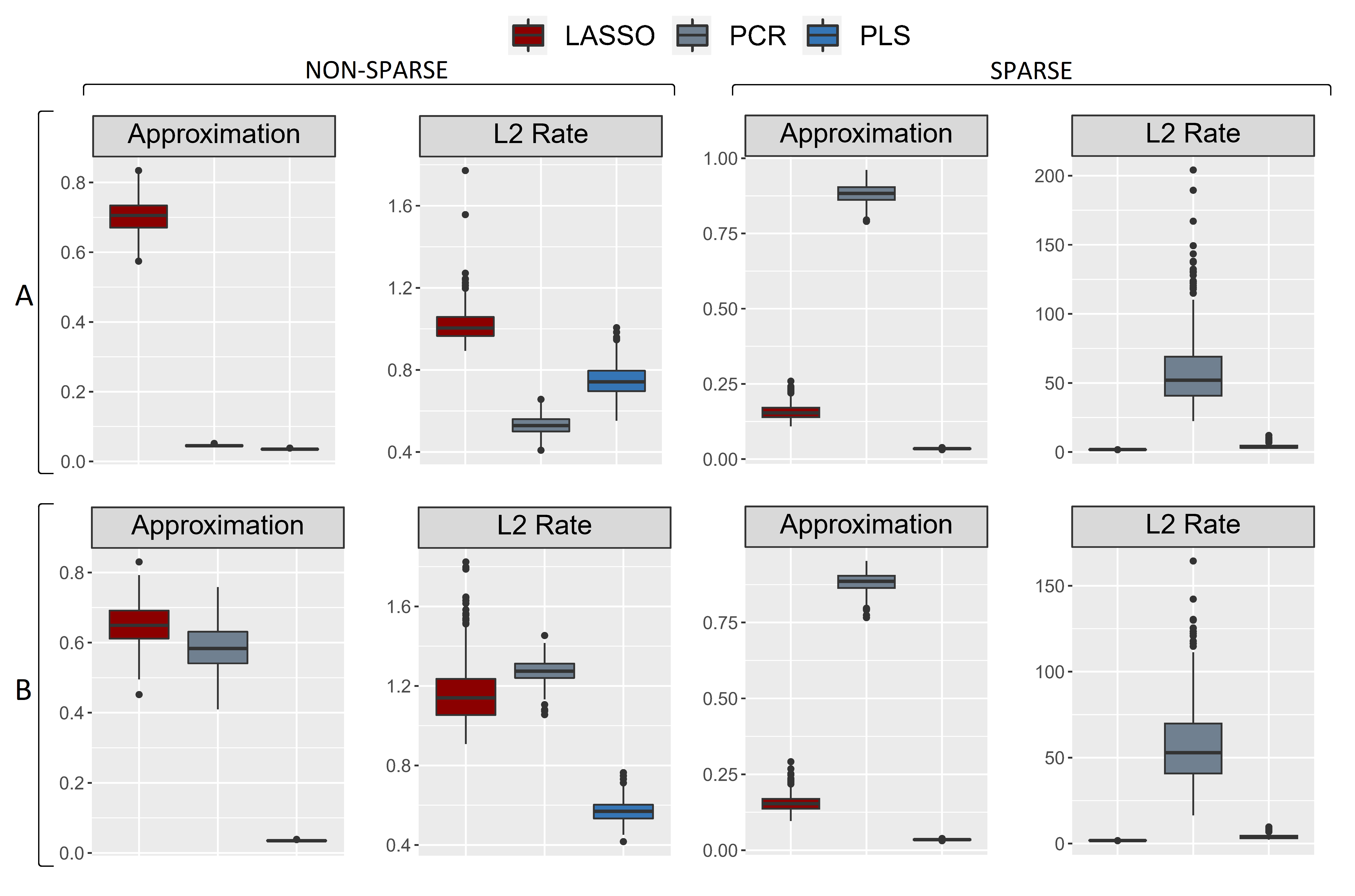
Figure 2: Our simulation study with $n>p$. Relative approximation errors $\|\widehat{\mathbf{y}}_{m}-\mathbf{y}\|_{2}/\|\mathbf{y}\|_{2}$ and relative $L^{2}$ estimation rates $\|\widehat{\bm{\beta}}_{m}-\bm{\beta}_{0}\|_{2}/\|\bm{\beta}_{0}\|_{2}$ in non-sparse (left columns) and sparse (right columns) cases:
A) large noise level $\sigma_{0}=0.1$ (SNR=$10$) and weak irrelevant features $\sigma_{y^{\bot}}=0.1$
B) large noise level $\sigma_{0}=0.1$ (SNR=$10$) and medium irrelevant features $\sigma_{y^{\bot}}=1$

Case $p>n$. We simulate our data with $n=200$ and $p=1000$. We only consider the non-sparse setting. We compare in Figure 3 the approximation errors and the $L^{2}$ estimation rates for low/full rank irrelevant features with $r_{y^{\bot}}\in\{100,900\}$, with large noise level $\sigma_{0}=0.1$ and weak/medium irrelevant features with $\sigma_{y^{\bot}}\in\{0.1,1\}$. Despite the models not being sparse, LASSO still outperforms its competitors in the $L^{2}$ estimation rates. In the low-rank setup, PLS either outperforms or is comparable to PCR, whereas the latter is negatively affected by the strength of the irrelevant features. In the full-rank setup, PLS becomes the worst method in terms of $L^{2}$ estimation rates. Consistently with our main result and our discussion in Remark 2.15, we can see that PLS estimates are driven by the effective rank of the covariance matrix of the features.

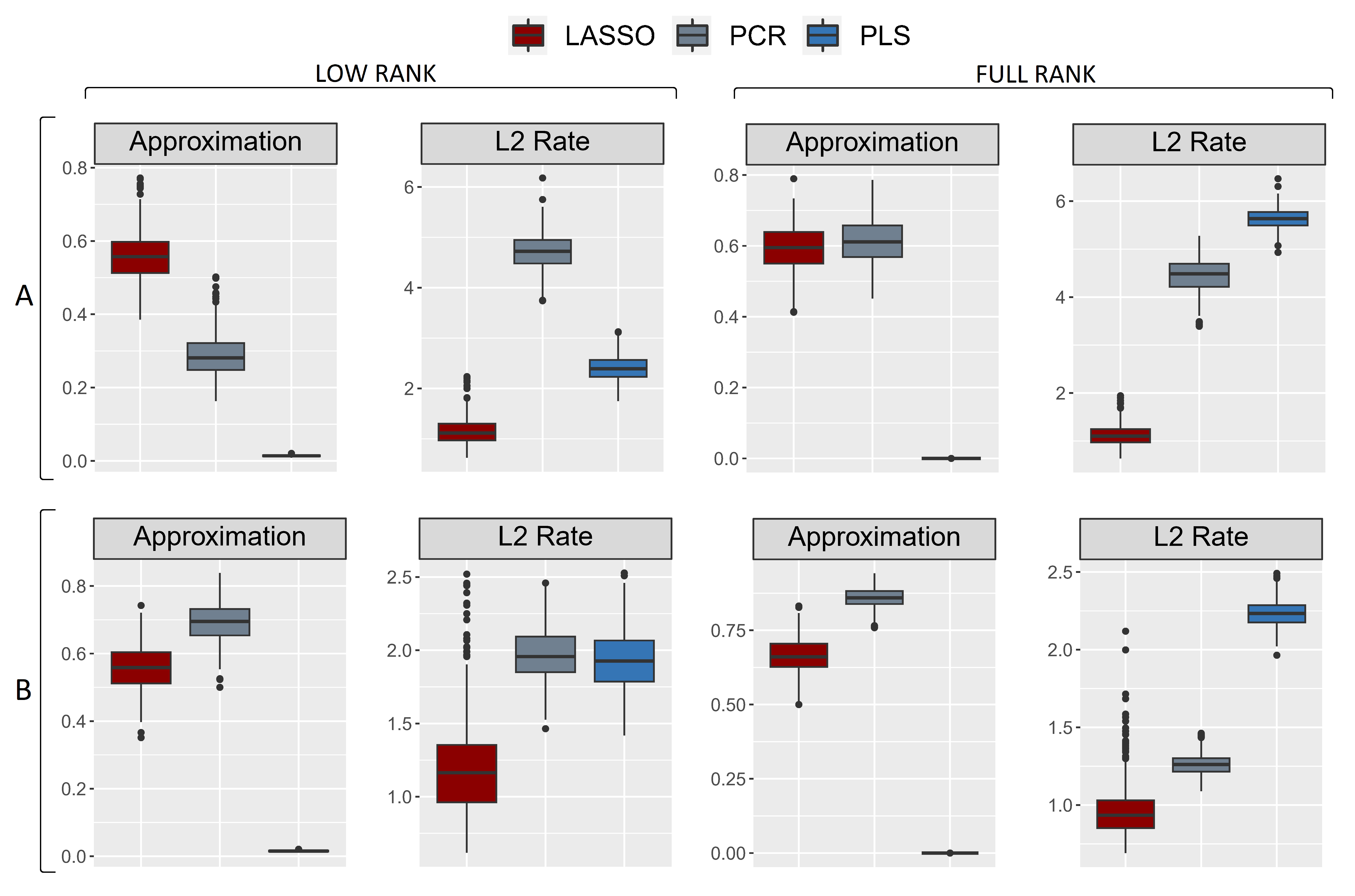
Figure 3: Our simulation study with $p>n$. Relative approximation errors $\|\widehat{\mathbf{y}}_{m}-\mathbf{y}\|_{2}/\|\mathbf{y}\|_{2}$ and relative $L^{2}$ estimation rates $\|\widehat{\bm{\beta}}_{m}-\bm{\beta}_{0}\|_{2}/\|\bm{\beta}_{0}\|_{2}$ in low-rank (left columns) and full-rank (right columns) cases:
A) large noise level $\sigma_{0}=0.1$ (SNR=$10$) and weak irrelevant features $\sigma_{y^{\bot}}=0.1$
B) large noise level $\sigma_{0}=0.1$ (SNR=$10$) and medium irrelevant features $\sigma_{y^{\bot}}=1$

3.2 Real data

We repeat the experiment run by Krivobokova et al. (2012) on the Aqy1 data set. This consists of $n=20.000$ times points and all the $p=2.349$ features. We take the first half of the data as training set $(\mathbf{X}_{train},\mathbf{y}_{train})$ and the remaining half as test set $(\mathbf{X}_{test},\mathbf{y}_{test})$, each consisting of $n/2=10.000$ observations. Since the data has been produced via molecular dynamics simulations, the observations $(\mathbf{x}_{i},y_{i})$, $i=1,\ldots,n$, are not independent nor identically distributed and Singer et al. (2016) show that PLS estimates might be inconsistent if one does not account for this dependence. We thus normalize the training data with an estimated temporal covariance matrix $\widehat{\bm{\Sigma}}\in\mathbb{R}^{n\times n}$ computed according to Klockmann and Krivobokova (2023). That is, we use $(\widetilde{\mathbf{X}}_{train},\widetilde{\mathbf{y}}_{train})$ with $\widetilde{\mathbf{X}}_{train}=\widehat{\bm{\Sigma}}^{-1/2}\mathbf{X}_{train}$ and $\widetilde{\mathbf{y}}_{train}=\widehat{\bm{\Sigma}}^{-1/2}\mathbf{y}_{train}$. The results are shown in Figure 4 and discussed below, PLS seems to the better method overall.

From the training set, we compute the LASSO, PCR and PLS estimators relative to different values of their tuning parameters. For PCR/PLS, we consider estimators $\widehat{\bm{\beta}}_{\widehat{s}}$ corresponding to $\widehat{s}=1,\ldots,15$ latent components. For LASSO, we consider estimators $\widehat{\bm{\beta}}_{\widehat{s}}$ having sparsity parameter $\widehat{s}\leq 15$. Thus, the parameter $\widehat{s}$ measures the degrees of freedom of each estimator $\widehat{\bm{\beta}}_{\widehat{s}}$ obtained via LASSO, PCR or PLS. We also compute the estimated condition number $\widehat{\kappa}_{\widehat{s}}$ of the reduced sample covariance matrix on the training set. To evaluate the models, we compute the correlation between the estimated responses $\widehat{\mathbf{y}}_{\widehat{s}}=\mathbf{X}_{test}\widehat{\bm{\beta}}_{\widehat{s}}$ and the observed response $\mathbf{y}_{test}$ on the test set, together with the relative $L^{2}$-prediction error $\|\widehat{\mathbf{y}}_{\widehat{s}}-\mathbf{y}_{test}\|_{2}/\|\mathbf{y}_{test}\|_{2}$.

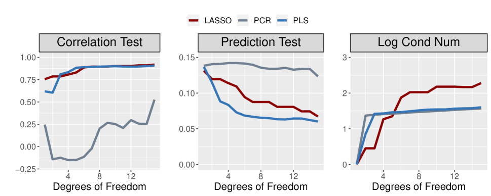
Figure 4: Comparison between LASSO, PCR, PLS on the Aqy1 data set studied by Krivobokova et al. (2012) rescaled according to Klockmann and Krivobokova (2023). From left to right: correlation $Cor(\widehat{\mathbf{y}}_{\widehat{s}},\mathbf{y}_{test})$ between estimated response and true response on test data; relative $L^{2}$-prediction error $\|\widehat{\mathbf{y}}_{\widehat{s}}-\mathbf{y}_{test}\|_{2}/\|\mathbf{y}_{test}\|_{2}$ between estimated response and true response on test data; logarithm (base $10$) of the condition number $\widehat{\kappa}_{\widehat{s}}$ computed from reduced designed matrix on train set.

PLS vs PCR. Figure 4 shows that the condition numbers $\widehat{\kappa}_{\widehat{s}}$ induced by PCR and PLS for all values of $\widehat{s}=1,\ldots,15$ are essentially the same. However, PCR is much worse than PLS in terms of correlation and prediction on the test data. Even with $\widehat{s}=15$, the correlation induced by PCR barely reaches $50\%$, whereas that of PLS is essentially $90\%$.

PLS vs LASSO. In Figure 4 we can see that PLS and LASSO have comparable correlation on the test data, with LASSO being better for small degrees of freedom. On the other hand, PLS outperforms LASSO in terms of prediction on the test data. It appears that LASSO selects active features whose condition number is quite larger than that of the PLS components with same degrees of freedom. This could result in worse recovery of the true (unknown) vector of coefficients, as we have seen in our simulations in Section 3.1.

4 Partial least squares for generalized linear models

We briefly discuss an extension of both our framework and the PLS algorithm to ill-posed generalized-linear-models (GLMs). This is the object of an upcoming work and we only lay down the main ideas.

One can replace the minimization of the population/sample risk in Section 2 with the maximization of an expected/sample log-likelihood. Assumption 2.1 remains the same, whereas in Assumption 2.2 one replaces the latent least-squares with a latent maximum likelihood. Following McCullagh and Nelder (1989), one can devise a population/sample iterative-reweighted-least-squares (IRLS) algorithm to approximate the population/sample maximum likelihood. The convergence rates of such algorithms have been studied by Bissantz et al. (2009). We propose a novel population/sample IRPLS algorithm that is close in spirit to the original extension of PLS by Marx (1996). Its sample version is given below.

Input: $\mathbf{X},\mathbf{y},\widehat{s},\widehat{J},\widehat{\varepsilon}$;

Output: $(\widehat{\bm{\beta}}_{\widehat{s}}^{(j)})_{j\geq 0}$;

$j\leftarrow 0$; $\widehat{D}^{(j)}\leftarrow\infty$; $\widehat{\bm{\beta}}_{\widehat{s}}^{(j)}\leftarrow\mathbf{0}_{p}$;

while  $\widehat{D}^{(j)}>\widehat{\varepsilon}$ and $j<\widehat{J}$ do

       $\widehat{\bm{\eta}}_{\widehat{s}}^{(j)}\leftarrow\mathbf{X}\widehat{\bm{\beta}}_{\widehat{s}}^{(j)}$; $\widehat{\bm{\mu}}_{\widehat{s}}^{(j)}\leftarrow\kappa^{\prime}(\widehat{\bm{\eta}}_{\widehat{s}}^{(j)})$; $\widehat{\mathbf{W}}_{\widehat{s}}^{(j)}\leftarrow\operatorname{diag}(\kappa^{\prime\prime}(\widehat{\bm{\eta}}_{\widehat{s}}^{(j)})$);

       $\mathbf{X}(\widehat{\bm{\eta}}_{\widehat{s}}^{(j)})\leftarrow[\widehat{\mathbf{W}}_{\widehat{s}}^{(j)}]^{1/2}\mathbf{X}$; $\mathbf{r}(\widehat{\bm{\eta}}_{\widehat{s}}^{(j)})\leftarrow[\widehat{\mathbf{W}}_{\widehat{s}}^{(j)}]^{-1/2}(\mathbf{y}-\widehat{\bm{\mu}}_{\widehat{s}}^{(j)})$;

       $\widehat{\bm{\beta}}_{\widehat{s}}^{(j+1)}\leftarrow\widehat{\bm{\beta}}_{\widehat{s}}^{(j)}+\operatorname{PLS}_{\widehat{s}}\left(\widehat{\bm{\Sigma}}_{\mathbf{X}(\widehat{\bm{\eta}}_{\widehat{s}}^{(j)})},\widehat{\bm{\Sigma}}_{\mathbf{X}(\widehat{\bm{\eta}}_{\widehat{s}}^{(j)}),\mathbf{r}(\widehat{\bm{\eta}}_{\widehat{s}}^{(j)})}\right)$;

       $\widehat{D}^{(j)}\leftarrow\widehat{\ell}_{\mathbf{x},y}(\widehat{\bm{\beta}}_{\widehat{s}}^{(j)})-\widehat{\ell}_{\mathbf{x},y}(\widehat{\bm{\beta}}_{\widehat{s}}^{(j+1)})$;

       $j\leftarrow j+1$;

      

end while

fAlgorithm 1 Sample IRPLS

We conjecture that our proving strategy can be extended to derive high-probability $L^{2}$-estimation rates for the sample IRPLS estimator $\widehat{\bm{\beta}}_{\widehat{s}}^{(J)}$, for any fixed $J\geq 0$, with respect to the oracle maximum-likelihood $\bm{\beta}_{0}\in\mathbb{R}^{p}$. The necessary regularity assumptions and the proving strategy are much more technically involved than those we present in this paper for the classical PLS. We conjecture that the convergence rates of Theorem 2.11 hold up to multiplicative constants of the form $(1+c)^{J}$, where $c>0$ is possibly a small constant, and an additional bias term of order $2^{J_{0}-J}$, where $J_{0}\geq 0$ depends on the distribution of the latent model. A bias-variance trade-off arises in the choice of the optimal number $J\geq 0$ of iterations, which in turn might be the symptom of pseudo-convergence. That is to say, the IRPLS algorithm is provably well-behaved only when stopped early. The main difficulty is that each iteration of the IRPLS algorithm is defined conditionally on the previous one, and our PLS perturbation bounds have to be applied conditionally at each step.

Appendix A Auxiliary results

Here we gather all the relevant auxiliary results and provide proofs when necessary.

A.1 Random vectors

Lemma A.1.

Let $\mathbf{x}\in\mathbb{R}^{p}$ be a centered random vector and $y\in\mathbb{R}$ a random variable both with finite second moments. Then, $\mathbb{P}(\mathbf{x}\in\mathcal{R}(\bm{\Sigma}_{\mathbf{x}}))=1$ and $\bm{\Sigma}_{\mathbf{x},y}\in\mathcal{R}(\bm{\Sigma}_{\mathbf{x}})$.

Proof of Lemma A.1.

For the first statement, let $\mathbf{P}\mathbf{P}^{\top}\in\mathbb{R}^{p\times p}$ be the orthogonal projection onto $\mathcal{R}(\bm{\Sigma}_{\mathbf{x}})$, so that $\mathbf{P}\mathbf{P}^{\top}\bm{\Sigma}_{\mathbf{x}}=\bm{\Sigma}_{\mathbf{x}}=\bm{\Sigma}_{\mathbf{x}}\mathbf{P}\mathbf{P}^{\top}$ and $\mathcal{R}(\bm{\Sigma}_{\mathbf{x}})=\mathcal{R}(\mathbf{P}\mathbf{P}^{\top})$. Then, we define the random vector $\mathbf{e}_{\mathbf{x}^{\bot}}:=(\mathbf{I}_{p}-\mathbf{P}\mathbf{P}^{\top})\mathbf{x}\in\mathcal{R}(\bm{\Sigma}_{\mathbf{x}})^{\bot}$ and prove that $\mathbb{P}(\mathbf{e}_{\mathbf{x}^{\bot}}=\mathbf{0}_{p})=1$. For this, compute the covariance matrix

$$\bm{\Sigma}_{\mathbf{e}_{\mathbf{x}^{\bot}}}=\mathbb{E}\left[\mathbf{e}_{\mathbf{x}^{\bot}}\mathbf{e}_{\mathbf{x}^{\bot}}^{\top}\right]=(\mathbf{I}_{p}-\mathbf{P}\mathbf{P}^{\top})\bm{\Sigma}_{\mathbf{x}}(\mathbf{I}_{p}-\mathbf{P}\mathbf{P}^{\top})=\mathbf{0}_{p\times p},$$

thus the vector $\mathbf{e}_{\mathbf{x}^{\bot}}$ is almost surely equal to its expectation $\mathbb{E}[\mathbf{e}_{\mathbf{x}^{\bot}}]=\mathbf{0}_{p}$.

The second statement is a consequence of the first, since $\mathbf{x}=\mathbf{P}\mathbf{P}^{\top}\mathbf{x}$ almost surely and we can write

$$\bm{\Sigma}_{\mathbf{x},y}=\mathbb{E}\left[\mathbf{x}y\right]=\mathbb{E}\left[\mathbf{P}\mathbf{P}^{\top}\mathbf{x}y\right]=\mathbf{P}\mathbf{P}^{\top}\bm{\Sigma}_{\mathbf{x},y}\in\mathcal{R}(\bm{\Sigma}_{\mathbf{x}}).$$

∎

Lemma A.2.

Let $1\leq d\leq p$ be any integers and $\mathbf{P}\in\mathbb{R}^{p\times d}$ any matrix such that $\mathbf{P}^{\top}\mathbf{P}=\mathbf{I}_{d}$. With $\mathbb{B}_{2}^{p}(1)$ the Euclidean unit ball in $\mathbb{R}^{p}$, the possibly degenerate standard Gaussian vector $\mathbf{g}\sim\mathcal{N}(\mathbf{0}_{p},\mathbf{P}\mathbf{P}^{\top})\in\mathbb{R}^{p}$ satisfies $\mathbb{E}[\sup_{\mathbf{v}\in\mathbb{B}_{2}^{p}(1)}|\mathbf{g}^{\top}\mathbf{v}|]\leq\sqrt{2d}$.

Proof of Lemma A.2.

For any $\mathbf{v}\in\mathbb{R}^{p}$, one has $|\mathbf{g}^{\top}\mathbf{v}|\leq\|\mathbf{g}\|_{2}\|\mathbf{v}\|_{2}$. Furthermore, the random variable $\|\mathbf{g}\|_{2}$ is distributed as $\chi_{d}$, which is a chi distribution with $d$ degrees of freedom. Gautschi’s inequality, see Gautschi (1959), guarantees that $\Gamma(x+1)/\Gamma(x+s)<(x+1)^{1-s}$ for all $0<s<1$ and $x>0$. Putting all the above together, we find

$$\mathbb{E}\left[\sup_{\mathbf{v}\in\mathbb{B}_{2}^{p}(1)}|\mathbf{g}^{\top}\mathbf{v}|\right]\leq\mathbb{E}[\|\mathbf{g}\|_{2}]=\mathbb{E}[\chi_{d}]=\sqrt{2}\cdot\frac{\Gamma(\frac{d+1}{2})}{\Gamma(\frac{d}{2})}\leq\sqrt{2}\left(\frac{d+1}{2}\right)^{1-\frac{1}{2}}=\sqrt{d+1}.$$

We conclude the proof with $\sqrt{d+1}\leq\sqrt{2d}$, since $d\geq 1$ is an integer. ∎

A.2 Empirical processes

The following result is a special case of a theorem by Mendelson (2017) applied to non-isotropic vectors. For a centered random vector $\mathbf{x}\in\mathbb{R}^{p}$ with invertible covariance matrix $\bm{\Sigma}_{\mathbf{x}}$, we denote $\widetilde{\mathbf{x}}:=\bm{\Sigma}_{\mathbf{x}}^{-1/2}\mathbf{x}\in\mathbb{R}^{p}$ its isotropic counterpart.

Theorem A.3 (Theorem 1.2 by Mendelson (2017)).

For some integer $p\geq 1$, let $\mathbf{x}\in\mathbb{R}^{p}$ be a subgaussian random vector. Let $\xi\in\mathbb{R}$ be a random variable (not necessarily independent of $\mathbf{x}$) with $\mathbb{E}[|\xi|^{4}]^{1/4}\leq M_{\xi}$. Let $1\leq d\leq p$ be any integer and $\mathbf{P}\in\mathbb{R}^{p\times d}$ any matrix such that $\mathbf{P}^{\top}\mathbf{P}=\mathbf{I}_{d}$. Let $(\mathbf{x}_{i},\xi_{i})_{i=1,\ldots,n}$ be i.i.d. copies of $(\mathbf{x},\xi)$. There exist absolute constants $c_{0},c_{1},c_{2},c_{3},c_{4}$ for which the following holds. With probability at least $1-c_{1}(\log^{4}n)/(16c_{0}^{4}n)-2e^{-4c_{0}^{2}c_{2}d}$, one has

$$\sup_{\mathbf{v}\in\mathbf{P}\mathbf{P}^{\top}\mathbb{B}_{2}^{p}(1)}\left|\frac{1}{\sqrt{n}}\sum_{i=1}^{n}\left(\mathbf{x}_{i}^{\top}\mathbf{v}\xi_{i}-\mathbb{E}[\mathbf{x}^{\top}\mathbf{v}\xi]\right)\right| \leq 4c_{0}^{2}c_{3}\|\widetilde{\mathbf{x}}\|_{\psi_{2}}\|\bm{\Sigma}_{\mathbf{x}}^{1/2}\|_{op}M_{\xi}\sqrt{d}.$$

Proof of Theorem A.3.

Since the variable $\widetilde{\mathbf{x}}=\bm{\Sigma}_{\mathbf{x}}^{-1/2}\mathbf{x}$ is isotropic, and the variables $\mathbf{x}_{i}$ have the same distribution of $\mathbf{x}$, the variables $\widetilde{\mathbf{x}}_{i}=\bm{\Sigma}_{\mathbf{x}}^{-1/2}\mathbf{x}_{i}$ are isotropic. Thus, for all $i=1,\ldots,n$, we rewrite $\mathbf{x}_{i}^{\top}\mathbf{v}\xi_{i}-\mathbb{E}[\mathbf{x}^{\top}\mathbf{v}\xi]=\widetilde{\mathbf{x}}_{i}^{\top}\widetilde{\mathbf{v}}\xi_{i}-\mathbb{E}[\widetilde{\mathbf{x}}^{\top}\widetilde{\mathbf{v}}\xi]$, with $\widetilde{\mathbf{v}}=\bm{\Sigma}_{\mathbf{x}}^{1/2}\mathbf{v}$ having norm $\|\widetilde{\mathbf{v}}\|_{2}\leq\|\bm{\Sigma}_{\mathbf{x}}^{1/2}\|_{op}$ since $\|\mathbf{v}\|_{2}\leq 1$. That is to say, we can bound

$$\sup_{\mathbf{v}\in\mathbf{P}\mathbf{P}^{\top}\mathbb{B}_{2}^{p}(1)}\left|\frac{1}{\sqrt{n}}\sum_{i=1}^{n}\left(\mathbf{x}_{i}^{\top}\mathbf{v}\xi_{i}-\mathbb{E}[\mathbf{x}^{\top}\mathbf{v}\xi]\right)\right|\leq\sup_{\widetilde{\mathbf{v}}\in\mathbf{P}\mathbf{P}^{\top}\mathbb{B}_{2}^{p}(\|\bm{\Sigma}_{\mathbf{x}}^{1/2}\|_{op})}\left|\frac{1}{\sqrt{n}}\sum_{i=1}^{n}\left(\widetilde{\mathbf{x}}_{i}^{\top}\widetilde{\mathbf{v}}\xi_{i}-\mathbb{E}[\widetilde{\mathbf{x}}^{\top}\widetilde{\mathbf{v}}\xi]\right)\right|.$$

We now apply the original Theorem 1.2 by Mendelson (2017) with $q=4$, $w=2c_{0}$, $u=2c_{0}\|\bm{\Sigma}_{\mathbf{x}}^{1/2}\|_{op}$ and subset $V=\mathbf{P}\mathbf{P}^{\top}\mathbb{B}_{2}^{p}(\|\bm{\Sigma}_{\mathbf{x}}^{1/2}\|_{op})\subset\mathbb{R}^{p}$. The supremum of the corresponding degenerate Gaussian process is bounded with Lemma A.2. Thus,

$$\sup_{\widetilde{\mathbf{v}}\in\mathbf{P}\mathbf{P}^{\top}\mathbb{B}_{2}^{p}(\|\bm{\Sigma}_{\mathbf{x}}^{1/2}\|_{op})}\left|\frac{1}{\sqrt{n}}\sum_{i=1}^{n}\left(\widetilde{\mathbf{x}}_{i}^{\top}\widetilde{\mathbf{v}}\xi_{i}-\mathbb{E}[\widetilde{\mathbf{x}}^{\top}\widetilde{\mathbf{v}}\xi]\right)\right| \leq c_{3}uw\|\widetilde{\mathbf{x}}\|_{\psi_{2}}\mathbb{E}[\xi^{4}]^{\frac{1}{4}}\sqrt{d}$$

$$\leq 4c_{0}^{2}c_{3}\|\widetilde{\mathbf{x}}\|_{\psi_{2}}\|\bm{\Sigma}_{\mathbf{x}}^{1/2}\|_{op}M_{\xi}\sqrt{d}$$

with probability at least

$$1-\frac{c_{1}\log^{4}n}{w^{4}n}-2e^{-\frac{c_{2}u^{2}d}{\|\bm{\Sigma}_{\mathbf{x}}^{1/2}\|_{op}^{2}}}=1-\frac{c_{1}\log^{4}n}{16c_{0}^{4}n}-2e^{-4c_{0}^{2}c_{2}d},$$

as required. ∎

We show an immediate corollary of the above result to the case of multivariate multiplier processes.

Corollary A.4.

For some integer $p\geq 1$, let $\mathbf{x}\in\mathbb{R}^{p}$ be a subgaussian random vector. For some integer $k\geq 1$, let $\bm{\xi}\in\mathbb{R}^{k}$ be a random vector (not necessarily independent of $\mathbf{x}$) with $\mathbb{E}[\|\bm{\xi}\|_{\infty}^{4}]^{1/4}\leq M_{\xi}$. Let $1\leq d\leq p$ be any integer and $\mathbf{P}\in\mathbb{R}^{p\times d}$ any matrix such that $\mathbf{P}^{\top}\mathbf{P}=\mathbf{I}_{d}$. Let $(\mathbf{x}_{i},\bm{\xi}_{i})_{i=1,\ldots,n}$ be i.i.d. copies of $(\mathbf{x},\bm{\xi})$. There exist absolute constants $c_{0},c_{1},c_{2},c_{3},c_{4}$ for which the following holds. With probability at least $1-c_{1}(\log^{4}n)/(16c_{0}^{4}n)-2e^{-4c_{0}^{2}c_{2}d}$, one has

$$\sup_{\mathbf{v}\in\mathbf{P}\mathbf{P}^{\top}\mathbb{B}_{2}^{p}(1)}\left\|\frac{1}{\sqrt{n}}\sum_{i=1}^{n}\left(\{\mathbf{x}_{i}^{\top}\mathbf{v}\}\bm{\xi}_{i}-\mathbb{E}[\{\mathbf{x}^{\top}\mathbf{v}\}\bm{\xi}]\right)\right\|_{2}\leq 4c_{0}^{2}c_{3}\|\widetilde{\mathbf{x}}\|_{\psi_{2}}\|\bm{\Sigma}_{\mathbf{x}}^{1/2}\|_{op}M_{\xi}\sqrt{kd}.$$

Proof of Corollary A.4.

One has

$$\left\|\frac{1}{\sqrt{n}}\sum_{i=1}^{n}\left(\{\mathbf{x}_{i}^{\top}\mathbf{v}\}\bm{\xi}_{i}-\mathbb{E}[\{\mathbf{x}^{\top}\mathbf{v}\}\bm{\xi}]\right)\right\|_{2}\leq\sqrt{k}\left\|\frac{1}{\sqrt{n}}\sum_{i=1}^{n}\left(\{\mathbf{x}_{i}^{\top}\mathbf{v}\}\bm{\xi}_{i}-\mathbb{E}[\{\mathbf{x}^{\top}\mathbf{v}\}\bm{\xi}]\right)\right\|_{\infty}.$$

Let $j\in\{1,\ldots,k\}$ be the index realising the maximum in the latter display, since $\mathbb{E}[|\xi_{j}|^{4}]\leq\mathbb{E}[\|\bm{\xi}\|_{\infty}^{4}]\leq M_{\xi}^{4}$, an application of Theorem A.3 gives

$$\sqrt{k}\sup_{\mathbf{v}\in\mathbf{P}\mathbf{P}^{\top}\mathbb{B}_{2}^{p}(1)}\left|\frac{1}{\sqrt{n}}\sum_{i=1}^{n}\left(\{\mathbf{x}_{i}^{\top}\mathbf{v}\}\xi_{i,j}-\mathbb{E}[\{\mathbf{x}^{\top}\mathbf{v}\}\xi_{j}]\right)\right|\leq\sqrt{k}\cdot 4c_{0}^{2}c_{3}\|\widetilde{\mathbf{x}}\|_{\psi_{2}}\|\bm{\Sigma}_{\mathbf{x}}^{1/2}\|_{op}M_{\xi}\sqrt{d},$$

with probability at least $1-c_{1}(\log^{4}n)/(16c_{0}^{4}n)-2e^{-4c_{0}^{2}c_{2}d}$. ∎

The following result is a special case of a corollary in by Kereta and Klock (2021) with $u=4c_{0}^{2}c_{2}\operatorname{rk}(\bm{\Sigma}_{\mathbf{x}})$ and $c_{0},c_{2}$ absolute constants.

Corollary A.5 (Corollary 5 by Kereta and Klock (2021)).

For some integer $p\geq 1$, let $\mathbf{x}\in\mathbb{R}^{p}$ an $L_{x}$-subgaussian random vector. Let $(\mathbf{x}_{i})_{i=1,\ldots,n}$ be i.i.d. copies of $\mathbf{x}$. There exists an absolute constant $c_{5}$ for which the following holds. With probability at least $1-e^{-4c_{0}^{2}c_{2}\operatorname{rk}(\bm{\Sigma}_{\mathbf{x}})}$, for all $n\geq(4c_{0}^{2}c_{2}+1)\operatorname{rk}(\bm{\Sigma}_{\mathbf{x}})$

$$\|\widehat{\bm{\Sigma}}_{\mathbf{x}}-\bm{\Sigma}_{\mathbf{x}}\|_{op}\leq c_{5}L_{x}^{2}\sqrt{\frac{\operatorname{rk}(\bm{\Sigma}_{\mathbf{x}})}{n}}.$$

A.3 Numerical perturbation theory

In this section we provide classical and novel results which are relevant to the theory of deterministic perturbations of least-squares problems.

Lemma A.6.

Let $\mathbf{A}\in\mathbb{R}^{d\times d}$ be any symmetric positive-semidefinite matrix, $\mathbf{b}\in\mathcal{R}(\mathbf{A})$ any vector and $\bm{\zeta}_{ls}:=\mathbf{A}^{+}\mathbf{b}=\operatorname{LS}(\mathbf{A},\mathbf{b})$. Then, $\bm{\zeta}_{ls}\in\mathcal{K}_{r}(\mathbf{A},\mathbf{b})$ with $r:=\deg(p_{\mathbf{A}})$.

Proof of Lemma A.6.

The Cayley-Hamilton theorem, see Theorem 8.1 in Zhang (1997), guarantees that $p_{\mathbf{A}}(\mathbf{A})=\mathbf{0}_{d\times d}$ for $p_{\mathbf{A}}$ the minimum polynomial of $\mathbf{A}$, having degree at most $r:=rk(\mathbf{A})\leq d$. Since $\mathbf{A}^{\top}=\mathbf{A}$, Theorem 3 in Decell (1965) guarantees that the generalized inverse can be represented as $\mathbf{A}^{+}=(\mathbf{A}^{\top})^{\delta}\sum_{k=1}^{r}c_{k-1}\mathbf{A}^{k-1}=(\sum_{k=1}^{r}c_{k-1}\mathbf{A}^{k-1})(\mathbf{A}^{\top})^{\delta}$, with $\delta=0$ if $\mathbf{A}^{+}=\mathbf{A}^{-1}$ and $\delta=1$ otherwise. Notice that $\mathcal{R}(\mathbf{A}^{\top})=\mathcal{R}(\mathbf{A}\mathbf{A}^{+})$ and $\mathbf{b}\in\mathcal{R}(\mathbf{A})$ implies $\mathbf{A}\mathbf{A}^{+}\mathbf{b}=\mathbf{b}$, we find

$$\bm{\zeta}_{ls}=\mathbf{A}^{+}\mathbf{b}\in\operatorname{span}\{\mathbf{A}\mathbf{A}^{+}\mathbf{b},\ldots,\mathbf{A}^{r-1}\mathbf{A}\mathbf{A}^{+}\mathbf{b}\}=\operatorname{span}\{\mathbf{b},\ldots,\mathbf{A}^{r-1}\mathbf{b}\},$$

as required. ∎

Lemma A.7.

Let $1\leq m\leq d$ be any integers, $\mathbf{P}\in\mathbb{R}^{d\times m}$ any matrix with $\mathbf{P}^{\top}\mathbf{P}=\mathbf{I}_{m}$, $\mathbf{A}\in\mathbb{R}^{m\times m}$ any symmetric and positive-definite matrix and $\mathbf{b}\in\mathbb{R}^{m}$ any vector. Let $\widetilde{\mathbf{A}}:=\mathbf{P}\mathbf{A}\mathbf{P}^{\top}\in\mathbb{R}^{d\times d}$ and $\widetilde{\mathbf{b}}:=\mathbf{P}\mathbf{b}$. Then, $\mathcal{K}(\widetilde{\mathbf{A}},\widetilde{\mathbf{b}})=\mathbf{P}\cdot\mathcal{K}(\mathbf{A},\mathbf{b})$. Furthermore, with $\bm{\zeta}_{ls}:=\mathbf{A}^{-1}\mathbf{b}$ and $\widetilde{\bm{\zeta}}_{ls}:=\widetilde{\mathbf{A}}^{+}\widetilde{\mathbf{b}}$, one has $\widetilde{\bm{\zeta}}_{ls}=\mathbf{P}\bm{\zeta}_{ls}$.

Proof of Lemma A.7.

By construction, $rk(\widetilde{\mathbf{A}})=rk(\mathbf{A})=m\leq d$ and $\mathbf{A}$ is invertible. Using that $\mathbf{P}^{\top}\mathbf{P}=\mathbf{I}_{m}$, from the definition we get

$$\mathcal{K}(\widetilde{\mathbf{A}},\widetilde{\mathbf{b}}) =\operatorname{span}\{\widetilde{\mathbf{b}},\widetilde{\mathbf{A}}\widetilde{\mathbf{b}},\ldots,\widetilde{\mathbf{A}}^{d-1}\widetilde{\mathbf{b}}\}$$

$$=\operatorname{span}\{\mathbf{P}\mathbf{b},\mathbf{P}\mathbf{A}\mathbf{P}^{\top}\mathbf{P}\mathbf{b},\ldots,\mathbf{P}\mathbf{A}^{d-1}\mathbf{P}^{\top}\mathbf{P}\mathbf{b}\}$$

$$=\mathbf{P}\cdot\operatorname{span}\{\mathbf{b},\mathbf{A}\mathbf{b},\ldots,\mathbf{A}^{m-1}\mathbf{b}\}$$

$$=\mathbf{P}\cdot\mathcal{K}(\mathbf{A},\mathbf{b}).$$

The second claim is a consequence of Lemma A.6 and the correspondence between Krylov spaces. We provide below a direct alternative proof. First, we check that $\mathbf{P}\mathbf{A}\mathbf{P}^{\top}\cdot\mathbf{P}\mathbf{A}^{-1}\mathbf{P}^{\top}\cdot\mathbf{P}\mathbf{A}\mathbf{P}^{\top}=\mathbf{P}\mathbf{A}\mathbf{P}^{\top}$, meaning that $(\mathbf{P}\mathbf{A}\mathbf{P}^{\top})^{+}=\mathbf{P}\mathbf{A}^{-1}\mathbf{P}^{\top}$. Then,

$$\widetilde{\bm{\zeta}}_{ls} =\widetilde{\mathbf{A}}^{+}\widetilde{\mathbf{b}}=(\mathbf{P}\mathbf{A}\mathbf{P}^{\top})^{+}\mathbf{P}\mathbf{b}=\mathbf{P}\mathbf{A}^{-1}\mathbf{P}^{\top}\mathbf{P}\mathbf{b}=\mathbf{P}\bm{\zeta}_{ls}.$$

∎

Lemma A.8.

Let $\mathbf{A}\in\mathbb{R}^{d\times d}$ be any symmetric positive-semidefinite matrix, $\mathbf{b}\in\mathcal{R}(\mathbf{A})$ any vector. Let $\bm{\Psi}\in\mathbb{R}^{d\times d}$ any matrix such that $\mathbf{A}\bm{\Psi}=\bm{\Psi}\mathbf{A}=\mathbf{0}_{d\times d}$ and $\bm{\Psi}\mathbf{b}=\mathbf{0}_{d}$. Then, with $m:=\dim(\mathcal{K}(\mathbf{A},\mathbf{b}))$ and all $1\leq s\leq d$, one has $\mathcal{K}_{s}(\mathbf{A}+\bm{\Psi},\mathbf{b})=\mathcal{K}_{s\wedge m}(\mathbf{A},\mathbf{b})$.

Proof of Lemma A.8.

By definition,

$$\mathcal{K}_{s}(\mathbf{A}+\bm{\Psi},\mathbf{b}) =\operatorname{span}\{\mathbf{b},(\mathbf{A}+\bm{\Psi})\mathbf{b},\ldots,(\mathbf{A}+\bm{\Psi})^{s-1}\mathbf{b}\}$$

$$=\operatorname{span}\{\mathbf{b},(\mathbf{A}+\bm{\Psi})\mathbf{b},\ldots,(\mathbf{A}^{s-1}+\bm{\Psi}^{s-1})\mathbf{b}\}$$

$$=\operatorname{span}\{\mathbf{b},\mathbf{A}\mathbf{b},\ldots,\mathbf{A}^{s-1}\mathbf{b}\}$$

$$=\mathcal{K}_{s\wedge m}(\mathbf{A},\mathbf{b}).$$

∎

The following result is a classical perturbation bound for least-squares problems by Wei (1989).

Theorem A.9 (Theorem 1.1 by Wei (1989)).

Let $\bm{\zeta}_{ls}:=\operatorname{LS}(\mathbf{A},\mathbf{b})$ be the $L^{2}$-minimum-norm solution of a least-squares problem with $\mathbf{A}\in\mathbb{R}^{p\times p}$ some symmetric and positive semi-definite matrix and $\mathbf{b}\in\mathcal{R}(\mathbf{A})$ some vector. Let $\widetilde{\bm{\zeta}}_{ls}:=\operatorname{LS}(\widetilde{\mathbf{A}},\widetilde{\mathbf{b}})$ be the $L^{2}$-minimum-norm solution of a perturbed least-squares problem with $\widetilde{\mathbf{A}}=\mathbf{A}+\Delta\widetilde{\mathbf{A}}\in\mathbb{R}^{p\times p}$ some symmetric and positive semi-definite matrix and $\widetilde{\mathbf{b}}=\mathbf{b}+\Delta\widetilde{\mathbf{b}}\in\mathcal{R}(\widetilde{\mathbf{A}})$ some vector. Assume that $\operatorname{rk}(\widetilde{\mathbf{A}})=\operatorname{rk}(\mathbf{A})$ and

$$\frac{\|\Delta\widetilde{\mathbf{b}}\|_{2}}{\|\mathbf{b}\|_{2}}\leq\varepsilon,\quad\frac{\|\Delta\widetilde{\mathbf{A}}\|_{op}}{\|\mathbf{A}\|_{op}}\leq\varepsilon,\quad 0\leq\varepsilon\leq\frac{1}{2\cdot\kappa_{2}(\mathbf{A})}.$$

Then,

$$\frac{\|\widetilde{\bm{\zeta}}_{ls}-\bm{\zeta}_{ls}\|_{2}}{\|\bm{\zeta}_{ls}\|_{2}} \leq 5\cdot\kappa_{2}(\mathbf{A})\varepsilon.$$

We recall and adapt the main results from the numerical perturbation theory of Krylov spaces initiated by Carpraux et al. (1994) and later developed by Kuznetsov (1997). It is worth noticing that the whole theory has been developed in terms of perturbation bounds with respect to the Frobenius norm $\|\cdot\|_{F}$ instead of the operator norm $\|\cdot\|_{op}$. However, the choice of metric on the space of square matrices is arbitrary, as long as it is unitary invariant. To see this, notice that all the proofs by Kuznetsov (1997) exploit the properties of orthogonal matrices presented in their Section 4, which are already expressed in terms of operator norms. We provide below the immediate generalization of the main objects from the classical theory to the case of perturbations in operator norm. Let $\mathbf{U}\in\mathbb{R}^{p\times p}$ be some matrix such that $\mathbf{U}^{\top}\mathbf{U}=\mathbf{I}_{p}$, its spectrum $\operatorname{Sp}(\mathbf{U})=\{\lambda_{1}(\mathbf{U}),\ldots,\lambda_{p}(\mathbf{U})\}$ is a subset of the unit circle. That is, one can write $\lambda_{j}(\mathbf{U})=e^{i\omega_{j}(\mathbf{U})}$ for some $\omega_{j}(\mathbf{U})\in\mathbb{R}$ and order these values as $-\pi\leq\omega_{1}(\mathbf{U})\leq\ldots\leq\omega_{p}(\mathbf{U})<\pi$. The following is an adaptation of Definition 2.1 by Kuznetsov (1997) to suit our needs, we denote

$$\rho(\mathbf{U}):=\max\left\{|\omega_{j}|:e^{i\omega_{j}}\in\operatorname{Sp}(\mathbf{U}),0<\omega_{j}<\pi\right\},$$

where the bound on the interval $(0,\pi)$ is justified by the fact that the eigenvalues of $\mathbf{U}$ consist of complex-conjugate pairs. As for the original definition, we remove the real eigenvalues $\{\pm 1\}$. Let $\mathcal{B}$ and $\widetilde{\mathcal{B}}$ be two $m$-dimensional subspaces of $\mathbb{R}^{p}$, and let $\mathbf{B}\in\mathbb{R}^{p\times m}$ and $\widetilde{\mathbf{B}}\in\mathbb{R}^{p\times m}$ some orthonormal basis of $\mathcal{B}$ and $\widetilde{\mathcal{B}}$ respectively. Then, there exists some matrix $\mathbf{U}\in\mathbb{R}^{p\times p}$ with $\mathbf{U}^{\top}\mathbf{U}=\mathbf{I}_{p}$ such that $\widetilde{\mathbf{B}}=\mathbf{U}\mathbf{B}$. With the above, we define

$$d(\mathbf{B},\widetilde{\mathbf{B}}):=\inf_{\mathbf{U}}\rho(\mathbf{U}),\quad d(\mathcal{B},\widetilde{\mathcal{B}}):=\inf_{\mathbf{B},\widetilde{\mathbf{B}}}d(\mathbf{B},\widetilde{\mathbf{B}}),$$ (5)

where the first infimum is taken over all possible orthonormal matrices such that $\widetilde{\mathbf{B}}=\mathbf{U}\mathbf{B}$ and the second infimum is taken over all possible orthonormal bases $\mathbf{B},\widetilde{\mathbf{B}}$ of $\mathcal{B},\widetilde{\mathcal{B}}$. This is the same as Definition 2.2 by Kuznetsov (1997), the only difference being the definition of spectral radius $\rho(\mathbf{U})$ in the previous display.

Lemma A.10.

For some $1\leq m\leq p$, let $\mathcal{B}\subseteq\mathbb{R}^{p}$ and $\widetilde{\mathcal{B}}\subseteq\mathbb{R}^{p}$ be two orthogonal $m$-dimensional subspaces. Then, $d(\mathcal{B},\widetilde{\mathcal{B}})=\pi/2$.

Proof of Lemma A.10.

Let $\mathbf{B}=(\mathbf{v}_{1}|\cdots|\mathbf{v}_{m})\in\mathbb{R}^{p\times m}$ and $\widetilde{\mathbf{B}}=(\widetilde{\mathbf{v}}_{1}|\cdots|\widetilde{\mathbf{v}}_{m})\in\mathbb{R}^{p\times m}$ be any two orthonormal basis of $\mathcal{B}$ and $\widetilde{\mathcal{B}}$, respectively. By orthogonality, the vectors $\mathbf{v}_{i}$ and $\widetilde{\mathbf{v}}_{j}$ are linearly independent for all $i,j=1,\ldots,m$. Thus, there exist vectors $\mathbf{w}_{1},\ldots,\mathbf{w}_{p-2m}$ such that $(\mathbf{v}_{1}|\cdots|\mathbf{v}_{m}|\widetilde{\mathbf{v}}_{1}|\cdots|\widetilde{\mathbf{v}}_{m}|\mathbf{w}_{1}|\cdots|\mathbf{w}_{p-2m})\in\mathbb{R}^{p\times p}$ is an orthonormal basis of $\mathbb{R}^{p}$. Now, among all possible orthogonal transformations $\mathbf{U}\in\mathbb{R}^{p\times p}$ such that $\widetilde{\mathbf{B}}=\mathbf{U}\mathbf{B}$, the ones achieving the smallest $\rho(\mathbf{U})$ in Equation (5) are those such that $\mathbf{U}\mathbf{w}_{i}=\pm\mathbf{w}_{i}$ for all $i=1,\ldots,p-2m$. Any such matrix is then a pairwise permutation matrix that swaps positions of $\mathbf{v}_{i}$ and $\widetilde{\mathbf{v}}_{i}$ in the original basis of $\mathbb{R}^{p}$. The spectrum $\operatorname{Sp}(\mathbf{U})$ of such a matrix consists of the eigenvalue $\pm 1$ corresponding to the fixed points and the complex unit root $i=e^{i\pi/2}$. From Equation (5), we get

$$d\left(\mathcal{B},\widetilde{\mathcal{B}}\right)=\min_{\widetilde{\mathbf{B}},\mathbf{B}}\ \min_{\mathbf{U}:\widetilde{\mathbf{B}}=\mathbf{U}\mathbf{B}}\rho(\mathbf{U})=\min_{\widetilde{\mathbf{B}},\mathbf{B}}\ \min_{\mathbf{U}:\widetilde{\mathbf{B}}=\mathbf{U}\mathbf{B}}\max\left\{\left|\frac{\pi}{2}\right|:e^{i\pi/2}\in\operatorname{Sp}(\mathbf{U})\right\}=\frac{\pi}{2}.$$

∎

Lemma A.11 (Lemma 1 by Carpraux et al. (1994)).

Let $\mathbf{B},\widetilde{\mathbf{B}}$ be orthonormal bases of $\mathcal{B},\widetilde{\mathcal{B}}$ such that $\widetilde{\mathbf{B}}=(\mathbf{I}_{p}+\bm{\Delta}+O(\|\bm{\Delta}\|_{op}^{2}))\mathbf{B}$ for some $\|\bm{\Delta}\|_{op}\ll 1$. Then, at the first order in $\|\bm{\Delta}\|_{op}\ll 1$, one has

$$d(\mathbf{B},\widetilde{\mathbf{B}})=\inf_{\bm{\Delta}}\|\bm{\Delta}\|_{op},$$

where the infimum is taken over all matrices $\bm{\Delta}\in\mathbb{R}^{p\times p}$ such that $\|\bm{\Delta}\|_{op}\ll 1$, $\bm{\Delta}^{\top}=-\bm{\Delta}$ and $\widetilde{\mathbf{B}}=(\mathbf{I}_{p}+\bm{\Delta}+O(\|\bm{\Delta}\|_{op}^{2}))\mathbf{B}$.

We always consider $\mathbf{A}\in\mathbb{R}^{p\times p}$ some symmetric and positive semi-definite matrix and $\mathbf{b}\in\mathcal{R}(\mathbf{A})$ some vector, together with a Krylov space $\mathcal{K}_{m}=\mathcal{K}_{m}(\mathbf{A},\mathbf{b})$ of full dimension, that is $m=\dim(\mathcal{K}_{m}(\mathbf{A},\mathbf{b}))$ for some $1\leq m\leq p$. We are interested in all perturbations $\widetilde{\mathbf{A}}=\mathbf{A}+\Delta\widetilde{\mathbf{A}}\in\mathbb{R}^{p\times p}$ some symmetric and positive semi-definite matrix and $\widetilde{\mathbf{b}}=\mathbf{b}+\Delta\widetilde{\mathbf{b}}\in\mathcal{R}(\widetilde{\mathbf{A}})$ some vector such that the perturbed Krylov space $\widetilde{\mathcal{K}}_{m}=\mathcal{K}_{m}(\widetilde{\mathbf{A}},\widetilde{\mathbf{b}})$ has full dimension, that is $m=\dim(\mathcal{K}_{m}(\widetilde{\mathbf{A}},\widetilde{\mathbf{b}}))$. We denote $\mathbf{K}_{m}\in\mathbb{R}^{p\times m}$ and $\widetilde{\mathbf{K}}_{m}\in\mathbb{R}^{p\times m}$ any natural orthonormal bases of $\mathcal{K}_{m}(\mathbf{A},\mathbf{b})$ and $\mathcal{K}_{m}(\widetilde{\mathbf{A}},\widetilde{\mathbf{b}})$, in the sense of Definition 2 by Carpraux et al. (1994). Notice that these bases are unique up to their signs and can be computed, for example, with the Arnoldi iteration devised by Arnoldi (1951). When $\widetilde{\mathbf{A}}=\mathbf{A}$ and $\widetilde{\mathbf{b}}=\mathbf{b}$, one can always find some orthonormal matrix $\mathbf{U}\in\mathbb{R}^{p\times p}$ having spectrum $\operatorname{Sp}(\mathbf{U})=\{\pm 1\}$ and such that $\widetilde{\mathbf{K}}_{m}=\mathbf{U}\mathbf{K}_{m}$, so that $d(\mathbf{K}_{m},\widetilde{\mathbf{K}}_{m})=0$ even though $\mathbf{K}_{m}\neq\widetilde{\mathbf{K}}_{m}$ (the identity holds up to the signs of the columns). Consider an arbitrary perturbation and recall that Lemma A.7 implies that Krylov spaces are invariant under orthonormal transformations. Thus, there exist $\mathbf{V}_{m}=(\mathbf{K}_{m}|\mathbf{K}_{m^{\bot}})\in\mathbb{R}^{p\times p}$ and $\widetilde{\mathbf{V}}_{m}=(\widetilde{\mathbf{K}}_{m}|\widetilde{\mathbf{K}}_{m^{\bot}})\in\mathbb{R}^{p\times p}$ both orthonormal bases of $\mathbb{R}^{p}$ such that $\mathbf{G}_{m}=\mathbf{V}_{m}^{\top}\mathbf{K}_{m}$ and $\widetilde{\mathbf{G}}_{m}=\widetilde{\mathbf{V}}_{m}^{\top}\widetilde{\mathbf{K}}_{m}$ are the natural orthonormal bases of $\mathcal{K}_{m}(\mathbf{H}_{m},\mathbf{e}_{1})$ and $\mathcal{K}_{m}(\widetilde{\mathbf{H}}_{m},\mathbf{e}_{1})$ with $\mathbf{e}_{1}\in\mathbb{R}^{p}$ the first vector of the canonical basis and both $\mathbf{H}_{m}=\mathbf{V}_{m}^{\top}\mathbf{A}\mathbf{V}_{m}\in\mathbb{R}^{p\times p}$, $\widetilde{\mathbf{H}}_{m}=\widetilde{\mathbf{V}}_{m}^{\top}\widetilde{\mathbf{A}}\widetilde{\mathbf{V}}_{m}\in\mathbb{R}^{p\times p}$ tridiagonal symmetric (Hessenberg symmetric) matrices. In particular, one can always reduce the problem to perturbations of Krylov spaces having same vector $\widetilde{\mathbf{b}}=\mathbf{b}$ and tridiagonal symmetric matrices. We denote the set of such perturbations by $\mathcal{D}_{m}(\mathbf{H})$ and the size of the perturbation by $\Delta(\widetilde{\mathbf{H}}):=\|\Delta\widetilde{\mathbf{H}}\|_{op}/\|\mathbf{H}\|_{op}$, we define

$$\kappa_{b}(\mathbf{G}_{m}) :=\inf_{\varepsilon>0}\ \sup_{\widetilde{\mathbf{H}}\in\mathcal{D}_{m}(\mathbf{H})\ :\ \Delta(\widetilde{\mathbf{H}})\leq\varepsilon}\frac{d(\mathbf{G}_{m},\widetilde{\mathbf{G}}_{m})}{\Delta(\widetilde{\mathbf{H}})},\quad\kappa_{2}(\mathcal{K}_{m}(\mathbf{H},\mathbf{e}_{1})):=\min_{\mathbf{G}_{m}}\kappa_{b}(\mathbf{G}_{m}),$$ (6)

where the last minimum is taken over all the $2^{m}$ possible natural bases of $\mathcal{K}_{m}(\mathbf{H},\mathbf{e}_{1})$. Our definition of $\kappa_{b}(\mathbf{G}_{m})$ matches Definition 3 by  Carpraux et al. (1994), for which the reduction to the Hessenberg case (tridiagonal symmetric for us) is given in their Theorem 1.

Theorem A.12 (Theorem 3.1 by Kuznetsov (1997)).

Let $\mathbf{H}\in\mathbb{R}^{p\times p}$ be a symmetric tridiagonal matrix and $m=\dim(\mathcal{K}_{m}(\mathbf{H},\mathbf{e}_{1}))$ for some $1\leq m\leq p$. Assume $\mathbf{H}(t)\in\mathbb{R}^{p\times p}$ is a continuously differentiable matrix function such that

$$\mathbf{H}(0)=\mathbf{H},\quad\left\|\frac{d\mathbf{H}(t)}{dt}\right\|_{op}\leq\nu\|\mathbf{H}(t)\|_{op},$$

for some $0<\nu<1$. Let $\mathbf{V}_{m}(t)\in\mathbb{R}^{p\times p}$ be the orthogonal matrix defined as the solution of the Cauchy-problem in Equations (3.1) - (3.3) by Kuznetsov (1997). For all $\mathbf{G}_{m}\in\mathbb{R}^{p\times m}$ natural orthonormal bases of $\mathcal{K}_{m}(\mathbf{H},\mathbf{e}_{1})$ and

$$0\leq t\leq\frac{1}{16\nu\kappa_{b}(\mathbf{G}_{m})(\kappa_{b}(\mathbf{G}_{m})+1)},$$

one has

$$\|\mathbf{V}_{m}^{\top}(t)\mathbf{G}_{m}-\mathbf{G}_{m}\|_{op}\leq 2\kappa_{b}(\mathbf{G}_{m})\nu t.$$

Proof of Theorem A.12.

We slightly adapt the proof of Theorem 3.1 by Kuznetsov (1997). Their Equation (3.7) becomes for us

$$\delta_{m}(t)=2\sin\left(\frac{\int_{0}^{t}\|\mathbf{X}_{m}(\xi)\|_{op}d\xi}{2}\right),\quad\rho_{m}(t)=\left\{2\delta_{m}(t)+t\nu[1+\delta_{m}(t)]\right\}\|\mathbf{H}\|_{op}.$$

Using that $\|\mathbf{H}(t)-\mathbf{H}\|_{op}=\|\int_{0}^{t}\frac{d}{d\xi}\mathbf{X}(\xi)d\xi\|_{op}\leq t\nu\|\mathbf{H}\|_{op}$, one recovers their bound $\|\mathbf{Z}_{m}(t)-\mathbf{H}\|_{op}\leq\rho_{m}(t)$. The remainder of the proof proceeds as in the original reference. ∎

Theorem A.13 (Theorem 3.3 by Kuznetsov (1997)).

Let $\mathbf{A}\in\mathbb{R}^{p\times p}$ be some symmetric and positive semi-definite matrix and $\mathbf{b}\in\mathcal{R}(\mathbf{A})$ some vector. Let $\widetilde{\mathbf{A}}=\mathbf{A}+\Delta\widetilde{\mathbf{A}}\in\mathbb{R}^{p\times p}$ be some symmetric and positive semi-definite matrix and $\widetilde{\mathbf{b}}=\mathbf{b}+\Delta\widetilde{\mathbf{b}}\in\mathcal{R}(\widetilde{\mathbf{A}})$ some vector. Let $\mathbf{K}_{m}\in\mathbb{R}^{p\times m}$ be any natural orthonormal basis of $\mathcal{K}_{m}=\mathcal{K}_{m}(\mathbf{A},\mathbf{b})$ for some $1\leq m\leq p$. Assume that $m=\dim(\mathcal{K}_{m}(\mathbf{A},\mathbf{b}))=\dim(\mathcal{K}_{m}(\widetilde{\mathbf{A}},\widetilde{\mathbf{b}}))$ and

$$\frac{\|\Delta\widetilde{\mathbf{A}}\|_{op}}{\|\mathbf{A}\|_{op}}\leq\varepsilon,\quad\frac{\|\Delta\widetilde{\mathbf{b}}\|_{2}}{\|\mathbf{b}\|_{2}}\leq\varepsilon,\quad 0\leq\varepsilon\leq\frac{1}{64\kappa_{b}(\mathbf{K}_{m})(\kappa_{b}(\mathbf{K}_{m})+1)}.$$

Then, there exists a natural orthonormal basis $\widetilde{\mathbf{K}}_{m}\in\mathbb{R}^{p\times m}$ of $\widetilde{\mathcal{K}}_{m}=\mathcal{K}_{m}(\widetilde{\mathbf{A}},\widetilde{\mathbf{b}})$ such that

$$\|\widetilde{\mathbf{K}}_{m}-\mathbf{K}_{m}\|_{op}\leq 11\kappa_{b}(\mathbf{K}_{m})\varepsilon.$$

Proof of Theorem A.13.

We slightly improve the proof of Theorem 3.3 by Kuznetsov (1997). Define the continuously differentiable matrix function $\mathbf{A}(t):=\mathbf{A}+(\widetilde{\mathbf{A}}-\mathbf{A})t\in\mathbb{R}^{p\times p}$ so that $\mathbf{A}(0)=\mathbf{A}$ and $\mathbf{A}(1)=\widetilde{\mathbf{A}}$ and $\|\frac{d\mathbf{A}(t)}{dt}\|_{op}=\|\Delta\widetilde{\mathbf{A}}\|_{op}\leq\varepsilon\|\mathbf{A}\|_{op}$. One can find $\mathbf{V}\in\mathbb{R}^{p\times p}$ and $\widetilde{\mathbf{V}}\in\mathbb{R}^{p\times p}$ orthonormal matrices such that $\|\mathbf{V}-\widetilde{\mathbf{V}}\|_{2}\leq\sqrt{2}\varepsilon$ and define Hessenberg matrices $\mathbf{H}=\mathbf{V}^{\top}\mathbf{A}(0)\mathbf{V}$ and $\widetilde{\mathbf{H}}=\widetilde{\mathbf{V}}^{\top}\mathbf{A}(1)\widetilde{\mathbf{V}}$. One can check that $\|\widetilde{\mathbf{H}}-\mathbf{H}\|_{op}\leq(2\sqrt{2}+1)\|\mathbf{H}\|_{op}\varepsilon\leq 4\|\mathbf{H}\|_{op}\varepsilon$. The assumptions of Theorem A.12 hold for $t=1$ and $\nu=4\varepsilon$, thus, with suitable bases $\mathbf{G}_{m}$ and $\widetilde{\mathbf{G}}_{m}$ of $\mathcal{K}_{m}(\mathbf{H},\mathbf{e}_{1})$ and $\mathcal{K}_{m}(\widetilde{\mathbf{H}},\mathbf{e}_{1})$ one has $\|\widetilde{\mathbf{G}}_{m}-\mathbf{G}_{m}\|_{op}\leq 8\kappa_{b}(\mathbf{G}_{m})\varepsilon$. One concludes the proof for the bases $\mathbf{K}_{m}$ and $\widetilde{\mathbf{K}}_{m}$ by writing

$$\|\widetilde{\mathbf{K}}_{m}-\mathbf{K}_{m}\|_{op}=\|\widetilde{\mathbf{V}}\widetilde{\mathbf{G}}_{m}-\mathbf{V}\mathbf{G}_{m}\|_{op}\leq\|\mathbf{V}-\widetilde{\mathbf{V}}\|_{2}+\|\widetilde{\mathbf{G}}_{m}-\mathbf{G}_{m}\|_{op}\leq 11\kappa_{b}(\mathbf{K}_{m})\varepsilon.$$

∎

The next result is a combination of the proof of Theorem 3.3 by Kuznetsov (1997), together with one of its corollaries.

Corollary A.14 (Corollary 2 in Kuznetsov (1997)).

Under the assumptions of Theorem A.13, let $\mathbf{A}_{m}=\mathbf{K}_{m}^{\top}\mathbf{A}\mathbf{K}_{m}\in\mathbb{R}^{m\times m}$, $\mathbf{b}_{m}=\mathbf{K}_{m}^{\top}\mathbf{b}\in\mathbb{R}^{m}$ be the projected matrix and vector relative to the orthonormal basis $\mathbf{K}_{m}\in\mathbb{R}^{p\times m}$ and $\widetilde{\mathbf{A}}_{m}=\widetilde{\mathbf{K}}_{m}^{\top}\widetilde{\mathbf{A}}\widetilde{\mathbf{K}}_{m}\in\mathbb{R}^{m\times m}$, $\widetilde{\mathbf{b}}_{m}=\widetilde{\mathbf{K}}_{m}^{\top}\widetilde{\mathbf{b}}\in\mathbb{R}^{m}$ be the projected matrix and vector relative to the orthonormal basis $\widetilde{\mathbf{K}}_{m}\in\mathbb{R}^{p\times m}$. Then,

$$\frac{\|\widetilde{\mathbf{b}}_{m}-\mathbf{b}_{m}\|_{2}}{\|\mathbf{b}_{m}\|_{2}}\leq 2\varepsilon,\quad\frac{\|\widetilde{\mathbf{A}}_{m}-\mathbf{A}_{m}\|_{op}}{\|\mathbf{A}_{m}\|_{op}}\leq 24\cdot\kappa_{b}(\mathbf{K}_{m})\|\mathbf{A}\|_{op}\|\mathbf{A}_{m}\|_{op}^{-1}\varepsilon.$$

The following is our novel perturbation bound for PLS solutions. It shows that, as long as the perturbation is sufficiently small, the relative approximation error of the perturbed PLS solution is proportional to the size of the perturbation and the condition number of the unperturbed Krylov space.

Theorem A.15.

Let $\bm{\zeta}_{pls,m}:=\operatorname{PLS}(\mathbf{A},\mathbf{b},m)$ be the PLS solution with parameter $1\leq m\leq p$ computed from $\mathbf{A}\in\mathbb{R}^{p\times p}$ some symmetric and positive semi-definite matrix and $\mathbf{b}\in\mathcal{R}(\mathbf{A})$ some vector. Let $\widetilde{\bm{\zeta}}_{pls,m}:=\operatorname{PLS}(\widetilde{\mathbf{A}},\widetilde{\mathbf{b}},m)$ be the PLS solution with parameter $m$ computed from $\widetilde{\mathbf{A}}=\mathbf{A}+\Delta\widetilde{\mathbf{A}}\in\mathbb{R}^{p\times p}$ some symmetric and positive semi-definite matrix and $\widetilde{\mathbf{b}}=\mathbf{b}+\Delta\widetilde{\mathbf{b}}\in\mathcal{R}(\widetilde{\mathbf{A}})$ some vector. Let $\mathbf{K}_{m}\in\mathbb{R}^{p\times m}$ be any natural orthonormal basis of $\mathcal{K}_{m}(\mathbf{A},\mathbf{b})$ and $C_{m}:=64\cdot\kappa_{b}(\mathbf{K}_{m})(\kappa_{b}(\mathbf{K}_{m})+1)$, $D_{m}:=48\cdot\kappa_{b}(\mathbf{K}_{m})\|\mathbf{A}\|_{op}\|\mathbf{A}_{m}^{-1}\|_{op}$. Assume that $m=\dim(\mathcal{K}_{m}(\mathbf{A},\mathbf{b}))=\dim(\mathcal{K}_{m}(\widetilde{\mathbf{A}},\widetilde{\mathbf{b}}))$ and

$$\frac{\|\Delta\widetilde{\mathbf{b}}\|_{2}}{\|\mathbf{b}\|_{2}}\leq\varepsilon,\quad\frac{\|\Delta\widetilde{\mathbf{A}}\|_{op}}{\|\mathbf{A}\|_{op}}\leq\varepsilon,\quad 0\leq\varepsilon\leq\frac{1}{C_{m}\vee D_{m}}.$$

Then,

$$\frac{\|\widetilde{\bm{\zeta}}_{pls,m}-\bm{\zeta}_{pls,m}\|_{2}}{\|\bm{\zeta}_{pls,m}\|_{2}}\leq 120\cdot\kappa_{b}(\mathbf{K}_{m})\left(\|\mathbf{A}\|_{op}\|\mathbf{A}_{m}\|_{op}^{-1}+1\right)\varepsilon.$$

Proof of Theorem A.15.

Since the assumptions of Theorem A.13 are satisfied, take the natural basis $\widetilde{\mathbf{K}}_{m}\in\mathbb{R}^{p\times m}$ of $\widetilde{\mathcal{K}}_{m}(\widetilde{\mathbf{A}},\widetilde{\mathbf{b}})$ in the statement. Let $\mathbf{P}_{m}:=\mathbf{K}_{m}\mathbf{K}_{m}^{\top}\in\mathbb{R}^{p\times p}$ and $\widetilde{\mathbf{P}}_{m}:=\widetilde{\mathbf{K}}_{m}\widetilde{\mathbf{K}}_{m}^{\top}\in\mathbb{R}^{p\times p}$ the corresponding orthogonal projections onto the Krylov spaces. By definition of PLS solution and Lemma A.7, we write

$$\bm{\zeta}_{pls,m} =\operatorname{LS}\left(\mathbf{P}_{m}\mathbf{A}\mathbf{P}_{m},\mathbf{P}_{m}\mathbf{b}\right)=\mathbf{K}_{m}\cdot\operatorname{LS}\left(\mathbf{A}_{m},\mathbf{b}_{m}\right),$$

$$\widetilde{\bm{\zeta}}_{pls,m} =\operatorname{LS}(\widetilde{\mathbf{P}}_{m}\widetilde{\mathbf{A}}\widetilde{\mathbf{P}}_{m},\widetilde{\mathbf{P}}_{m}\widetilde{\mathbf{b}})=\widetilde{\mathbf{K}}_{m}\cdot\operatorname{LS}(\widetilde{\mathbf{A}}_{m},\widetilde{\mathbf{b}}_{m}),$$

where $\mathbf{A}_{m}=\mathbf{K}_{m}^{\top}\mathbf{A}\mathbf{K}_{m}\in\mathbb{R}^{m\times m}$, $\mathbf{b}_{m}=\mathbf{K}_{m}^{\top}\mathbf{b}\in\mathbb{R}^{m}$ and $\widetilde{\mathbf{A}}_{m}=\widetilde{\mathbf{K}}_{m}^{\top}\widetilde{\mathbf{A}}\widetilde{\mathbf{K}}_{m}\in\mathbb{R}^{m\times m}$, $\widetilde{\mathbf{b}}_{m}=\widetilde{\mathbf{K}}_{m}^{\top}\widetilde{\mathbf{b}}\in\mathbb{R}^{m}$. We denote the projected least-squares solutions $\bm{\alpha}_{ls,m}:=\operatorname{LS}(\mathbf{A}_{m},\mathbf{b}_{m})=\mathbf{A}_{m}^{-1}\mathbf{b}_{m}$ and $\widetilde{\bm{\alpha}}_{ls,m}:=\operatorname{LS}(\widetilde{\mathbf{A}}_{m},\widetilde{\mathbf{b}}_{m})=\widetilde{\mathbf{A}}_{m}^{-1}\widetilde{\mathbf{b}}_{m}$. Then, we can bound

$$\|\widetilde{\bm{\zeta}}_{pls,m}-\bm{\zeta}_{pls,m}\|_{2} =\|\widetilde{\mathbf{K}}_{m}\widetilde{\bm{\alpha}}_{ls,m}-\mathbf{K}_{m}\bm{\alpha}_{ls,m}\|_{2}$$

$$\leq\|\widetilde{\mathbf{K}}_{m}(\widetilde{\bm{\alpha}}_{ls,m}-\bm{\alpha}_{ls,m})\|_{2}+\|(\widetilde{\mathbf{K}}_{m}-\mathbf{K}_{m})\bm{\alpha}_{ls,m}\|_{2}$$

$$\leq\|\widetilde{\bm{\alpha}}_{ls,m}-\bm{\alpha}_{ls,m}\|_{2}+\|\widetilde{\mathbf{K}}_{m}-\mathbf{K}_{m}\|_{op}\|\bm{\alpha}_{ls,m}\|_{2}.$$

With $\varepsilon_{m}:=24\cdot\kappa_{b}(\mathbf{K}_{m})\|\mathbf{A}\|_{op}\|\mathbf{A}_{m}\|_{op}^{-1}\varepsilon$, an application of Corollary A.14 gives

$$\frac{\|\widetilde{\mathbf{b}}_{m}-\mathbf{b}_{m}\|_{2}}{\|\mathbf{b}_{m}\|_{2}}\leq 2\varepsilon\leq\varepsilon_{m},\quad\frac{\|\widetilde{\mathbf{A}}_{m}-\mathbf{A}_{m}\|_{op}}{\|\mathbf{A}_{m}\|_{op}}\leq 24\cdot\frac{\kappa_{b}(\mathbf{K}_{m})\|\mathbf{A}\|_{op}}{\|\mathbf{A}_{m}\|_{op}}\cdot\varepsilon\leq\varepsilon_{m}.$$

By assumption, $\varepsilon\leq D_{m}^{-1}$ and so

$$\varepsilon_{m}=24\cdot\kappa_{b}(\mathbf{K}_{m})\|\mathbf{A}\|_{op}\|\mathbf{A}_{m}\|_{op}^{-1}\varepsilon\leq\frac{1}{2\cdot\kappa_{2}(\mathbf{A}_{m})},$$

meaning that the assumptions of Theorem A.9 are satisfied by the projected least-squares problems. Thus, we obtain $\|\widetilde{\bm{\alpha}}_{ls,m}-\bm{\alpha}_{ls,m}\|_{2}\leq 5\cdot\|\bm{\alpha}_{ls,m}\|_{2}\kappa_{2}(\mathbf{A}_{m})\varepsilon_{m}$. Putting all the above computations together, and recalling that $\|\widetilde{\mathbf{K}}_{m}-\mathbf{K}_{m}\|_{op}\leq 14\cdot\kappa_{b}(\mathbf{K}_{m})\varepsilon$, we recover

$$\|\widetilde{\bm{\zeta}}_{pls,m}-\bm{\zeta}_{pls,m}\|_{2} \leq\|\bm{\alpha}_{ls,m}\|_{2}\left(5\cdot\kappa_{2}(\mathbf{A}_{m})\cdot\varepsilon_{m}+14\cdot\kappa_{b}(\mathbf{K}_{m})\cdot\varepsilon\right)$$

$$=\|\bm{\alpha}_{ls,m}\|_{2}\kappa_{b}(\mathbf{K}_{m})\left(120\cdot\|\mathbf{A}\|_{op}\|\mathbf{A}_{m}\|_{op}^{-1}+14\right)\varepsilon.$$

The proof is complete since $\|\bm{\alpha}_{ls,m}\|_{2}=\|\bm{\zeta}_{pls,m}\|_{2}$ and $14/120<1$. ∎

The next result is a perturbation lemma by Hanke (1995) and Nemirovskii (1986) for the CGNE algorithm applied to a perturbed problem. Assumption 3.6 by Hanke (1995) holds with $\mu=1$, $\omega=\|\bm{\zeta}_{ls}\|_{2}$. The regularity condition by Nemirovskii (1986) holds with $\sigma=1$, $R=\|\bm{\zeta}_{ls}\|_{2}$. The main Theorem by Nemirovskii (1986) is applied with $\theta=2$ and the uniformity of the constant comes from Theorem 3.11 by Hanke (1995). We use Stopping Rule 3.10 by Hanke (1995) with $\tau=2$.

Theorem A.16 (Main Theorem by Nemirovskii (1986)).

Let $\bm{\zeta}_{ls}:=\operatorname{LS}(\mathbf{A},\mathbf{b})$ be the $L^{2}$-minimum-norm solution of a least-squares problem with $\mathbf{A}\in\mathbb{R}^{p\times p}$ some symmetric and positive semi-definite matrix and $\mathbf{b}\in\mathcal{R}(\mathbf{A})$. Let $\widetilde{\bm{\zeta}}_{pls,s}:=\operatorname{PLS}(\widetilde{\mathbf{A}},\widetilde{\mathbf{b}},s)$ be the PLS solution with parameter $s\geq 1$ applied to a perturbed least-squares problem with $\max\{\|\widetilde{\mathbf{A}}\|_{op},\|\mathbf{A}\|_{op}\}\leq M$, $\|\widetilde{\mathbf{A}}-\mathbf{A}\|_{op}\leq\varepsilon$, $\|\widetilde{\mathbf{b}}-\mathbf{b}\|_{2}\leq\delta$. Then, there exists an absolute constant $c_{6}$ such that

$$\|\widetilde{\bm{\zeta}}_{pls,s}-\bm{\zeta}_{ls}\|_{\mathbf{A}}\leq c_{6}\big{(}\|\bm{\zeta}_{ls}\|_{2}M\varepsilon+\delta\big{)},$$

for all $s\geq\widetilde{s}$ where $\widetilde{s}\geq 1$ is the first integer such that $\|\widetilde{\mathbf{A}}\widetilde{\bm{\zeta}}_{pls,\widetilde{s}}-\widetilde{\mathbf{b}}\|_{2}\leq 2(\|\bm{\zeta}_{ls}\|_{2}M\varepsilon+\delta)$.

Appendix B Proofs

Here we provide all the proofs for the results in the main sections.

B.1 Proofs for Section 2

Proof of Lemma 2.5.

The existence and uniqueness of $\bm{\alpha}_{\sigma_{0}}\bm{\Sigma}_{\mathbf{q}_{\sigma_{0}}}^{-1}\bm{\Sigma}_{\mathbf{q}_{\sigma_{0}},y}$ is guaranteed by the invertibility of $\bm{\Sigma}_{\mathbf{q}_{\sigma_{0}}}=\bm{\Sigma}_{\mathbf{q}}+\bm{\Sigma}_{\mathbf{f}_{\sigma_{0}}}$ for all $\sigma_{0}\geq 0$, here $\mathbf{f}_{\sigma_{0}}:=\mathbf{P}_{0}^{\top}\mathbf{e}_{\sigma_{0}}\in\mathbb{R}^{m}$. The fact that $\bm{\beta}_{\sigma_{0}}:=\mathbf{P}\bm{\alpha}_{\sigma_{0}}==\operatorname{LS}(\bm{\Sigma}_{\mathbf{x}_{\sigma_{0}}},\bm{\Sigma}_{\mathbf{x}_{\sigma_{0}},y})$ follows from $\mathbf{x}_{\sigma_{0}}=\mathbf{P}\mathbf{q}_{\sigma_{0}}$ and Lemma A.7. Furthermore, together with Lemma A.6, we find that

$$\bm{\beta}_{\sigma_{0}}\in\mathbf{P}\cdot\mathcal{K}_{m}(\bm{\Sigma}_{\mathbf{q}_{\sigma_{0}}},\bm{\Sigma}_{\mathbf{q}_{\sigma_{0}},y})=\mathcal{K}_{m}(\bm{\Sigma}_{\mathbf{x}_{\sigma_{0}}},\bm{\Sigma}_{\mathbf{x}_{\sigma_{0}},y}),$$

thus $\bm{\beta}_{\sigma_{0}}=\operatorname{PLS}(\bm{\Sigma}_{\mathbf{x}_{\sigma_{0}}},\bm{\Sigma}_{\mathbf{x}_{\sigma_{0}},y},m)$. ∎

Proof of Theorem 2.7.

Let $\mathbf{x}_{0}:=\mathbf{P}\mathbf{q}\in\mathbb{R}^{p}$ denote the noiseless features and $\bm{\beta}_{0,m}:=\operatorname{PLS}(\bm{\Sigma}_{\mathbf{x}_{0}},\bm{\Sigma}_{\mathbf{x}_{0},y},m)$. In view of Lemma 2.5 applied with $\sigma_{0}=0$, we know that $\bm{\beta}_{0,m}=\bm{\beta}_{0}$. We want to apply Theorem A.15 to the population PLS solutions $\bm{\beta}_{pls,m}$ and $\bm{\beta}_{0,m}$. For this, we have to check that the assumptions of the theorem are satisfied. From Remark 2.3, $\mathbf{x}_{y}=\mathbf{P}\mathbf{q}+\mathbf{P}_{y}\mathbf{e}_{\sigma_{0}}=\mathbf{x}_{0}+\mathbf{f}_{\sigma_{0}}\in\mathbb{R}^{p}$, so that

$$\bm{\Sigma}_{\mathbf{x}_{y},y} =\bm{\Sigma}_{\mathbf{x}_{0},y}+\bm{\Sigma}_{\mathbf{f}_{\sigma_{0}},y}=\bm{\Sigma}_{\mathbf{x}_{0},y},$$

$$\bm{\Sigma}_{\mathbf{x}_{y}} =\bm{\Sigma}_{\mathbf{x}_{0}}+\bm{\Sigma}_{\mathbf{f}_{\sigma_{0}}}+\bm{\Sigma}_{\mathbf{x}_{0},\mathbf{f}_{\sigma_{0}}}+\bm{\Sigma}_{\mathbf{f}_{\sigma_{0}},\mathbf{x}_{0}}=\bm{\Sigma}_{\mathbf{x}_{0}}+\bm{\Sigma}_{\mathbf{f}_{\sigma_{0}}}.$$

Together with Assumption 2.1, the latter implies

$$\bm{\beta}_{pls,m}=\operatorname{PLS}(\bm{\Sigma}_{\mathbf{x}},\bm{\Sigma}_{\mathbf{x},y},m)=\operatorname{PLS}(\bm{\Sigma}_{\mathbf{x}_{y}},\bm{\Sigma}_{\mathbf{x}_{y},y},m)=\operatorname{PLS}(\bm{\Sigma}_{\mathbf{x}_{0}}+\bm{\Sigma}_{\mathbf{f}_{\sigma_{0}}},\bm{\Sigma}_{\mathbf{x}_{0},y},m).$$

Then, it is sufficient to check that the assumptions of Theorem A.15 hold with

$$\mathbf{A}=\bm{\Sigma}_{\mathbf{x}_{0}},\quad\mathbf{b}=\bm{\Sigma}_{\mathbf{x}_{0},y},\quad\widetilde{\mathbf{A}}=\bm{\Sigma}_{\mathbf{x}_{0}}+\bm{\Sigma}_{\mathbf{f}_{\sigma_{0}}},\quad\widetilde{\mathbf{b}}=\bm{\Sigma}_{\mathbf{x}_{0},y},$$

and $\|\Delta\widetilde{\mathbf{b}}\|_{2}=\|\widetilde{\mathbf{b}}-\mathbf{b}\|_{2}=0$, $\|\Delta\widetilde{\mathbf{A}}\|_{op}=\|\widetilde{\mathbf{A}}-\mathbf{A}\|_{op}=\|\bm{\Sigma}_{\mathbf{f}_{\sigma_{0}}}\|_{op}=\sigma_{0}^{2}$, by Assumption 2.2. Since $\|\mathbf{A}\|_{op}=\|\bm{\Sigma}_{\mathbf{x}_{0}}\|_{op}=\|\bm{\Sigma}_{\mathbf{q}}\|_{op}$, Assumption 2.6 implies that

$$\frac{\|\Delta\widetilde{\mathbf{A}}\|_{op}}{\|\mathbf{A}\|_{op}}=\frac{\sigma_{0}^{2}}{\|\bm{\Sigma}_{\mathbf{q}}\|_{op}}<\frac{1}{C_{m}\vee D_{m}},$$

with $C_{m},D_{m}$ as in Theorem A.15. That is, all the assumptions hold and we recover

$$\frac{\|\bm{\beta}_{pls,m}-\bm{\beta}_{0,m}\|_{2}}{\|\bm{\beta}_{0,m}\|_{2}} \leq 120\cdot\kappa_{2}(\mathcal{K}_{m})\left(\|\bm{\Sigma}_{\mathbf{q}}\|_{op}^{-1}+\|\bm{\Sigma}_{\mathbf{q}}\|_{op}^{-1}\right)\sigma_{0}^{2}.$$

With $\|\bm{\Sigma}_{\mathbf{q}}\|_{op}^{-1}\leq 1$ from Assumption 2.2, we get the claim.

∎

Proof of Theorem 2.11.

Let $\bm{\beta}_{pls,m}:=\operatorname{PLS}(\bm{\Sigma}_{\mathbf{x}},\bm{\Sigma}_{\mathbf{x},y},m)$ be the population PLS solution with parameter $s=m$ from Theorem 2.7. The triangle inequality gives

$$\|\widehat{\bm{\beta}}_{pls,m}-\bm{\beta}_{0}\|_{2}\leq\|\widehat{\bm{\beta}}_{pls,m}-\bm{\beta}_{pls,m}\|_{2}+\|\bm{\beta}_{pls,m}-\bm{\beta}_{0}\|_{2},$$

and the deterministic quantity $\|\bm{\beta}_{pls,m}-\bm{\beta}_{0}\|_{2}\leq\|\bm{\beta}_{0}\|_{2}\delta_{\sigma_{0}}$ is bounded as in Theorem 2.7. For the random term, we want to apply Theorem A.15 to

$$\bm{\beta}_{pls,m} =\operatorname{PLS}\left(\bm{\Sigma}_{\mathbf{x}},\bm{\Sigma}_{\mathbf{x},y},m\right),\quad\widehat{\bm{\beta}}_{pls,m}=\operatorname{PLS}\left(\widehat{\bm{\Sigma}}_{\mathbf{x}},\widehat{\bm{\Sigma}}_{\mathbf{x},y},m\right),$$

which we rewrite as $\bm{\beta}=\operatorname{PLS}(\mathbf{A},\mathbf{b},m)$ and $\bm{\beta}+\Delta\widehat{\bm{\beta}}=\operatorname{PLS}(\mathbf{A}+\Delta\widehat{\mathbf{A}},\mathbf{b}+\Delta\widehat{\mathbf{b}},m)$.

Step 1. Bound on the covariance vector. The norm of the perturbation on the covariance vector can be written as

$$\left\|\Delta\widehat{\mathbf{b}}\right\|_{2} =\left\|\widehat{\bm{\Sigma}}_{\mathbf{x},y}-\bm{\Sigma}_{\mathbf{x},y}\right\|_{2}=\left\|\frac{1}{n}\sum_{i=1}^{n}\mathbf{x}_{i}y_{i}-\mathbb{E}[\mathbf{x}y]\right\|_{2}=\sup_{\mathbf{v}\in\partial\mathbb{B}_{2}^{p}(1)}\left|\frac{1}{n}\sum_{i=1}^{n}\mathbf{x}_{i}^{\top}\mathbf{v}y_{i}-\mathbb{E}[\mathbf{x}^{\top}\mathbf{v}y]\right|.$$

From Remark 2.3, the observations $\mathbf{x}_{i}=\mathbf{x}_{y,i}+\mathbf{x}_{y^{\bot},i}$ are i.i.d. copies of the population features $\mathbf{x}=\mathbf{x}_{y}+\mathbf{x}_{y^{\bot}}$ with $\mathbf{x}_{y}\in\mathcal{R}(\mathbf{P}_{y}\mathbf{P}_{y}^{\top})$ and $\mathbf{x}_{y^{\bot}}\in\mathcal{R}(\mathbf{P}_{y^{\bot}}\mathbf{P}_{y^{\bot}}^{\top})$. Any vector $\mathbf{v}\in\mathbb{R}^{p}$ admits orthogonal representation $\mathbf{v}=\mathbf{v}_{y}+\mathbf{v}_{y^{\bot}}$ with $\mathbf{v}_{y}:=\mathbf{P}_{y}\mathbf{P}_{y}^{\top}\mathbf{v}$ and $\mathbf{v}_{y^{\bot}}:=(\mathbf{P}_{y^{\bot}}\mathbf{P}_{y^{\bot}}^{\top})\mathbf{v}$, so that $\mathbf{x}^{\top}\mathbf{v}=\mathbf{x}_{y}^{\top}\mathbf{v}_{y}+\mathbf{x}_{y^{\bot}}^{\top}\mathbf{v}_{y^{\bot}}$. Therefore, we can upper bound the above display by maximizing separately over all vectors in $\mathbb{B}_{2,y}^{p}(1):=\mathbf{P}_{y}\mathbf{P}_{y}^{\top}\mathbb{B}_{2}^{p}(1)$ or in $\mathbb{B}_{2,y^{\bot}}^{p}(1):=(\mathbf{P}_{y^{\bot}}\mathbf{P}_{y^{\bot}}^{\top})\mathbb{B}_{2}^{p}(1)$. That is to say, $\|\Delta\widehat{\mathbf{b}}\|_{2}\leq I_{y}(\Delta\widehat{\mathbf{b}})+I_{y^{\bot}}(\Delta\widehat{\mathbf{b}})$ with

$$I_{y}(\Delta\widehat{\mathbf{b}}) :=\sup_{\mathbf{v}\in\partial\mathbb{B}_{2,y}^{p}(1)}\left|\frac{1}{n}\sum_{i=1}^{n}\mathbf{x}_{y,i}^{\top}\mathbf{v}y_{i}-\mathbb{E}[\mathbf{x}_{y}^{\top}\mathbf{v}y]\right|,$$

$$I_{y^{\bot}}(\Delta\widehat{\mathbf{b}}) :=\sup_{\mathbf{v}\in\partial\mathbb{B}_{2,y^{\bot}}^{p}(1)}\left|\frac{1}{n}\sum_{i=1}^{n}\mathbf{x}_{y^{\bot},i}^{\top}\mathbf{v}y_{i}-\mathbb{E}[\mathbf{x}_{y^{\bot}}^{\top}\mathbf{v}y]\right|.$$

Similarly, the observations $\mathbf{x}_{y,i}=\mathbf{x}_{{\sigma_{0}},i}+\mathbf{x}_{{\sigma_{0}}^{\bot},i}$ are i.i.d. copies of the population features $\mathbf{x}_{y}=\mathbf{x}_{{\sigma_{0}}}+\mathbf{x}_{{\sigma_{0}}^{\bot}}$ with $\mathbf{x}_{{\sigma_{0}}}\in\mathcal{R}(\mathbf{P}\mathbf{P}^{\top})$ and $\mathbf{x}_{{\sigma_{0}}^{\bot}}\in\mathcal{R}(\mathbf{R}_{y}\mathbf{R}_{y}^{\top})$. With $\mathbb{B}_{2,0}^{p}(1):=\mathbf{P}\mathbf{P}^{\top}\mathbb{B}_{2}^{p}(1)$ and $\mathbb{B}_{2,0^{\bot}}^{p}(1):=(\mathbf{R}_{y}\mathbf{R}_{y}^{\top})\mathbb{B}_{2}^{p}(1)$, we can bound $I_{y}(\Delta\widehat{\mathbf{b}})\leq I_{0}(\Delta\widehat{\mathbf{b}})+I_{0^{\bot}}(\Delta\widehat{\mathbf{b}})$ with

$$I_{0}(\Delta\widehat{\mathbf{b}}) :=\sup_{\mathbf{v}\in\partial\mathbb{B}_{2,0}^{p}(1)}\left|\frac{1}{n}\sum_{i=1}^{n}\mathbf{x}_{{\sigma_{0}},i}^{\top}\mathbf{v}y_{i}-\mathbb{E}[\mathbf{x}_{\sigma_{0}}^{\top}\mathbf{v}y]\right|,$$

$$I_{0^{\bot}}(\Delta\widehat{\mathbf{b}}) :=\sup_{\mathbf{v}\in\partial\mathbb{B}_{2,0^{\bot}}^{p}(1)}\left|\frac{1}{n}\sum_{i=1}^{n}\mathbf{x}_{\sigma_{0}^{\bot},i}^{\top}\mathbf{v}y_{i}-\mathbb{E}[\mathbf{x}_{\sigma_{0}^{\bot}}^{\top}\mathbf{v}y]\right|.$$

Let $\mathbf{g}_{0},\mathbf{g}_{0^{\bot}},\mathbf{g}_{y^{\bot}}$ be the degenerate Gaussian variables $\mathbf{g}_{0}\sim\mathcal{N}(\mathbf{0}_{p},\mathbf{P}\mathbf{P}^{\top})$, $\mathbf{g}_{0^{\bot}}\sim\mathcal{N}(\mathbf{0}_{p},\mathbf{R}_{y}\mathbf{R}_{y}^{\top})$ and $\mathbf{g}_{y^{\bot}}\sim\mathcal{N}(\mathbf{0}_{p},\mathbf{P}_{y^{\bot}}\mathbf{P}_{y^{\bot}}^{\top})$. We apply Lemma A.2 to control their corresponding supremums over the different Euclidean balls. By Assumption 2.10, we know that $\|\widetilde{\mathbf{x}}_{\sigma_{0}}\|_{\psi_{2}}\|\bm{\Sigma}_{\mathbf{x}_{\sigma_{0}}}^{1/2}\|_{op}\leq L_{\sigma_{0}}$ and $\mathbb{E}[y^{4}]\leq\sigma_{y}^{4}$. We can apply Theorem A.3 to $I_{0}(\Delta\widehat{\mathbf{b}})$ and guarantee the existence of absolute constants $c_{0},c_{1},c_{2},c_{3},c_{4}$ such that

$$I_{0}(\Delta\widehat{\mathbf{b}})\leq c_{0}^{2}c_{3}c_{4}L_{\sigma_{0}}\sigma_{y}\sqrt{\frac{m}{n}}$$

with probability at least $1-c_{1}(\log^{4}n)/(c_{0}^{4}n)-2e^{-c_{0}^{2}c_{2}m}$. By Assumption 2.10, we also know that $\|\widetilde{\mathbf{x}}_{\sigma_{0}^{\bot}}\|_{\psi_{2}}\|\bm{\Sigma}_{\mathbf{x}_{\sigma_{0}^{\bot}}}^{1/2}\|_{op}\leq\sigma_{0}L_{0}$, so that an application of Theorem A.3 applied to $I_{0^{\bot}}(\Delta\widehat{\mathbf{b}})$ yields

$$I_{0^{\bot}}(\Delta\widehat{\mathbf{b}})\leq c_{0}^{2}c_{3}c_{4}L_{0}\sigma_{0}\sigma_{y}\sqrt{\frac{d-m}{n}}$$

with probability at least $1-c_{1}(\log^{4}n)/(c_{0}^{4}n)-2e^{-c_{0}^{2}c_{2}(d-m)}$. Finally, Assumption 2.10 gives $\|\widetilde{\mathbf{x}}_{y^{\bot}}\|_{\psi_{2}}\|\bm{\Sigma}_{\mathbf{x}_{y^{\bot}}}^{1/2}\|_{op}\leq L_{y^{\bot}}$ and one last application of Theorem A.3 to $I_{y^{\bot}}(\Delta\widehat{\mathbf{b}})$ gives

$$I_{y^{\bot}}(\Delta\widehat{\mathbf{b}})\leq c_{0}^{2}c_{3}c_{4}L_{y^{\bot}}\sigma_{y}\sqrt{\frac{p-d}{n}}$$

with probability at least $1-c_{1}(\log^{4}n)/(c_{0}^{4}n)-2e^{-c_{0}^{2}c_{2}(p-d)}$. In conclusion, $\|\Delta\widehat{\mathbf{b}}\|_{2}\leq I_{0}(\Delta\widehat{\mathbf{b}})+I_{0^{\bot}}(\Delta\widehat{\mathbf{b}})+I_{y^{\bot}}(\Delta\widehat{\mathbf{b}})$ and the intersection of the events

$$\mathcal{I}_{0}(\Delta\widehat{\mathbf{b}}) :=\left\{I_{0}(\Delta\widehat{\mathbf{b}})\leq c_{0}^{2}c_{3}c_{4}L_{\sigma_{0}}\sigma_{y}\sqrt{\frac{m}{n}}\right\},$$

$$\mathcal{I}_{0^{\bot}}(\Delta\widehat{\mathbf{b}}) :=\left\{I_{0^{\bot}}(\Delta\widehat{\mathbf{b}})\leq c_{0}^{2}c_{3}c_{4}L_{0}\sigma_{0}\sigma_{y}\sqrt{\frac{d-m}{n}}\right\},$$

$$\mathcal{I}_{y^{\bot}}(\Delta\widehat{\mathbf{b}}) :=\left\{I_{y^{\bot}}(\Delta\widehat{\mathbf{b}})\leq c_{0}^{2}c_{3}c_{4}L_{y^{\bot}}\sigma_{y}\sqrt{\frac{p-d}{n}}\right\},$$

has probability at least $1-3c_{1}(\log^{4}n)/(16c_{0}^{4}n)-2e^{-c_{0}^{2}c_{2}(p-d)}-2e^{-c_{0}^{2}c_{2}(d-m)}-2e^{-c_{0}^{2}c_{2}m}$.

Step 2. Bound on the covariance matrix. The norm of the perturbation on the covariance matrix can be written as

$$\left\|\Delta\widehat{\mathbf{A}}\right\|_{op} =\left\|\widehat{\bm{\Sigma}}_{\mathbf{x}}-\bm{\Sigma}_{\mathbf{x}}\right\|_{op}=\left\|\frac{1}{n}\sum_{i=1}^{n}\mathbf{x}_{i}\mathbf{x}_{i}^{\top}-\mathbb{E}[\mathbf{x}\mathbf{x}^{\top}]\right\|_{op},$$

where the observations $\mathbf{x}_{i}=\mathbf{x}_{y,i}+\mathbf{x}_{y^{\bot},i}$ are i.i.d. copies of the population features $\mathbf{x}=\mathbf{x}_{y}+\mathbf{x}_{y^{\bot}}$ with $\mathbf{x}_{y}\in\mathcal{R}(\mathbf{P}_{y}\mathbf{P}_{y}^{\top})$ and $\mathbf{x}_{y^{\bot}}\in\mathcal{R}(\mathbf{P}_{y^{\bot}}\mathbf{P}_{y^{\bot}}^{\top})$. The triangle inequality applied to the latter display gives $\|\Delta\widehat{\mathbf{A}}\|_{op}\leq I_{y}(\Delta\widehat{\mathbf{A}})+I_{y^{\bot}}(\Delta\widehat{\mathbf{A}})+I_{y,y^{\bot}}(\Delta\widehat{\mathbf{A}})$ with

$$I_{y}(\Delta\widehat{\mathbf{A}}) :=\left\|\frac{1}{n}\sum_{i=1}^{n}\mathbf{x}_{y,i}\mathbf{x}_{y,i}^{\top}-\mathbb{E}[\mathbf{x}_{y}\mathbf{x}_{y}^{\top}]\right\|_{op},$$

$$I_{y^{\bot}}(\Delta\widehat{\mathbf{A}}) :=\left\|\frac{1}{n}\sum_{i=1}^{n}\mathbf{x}_{y^{\bot},i}\mathbf{x}_{y^{\bot},i}^{\top}-\mathbb{E}[\mathbf{x}_{y^{\bot}}\mathbf{x}_{y^{\bot}}^{\top}]\right\|_{op},$$

$$I_{y,y^{\bot}}(\Delta\widehat{\mathbf{A}}) :=\left\|\frac{1}{n}\sum_{i=1}^{n}(\mathbf{x}_{y,i}\mathbf{x}_{y^{\bot},i}^{\top}+\mathbf{x}_{y^{\bot},i}\mathbf{x}_{y,i}^{\top})-\mathbb{E}[\mathbf{x}_{y}\mathbf{x}_{y^{\bot}}^{\top}+\mathbf{x}_{y^{\bot}}\mathbf{x}_{y}^{\top}]\right\|_{op},$$

where $\mathbb{E}[\mathbf{x}_{y}\mathbf{x}_{y^{\bot}}^{\top}+\mathbf{x}_{y^{\bot}}\mathbf{x}_{y}^{\top}]=\mathbf{0}_{p\times p}$ by Assumption 2.1. Similarly, the observations $\mathbf{x}_{y,i}=\mathbf{x}_{{\sigma_{0}},i}+\mathbf{x}_{{\sigma_{0}}^{\bot},i}$ are i.i.d. copies of the population features $\mathbf{x}_{y}=\mathbf{x}_{{\sigma_{0}}}+\mathbf{x}_{{\sigma_{0}}^{\bot}}$ with $\mathbf{x}_{{\sigma_{0}}}\in\mathcal{R}(\mathbf{P}\mathbf{P}^{\top})$ and $\mathbf{x}_{{\sigma_{0}}^{\bot}}\in\mathcal{R}(\mathbf{I}_{p}-\mathbf{P}\mathbf{P}^{\top})$. Thus, we can bound $I_{y}(\Delta\widehat{\mathbf{A}})\leq I_{0}(\Delta\widehat{\mathbf{A}})+I_{0^{\bot}}(\Delta\widehat{\mathbf{A}})+I_{0,0^{\bot}}(\Delta\widehat{\mathbf{A}})$ with

$$I_{0}(\Delta\widehat{\mathbf{A}}) :=\left\|\frac{1}{n}\sum_{i=1}^{n}\mathbf{x}_{\sigma_{0},i}\mathbf{x}_{\sigma_{0},i}^{\top}-\mathbb{E}[\mathbf{x}_{\sigma_{0}}\mathbf{x}_{\sigma_{0}}^{\top}]\right\|_{op},$$

$$I_{0^{\bot}}(\Delta\widehat{\mathbf{A}}) :=\left\|\frac{1}{n}\sum_{i=1}^{n}\mathbf{x}_{\sigma_{0}^{\bot},i}\mathbf{x}_{\sigma_{0}^{\bot},i}^{\top}-\mathbb{E}[\mathbf{x}_{\sigma_{0}^{\bot}}\mathbf{x}_{\sigma_{0}^{\bot}}^{\top}]\right\|_{op},$$

$$I_{0,0^{\bot}}(\Delta\widehat{\mathbf{A}}) :=\left\|\frac{1}{n}\sum_{i=1}^{n}(\mathbf{x}_{\sigma_{0},i}\mathbf{x}_{\sigma_{0}^{\bot},i}^{\top}+\mathbf{x}_{\sigma_{0}^{\bot},i}\mathbf{x}_{\sigma_{0},i}^{\top})-\mathbb{E}[\mathbf{x}_{\sigma_{0}}\mathbf{x}_{\sigma_{0}^{\bot}}^{\top}+\mathbf{x}_{\sigma_{0}^{\bot}}\mathbf{x}_{\sigma_{0}}^{\top}]\right\|_{op},$$

where $\mathbb{E}[\mathbf{x}_{\sigma_{0}}\mathbf{x}_{\sigma_{0}^{\bot}}^{\top}+\mathbf{x}_{\sigma_{0}^{\bot}}\mathbf{x}_{\sigma_{0}}^{\top}]\neq\mathbf{0}_{p\times p}$ as in Remark 2.3, and $I_{y,y^{\bot}}(\Delta\widehat{\mathbf{A}})\leq I_{0,y^{\bot}}(\Delta\widehat{\mathbf{A}})+I_{0^{\bot},y^{\bot}}(\Delta\widehat{\mathbf{A}})$ with

$$I_{0,y^{\bot}}(\Delta\widehat{\mathbf{A}}) :=\left\|\frac{1}{n}\sum_{i=1}^{n}(\mathbf{x}_{\sigma_{0},i}\mathbf{x}_{y^{\bot},i}^{\top}+\mathbf{x}_{y^{\bot},i}\mathbf{x}_{\sigma_{0},i}^{\top})\right\|_{op},$$

$$I_{0^{\bot},y^{\bot}}(\Delta\widehat{\mathbf{A}}) :=\left\|\frac{1}{n}\sum_{i=1}^{n}(\mathbf{x}_{\sigma_{0}^{\bot},i}\mathbf{x}_{y^{\bot},i}^{\top}+\mathbf{x}_{y^{\bot},i}\mathbf{x}_{\sigma_{0}^{\bot},i}^{\top})\right\|_{op}.$$

Since we consider $n/m$ large enough and $\|\widetilde{\mathbf{x}}_{\sigma_{0}}\|_{\psi_{2}}\|\bm{\Sigma}_{\mathbf{x}_{\sigma_{0}}}^{1/2}\|_{op}\leq L_{\sigma_{0}}$ by Assumption 2.10, we can apply Corollary A.5 to $I_{0}(\Delta\widehat{\mathbf{A}})$ and guarantee the existence of some absolute constant $c_{5}$ such that

$$I_{0}(\Delta\widehat{\mathbf{A}})=\left\|\widehat{\bm{\Sigma}}_{\mathbf{x}_{\sigma_{0}}}-\bm{\Sigma}_{\mathbf{x}_{\sigma_{0}}}\right\|_{op}\leq c_{5}L_{\sigma_{0}}^{2}\sqrt{\frac{m}{n}},$$

with probability at least $1-e^{-c_{0}^{2}c_{2}m}$. Similarly, since we consider $n/(d-m)$ large enough and $\|\widetilde{\mathbf{x}}_{\sigma_{0}^{\bot}}\|_{\psi_{2}}\|\bm{\Sigma}_{\mathbf{x}_{\sigma_{0}^{\bot}}}^{1/2}\|_{op}\leq\sigma_{0}L_{0}$ by Assumption 2.10, we can apply Corollary A.5 to $I_{0^{\bot}}(\Delta\widehat{\mathbf{A}})$ and guarantee the existence of some absolute constant $c_{5}$ such that

$$I_{0^{\bot}}(\Delta\widehat{\mathbf{A}})=\left\|\widehat{\bm{\Sigma}}_{\mathbf{x}_{\sigma_{0}^{\bot}}}-\bm{\Sigma}_{\mathbf{x}_{\sigma_{0}^{\bot}}}\right\|_{op}\leq c_{5}L_{0}^{2}\sigma_{0}^{2}\sqrt{\frac{d-m}{n}},$$

with probability at least $1-e^{-c_{0}^{2}c_{2}(d-m)}$. Lastly, since we consider $n/(p-d)$ large enough and $\|\widetilde{\mathbf{x}}_{y^{\bot}}\|_{\psi_{2}}\|\bm{\Sigma}_{\mathbf{x}_{y^{\bot}}}^{1/2}\|_{op}\leq L_{y^{\bot}}$ by Assumption 2.10, we can apply Corollary A.5 to $I_{y^{\bot}}(\Delta\widehat{\mathbf{A}})$ and guarantee the existence of some absolute constant $c_{5}$ such that

$$I_{y^{\bot}}(\Delta\widehat{\mathbf{A}})=\left\|\widehat{\bm{\Sigma}}_{\mathbf{x}_{y^{\bot}}}-\bm{\Sigma}_{\mathbf{x}_{y^{\bot}}}\right\|_{op}\leq c_{5}L_{y^{\bot}}^{2}\sqrt{\frac{p-d}{n}},$$

with probability at least $1-e^{-c_{0}^{2}c_{2}(p-d)}$. We now consider the mixed term $I_{0,0^{\bot}}(\Delta\widehat{\mathbf{A}})$, which we can bound with the same arguments we used in Step 1

$$I_{0,0^{\bot}}(\Delta\widehat{\mathbf{A}})=\sup_{\mathbf{v}\in\partial\mathbb{B}_{2}^{p}(1)}\left\|\frac{1}{n}\sum_{i=1}^{n}(\mathbf{x}_{\sigma_{0},i}\mathbf{x}_{\sigma_{0}^{\bot},i}^{\top}+\mathbf{x}_{\sigma_{0}^{\bot},i}\mathbf{x}_{\sigma_{0},i}^{\top})\mathbf{v}-\mathbb{E}[(\mathbf{x}_{\sigma_{0}}\mathbf{x}_{\sigma_{0}^{\bot}}^{\top}+\mathbf{x}_{\sigma_{0}^{\bot}}\mathbf{x}_{\sigma_{0}}^{\top})\mathbf{v}]\right\|_{2}$$

$$\leq\sup_{\mathbf{v}\in\mathbb{B}_{2,0}^{p}(1)}\left\|\frac{1}{n}\sum_{i=1}^{n}\mathbf{x}_{\sigma_{0}^{\bot},i}\mathbf{x}_{\sigma_{0},i}^{\top}\mathbf{v}-\mathbb{E}[\mathbf{x}_{\sigma_{0}^{\bot}}\mathbf{x}_{\sigma_{0}}^{\top}\mathbf{v}]\right\|_{2}+\sup_{\mathbf{v}\in\mathbb{B}_{2,0^{\bot}}^{p}(1)}\left\|\frac{1}{n}\sum_{i=1}^{n}\mathbf{x}_{\sigma_{0},i}\mathbf{x}_{\sigma_{0}^{\bot},i}^{\top}\mathbf{v}-\mathbb{E}[\mathbf{x}_{\sigma_{0}}\mathbf{x}_{\sigma_{0}^{\bot}}^{\top}\mathbf{v}]\right\|_{2}.$$

With the notation of Remark 2.3, $\mathbf{q}_{\sigma_{0}^{\bot}}=\mathbf{R}_{y}^{\top}\mathbf{x}_{\sigma_{0}^{\bot}}\in\mathbb{R}^{d-m}$ and $\mathbf{q}_{\sigma_{0}}=\mathbf{P}^{\top}\mathbf{x}_{\sigma_{0}}\in\mathbb{R}^{m}$, so that the above display becomes

$$I_{0,0^{\bot}}(\Delta\widehat{\mathbf{A}})$$

$$\leq\sup_{\mathbf{v}\in\mathbb{B}_{2,0}^{p}(1)}\left\|\frac{1}{n}\sum_{i=1}^{n}\mathbf{q}_{\sigma_{0}^{\bot},i}\mathbf{x}_{\sigma_{0},i}^{\top}\mathbf{v}-\mathbb{E}[\mathbf{q}_{\sigma_{0}^{\bot}}\mathbf{x}_{\sigma_{0}}^{\top}\mathbf{v}]\right\|_{2}+\sup_{\mathbf{v}\in\mathbb{B}_{2,0^{\bot}}^{p}(1)}\left\|\frac{1}{n}\sum_{i=1}^{n}\mathbf{q}_{\sigma_{0},i}\mathbf{x}_{\sigma_{0}^{\bot},i}^{\top}\mathbf{v}-\mathbb{E}[\mathbf{q}_{\sigma_{0}}\mathbf{x}_{\sigma_{0}^{\bot}}^{\top}\mathbf{v}]\right\|_{2}.$$

With the constants from Assumption 2.10, an application of Corollary A.4 to each of the two terms in the latter display yields

$$I_{0,0^{\bot}}(\Delta\widehat{\mathbf{A}}) \leq c_{0}^{2}c_{3}\left(L_{\sigma_{0}}\mathbb{E}[\|\mathbf{q}_{\sigma_{0}^{\bot}}\|_{\infty}^{4}]^{\frac{1}{4}}+\sigma_{0}L_{0}\mathbb{E}[\|\mathbf{q}_{\sigma_{0},i}\|_{\infty}^{4}]^{\frac{1}{4}}\right)\sqrt{\frac{m(d-m)}{n}}$$

$$\leq c_{0}^{2}c_{3}\left(L_{\sigma_{0}}M_{0}+L_{0}M_{\sigma_{0}}\right)\sigma_{0}\sqrt{\frac{m(d-m)}{n}},$$

with probability at least $1-2c_{1}(\log^{4}n)/(c_{0}^{4}n)-2e^{-c_{0}^{2}c_{2}(d-m)}-2e^{-c_{0}^{2}c_{2}m}$. We can bound the mixed term $I_{0,y^{\bot}}(\Delta\widehat{\mathbf{A}})$ with exactly the same argument, with $\mathbf{P}_{y^{\bot}}\in\mathbb{R}^{p\times(p-d)}$ the matrix in Remark 2.3 such that $\mathbf{q}_{y^{\bot}}=\mathbf{P}_{y^{\bot}}^{\top}\mathbf{x}_{y^{\bot}}\in\mathbb{R}^{p-d}$. We find

$$I_{0,y^{\bot}}(\Delta\widehat{\mathbf{A}})\leq\sup_{\mathbf{v}\in\mathbb{B}_{2,0}^{p}(1)}\left\|\frac{1}{n}\sum_{i=1}^{n}\mathbf{q}_{y^{\bot},i}\mathbf{x}_{\sigma_{0},i}^{\top}\mathbf{v}\right\|_{2}+\sup_{\mathbf{v}\in\mathbb{B}_{2,y^{\bot}}^{p}(1)}\left\|\frac{1}{n}\sum_{i=1}^{n}\mathbf{q}_{\sigma_{0},i}\mathbf{x}_{y^{\bot},i}^{\top}\mathbf{v}\right\|_{2}$$

and, with the constants from Assumption 2.10, an application of Corollary A.4 to each of the two terms in the latter display yields

$$I_{0,y^{\bot}}(\Delta\widehat{\mathbf{A}}) \leq c_{0}^{2}c_{3}\left(L_{\sigma_{0}}\mathbb{E}[\|\mathbf{q}_{y^{\bot}}\|_{\infty}^{4}]^{\frac{1}{4}}+L_{y^{\bot}}\mathbb{E}[\|\mathbf{q}_{\sigma_{0}}\|_{\infty}^{4}]^{\frac{1}{4}}\right)\sqrt{\frac{m(p-d)}{n}}$$

$$\leq c_{0}^{2}c_{3}\left(L_{\sigma_{0}}M_{y^{\bot}}+L_{y^{\bot}}M_{\sigma_{0}}\right)\sqrt{\frac{m(p-d)}{n}},$$

with probability at least $1-2c_{1}(\log^{4}n)/(c_{0}^{4}n)-2e^{-c_{0}^{2}c_{2}(p-d)}-2e^{-c_{0}^{2}c_{2}m}$. We finally bound the mixed term $I_{0^{\bot},y^{\bot}}(\Delta\widehat{\mathbf{A}})$ as

$$I_{0^{\bot},y^{\bot}}(\Delta\widehat{\mathbf{A}})\leq\sup_{\mathbf{v}\in\mathbb{B}_{2,0^{\bot}}^{p}(1)}\left\|\frac{1}{n}\sum_{i=1}^{n}\mathbf{q}_{y^{\bot},i}\mathbf{x}_{\sigma_{0}^{\bot},i}^{\top}\mathbf{v}\right\|_{2}+\sup_{\mathbf{v}\in\mathbb{B}_{2,y^{\bot}}^{p}(1)}\left\|\frac{1}{n}\sum_{i=1}^{n}\mathbf{q}_{\sigma_{0}^{\bot},i}\mathbf{x}_{y^{\bot},i}^{\top}\mathbf{v}\right\|_{2}.$$

With the constants from Assumption 2.10, an application of Corollary A.4 to each of the two terms in the latter display yields

$$I_{0^{\bot},y^{\bot}}(\Delta\widehat{\mathbf{A}}) \leq c_{0}^{2}c_{3}\left(\sigma_{0}L_{0}\mathbb{E}[\|\mathbf{q}_{y^{\bot}}\|_{\infty}^{4}]^{\frac{1}{4}}+L_{y^{\bot}}\mathbb{E}[\|\mathbf{q}_{\sigma_{0}^{\bot}}\|_{\infty}^{4}]^{\frac{1}{4}}\right)\sqrt{\frac{(d-m)(p-d)}{n}}$$

$$\leq c_{0}^{2}c_{3}\left(L_{0}M_{y^{\bot}}+L_{y^{\bot}}M_{0}\right)\sigma_{0}\sqrt{\frac{(d-m)(p-d)}{n}},$$

with probability at least $1-2c_{1}(\log^{4}n)/(c_{0}^{4}n)-2e^{-c_{0}^{2}c_{2}(p-d)}-2e^{-c_{0}^{2}c_{2}(d-m)}$. In conclusion, $\|\Delta\widehat{\mathbf{A}}\|_{op}\leq I_{0}(\Delta\widehat{\mathbf{A}})+I_{0^{\bot}}(\Delta\widehat{\mathbf{A}})+I_{y^{\bot}}(\Delta\widehat{\mathbf{A}})+I_{0,0^{\bot}}(\Delta\widehat{\mathbf{A}})+I_{0,y^{\bot}}(\Delta\widehat{\mathbf{A}})+I_{0^{\bot},y^{\bot}}(\Delta\widehat{\mathbf{A}})$ and the intersection of the events

$$\mathcal{I}_{0}(\Delta\widehat{\mathbf{A}}) :=\left\{I_{0}(\Delta\widehat{\mathbf{A}})\leq c_{5}L_{\sigma_{0}}^{2}\sqrt{\frac{m}{n}}\right\},$$

$$\mathcal{I}_{0^{\bot}}(\Delta\widehat{\mathbf{A}}) :=\left\{I_{0^{\bot}}(\Delta\widehat{\mathbf{A}})\leq c_{5}L_{0}^{2}\sigma_{0}^{2}\sqrt{\frac{d-m}{n}}\right\},$$

$$\mathcal{I}_{y^{\bot}}(\Delta\widehat{\mathbf{A}}) :=\left\{I_{y^{\bot}}(\Delta\widehat{\mathbf{A}})\leq c_{5}L_{y^{\bot}}^{2}\sqrt{\frac{p-d}{n}}\right\},$$

$$\mathcal{I}_{0,0^{\bot}}(\Delta\widehat{\mathbf{A}}) :=\left\{I_{0,0^{\bot}}(\Delta\widehat{\mathbf{A}})\leq c_{0}^{2}c_{3}\left(L_{\sigma_{0}}M_{0}+L_{0}M_{\sigma_{0}}\right)\sigma_{0}\sqrt{\frac{m(d-m)}{n}}\right\},$$

$$\mathcal{I}_{0,y^{\bot}}(\Delta\widehat{\mathbf{A}}) :=\left\{I_{0,y^{\bot}}(\Delta\widehat{\mathbf{A}})\leq c_{0}^{2}c_{3}\left(L_{\sigma_{0}}M_{y^{\bot}}+L_{y^{\bot}}M_{\sigma_{0}}\right)\sqrt{\frac{m(p-d)}{n}}\right\},$$

$$\mathcal{I}_{0^{\bot},y^{\bot}}(\Delta\widehat{\mathbf{A}}) :=\left\{I_{0^{\bot},y^{\bot}}(\Delta\widehat{\mathbf{A}})\leq c_{0}^{2}c_{3}\left(L_{0}M_{y^{\bot}}+L_{y^{\bot}}M_{0}\right)\sigma_{0}\sqrt{\frac{(d-m)(p-d)}{n}}\right\},$$

has probability at least $1-6c_{1}(\log^{4}n)/(c_{0}^{4}n)-5e^{-c_{0}^{2}c_{2}(p-d)}-5e^{-c_{0}^{2}c_{2}(d-m)}-5e^{-c_{0}^{2}c_{2}m}$.

Step 3. Bound on the PLS solution. The intersection of the events in Step 1 and Step 2 has probability at least $1-\nu_{\mathbf{x},y}$. Conditionally on this event,

$$\frac{\|\Delta\widehat{\mathbf{b}}\|_{2}}{\|\mathbf{b}\|_{2}} \leq\frac{c_{0}^{2}c_{3}c_{4}\left(\rho_{\sigma_{0}}+\rho_{\sigma_{0}^{\bot}}+\rho_{y^{\bot}}\right)}{\|\bm{\Sigma}_{\mathbf{x},y}\|_{2}}\leq\frac{\rho_{\mathbf{x},y}}{\|\bm{\Sigma}_{\mathbf{x},y}\|_{2}},$$

$$\frac{\|\Delta\widehat{\mathbf{A}}\|_{op}}{\|\mathbf{A}\|_{op}} \leq\frac{c_{5}\left(\rho_{\sigma_{0}}+\rho_{\sigma_{0}^{\bot}}+\rho_{y^{\bot}}\right)+c_{0}^{2}c_{3}\left(\rho_{\sigma_{0},\sigma_{0}^{\bot}}+\rho_{\sigma_{0},y^{\bot}}+\rho_{\sigma_{0}^{\bot},y^{\bot}}\right)}{\|\bm{\Sigma}_{\mathbf{x}}\|_{op}}\leq\frac{\rho_{\mathbf{x},y}}{\|\bm{\Sigma}_{\mathbf{x}}\|_{op}}.$$

Since $n\geq n_{\mathbf{x},y}$ by assumption, we find $\rho_{\mathbf{x},y}\cdot(\|\bm{\Sigma}_{\mathbf{x},y}\|_{2}\wedge\|\bm{\Sigma}_{\mathbf{x}}\|_{op})^{-1}<(C_{m}\vee D_{m})^{-1}$ with $C_{m},D_{m}$ as in the assumptions of the Theorem A.15. Thus, we apply Theorem A.15 and get

$$\frac{\|\widehat{\bm{\beta}}_{pls,m}-\bm{\beta}_{pls,m}\|_{2}}{\|\bm{\beta}_{pls,m}\|_{2}} \leq 120\cdot C_{\mathbf{x},y}\left(\frac{\|\bm{\Sigma}_{\mathbf{x}}\|_{op}}{\|(\bm{\Sigma}_{\mathbf{x}})_{m}\|_{op}}+1\right)\left(\frac{1}{\|\bm{\Sigma}_{\mathbf{x},y}\|_{2}}\vee\frac{1}{\|\bm{\Sigma}_{\mathbf{x}}\|_{op}}\right)\rho_{\mathbf{x},y}$$

$$\leq 120\cdot C_{\mathbf{x},y}\left(\frac{\|\bm{\Sigma}_{\mathbf{x}}\|_{op}}{\|(\bm{\Sigma}_{\mathbf{x}})_{m}\|_{op}}+1\right)\left(\frac{1}{\|\bm{\Sigma}_{\mathbf{x},y}\|_{2}}+\frac{1}{\|\bm{\Sigma}_{\mathbf{x}}\|_{op}}\right)\rho_{\mathbf{x},y}$$

$$=120\cdot C_{\mathbf{x},y}\left(\frac{\|\bm{\Sigma}_{\mathbf{x}}\|_{op}}{\|(\bm{\Sigma}_{\mathbf{x}})_{m}\|_{op}}+1\right)\frac{\|\bm{\Sigma}_{\mathbf{x},y}\|_{2}+\|\bm{\Sigma}_{\mathbf{x}}\|_{op}}{\|\bm{\Sigma}_{\mathbf{x}}\|_{op}\|\bm{\Sigma}_{\mathbf{x},y}\|_{2}}\cdot\rho_{\mathbf{x},y}.$$

Since $\|\bm{\Sigma}_{\mathbf{x}}\|_{op}\geq\|(\bm{\Sigma}_{\mathbf{x}})_{m}\|_{op}=\|(\bm{\Sigma}_{\mathbf{x}_{y}})_{m}\|_{op}\geq 1$, we find

$$\left(\frac{\|\bm{\Sigma}_{\mathbf{x}}\|_{op}}{\|(\bm{\Sigma}_{\mathbf{x}})_{m}\|_{op}}+1\right)\frac{1}{\|\bm{\Sigma}_{\mathbf{x}}\|_{op}}\leq 1+1=2,$$

thus can rewrite

$$\|\widehat{\bm{\beta}}_{pls,m}-\bm{\beta}_{pls,m}\|_{2} \leq 210\cdot C_{\mathbf{x},y}\cdot\|\bm{\beta}_{pls,m}\|_{2}\left(\frac{\|\bm{\Sigma}_{\mathbf{x},y}\|_{2}+\|\bm{\Sigma}_{\mathbf{x}}\|_{op}}{\|\bm{\Sigma}_{\mathbf{x},y}\|_{2}}\right)\rho_{\mathbf{x},y}.$$

Furthermore, with $\|\bm{\beta}_{pls,m}\|_{2}\leq\|\bm{\beta}_{0}\|_{2}+\|\bm{\beta}_{0}\|_{2}\delta_{\sigma_{0}}$ and $\|\bm{\Sigma}_{\mathbf{x},y}\|_{2}=\|\bm{\Sigma}_{\mathbf{q},y}\|_{2}=\|\bm{\Sigma}_{\mathbf{q}}\bm{\alpha}_{0}\|_{2}\geq\|\bm{\alpha}_{0}\|_{2}=\|\bm{\beta}_{0}\|_{2}$, we find

$$\frac{\|\bm{\beta}_{pls,m}\|_{2}}{\|\bm{\Sigma}_{\mathbf{x},y}\|_{2}}\leq\frac{\|\bm{\beta}_{0}\|_{2}+\|\bm{\beta}_{0}\|_{2}\delta_{\sigma_{0}}}{\|\bm{\beta}_{0}\|_{2}}=1+\delta_{\sigma_{0}}.$$

Together with the previous computations, this yields

$$\|\widehat{\bm{\beta}}_{pls,m}-\bm{\beta}_{pls,m}\|_{2} \leq 210(1+\delta_{\sigma_{0}})C_{\mathbf{x},y}(\|\bm{\Sigma}_{\mathbf{x},y}\|_{2}+\|\bm{\Sigma}_{\mathbf{x}}\|_{op})\rho_{\mathbf{x},y},$$

which concludes the proof. ∎

Proof of Corollary 2.13.

The assumptions imply

$$\sqrt{n}\left(\widehat{\bm{\beta}}_{pls,m}-\bm{\beta}_{0}\right) =\sqrt{n}\left(\mathbf{P}\widehat{\bm{\alpha}}_{ls}-\mathbf{P}\bm{\alpha}_{0}\right)+\sqrt{n}\left(\widehat{\bm{\beta}}_{pls,m}-\mathbf{P}\widehat{\bm{\alpha}}_{ls}\right)$$

$$=\mathbf{P}\cdot\sqrt{n}\left(\widehat{\bm{\alpha}}_{ls}-\bm{\alpha}_{0}\right)+o_{\mathbb{P}}(1)$$

$$\xrightarrow[n\to\infty]{d}\mathbf{P}\cdot\mathcal{N}\left(\mathbf{0}_{m},\sigma_{y}^{2}\bm{\Sigma}_{\mathbf{q}}^{-1}\right)\cdot\mathbf{P}^{\top},$$

which is the claim. ∎

References

- Ahn and Horenstein [2013] Seung C. Ahn and Alex R. Horenstein. Eigenvalue ratio test for the number of factors. Econometrica, 81(3):1203–1227, 2013. doi: 10.3982/ecta8968. URL https://doi.org/10.3982/ecta8968.
- Arnoldi [1951] W. E. Arnoldi. The principle of minimized iterations in the solution of the matrix eigenvalue problem. Quarterly of Applied Mathematics, 9(1):17–29, 1951. doi: 10.1090/qam/42792. URL https://doi.org/10.1090/qam/42792.
- Bai and Ng [2002] Jushan Bai and Serena Ng. Determining the number of factors in approximate factor models. Econometrica, 70(1):191–221, jan 2002. doi: 10.1111/1468-0262.00273. URL https://doi.org/10.1111/1468-0262.00273.
- Bickel et al. [2009] Peter J. Bickel, Ya’acov Ritov, and Alexandre B. Tsybakov. Simultaneous analysis of lasso and dantzig selector. The Annals of Statistics, 37(4), aug 2009. doi: 10.1214/08-aos620. URL https://doi.org/10.1214/08-aos620.
- Bing et al. [2021] Xin Bing, Florentina Bunea, Seth Strimas-Mackey, and Marten Wegkamp. Prediction under latent factor regression: Adaptive pcr, interpolating predictors and beyond. Journal of Machine Learning Research, 22(177):1–50, 2021. doi: http://jmlr.org/papers/v22/20-768.html. URL http://jmlr.org/papers/v22/20-768.html.
- Bissantz et al. [2009] Nicolai Bissantz, Lutz Dümbgen, Axel Munk, and Bernd Stratmann. Convergence analysis of generalized iteratively reweighted least squares algorithms on convex function spaces. SIAM Journal on Optimization, 19(4):1828–1845, jan 2009. doi: 10.1137/050639132. URL https://doi.org/10.1137/050639132.
- Blanchard and Krämer [2016] Gilles Blanchard and Nicole Krämer. Convergence rates of kernel conjugate gradient for random design regression. Analysis and Applications, 14(06):763–794, oct 2016. doi: 10.1142/s0219530516400017. URL https://doi.org/10.1142/s0219530516400017.
- Blanchard and Krämer [2010] Gilles Blanchard and Nicole Krämer. Kernel partial least squares is universally consistent. In Yee Whye Teh and Mike Titterington, editors, Proceedings of the Thirteenth International Conference on Artificial Intelligence and Statistics, volume 9 of Proceedings of Machine Learning Research, pages 57–64, Chia Laguna Resort, Sardinia, Italy, 13–15 May 2010. PMLR. doi: https://proceedings.mlr.press/v9/blanchard10a.html. URL https://proceedings.mlr.press/v9/blanchard10a.html.
- Boulesteix and Strimmer [2006] A.-L. Boulesteix and K. Strimmer. Partial least squares: a versatile tool for the analysis of high-dimensional genomic data. Briefings in Bioinformatics, 8(1):32–44, may 2006. doi: 10.1093/bib/bbl016. URL https://doi.org/10.1093/bib/bbl016.
- Bunea et al. [2022] Florentina Bunea, Seth Strimas-Mackey, and Marten Wegkamp. Interpolating predictors in high-dimensional factor regression. Journal of Machine Learning Research, 23(10):1–60, 2022. doi: http://jmlr.org/papers/v23/20-112.html. URL http://jmlr.org/papers/v23/20-112.html.
- Carpraux et al. [1994] Jean-François Carpraux, Sergei Godunov, and S. Kuznetsov. Stability of the krylov bases and subspaces. Advances in Numerical Methods and Applications: O (h3): Proceedings of the Third International Conference, 1994. doi: https://inria.hal.science/inria-00074377. URL https://inria.hal.science/inria-00074377.
- Chun and Keleş [2010] Hyonho Chun and Sündüz Keleş. Sparse partial least squares regression for simultaneous dimension reduction and variable selection. Journal of the Royal Statistical Society Series B: Statistical Methodology, 72(1):3–25, jan 2010. doi: 10.1111/j.1467-9868.2009.00723.x. URL https://doi.org/10.1111/j.1467-9868.2009.00723.x.
- Cox [1968] D. R. Cox. Notes on some aspects of regression analysis. Journal of the Royal Statistical Society. Series A (General), 131(3):265, 1968. doi: 10.2307/2343523. URL https://doi.org/10.2307/2343523.
- Decell [1965] Henry P. Decell. An application of the cayley-hamilton theorem to generalized matrix inversion. SIAM Review, 7(4):526–528, oct 1965. doi: 10.1137/1007108. URL https://doi.org/10.1137/1007108.
- Fan et al. [2023] Jianqing Fan, Zhipeng Lou, and Mengxin Yu. Are latent factor regression and sparse regression adequate? Journal of the American Statistical Association, pages 1–13, feb 2023. doi: 10.1080/01621459.2023.2169700. URL https://doi.org/10.1080/01621459.2023.2169700.
- Gautschi [1959] Walter Gautschi. Some elementary inequalities relating to the gamma and incomplete gamma function. Journal of Mathematics and Physics, 38(1-4):77–81, apr 1959. doi: 10.1002/sapm195938177. URL https://doi.org/10.1002/sapm195938177.
- Hanke [1995] Martin Hanke. Conjugate gradient type methods for ill-posed problems. Chapman and Hall/CRC, 1995.
- Harville [1997] David A. Harville. Matrix Algebra From a Statistician’s Perspective. Springer New York, 1997. doi: 10.1007/b98818. URL https://doi.org/10.1007/b98818.
- Helland [1990] IS Helland. Partial least squares regression and statistical models. Scandinavian journal of statistics, 17(2):97–114, 1990. ISSN 0303-6898. doi: https://www.jstor.org/stable/4616159. URL https://www.jstor.org/stable/4616159.
- Hestenes and Stiefel [1952] M.R. Hestenes and E. Stiefel. Methods of conjugate gradients for solving linear systems. Journal of Research of the National Bureau of Standards, 49(6):409, dec 1952. doi: 10.6028/jres.049.044. URL https://doi.org/10.6028/jres.049.044.
- Hoerl [1962] AE Hoerl. Applications of ridge analysis to regression problems. Chem. Eng. Progress., 58:54–59, 1962.
- Hotelling [1933] H. Hotelling. Analysis of a complex of statistical variables into principal components. Journal of Educational Psychology, 24(6):417–441, sep 1933. doi: 10.1037/h0071325. URL https://doi.org/10.1037/h0071325.
- Kereta and Klock [2021] Z. Kereta and T. Klock. Estimating covariance and precision matrices along subspaces. Electronic Journal of Statistics, 15(1):554 – 588, 2021. doi: 10.1214/20-EJS1782. URL https://doi.org/10.1214/20-EJS1782.
- Kim [2019] Jong Hae Kim. Multicollinearity and misleading statistical results. Korean Journal of Anesthesiology, 72(6):558–569, dec 2019. doi: 10.4097/kja.19087. URL https://doi.org/10.4097/kja.19087.
- Klockmann and Krivobokova [2023] Karolina Klockmann and Tatyana Krivobokova. Efficient nonparametric estimation of toeplitz covariance matrices, 2023. URL https://arxiv.org/abs/2303.10018.
- Krivobokova et al. [2012] Tatyana Krivobokova, Rodolfo Briones, Jochen S. Hub, Axel Munk, and Bert L. de Groot. Partial least-squares functional mode analysis: Application to the membrane proteins AQP1, aqy1, and CLC-ec1. Biophysical Journal, 103(4):786–796, aug 2012. doi: 10.1016/j.bpj.2012.07.022. URL https://doi.org/10.1016/j.bpj.2012.07.022.
- Kuznetsov [1997] S.V. Kuznetsov. Perturbation bounds of the Krylov bases and associated Hessenberg forms. Linear Algebra and its Applications, 265(1-3):1–28, nov 1997. doi: 10.1016/s0024-3795(96)00299-6. URL https://doi.org/10.1016/s0024-3795(96)00299-6.
- Lam and Yao [2012] Clifford Lam and Qiwei Yao. Factor modeling for high-dimensional time series: Inference for the number of factors. The Annals of Statistics, 40(2), apr 2012. doi: 10.1214/12-aos970. URL https://doi.org/10.1214/12-aos970.
- Marx [1996] Brian D. Marx. Iteratively reweighted partial least squares estimation for generalized linear regression. Technometrics, 38(4):374–381, nov 1996. doi: 10.1080/00401706.1996.10484549. URL https://doi.org/10.1080/00401706.1996.10484549.
- McCammon et al. [1977] J. Andrew McCammon, Bruce R. Gelin, and Martin Karplus. Dynamics of folded proteins. Nature, 267(5612):585–590, jun 1977. doi: 10.1038/267585a0. URL https://doi.org/10.1038/267585a0.
- McCullagh and Nelder [1989] P. McCullagh and J. A. Nelder. Generalized Linear Models. Springer US, 1989. doi: 10.1007/978-1-4899-3242-6. URL https://doi.org/10.1007/978-1-4899-3242-6.
- Mendelson [2017] Shahar Mendelson. On multiplier processes under weak moment assumptions. In Lecture Notes in Mathematics, pages 301–318. Springer International Publishing, 2017. doi: 10.1007/978-3-319-45282-1“˙19. URL https://doi.org/10.1007/978-3-319-45282-1_19.
- Nemirovskii [1986] A.S. Nemirovskii. The regularizing properties of the adjoint gradient method in ill-posed problems. USSR Computational Mathematics and Mathematical Physics, 26(2):7–16, jan 1986. doi: 10.1016/0041-5553(86)90002-9. URL https://doi.org/10.1016/0041-5553(86)90002-9.
- Penrose [1955] R. Penrose. A generalized inverse for matrices. Mathematical Proceedings of the Cambridge Philosophical Society, 51(3):406–413, 1955. doi: 10.1017/S0305004100030401.
- Singer et al. [2016] Marco Singer, Tatyana Krivobokova, Axel Munk, and Bert de Groot. Partial least squares for dependent data. Biometrika, 103(2):351–362, 04 2016. ISSN 0006-3444. doi: 10.1093/biomet/asw010. URL https://doi.org/10.1093/biomet/asw010.
- Stock and Watson [2002] James H. Stock and Mark W. Watson. Forecasting using principal components from a large number of predictors. Journal of the American Statistical Association, 97(460):1167–1179, 2002. ISSN 01621459. doi: http://www.jstor.org/stable/3085839. URL http://www.jstor.org/stable/3085839.
- Tibshirani [1996] Robert Tibshirani. Regression shrinkage and selection via the lasso. Journal of the Royal Statistical Society. Series B, Methodological, 58(1):267–288, 1996. ISSN 0035-9246. doi: https://www.jstor.org/stable/2346178. URL https://www.jstor.org/stable/2346178.
- Tibshirani [2013] Ryan J. Tibshirani. The lasso problem and uniqueness. Electronic Journal of Statistics, 7(none), jan 2013. doi: 10.1214/13-ejs815. URL https://doi.org/10.1214/13-ejs815.
- Tikhonov [1943] Andrey Nikolayevich Tikhonov. On the stability of inverse problems. In Dokl. Akad. Nauk SSSR, volume 39, pages 195–198, 1943.
- van de Geer and Bühlmann [2009] Sara A. van de Geer and Peter Bühlmann. On the conditions used to prove oracle results for the lasso. Electronic Journal of Statistics, 3(none), jan 2009. doi: 10.1214/09-ejs506. URL https://doi.org/10.1214/09-ejs506.
- Wang et al. [2011] Sijian Wang, Bin Nan, Saharon Rosset, and Ji Zhu. Random lasso. The Annals of Applied Statistics, 5(1), mar 2011. doi: 10.1214/10-aoas377. URL https://doi.org/10.1214/10-aoas377.
- Wei [1989] Musheng Wei. The perturbation of consistent least squares problems. Linear Algebra and its Applications, 112:231–245, jan 1989. doi: 10.1016/0024-3795(89)90598-3. URL https://doi.org/10.1016/0024-3795(89)90598-3.
- Zhang [1997] Fuzhen Zhang. Quaternions and matrices of quaternions. Linear Algebra and its Applications, 251:21–57, 1997. ISSN 0024-3795. doi: https://doi.org/10.1016/0024-3795(95)00543-9. URL https://www.sciencedirect.com/science/article/pii/0024379595005439.