Analysis of double-$J/\psi$ production in $Z$ decay at next-to-leading-order QCD accuracy

Abstract

In this article, we study in detail the double-$J/\psi$ yield through $Z$ decay at the next-to-leading-order (NLO) QCD accuracy within the nonrelativistic QCD factorization. At the tree level, the pure QCD diagrams predict a branching ratio of $\mathcal{B}_{Z\to J/\psi+J/\psi}\sim 10^{-12}$; however, the inclusion of the QED diagrams would augment this prediction by approximately 2-3 orders of magnitude. After incorporating the QCD corrections, the QCD results exhibit a considerable increase, whereas the QED results undergo a substantial reduction. Combining the QCD and QED contributions at NLO in $\alpha_{s}$, it is observed that the prediction of $\mathcal{B}_{Z\to J/\psi+J/\psi}=(1.110^{+0.334+0.054}_{-0.241-0.001})\times 10^{-10}$, which displays a fairly steady dependence on the renormalization scale, is significantly lower than the upper limits released by CMS.

1 Introduction

In 2019, based on an integrated luminosity of $37.5~{}\textrm{fb}^{-1}$, the CMS Collaboration conducted the first search for the decay of the $Z$ boson to double $J/\psi$ by detecting their subsequent decay to $\mu^{+}\mu^{-}$ pairs CMS:2019wch . The branching ratio is measured to be

$$\mathcal{B}_{Z\to J/\psi+J/\psi}<2.2\times 10^{-6}.$$ (1)

In 2022, the CMS Collaboration presented the latest measurement of this branching ratio using a larger sample of data corresponding to an integrated luminosity of $138~{}\textrm{fb}^{-1}$ CMS:2022fsq , i.e.

$$\mathcal{B}_{Z\to J/\psi+J/\psi}<1.4\times 10^{-6}.$$ (2)

The standard-model predictions, calculated using the nonrelativistic QCD (NRQCD) factorization and leading twist light cone model, is of the order of $10^{-12}$ Likhoded:2017jmx . These predictions only take into account the contributions of the pure QCD diagrams at the leading-order (LO) accuracy in $\alpha_{s}$. Very recently, Gao $et~{}al$. evaluated the QED contributions arising from $Z\to J/\psi+\gamma^{*}$ with $\gamma^{*}\to J/\psi$, suggesting that the virtual-photon effects would notably enhance the QCD results ($\sim 10^{-10}$) Gao:2022mwa .

Given the substantial impact of the next-to-leading-order (NLO) QCD corrections to double-charmonium production in $e^{+}e^{-}$ annihilation Zhang:2005cha ; Gong:2007db ; Zhang:2008gp ; Brambilla:2010cs ; Dong:2011fb ; Sun:2018rgx ; Sun:2021tma , it is necessary to explore whether higher-order terms in $\alpha_{s}$ could produce a similar significant enhancement in double-$J/\psi$ yield in $Z$ decay, potentially altering the phenomenological implications. To this end, in this paper we will study the $Z$-boson decay into double $J/\psi$ up to the NLO accuracy in $\alpha_{s}$, incorporating both the QCD and QED diagrams within the NRQCD framework.

The $Z$-boson decay into heavy quarkonium, which has triggered extensive studies z decay 1 ; z decay 2 ; z decay 3 ; z decay 4 ; z decay 5 ; z decay 6 ; z decay 7 ; z decay 8 ; z decay 9 ; z decay 10 ; z decay 11 ; z decay 12 ; z decay 13 ; z decay 14 ; z decay 15 ; z decay 16 ; z decay 17 ; z decay 18 ; z decay 19 ; z decay 20 ; z decay 21 ; z decay 22 ; z decay 23 ; z decay 24 ; z decay 25 ; z decay 26 ; z decay 27 ; z decay 28 ; z decay 29 ; z decay 30 ; z decay 31 ; z decay 32 ; z decay 33 ; z decay 34 ; z decay 35 ; z decay 36 ; Lansberg:2019adr ; Sang:2022erv ; Sang:2023hjl , could offer valuable insights into the mechanism of quarkonium production and provide references for distinguishing between various models. A large number of $Z$ events ($\sim 10^{9}$/year z decay 25 ) can be generated at the LHC, which could be further amplified by the advancements in the HE(L)-LHC upgrades. Furthermore, the proposed CEPC CEPC with its clean background will be optimized to achieve the accumulation of approximately $10^{12}$ $Z$-production events within a single operational year. In addition, the subsequent degradation of the $J/\psi$ pair into four muons provides a distinct experimental indication. Based on these perspectives, it appears that obtaining a precise measurement of $\mathcal{B}_{Z\to J/\psi+J/\psi}$, rather than relying on upper limits, holds promise. Our delving into this process beyond the LO accuracy may provide insights into the compatibility of the theoretical predictions with future measurements.

The rest of the paper is organized as follows: Section 2 is an outline of the calculation formalism. Then, the phenomenological results and discussions are presented in Section 3. Section 4 is reserved as a summary.

2 Calculation formalism

2.1 Theoretical Framework

Within the NRQCD framework NRQCD1 ; NRQCD2 , the decay width of $Z\to J/\psi(p_{1})+J/\psi(p_{2})$ can be factorized as

$$\Gamma=\hat{\Gamma}_{Z\to c\bar{c}[n_{1}]+c\bar{c}[n_{2}]}\langle\mathcal{O}^{J/\psi}(n_{1})\rangle\langle\mathcal{O}^{J/\psi}(n_{2})\rangle,$$ (3)

where $\hat{\Gamma}_{Z\to c\bar{c}[n_{1}]+c\bar{c}[n_{2}]}$ is the perturbative calculable short distance coefficient, denoting the production of the intermediate state of $c\bar{c}[n_{1}]$ plus $c\bar{c}[n_{2}]$. With the restriction to color-singlet contributions, $n_{1}=n_{2}=^{3}S_{1}^{[1]}$. The universal nonperturbative Long-Distant-Matrix-Element (LDME) $\langle\mathcal{O}^{J/\psi}(n_{1,2})\rangle$ stands for the probabilities of $c\bar{c}[n_{1,2}]$ into $J/\psi$.

The $\hat{\Gamma}_{Z\to c\bar{c}[n_{1}]+c\bar{c}[n_{2}]}$ can further be expressed as

$$\hat{\Gamma}_{Z\to c\bar{c}[n_{1}]+c\bar{c}[n_{2}]}=\frac{\kappa}{2m_{Z}}\frac{1}{2!N_{s}}|\mathcal{M}|^{2},$$ (4)

where $|\mathcal{M}|^{2}$ is the squared matrix elements, $1/N_{s}$ is the spin average factor of the initial $Z$ boson multiplied by the identity factor ($1/2!$) of the two final-state $J/\psi$, and $\kappa$ denotes the factor stemming from the standard two-body phase space. As highlighted in ref. Gao:2022mwa , at the LO level in $\alpha_{s}$, the incorporation of QED diagrams would improve the QCD results by approximately two orders of magnitude. Consequently, our calculations will encompass both QCD and QED diagrams to ensure a comprehensive and accurate estimation.

Built upon the framework used to deal with $e^{+}e^{-}\to J/\psi+\eta_{c}$ Sun:2018rgx , which is similar to $Z\to J/\psi+J/\psi$, we incorporate terms up to the $\alpha^{3}$ order and achieve NLO accuracy in $\alpha_{s}$. The squared matrix elements in equation (4) can then be written as follows,

$$\bigg{|}\left(\mathcal{M}_{\alpha^{\frac{1}{2}}\alpha_{s}}+\mathcal{M}_{\alpha^{\frac{1}{2}}\alpha^{2}_{s}}\right)+\left(\mathcal{M}_{\alpha^{\frac{3}{2}}}+\mathcal{M}_{\alpha^{\frac{3}{2}}\alpha_{s}}\right)\bigg{|}^{2}$$ (5)

$$= \big{|}\mathcal{M}_{\alpha^{\frac{1}{2}}\alpha_{s}}\big{|}^{2}+2\textrm{Re}\left(\mathcal{M}^{*}_{\alpha^{\frac{1}{2}}\alpha_{s}}\mathcal{M}_{\alpha^{\frac{1}{2}}\alpha^{2}_{s}}\right)$$

$$+2\textrm{Re}\left(\mathcal{M}^{*}_{\alpha^{\frac{1}{2}}\alpha_{s}}\mathcal{M}_{\alpha^{\frac{3}{2}}}\right)+2\textrm{Re}\left(\mathcal{M}^{*}_{\alpha^{\frac{1}{2}}\alpha_{s}}\mathcal{M}_{\alpha^{\frac{3}{2}}\alpha_{s}}+\mathcal{M}^{*}_{\alpha^{\frac{3}{2}}}\mathcal{M}_{\alpha^{\frac{1}{2}}\alpha^{2}_{s}}\right)$$

$$+\big{|}\mathcal{M}_{\alpha^{\frac{3}{2}}}\big{|}^{2}+2\textrm{Re}\left(\mathcal{M}^{*}_{\alpha^{\frac{3}{2}}}\mathcal{M}_{\alpha^{\frac{3}{2}}\alpha_{s}}\right)+\cdots.$$

Correspondingly, we decompose the decay width into three parts,

$$\Gamma=\Gamma^{(0,1)}_{1}+\Gamma^{(0,1)}_{2}+\Gamma^{(0,1)}_{3},$$ (6)

where

$$\Gamma^{(0)}_{1} \propto \big{|}\mathcal{M}_{\alpha^{\frac{1}{2}}\alpha_{s}}\big{|}^{2},$$

$$\Gamma^{(1)}_{1} \propto 2\textrm{Re}\left(\mathcal{M}^{*}_{\alpha^{\frac{1}{2}}\alpha_{s}}\mathcal{M}_{\alpha^{\frac{1}{2}}\alpha^{2}_{s}}\right),$$

$$\Gamma^{(0)}_{2} \propto 2\textrm{Re}\left(\mathcal{M}^{*}_{\alpha^{\frac{1}{2}}\alpha_{s}}\mathcal{M}_{\alpha^{\frac{3}{2}}}\right),$$

$$\Gamma^{(1)}_{2} \propto 2\textrm{Re}\left(\mathcal{M}^{*}_{\alpha^{\frac{1}{2}}\alpha_{s}}\mathcal{M}_{\alpha^{\frac{3}{2}}\alpha_{s}}+\mathcal{M}^{*}_{\alpha^{\frac{3}{2}}}\mathcal{M}_{\alpha^{\frac{1}{2}}\alpha^{2}_{s}}\right),$$

$$\Gamma^{(0)}_{3} \propto \big{|}\mathcal{M}_{\alpha^{\frac{3}{2}}}\big{|}^{2},$$

$$\Gamma^{(1)}_{3} \propto 2\textrm{Re}\left(\mathcal{M}^{*}_{\alpha^{\frac{3}{2}}}\mathcal{M}_{\alpha^{\frac{3}{2}}\alpha_{s}}\right).$$ (7)

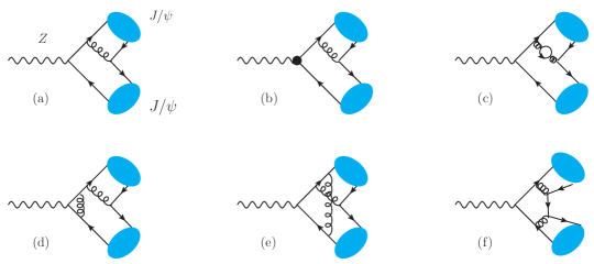
Figure 1: Representative QCD Feynman diagrams for $Z\to J/\psi(p_{1})+J/\psi(p_{2})$. $\textbf{a}(\mathcal{M}_{\alpha^{\frac{1}{2}}\alpha_{s}})$ is the tree-level diagram and $\textbf{b}-\textbf{f}(\mathcal{M}_{\alpha^{\frac{1}{2}}\alpha^{2}_{s}})$ are the NLO QCD corrections to a. Diagram b specifically represents the counter-term diagram.

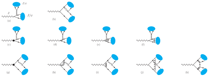
Figure 2: Representative QED Feynman diagrams for $Z\to J/\psi(p_{1})+J/\psi(p_{2})$. $\textbf{a},\textbf{b}(\mathcal{M}_{\alpha^{\frac{3}{2}}})$ are the tree-level diagram and $\textbf{c}-\textbf{k}(\mathcal{M}_{\alpha^{\frac{3}{2}}\alpha_{s}})$ are the NLO QCD corrections to $\textbf{a},\textbf{b}$. Diagrams c and g specifically represent the counter-term diagram.

The representative Feynman diagrams of $\mathcal{M}_{\alpha^{\frac{1}{2}}\alpha_{s}}$, $\mathcal{M}_{\alpha^{\frac{1}{2}}\alpha^{2}_{s}}$, $\mathcal{M}_{\alpha^{\frac{3}{2}}}$, and $\mathcal{M}_{\alpha^{\frac{3}{2}}\alpha_{s}}$ are displayed in figures 1 and 2. Figure 1(a) ($\alpha^{\frac{1}{2}}\alpha_{s}$ order) depicts the QCD tree-level diagram (4 diagrams), while figures 1(b-f) illustrate the corresponding NLO QCD corrections (56 one-loop diagrams and 20 counter-term diagrams). Figure 2(a,b) ($\alpha^{\frac{3}{2}}$ order) represent the tree-level diagrams for QED (8 diagrams), and figures 2(c-k) show the higher-order corrections in $\alpha_{s}$ (52 one-loop diagrams and 32 counter-term diagrams).

2.2 The decay width

The decay width in equation (6) can generally be written as

$$\Gamma^{\textrm{(0,1)}}_{i}=\frac{\kappa}{2m_{Z}}\frac{1}{2!N_{s}}\times\zeta_{i}\times\mathcal{C}^{(0,1)}_{i},~{}i=1,2,3,$$ (8)

with

$$\kappa = \frac{\sqrt{m^{2}_{Z}-16m^{2}_{c}}}{8\pi m_{Z}},$$

$$\zeta_{i} = \frac{\pi|R_{1S}(0)|^{4}}{256m_{c}^{6}\sin^{2}\theta_{\textrm{w}}\cos^{2}\theta_{\textrm{w}}}e^{2(i-1)}_{c}\alpha^{i}\alpha^{3-i}_{s},$$ (9)

where $N_{s}=3$ and $e_{c}=2/3$. The wave function at the origin, denoted as $|R_{1S}(0)|$, can be expressed in terms of NRQCD LDMEs by utilizing the following formulae

$$\langle\mathcal{O}^{J/\psi}(^{3}S_{1}^{1})\rangle=\frac{1}{4\pi}|R_{1S}(0)|^{2}.$$ (10)

2.2.1 LO

The LO processes depicted in figures 1(a) and 2(a,b) are free of divergence, enabling us to straightforwardly determine the coefficients of $\mathcal{C}^{(0)}_{i}$,

$$\mathcal{C}^{(0)}_{1} = \frac{65536m_{c}^{2}(r^{2}-10r+24)}{9r^{4}},$$

$$\mathcal{C}^{(0)}_{2} = \frac{16384m_{c}^{2}(3r+2)(r^{2}-10r+24)}{3r^{4}},$$

$$\mathcal{C}^{(0)}_{3} = \frac{1024m_{c}^{2}(3r+2)^{2}(r^{2}-10r+24)}{r^{4}},$$ (11)

where

$$r\equiv\frac{m^{2}_{Z}}{4m_{c}^{2}}.$$ (12)

2.2.2 NLO

Due to the color conservation, the NLO corrections to $Z\to J/\psi+J/\psi$ do not involve the real correction processes. We utilize the dimensional regularization with $D=4-2\epsilon$ to isolate the ultraviolet (UV) and infrared (IR) divergences. The on-shell mass (OS) scheme is employed to set the renormalization constants for the $c$-quark mass ($Z_{m}$) and heavy-quark field ($Z_{2}$); the minimal-subtraction ($\overline{MS}$) scheme is adopted for the QCD-gauge coupling ($Z_{g}$) and the gluon field $Z_{3}$. The renormalization constants are taken as

$$\delta Z_{m}^{OS} = -3C_{F}\frac{\alpha_{s}}{4\pi}N_{\epsilon}\left[\frac{1}{\epsilon_{\textrm{UV}}}+\frac{4}{3}+2\textrm{ln}{2}\right],$$

$$\delta Z_{2}^{OS} = -C_{F}\frac{\alpha_{s}}{4\pi}N_{\epsilon}\left[\frac{1}{\epsilon_{\textrm{UV}}}+\frac{2}{\epsilon_{\textrm{IR}}}+4+6\textrm{ln}{2}\right],$$

$$\delta Z_{3}^{\overline{MS}} = \frac{\alpha_{s}}{4\pi}(\beta_{0}-2C_{A})N_{\epsilon}\left[\frac{1}{\epsilon_{\textrm{UV}}}+\textrm{ln}\frac{4m_{c}^{2}}{\mu_{r}^{2}}\right],$$

$$\delta Z_{g}^{\overline{MS}} = -\frac{\beta_{0}}{2}\frac{\alpha_{s}}{4\pi}N_{\epsilon}\left[\frac{1}{\epsilon_{\textrm{UV}}}+\textrm{ln}\frac{4m_{c}^{2}}{\mu_{r}^{2}}\right],$$ (13)

where $N_{\epsilon}=\frac{1}{\Gamma[1-\epsilon]}\left(\frac{4\pi\mu_{r}^{2}}{4m_{c}^{2}}\right)^{\epsilon}$ is an overall factor, $\gamma_{E}$ is the Euler’s constant, and $\beta_{0}=\frac{11}{3}C_{A}-\frac{4}{3}T_{F}n_{f}$ is the one-loop coefficient of the $\beta$ function. $n_{f}(=n_{L}+n_{H})$ represents the number of the active-quark flavors; $n_{L}(=3)$ and $n_{H}(=1)$ denote the number of the light- and heavy-quark flavors, respectively. In ${\rm SU}(3)$, the color factors are given by $T_{F}=\frac{1}{2}$, $C_{F}=\frac{4}{3}$, and $C_{A}=3$.

With the inclusion of the QCD corrections, we acquire the coefficients of $\mathcal{C}^{(1)}_{i}$, which can be expressed in a general form

$$\mathcal{C}^{(1)}_{i}+\mathcal{C}^{(0)}_{i}=\mathcal{C}^{(0)}_{i}\left[1+\frac{\alpha_{s}}{\pi}\left(\xi_{i}\beta_{0}\textrm{ln}\frac{\mu_{r}^{2}}{4m_{c}^{2}}+a_{i}n_{L}+b_{i}n_{H}+c_{i}\right)\right],$$ (14)

where $\xi_{1}=\frac{1}{2}$, $\xi_{2}=\frac{1}{4}$, and $\xi_{3}=0$. The coefficients $a_{i}$, $b_{i}$, and $c_{i}$ are dependent solely on the variables of $r$ and $m_{c}$. One can find their fully-analytical expressions in Appendix LABEL:abc1-20. We in the following summarize the numerical values assigned to the coefficients of $a_{i}$, $b_{i}$, and $c_{i}$, corresponding to $m_{c}=1.5\pm 0.1$ GeV which is often adopted in charmonium-involved processes.

For $m_{c}=1.4$ GeV,

$$a_{1}=1.3045,~{}~{}b_{1}=1.3026,~{}~{}c_{1}=45.780;$$

$$a_{2}=0.6523,~{}~{}b_{2}=0.6513,~{}~{}c_{2}=20.527;$$

$$a_{3}=0,~{}~{}b_{3}=0,~{}~{}c_{3}=-4.7254.$$ (15)

For $m_{c}=1.5$ GeV,

$$a_{1}=1.2586,~{}~{}b_{1}=1.2564,~{}~{}c_{1}=43.832;$$

$$a_{2}=0.6293,~{}~{}b_{2}=0.6282,~{}~{}c_{2}=19.478;$$

$$a_{3}=0,~{}~{}b_{3}=0,~{}~{}c_{3}=-4.8767.$$ (16)

For $m_{c}=1.6$ GeV,

$$a_{1}=1.2155,~{}~{}b_{1}=1.2130,~{}~{}c_{1}=42.063;$$

$$a_{2}=0.6078,~{}~{}b_{2}=0.6065,~{}~{}c_{2}=18.523;$$

$$a_{3}=0,~{}~{}b_{3}=0,~{}~{}c_{3}=-5.0183.$$ (17)

We utilize FeynArts Hahn:2000kx to generate all the necessary Feynman diagrams and corresponding analytical amplitudes. Following this, we apply the package FeynCalc Mertig:1990an to handle the traces of the $\gamma$ and color matrices, which transforms the hard scattering amplitudes into expressions with loop integrals. When calculating the $D$-dimensional $\gamma$ traces that incorporate a single $\gamma_{5}$ matrix and involve UV and/or IR divergences, following the scheme outlined in refs. Korner:1991sx ; z decay 4 ; z decay 22 , we choose the same starting point ($Z$-vertex) to write down the amplitudes without implementation of cyclicity. Afterward, we employ our self-written Mathematica codes that include implementations of Apart Feng:2012iq and FIRE Smirnov:2008iw to reduce these loop integrals to a set of irreducible Master Integrals, whose fully-analytical expressions can be found in Appendix 22-32. As a cross check, we simultaneously adopt the package LoopTools Hahn:1998yk to numerically evaluate these Master Integrals, acquiring the same numerical results.

We have refined our calculating framework used in the heavy-quarkonium production in $e^{+}e^{-}$ annihilation Sun:2018rgx ; Sun:2021tma or $Z$-boson decay z decay 31 ; z decay 33 ; z decay 34 ; z decay 35 to deal with the calculations within the context. The two processes bear a resemblance of NLO diagrams and $\gamma_{5}$-trace structure to $Z\to J/\psi+J/\psi$. In addition, we have calculated the process of $Z\to J/\psi+\eta_{c}$ and obtained the same $K$ factor as in the $e^{+}e^{-}$ annihilation.

3 Phenomenological results

In the calculations, we choose $m_{c}=m_{J/\psi}/2=1.5\pm 0.1$ GeV, $m_{Z}=91.1876$ GeV, $\alpha=1/128$ z decay 4 , and employ the two-loop $\alpha_{s}$ running coupling constant. The wave function at the origin is configured as $|R_{1S}(0)|^{2}=0.81~{}\textrm{GeV}^{3}$ Eichten:1995ch .

Table 1: Decay widths (in unit: $10^{-12}$ GeV) of $Z\to J/\psi+J/\psi$ with $m_{c}=1.5$ GeV. “$\Gamma^{\textrm{LO}}_{\textrm{total}}$" incorporates the individual contributions of $\Gamma^{(0)}_{1}$, $\Gamma^{(0)}_{2}$, and $\Gamma^{(0)}_{3}$, while “$\Gamma^{\textrm{NLO}}_{\textrm{total}}$" refers to the combined sum of the contributions of $\Gamma^{(0,1)}_{1,2,3}$.

$\mu_{r}$	$\Gamma^{(0)}_{1}$	$\Gamma^{(1)}_{1}$	$\Gamma^{(0)}_{2}$	$\Gamma^{(1)}_{2}$	$\Gamma^{(0)}_{3}$	$\Gamma^{(1)}_{3}$	$\Gamma^{\textrm{LO}}_{\textrm{total}}$	$\Gamma^{\textrm{NLO}}_{\textrm{total}}$
$2m_{c}$	$1.458$	$5.850$	$40.71$	$73.43$	$284.2$	$-115.2$	$326.4$	$290.4$
$m_{Z}/2$	$0.387$	$1.173$	$20.98$	$29.59$	$284.2$	$-59.38$	$305.6$	$277.0$
$m_{Z}$	$0.309$	$0.906$	$18.76$	$25.71$	$284.2$	$-53.10$	$303.3$	$276.8$

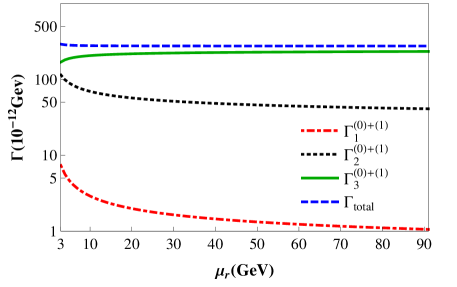
Figure 3: Decay widths of $Z\to J/\psi+J/\psi$ as a function of the renormalization scale with $m_{c}=1.5$ GeV. “$\Gamma_{\textrm{total}}$" refers to the combined sum of the contributions of $\Gamma^{(0,1)}_{1,2,3}$.

Table 1 summarizes our predictions of the decay width of $Z\to J/\psi+J/\psi$. Inspecting the data, one can find

• At the LO accuracy in $\alpha_{s}$, the pure QCD prediction, known as $\Gamma^{(0)}_{1}$, is around $10^{-12}$. However, when the QED diagrams are taken into account, the inclusion of $\Gamma^{(0)}_{2,3}$ significantly enhances the QCD results, resulting in an increase of approximately 2-3 orders of magnitude. The remarkable contribution of the QED diagram can mainly be attributed to the kinematic enhancement arising from the single-photon-fragmentation structure in figure 2(a), which compensates sufficiently for the $\alpha$ suppression and then dominates over figure 1(a).

• After incorporating the QCD corrections, the QCD results would experience a significant amplification of approximately 4-5 times, as demonstrated by the ratio of $\left(\Gamma^{(0)}_{1}+\Gamma^{(1)}_{1}\right)\big{/}\Gamma^{(0)}_{1}$. Of the NLO contributions, the fermion-loop diagram, i.e. figure 1(c), accounts for approximately $20\%$. However, including the higher-order terms in $\alpha_{s}$ would considerably diminish the pure QED results, e.g., $\left(\Gamma^{(0)}_{3}+\Gamma^{(1)}_{3}\right)\big{/}\Gamma^{(0)}_{3}\sim 60-80\%$. As a result of the combined influence of enhancement and reduction effects, the QCD corrections will lead to a increase of about 2.5-3 times in the interference terms, as can be verified by referring to $\left(\Gamma^{(0)}_{2}+\Gamma^{(1)}_{2}\right)\big{/}\Gamma^{(0)}_{2}$. It is worth noting that the rise in $\Gamma^{(1)}_{3}$ towards higher renormalization scale ($\mu_{r}$) would compensate for the declines in $\Gamma^{(1)}_{1}$ and $\Gamma^{(1)}_{2}$, ultimately causing a steady $\mu_{r}$ dependence of the total NLO prediction, as depicted in figure 3.

Table 2: Comparisons of our predicted branching ratio with experiment. “$\mathcal{B}_{\textrm{theo}}$" stands for the theoretical results, comprised of the contributions of $\Gamma^{(0,1)}_{1,2,3}$. The central value corresponds to $\mu_{r}=m_{Z}/2$ and $m_{c}=1.5$ GeV. The uncertainties in the first column are due to the variation of $m_{c}$ within the range of $1.4$ to $1.6$ GeV, while the second column of uncertainties are caused by varying $\mu_{r}$ from $2m_{c}$ to $m_{Z}$.

$\mathcal{B}_{\textrm{exp}}$ CMS:2022fsq	${\mathcal{B}}_{\textrm{theo}}$
$<1.4\times 10^{-6}$	$(1.110^{+0.334+0.054}_{-0.241-0.001})\times 10^{-10}$

At last, we validate our predictions with experimentation. The results, as presented in table 2, indicate that the calculated $\mathcal{B}_{Z\to J/\psi+J/\psi}$ noticeably undershoot the upper limit established by the CMS Collaboration. The variation of $m_{c}$ by 0.1 GeV around 1.5 GeV would lead to a prediction alteration by $20-30\%$. Conversely, the deviation of $\mu_{r}$ from $2m_{c}$ to $m_{Z}$ around $m_{Z}/2$ just has a slight impact on the predictions. The upper experimental bound instead of precise measurement implies the failure to detect this branching above the existing $Z$ production rate at the currently running LHC. Hopefully, the future CEPC experiment will have the capability to provide a detailed measurement of this decay channel.

4 Summary

In order to provide deeper insights into $Z\to J/\psi+J/\psi$, we in this paper conducted a NLO study of this process using the NRQCD framework. Our LO results indicate that the contributions from QED diagrams dominate over those from QCD diagrams. The QCD corrections have a substantial amplifying effect on the QCD results, while simultaneously diminishing the QED results. By considering both the QCD and QED contributions, we estimated the branching ratio to be $\mathcal{B}_{Z\to J/\psi+J/\psi}=(1.110^{+0.334+0.054}_{-0.241-0.001})\times 10^{-10}$, which exhibits a rather steady renormalization-scale dependence. This prediction falls significantly below the upper limits set by the CMS Collaboration.

Appendix A Analytical NLO expressions

In this section, we list the analytical expressions of the coefficients $a_{i}$, $b_{i}$, and $c_{i}$ in equation (14), which are written as a superposition of the Master Integrals $\mathcal{I}$.

A.1 NLO coefficients

$$a_{1} = \frac{-3\mathcal{I}^{(2)}_{2}+1-6\ln(2m_{c})}{9},$$

$$b_{1} = \frac{6\mathcal{I}_{1}-3m_{c}^{2}(r+2)\mathcal{I}^{(3)}_{2}+m_{c}^{2}\left[r-6-6r\ln(2m_{c})\right]}{9m_{c}^{2}r},$$

$$c_{1} = \frac{76r^{4}-151r^{3}+228r^{2}+216r+24}{3m_{c}^{2}r(2r+1)(r^{2}-10r+24)}\mathcal{I}_{1}+\frac{-496r^{4}+109r^{3}+1000r^{2}+644r+120}{6r^{4}-57r^{3}+114r^{2}+72r}\mathcal{I}^{(1)}_{2}$$

$$+\frac{179r^{2}-469r+348}{3r^{2}-30r+72}\mathcal{I}^{(2)}_{2}+\frac{-5r^{2}-68r+304}{18(r^{2}-10r+24)}\mathcal{I}^{(3)}_{2}+\frac{2(95r^{2}+131r-412)}{9(r^{2}-10r+24)}I^{(4)}_{2}$$

$$+\frac{4m_{c}^{2}r(r^{2}-5r+20)}{3(r^{2}-10r+24)}\mathcal{I}^{(1)}_{3}-\frac{m_{c}^{2}(113r^{3}+160r^{2}-712r+240)}{24(r^{2}-10r+24)}\mathcal{I}^{(2)}_{3}+\frac{m_{c}^{2}(7r^{3}-52r^{2}+50r+48)}{3(r^{2}-10r+24)}\mathcal{I}^{(3)}_{3}$$

$$+\frac{m_{c}^{2}(-303r^{3}+144r^{2}+488r-144)}{24(r^{2}-10r+24)}\mathcal{I}^{(4)}_{3}+\frac{2m_{c}^{2}(11r^{3}+66r^{2}-198r+120)}{3(r^{2}-10r+24)}\mathcal{I}^{(5)}_{3}$$

$$+\frac{2m_{c}^{2}(r^{3}-6r^{2}+24r-48)}{3(r^{2}-10r+24)}\mathcal{I}^{(6)}_{3}-\frac{179r^{3}-3146r^{2}+6936r+1584}{18r(r^{2}-10r+24)}+(\frac{4}{r}+21)\ln(m_{c})+11\ln(2).$$

$$a_{2} = \frac{-3\mathcal{I}^{(2)}_{2}+1-6\ln(2m_{c})}{18},$$

$$b_{2} = \frac{6\mathcal{I}_{1}-3m_{c}^{2}(r+2)\mathcal{I}^{(3)}_{2}+m_{c}^{2}\left[r-6-6r\ln(2m_{c})\right]}{18m_{c}^{2}r},$$

$$c_{2} = \frac{177r^{5}-484r^{4}+658r^{3}+792r^{2}+720r+264}{3m_{c}^{2}r(2r+1)(3r+2)(r^{2}-10r+24)}\mathcal{I}_{1}$$ (19)

$$+\frac{-1500r^{5}-2761r^{4}+5650r^{3}+7264r^{2}+2000r+48}{6r(6r^{4}-53r^{3}+76r^{2}+148r+48)}\mathcal{I}^{(1)}_{2}+\frac{537r^{3}-769r^{2}-790r+1464}{6(3r+2)(r^{2}-10r+24)}\mathcal{I}^{(2)}_{2}$$

$$-\frac{15r^{3}+134r^{2}-1864r+4256}{36(3r+2)(r^{2}-10r+24)}\mathcal{I}^{(3)}_{2}+\frac{267r^{3}+1655r^{2}-2566r-280}{9(3r+2)(r^{2}-10r+24)}I^{(4)}_{2}$$

$$+\frac{2m_{c}^{2}r(3r^{3}-56r^{2}+184r-64)}{3(3r+2)(r^{2}-10r+24)}\mathcal{I}^{(1)}_{3}-\frac{m_{c}^{2}(339r^{4}+1058r^{3}-3512r^{2}+3776r-3360)}{48(3r+2)(r^{2}-10r+24)}\mathcal{I}^{(2)}_{3}$$

$$+\frac{m_{c}^{2}(21r^{4}-110r^{3}-238r^{2}+1028r-672)}{6(3r+2)(r^{2}-10r+24)}\mathcal{I}^{(3)}_{3}-\frac{m_{c}^{2}(909r^{4}+654r^{3}-2904r^{2}+1504r-2016)}{48(3r+2)(r^{2}-10r+24)}\mathcal{I}^{(4)}_{3}$$

$$+\frac{m_{c}^{2}(21r^{4}+506r^{3}-1050r^{2}+252r+48)}{3(3r+2)(r^{2}-10r+24)}\mathcal{I}^{(5)}_{3}+\frac{m_{c}^{2}(3r^{4}-32r^{3}+156r^{2}-480r+672)}{3(3r+2)(r^{2}-10r+24)}\mathcal{I}^{(6)}_{3}$$

$$-\frac{1311r^{4}-17284r^{3}+28324r^{2}+39984r+3744}{36r(3r+2)(r^{2}-10r+24)}+(\frac{4}{r}+\frac{31}{2})\ln(m_{c})+\frac{11\ln(2)}{2}.$$

$$a_{3} = b_{3}=0,$$

$$c_{3} = \frac{126r^{5}-667r^{4}+934r^{3}+480r^{2}+936r+480}{3m_{c}^{2}r(2r+1)(3r+2)(r^{2}-10r+24)}\mathcal{I}_{1}-\frac{4(3r^{5}+524r^{4}-608r^{3}-833r^{2}-88r+48)}{3r(2r+1)(3r+2)(r^{2}-10r+24)}\mathcal{I}^{(1)}_{2}$$ (20)

$$+\frac{8(35r^{2}-112r+96)}{3(3r+2)(r^{2}-10r+24)}\mathcal{I}^{(2)}_{2}+\frac{8(5r^{2}+68r-304)}{9(3r+2)(r^{2}-10r+24)}\mathcal{I}^{(3)}_{2}-\frac{4(9r^{3}-536r^{2}+796r-272)}{9(3r+2)(r^{2}-10r+24)}I^{(4)}_{2}$$

$$-\frac{4m_{c}^{2}r(43r^{2}-134r+104)}{3(3r+2)(r^{2}-10r+24)}\mathcal{I}^{(1)}_{3}+\frac{4m_{c}^{2}(-11r^{3}+53r^{2}-140r+120)}{3(3r+2)(r^{2}-10r+24)}\mathcal{I}^{(2)}_{3}$$

$$+\frac{4m_{c}^{2}(8r^{3}-71r^{2}+196r-192)}{3(3r+2)(r^{2}-10r+24)}\mathcal{I}^{(3)}_{3}-\frac{4m_{c}^{2}(15r^{3}-36r^{2}+64r-72)}{3(3r+2)(r^{2}-10r+24)}\mathcal{I}^{(4)}_{3}$$

$$-\frac{4m_{c}^{2}(6r^{4}-143r^{3}+294r^{2}-144r+96)}{3(3r+2)(r^{2}-10r+24)}\mathcal{I}^{(5)}_{3}-\frac{32m_{c}^{2}(r^{3}-6r^{2}+24r-48)}{3(3r+2)(r^{2}-10r+24)}\mathcal{I}^{(6)}_{3}$$

$$-\frac{387r^{4}-4102r^{3}+6904r^{2}+10680r+288}{9r(3r+2)(r^{2}-10r+24)}+(\frac{4}{r}+10)\ln(m_{c}).$$

A.2 Master Integrals

Here we just present the finite ($\epsilon^{0}$-order) terms of the Master Integrals in LABEL:abc1-20. For brevity, we define

$$a=\sqrt{r},~{}b=\sqrt{r-1},~{}c=\sqrt{r-4},~{}d=2r+1,$$

$$f=r+ac-4,~{}g=r-ac-4,~{}h=rg+2ac,$$

$$j=rf-2ac,~{}j_{1}=(r-4)ab,~{}j_{2}=(2-r)bc.$$ (21)

There is only one 1-point scalar integral

$$\mathcal{I}_{1} = \frac{\lambda}{\mu_{r}^{4-D}}\int{\frac{d^{D}k}{k^{2}-m_{c}^{2}}}=m_{c}^{2}\left[1-2\ln(m_{c})\right],$$ (22)

where $k$ denotes the loop momentum, $\lambda=\frac{\mu_{r}^{4-D}}{i\pi^{\frac{D}{2}}\gamma_{\Gamma}}$ with $\gamma_{\Gamma}=\frac{\Gamma^{2}(1-\epsilon)\Gamma(1+\epsilon)}{\Gamma(1-2\epsilon)}$.
There are four 2-point scalar integrals,

$$\mathcal{I}^{(1)}_{2} = \frac{\lambda}{\mu_{r}^{4-D}}\int{\frac{d^{D}k}{k^{2}[(k+\frac{2p_{1}+p_{2}}{2})^{2}-m_{c}^{2}]}}=2-2\ln{(m_{c})}-\frac{2r}{d}\left[\ln{(2r)}-i\pi\right],$$

$$\mathcal{I}^{(2)}_{2} = \frac{\lambda}{\mu_{r}^{4-D}}\int{\frac{d^{D}k}{k^{2}(k-\frac{p_{1}+p_{2}}{2})^{2}}}=2-\ln{({m_{c}}^{2}r)}+i\pi.$$ (24)

$$\mathcal{I}^{(3)}_{2} = \frac{\lambda}{\mu_{r}^{4-D}}\int\frac{d^{D}k}{(k^{2}-m_{c}^{2})[(k+\frac{p_{1}+p_{2}}{2})^{2}-m_{c}^{2}]}=\frac{c}{a}\left[\ln{\left(\frac{4r}{(f+4)^{2}}\right)}+i\pi\right]+2\left[1-\ln{(m_{c})}\right],$$

$$\mathcal{I}^{(4)}_{2} = \frac{\lambda}{\mu_{r}^{4-D}}\int\frac{d^{D}k}{(k^{2}-m_{c}^{2})[(k+p_{1}+p_{2})^{2}-m_{c}^{2}]}=\frac{b}{a}\left[\ln{(-2ab+d-2)}+i\pi\right]+2\left[1-\ln{(m_{c})}\right].$$

There are six 3-point scalar integrals,

$$\mathcal{I}^{(1)}_{3} = \frac{\lambda}{\mu_{r}^{4-D}}\int\frac{d^{D}k}{k^{2}[(k+\frac{p_{2}}{2})^{2}-m_{c}^{2}][(k+\frac{2p_{1}+p_{2}}{2})^{2}-m_{c}^{2}]}$$ (27)

$$=\frac{1}{2acm_{c}^{2}}\left\{{\ln(2)\ln\left(\frac{(3(g+4)+h)^{2}}{d(g+h+4)^{2}}\right)+\left[\ln(r)-i\pi\right]\ln\left(\frac{d}{(g+3)^{2}}\right)+4\textrm{Li}_{2}\left(\frac{c}{a}\right)+\textrm{Li}_{2}\left(-\frac{2(ac+j)}{d}\right)}\right.$$

$$\left.{-\textrm{Li}_{2}\left(\frac{c^{2}}{ac-h}\right)-\textrm{Li}_{2}\left(-\frac{c+ag}{a}\right)-2\textrm{Li}_{2}\left(-\frac{c}{a}\right)}\right\},$$

$$\mathcal{I}^{(2)}_{3} = \frac{\lambda}{\mu_{r}^{4-D}}\int\frac{d^{D}k}{k^{2}[(k-\frac{p_{2}}{2})^{2}-m_{c}^{2}](k+\frac{p_{1}+p_{2}}{2})^{2}}$$ (28)

$$=\frac{1}{acm_{c}^{2}}\left\{{\ln(2)\ln\left(\frac{d(f+4)^{2}}{(3r-ac)^{2}}\right)+\left[\ln(r)-i\pi)\right]\ln\left(\frac{4dr}{(3r-ac)^{2}}\right)+\textrm{Li}_{2}\left(-\frac{2(ac+j)}{d}\right)+2\textrm{Li}_{2}\left(\frac{c}{a}\right)}\right.$$

$$\left.{+\textrm{Li}_{2}\left(-\frac{g}{2}\right)-\textrm{Li}_{2}\left(-\frac{f}{2}\right)-\textrm{Li}_{2}\left(\frac{c^{2}}{ac-h}\right)-\textrm{Li}_{2}\left(-\frac{c+ag}{a}\right)}\right\},$$

$$\mathcal{I}^{(3)}_{3} = \frac{\lambda}{\mu_{r}^{4-D}}\int\frac{d^{D}k}{k^{2}[(k+\frac{p_{1}}{2})^{2}-m_{c}^{2}](k+\frac{p_{1}+p_{2}}{2})^{2}}$$

$$=\frac{1}{acm_{c}^{2}}\left\{\left[\ln(r)-i\pi\right]\ln\left(\frac{(f+4)^{2}}{4r}\right)+2\textrm{Li}_{2}\left(\frac{c}{a}\right)-2\textrm{Li}_{2}\left(-\frac{c}{a}\right)-\textrm{Li}_{2}\left(-\frac{g}{2}\right)+\textrm{Li}_{2}\left(-\frac{f}{2}\right)\right\},$$

$$\mathcal{I}^{(4)}_{3} = \frac{\lambda}{\mu_{r}^{4-D}}\int\frac{d^{D}k}{k^{2}[(k+\frac{2p_{1}+p_{2}}{2})^{2}-m_{c}^{2}](k+\frac{p_{1}+p_{2}}{2})^{2}}$$ (30)

$$=\frac{1}{acm_{c}^{2}}\left\{{\ln(2)\ln\left(\frac{d}{(g+3)^{2}}\right)+\left[\ln(r)-i\pi)\right]\ln\left(\frac{g+6}{2g+6}\right)+\textrm{Li}_{2}\left(-\frac{g}{2}\right)-\textrm{Li}_{2}\left(-\frac{f}{2}\right)-2\textrm{Li}_{2}\left(-\frac{c}{a}\right)}\right.$$

$$\left.{-\textrm{Li}_{2}\left(\frac{2ac-2h}{d}\right)+\textrm{Li}_{2}\left(\frac{h-ac}{dr}\right)+\textrm{Li}_{2}\left(\frac{c}{a}-f\right)}\right\},$$

$$\mathcal{I}^{(5)}_{3} = \frac{\lambda}{\mu_{r}^{4-D}}\int\frac{d^{D}k}{k^{2}[(k-\frac{p_{1}}{2})^{2}-m_{c}^{2}][(k+\frac{p_{1}+2p_{2}}{2})^{2}-m_{c}^{2}]}$$

$$=\frac{1}{2acm_{c}^{2}}\left\{{\left[\ln\left(\frac{(r-ab)^{2}}{r}\right)+i\pi\right]\ln\left(\frac{br(2b-3c)+j-j_{1}}{br(2b+3c)+j+j_{1}}\right)+\left[\ln(2r)-i\pi\right]\ln\left(\frac{(g+3)^{2}}{d}\right)}\right.$$

$$\left.{{-\textrm{Li}_{2}\left(-\frac{2(ac+j)}{d}\right)-\textrm{Li}_{2}\left(\frac{c^{2}-h+j_{1}+j_{2}}{r}\right)-\textrm{Li}_{2}\left(-\frac{-c^{2}+h+j_{1}+j_{2}}{r}\right)+\textrm{Li}_{2}\left(\frac{c^{2}-j+j_{1}-j_{2}}{r}\right)}}\right.$$

$$\left.{-2\textrm{Li}_{2}\left(-\frac{c}{a}\right)+\textrm{Li}_{2}\left(\frac{c^{2}-j-j_{1}+j_{2}}{r}\right)+{\textrm{Li}_{2}\left(\frac{c^{2}}{ac-h}\right)+\textrm{Li}_{2}\left(-\frac{c+ag}{a}\right)}}\right\},$$

$$\mathcal{I}^{(6)}_{3} = \frac{\lambda}{\mu_{r}^{4-D}}\int\frac{d^{D}k}{k^{2}[(k+\frac{p_{2}}{2})^{2}-m_{c}^{2}][(k+\frac{p_{1}+2p_{2}}{2})^{2}-m_{c}^{2}]}$$ (32)

$$=\frac{1}{acm_{c}^{2}}\left\{{\ln(2)\ln\left(\frac{(f+4)^{4}\left(3(2r-ac)+h\right)}{4(g+6)\left(4(r-ac)+h\right)}\right)+\ln(r)\ln\left(\frac{dr}{(d+f+3)^{2}}\right)-i\pi\ln\left(\frac{16d}{(g+6)^{2}r}\right)}\right.$$

$$\left.{+\textrm{Li}_{2}\left(-\frac{g}{8}\right)+\textrm{Li}_{2}\left(-\frac{4ac+j}{2d}\right)-\textrm{Li}_{2}\left(\frac{4ac-h}{4r}\right)+2\textrm{Li}_{2}\left(\frac{c}{2a}\right)+\textrm{Li}_{2}\left(\frac{f}{2r}\right)-\textrm{Li}_{2}\left(-\frac{f}{8}\right)-\textrm{Li}_{2}\left(\frac{g}{2r}\right)}\right.$$

$$\left.{-\textrm{Li}_{2}\left(\frac{c^{2}}{4ac-h}\right)}\right\}.$$

- (1) A. M. Sirunyan et al. [CMS], Search for Higgs and Z boson decays to J/ or Y pairs in the four-muon final state in proton-proton collisions at s=13TeV, Phys. Lett. B797 (2019), 134811, [arXiv:1905.10408].
- (2) A. Tumasyan et al. [CMS], Search for Higgs boson decays into Z and J/ and for Higgs and Z boson decays into J/ or Y pairs in pp collisions at s=13 TeV, Phys. Lett. 842 (2023), 137534, [arXiv:2206.03525].
- (3) A. K. Likhoded and A. V. Luchinsky, Double Charmonia Production in Exclusive Boson Decays, Mod. Phys. Lett. A33 (2018) no.14, 1850078, [arXiv:1712.03108].
- (4) D. N. Gao and X. Gong, Note on rare Z-boson decays to double heavy quarkonia*, Chin. Phys. C47 (2023) no.4, 043106, [arXiv:2208.12652].
- (5) Y. J. Zhang, Y. j. Gao and K. T. Chao, Next-to-leading order QCD correction to e+ e- —> J / psi + eta(c) at s**(1/2) = 10.6-GeV, Phys. Rev. Lett. 96 (2006) 092001, [hep-ph/0506076].
- (6) B. Gong and J. X. Wang, QCD corrections to plus production in annihilation at = 10.6-GeV, Phys. Rev. D77 (2008) 054028, [arXiv:0712.4220].
- (7) Y. J. Zhang, Y. Q. Ma and K. T. Chao, Factorization and NLO QCD correction in at B Factories, Phys. Rev. D78 (2008) 054006, [arXiv:0802.3655].
- (8) N. Brambilla et al., Heavy Quarkonium: Progress, Puzzles, and Opportunities, Eur. Phys. J. C71 (2011) 1534, [arXiv:1010.5827].
- (9) H. R. Dong, F. Feng and Y. Jia, corrections to production at factories, JHEP 1110 (2011) 141, Erratum: [JHEP 1302 (2013) 089], [arXiv:1107.4351].
- (10) Z. Sun, X. G. Wu, Y. Ma and S. J. Brodsky, Exclusive production of at the factories Belle and Babar using the principle of maximum conformality, Phys. Rev. D98 (2018) no.9, 094001, [arXiv:1807.04503].
- (11) Z. Sun, Next-to-leading-order study of angular distributions in at GeV, JHEP 09 (2021), 073, [arXiv:2107.02047].
- (12) B. Guberina, J. H. Kuhn, R. D. Peccei and R. Ruckl, Rare Decays of the Z0, Nucl. Phys. B174 (1980) 317-334.
- (13) W. Y. Keung, Off Resonance Production of Heavy Vector Quarkonium States in Annihilation, Phys. Rev. D23 (1981) 2072.
- (14) V. D. Barger, K. m. Cheung and W. Y. Keung, Z BOSON DECAYS TO HEAVY QUARKONIUM, Phys. Rev. D41 (1990) 1541.
- (15) E. Braaten, K. m. Cheung and T. C. Yuan, Z0 decay into charmonium via charm quark fragmentation, Phys. Rev. D48 (1993) 4230-4235, [hep-ph/9302307].
- (16) S. Fleming, Electromagnetic production of quarkonium in Z0 decay, Phys. Rev. D48 (1993) R1914-R1916, [hep-ph/9304270].
- (17) G. Alexander et al. [OPAL], Prompt J / psi production in hadronic Z0 decays, Phys. Lett. B384 (1996) 343-352.
- (18) P. Abreu et al. [DELPHI], Search for promptly produced heavy quarkonium states in hadronic Z decays, Z. Phys. C69 (1996) 575-584.
- (19) K. m. Cheung, W. Y. Keung and T. C. Yuan, Color octet quarkonium production at the pole, Phys. Rev. Lett. 76 (1996) 877-880, [hep-ph/9509308].
- (20) P. L. Cho, Prompt upsilon and psi production at LEP, Phys. Lett. B368 (1996) 171-178, [hep-ph/9509355].
- (21) S. Baek, P. Ko, J. Lee and H. S. Song, Color octet heavy quarkonium productions in Z0 decays at LEP, Phys. Lett. B389 (1996) 609-615, [hep-ph/9607236].
- (22) P. Ernstrom, L. Lonnblad and M. Vanttinen, Evolution effects in fragmentation into charmonium, Z. Phys. C76 (1997) 515-521, [hep-ph/9612408].
- (23) E. M. Gregores, F. Halzen and O. J. P. Eboli, Prompt charmonium production in Z decays, Phys. Lett. B395 (1997) 113-117, [hep-ph/9607324].
- (24) C. f. Qiao, F. Yuan and K. T. Chao, A Crucial test for color octet production mechanism in decays, Phys. Rev. D55 (1997) 4001-4004, [hep-ph/9609284].
- (25) S. Baek, P. Ko, J. Lee and H. S. Song, Color octet mechanism and polarization at LEP, Phys. Rev. D55 (1997) 6839-6843, [hep-ph/9701208].
- (26) M. Acciarri et al. [L3], Inclusive , and chi() production in hadronic decays, Phys. Lett. B407 (1997) 351-360.
- (27) M. Acciarri et al. [L3], Heavy quarkonium production in decays, Phys. Lett. B453 (1999) 94-106.
- (28) C. G. Boyd, A. K. Leibovich and I. Z. Rothstein, J / psi production at LEP: Revisited and resummed, Phys. Rev. D59 (1999) 054016, [hep-ph/9810364].
- (29) M. Acciarri et al. [L3], Heavy quarkonium production in decays, Phys. Lett. B453 (1999) 94-106.
- (30) R. Li and J. X. Wang, The next-to-leading-order QCD correction to inclusive production in decay, Phys. Rev. D82 (2010) 054006, [arXiv:1007.2368].
- (31) L. C. Deng, X. G. Wu, Z. Yang, Z. Y. Fang and Q. L. Liao, Boson Decays to Meson and Its Uncertainties, Eur. Phys. J. C70 (2010) 113-124, [arXiv:1009.1453].
- (32) Z. Yang, X. G. Wu, L. C. Deng, J. W. Zhang and G. Chen, Production of the -Wave Excited -States through the Boson Decays, Eur. Phys. J.C71 (2011) 1563, [arXiv:1011.5961].
- (33) C. F. Qiao, L. P. Sun and R. L. Zhu, The NLO QCD Corrections to Meson Production in Decays, JHEP 08 (2011) 131, [arXiv:1104.5587].
- (34) T. C. Huang and F. Petriello, Rare exclusive decays of the Z-boson revisited, Phys. Rev. D92 (2015) 014007, [arXiv:1411.5924].
- (35) J. Jiang, L. B. Chen and C. F. Qiao, QCD NLO corrections to inclusive production in decays, Phys. Rev. D91 (2015) 034033, [arXiv:1501.00338].
- (36) Q. L. Liao, Y. Yu, Y. Deng, G. Y. Xie and G. C. Wang, Excited heavy quarkonium production via Z0 decays at a high luminosity collider, Phys. Rev. D91 (2015) 114030, [arXiv:1505.03275].
- (37) G. Aad et al. [ATLAS], Search for Higgs and Z Boson Decays to and with the ATLAS Detector, Phys. Rev. Lett. 114 (2015) 121801, [arXiv:1501.03276].
- (38) Y. Grossman, M. König and M. Neubert, Exclusive Radiative Decays of W and Z Bosons in QCD Factorization, JHEP 04 (2015) 101, [arXiv:1501.06569]
- (39) G. T. Bodwin, H. S. Chung, J. H. Ee and J. Lee, -boson decays to a vector quarkonium plus a photon, Phys. Rev. D97 (2018) 016009, [arXiv:1709.09320].
- (40) A. K. Likhoded and A. V. Luchinsky, Double Charmonia Production in Exclusive Boson Decays, Mod. Phys. Lett. A33 (2018) 1850078, [arXiv:1712.03108].
- (41) M. Aaboud et al. [ATLAS], Searches for exclusive Higgs and boson decays into , , and at TeV with the ATLAS detector, Phys. Lett. B786 134-155, [arXiv:1807.00802].
- (42) Z. Sun and H. F. Zhang, Next-to-leading-order QCD corrections to the decay of boson into , Phys. Rev. D99 (2019) 094009, [arXiv:1809.02426].
- (43) J. P. Lansberg, New Observables in Inclusive Production of Quarkonia, Phys. Rept. 889 (2020) 1, [arXiv:1903.09185].
- (44) A. M. Sirunyan et al. [CMS], Search for rare decays of Z and Higgs bosons to J and a photon in proton-proton collisions at 13 TeV, Eur. Phys. J. C79 (2019) 94, [arXiv:1810.10056].
- (45) Z. Sun, The studies on at the next-to-leading-order QCD accuracy, Eur. Phys. J. C80 (2020) 311, [arXiv:2002.03290].
- (46) Z. Sun and H. F. Zhang, Comprehensive studies of inclusive production in Z boson decay, JHEP 06 (2021), 152, [arXiv:2104.08711].
- (47) Z. Sun, X. Luo and Y. Z. Jiang, Impact of on the inclusive meson yield in Z-boson decay, Phys. Rev. D106 (2022) no.3, 034001, [arXiv:2112.00223].
- (48) X. C. Zheng, X. G. Wu, X. J. Zhan, H. Zhou and H. T. Li, Next-to-leading order QCD corrections to , Phys. Rev. D106 (2022) no.9, 094008, [arXiv:2205.03768].
- (49) W. L. Sang, D. S. Yang and Y. D. Zhang, Z boson radiative decays to a P-wave quarkonium at NNLO and LL accuracy, Phys. Rev. D106 (2022) no.9, 094023, [arXiv:2208.10118].
- (50) W. L. Sang, D. S. Yang and Y. D. Zhang, boson radiative decays to a -wave quarkonium at NNLO and NLL accuracy, [arXiv:2302.06439].
- (51) J. B. Guimarães da Costa et al. [CEPC Study Group], CEPC Conceptual Design Report: Volume 2 - Physics & Detector, [arXiv:1811.10545].
- (52) G. T. Bodwin, E. Braaten and G. P. Lepage, Rigorous QCD analysis of inclusive annihilation and production of heavy quarkonium, Phys. Rev. D51 (1995) 1125, Erratum: [Phys. Rev D55 (1997) 5853], [hep-ex/9407339].
- (53) A. Petrelli, M. Cacciari, M. Greco, F. Maltoni and M. L. Mangano, NLO production and decay of quarkonium, Nucl. Phys.B514 (1998), 245-309, [hep-ph/9707223].
- (54) T. Hahn, Generating Feynman diagrams and amplitudes with FeynArts 3, Comput. Phys. Commun. 140 (2001) 418-431, [hep-ph/0012260].
- (55) R. Mertig, M. Bohm and A. Denner, FEYN CALC: Computer algebraic calculation of Feynman amplitudes, Comput. Phys. Commun. 64 345-359.
- (56) J. G. Korner, D. Kreimer and K. Schilcher, A Practicable scheme in dimensional regularization, Z. Phys. C54 (1992), 503-512.
- (57) F. Feng, : A Generalized Mathematica Apart Function, Comput. Phys. Commun. 183 (2012) 2158-2164, [arXiv:1204.2314].
- (58) A. V. Smirnov, Algorithm FIRE – Feynman Integral REduction, JHEP 10 (2008) 107, [arXiv:0807.3243].
- (59) T. Hahn and M. Perez-Victoria, Automatized one loop calculations in four-dimensions and D-dimensions, Comput. Phys. Commun. 118 (1999) 153, [hep-ex/9807565].
- (60) E. J. Eichten and C. Quigg, Quarkonium wave functions at the origin, Phys. Rev. D52 (1995) 1726-1728, [hep-ph/9503356].