Solution for cosmological observables in the Starobinsky model of inflation

Abstract

This paper focuses on the Starobinsky model of inflation in the Einstein frame. We derive solutions for various cosmological observables, such as the scalar spectral index $n_{s}$, the tensor-to-scalar ratio $r$ and their runnings, as well as the number of $e$-folds of inflation, reheating, and radiation, with minimal assumptions. The impact of reheating on inflation is explored by constraining the equation of state parameter $\omega_{re}$ at the end of reheating. An equation linking inflation with reheating is established, which is solved for the spectral index $n_{s}$. Using consistency relations of the model, we determine the other observables while the number of $e$-folds during inflation $N_{k}$, and the number of $e$-folds during reheating $N_{re}$ are determined by their respective formulas involving $n_{s}$. We find remarkable agreement between the Starobinsky model and current measurements of the power spectrum of primordial curvature perturbations and the present bounds on the spectrum of primordial gravitational waves.

1 Introduction

The Starobinsky model of inflation [1] is a geometric model that contains only linear and quadratic terms of the scalar curvature in its action, making it distinct from other inflationary models. Only when this action is expressed in the Einstein frame does a potential for a scalar field appear, and then the model looks similar to the way most inflation models are presented (for reviews on inflation, see e.g., [2]-[5]. Despite being proposed more than 40 years ago, to date, only the determination of ranges for the values of various cosmological quantities of interest, including observables such as the scalar spectral index $n_{s}$ and the tensor-to-scalar ratio $r$, as well as the number of $e$-folds of inflation, has appeared in the literature. In this work, we use a strategy that allows us to obtain solutions for the observables as well as the number of $e$-folds of inflation, reheating, and radiation with minimal assumptions. To do so, we impose reheating conditions (for reviews on reheating, see e.g., [6]-[8]) on inflation such that the resulting equations allow a solution for the aforementioned quantities.

Interestingly, the Starobinsky model was proposed before the cosmic inflation paradigm was fully established, yet it is in remarkable agreement with current measurements of the power spectrum of primordial curvature fluctuations and the present bounds on the spectrum of primordial gravitational waves, as determined by collaborations such as Planck and BICEP/Keck [9], [10], [11]. The Starobinsky model, originally defined in the Jordan frame, is equivalent up to a conformal transformation to a single-field model with an asymptotically flat potential. Additionally, by defining the Standard Model fields as minimally coupled to gravity in the Jordan frame, the conformal transformation to the Einstein frame induces a coupling between these fields and the inflaton, providing a natural mechanism for graceful exit and reheating [12], [13], [14].

We explore the impact of reheating on inflation by constraining the value of the equation of state parameter (EoS) $\omega_{re}$ at the end of reheating. To connect inflation and reheating, we derive an equation that we solve for the scalar spectral index $n_{s}$. Using consistency relations in the model, we determine the remaining observables. Furthermore, we calculate the number of $e$-folds during inflation, reheating, and radiation, denoted $N_{k}$, $N_{re}$, and $N_{rd}$, respectively.

The paper is organized as follows: In Section 2, we define the model and provide basic definitions, including an expression for the number of $e$-folds during inflation in terms of the spectral index $n_{s}$. In Section 3, we introduce reheating and establish a general equation that connects inflation with reheating. This equation is then used in the key equation for the Starobinsky model to be solved for $n_{s}$ in Section 4, where we determine other observables using the consistency relations of the model. In addition, we determine the number of $e$-folds during inflation, reheating, and radiation. Finally, in Section 5, we conclude our paper.

2 The Model and number of $e$-folds during Inflation

The potential for the Starobinsky model in the Einstein frame is given by

$$V(\phi)=V_{0}\left(1-e^{-\sqrt{\frac{2}{3}}\frac{\phi}{M_{Pl}}}\right)^{2}.$$ (2.1)

By expressing the model in the Einstein frame and identifying a scalar potential $V(\phi)$, we can use standard expressions for slow-roll single-field inflation. This enables us to establish relationships between cosmological observables such as $r$, $n_{sk}$, $n_{tk}$, and the scalar spectral index $n_{s}$. Here, $n_{sk}$ represents the running of the spectral index, while $n_{tk}$ denotes the tensor running.

Models of inflation can be related to cosmological observables, which, to first order in the slow-roll (SR) approximation, are expressed as (see, for example, [3] and [15])

$$n_{t} = -2\epsilon=-\frac{r}{8},$$ (2.2)

$$n_{s} = 1+2\eta-6\epsilon,$$ (2.3)

$$n_{sk}\equiv\frac{dn_{s}}{d\ln k} = 16\epsilon\eta-24\epsilon^{2}-2\xi_{2},$$ (2.4)

$$n_{tk}\equiv\frac{dn_{t}}{d\ln k} = 4\epsilon\left(\eta-2\epsilon\right),$$ (2.5)

$$A_{s} = \frac{1}{24\pi^{2}}\frac{V}{\epsilon\,M_{Pl}^{4}}.$$ (2.6)

Here, $M_{Pl}=2.43568\times 10^{18}\mathrm{GeV}$ is the reduced Planck mass, $n_{t}$ represents the tensor spectral index, $r$ denotes the tensor-to-scalar ratio, $n_{s}$ represents the scalar spectral index, $n_{sk}$ its running (which is commonly denoted as $\alpha$), and $n_{tk}$ represents the running of the tensor index, in a self-explanatory notation. The amplitude of density perturbations at a particular wave number $k$ is denoted by $A_{s}$. All quantities are evaluated at the moment of horizon crossing at wavenumber $k=0.05$/Mpc. The SR parameters involved in the above expressions are

$$\epsilon\equiv\frac{M_{Pl}^{2}}{2}\left(\frac{V^{\prime}}{V}\right)^{2},\quad\eta\equiv M_{Pl}^{2}\frac{V^{\prime\prime}}{V},\quad\xi_{2}\equiv M_{Pl}^{4}\frac{V^{\prime}V^{\prime\prime\prime}}{V^{2}},$$ (2.7)

where primes on $V$ denote derivatives with respect to the inflaton $\phi$.

To find relations between $n_{s}$ and the rest of the quantities of interest, it is convenient to derive a closed-form expression for the inflaton field at horizon crossing, $\phi=\phi_{k}$. This can be accomplished by solving Eq. (2.3), which results in

$$\phi_{k}=\sqrt{\frac{3}{2}}M_{Pl}\ln\left(\frac{4+3\delta_{n_{s}}+4\sqrt{1+3\delta_{n_{s}}}}{3\delta_{n_{s}}}\right),$$ (2.8)

where $\delta_{n_{s}}\equiv 1-n_{s}.$ We can determine the number of $e$-folds during inflation $N_{k}$, after the pivot scale of wavenumber $k\equiv a_{k}H_{k}$ left the horizon, using the SR approximation

$$N_{k}=-\frac{1}{M_{Pl}^{2}}\int_{\phi_{k}}^{\phi_{e}}\frac{V}{V^{\prime}}d\phi=\frac{3}{4}\left(e^{\sqrt{\frac{2}{3}}\frac{\phi_{k}}{M_{Pl}}}-e^{\sqrt{\frac{2}{3}}\frac{\phi_{e}}{M_{Pl}}}-\sqrt{\frac{2}{3}}\left(\frac{\phi_{k}}{M_{Pl}}-\frac{\phi_{e}}{M_{Pl}}\right)\right).$$ (2.9)

Where $\phi_{e}$ is the field evaluated at the end of inflation, which we approximate as $\phi_{e}\approx 0.615M_{Pl}$ [16]. Given the horizon exit value for $\phi_{k}$ by Eq. (2.8), it is possible to express $N_{k}$ in terms of the spectral index $n_{s}$.

3 Reheating and the key equation

Expanding on earlier work [17, 18, 15], it is possible to derive an equation for the number of $e$-folds during reheating [19, 20] by relating the comoving Hubble scale wavenumber $k$ at horizon crossing to the present scale wavenumber $k_{0}=a_{0}H_{0}$ as follows (also see [21], [22] for further details)

$$N_{re}=\frac{4}{1-3\,\omega_{re}}\left(-N_{k}-\frac{1}{3}\ln\left[\frac{11g_{s,re}}{43}\right]-\frac{1}{4}\ln\left[\frac{30}{\pi^{2}g_{re}}\right]-\ln\left[\frac{k}{a_{0}T_{0}}\right]-\frac{1}{4}\ln\left[\frac{\rho_{e}}{H_{k}^{4}}\right]\right).$$ (3.1)

In the above equation, the number of degrees of freedom of species at the end of reheating is denoted by $g_{re}$, while $g_{s,re}$ represents the entropy number of degrees of freedom after reheating. The energy density at the end of inflation is denoted by $\rho_{e}$, with $a_{0}$ and $T_{0}$ representing the scale factor and temperature today, respectively. The energy density above is model-dependent and can be expressed as $\rho_{e}=\frac{3}{2}V_{e}$. Here, $V_{e}$ represents the potential of the model at the end of inflation, while $H_{k}$ is the Hubble function at the comoving Hubble scale wavenumber $k$.

An expression for the number of $e$-folds during reheating, in terms of energy densities, can be obtained [19] by solving the fluid equation assuming a constant EoS $\omega_{re}$

$$N_{re}=\frac{1}{3(1+\omega_{re})}\ln\left[\frac{\rho_{e}}{\rho_{re}}\right]=\frac{1}{3(1+\omega_{re})}\ln\left[\frac{\frac{3}{2}V_{e}}{\frac{\pi^{2}g_{re}}{30}T_{re}^{4}}\right],$$ (3.2)

where $T_{re}$ is the reheating temperature which for the Starobinsky model has been determined to be $3.1\times 10^{9}\mathrm{GeV}$ [14]. From Eqs. (3.1) and (3.2) we get

$$N_{k}=-\frac{1-3\,\omega_{re}}{12(1+\omega_{re})}\ln[\frac{45V_{e}}{\pi^{2}g_{re}T_{re}^{4}}]-\frac{1}{3}\ln\left[\frac{11g_{s,re}}{43}\right]-\frac{1}{4}\ln\left[\frac{30}{\pi^{2}g_{re}}\right]-\ln\left[\frac{k}{a_{0}T_{0}}\right]-\frac{1}{4}\ln\left[\frac{27V_{e}M_{Pl}^{4}}{2V_{k}^{2}}\right]$$ (3.3)

where $V_{k}\equiv V(\phi_{k})$ is the potential at the comoving Hubble scale wavenumber $k$. Eq. (3.3) is a general equation connecting reheating and inflation.

At the origen the Starobinsky model is well approximated by a quadratic potential, in this case $\omega_{re}=0$. By manipulating Eq. (3.3) we get

$$N_{k}=T_{1}+\frac{1}{2}\ln\left[\left(\frac{V_{0}}{M_{Pl}^{4}}\right)^{1/3}\frac{f_{k}}{f^{2/3}_{e}}\right],$$ (3.4)

where the term $T_{1}$ is given by

$$T_{1}=\ln\left(\frac{\pi^{2/3}g_{re}^{1/3}a_{0}T_{0}}{3^{7/6}\times 5^{1/3}\left(\frac{11g_{s,re}}{43}\right)^{1/3}k}\left(\frac{T_{re}}{M_{Pl}}\right)^{1/3}\right)\approx 54.4332,$$ (3.5)

and $f_{k}\equiv\left(1-e^{-\sqrt{\frac{2}{3}}\frac{\phi_{k}}{M_{Pl}}}\right)^{2}$, $f_{e}\equiv\left(1-e^{-\sqrt{\frac{2}{3}}\frac{\phi_{e}}{M_{Pl}}}\right)^{2}$. By using Eq. (2.6) we can solve for $V_{0}$ in terms of $\phi_{k}$ and the amplitude of scalar perturbations $A_{s}$ at horizon crossing

$$V_{0}=2A_{s}\pi^{2}\operatorname{csch}\left[\frac{\phi_{k}}{\sqrt{6}M_{Pl}}\right]^{4}{M_{Pl}^{4}}.$$ (3.6)

Having obtained both $N_{k}$ and $V_{0}$ in terms of $\phi_{k}$, we can observe that Eq. (3.4) becomes the desired equation for the Starobinsky model connecting reheating and inflation.

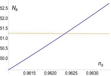
Figure 1: The solid (blue) curve represents the lhs of Eq. (3.4) while the dashed (orange) curve represents the slowly varying function of the rhs of the same equation. The intersection point gives us the value $n_{s}=0.96235$ for the scalar spectral index and, from the consistency relation for the Starobinsky model given by Eqs. (2.2), (4.2), (4.3), and (4.4), we obtain the other observables.

4 Observables and the number of $e$-folds

Using Eq. (2.8), which, when substituted in (2.9), relates $N_{k}$ to $n_{s}$, we can solve equation (3.4) directly for $n_{s}$ (see Fig. 1). This yields the following result

$$n_{s}=0.96235,$$ (4.1)

with the last digit rounded off. The consistency relations for the Starobinsky model [23] provide the following expressions for the tensor-to-scalar ratio $r$, the running of the spectral index $n_{sk}$, and the running of the tensor $n_{tk}$, in terms of $n_{s}$

$$r=\frac{4}{3}\left(2-2\sqrt{1+3\delta_{n_{s}}}+3\delta_{n_{s}}\right),$$ (4.2)

$$n_{sk}=\frac{1}{18}\left(4+9\delta_{n_{s}}-9\delta_{n_{s}}^{2}-\sqrt{1+3\delta_{n_{s}}}\left(4+3\delta_{n_{s}}\right)\right),$$ (4.3)

$$n_{tk}=\frac{1}{36}\left(8+3(4-3\delta_{n_{s}})\delta_{n_{s}}-8\sqrt{1+3\delta_{n_{s}}}\right),$$ (4.4)

where $\delta_{n_{s}}\equiv 1-n_{s}$, as before. Using these equations, we can compute the values for the other observables. We can also determine the number of $e$-folds of inflation, reheating and, from entropy conservation after reheating [24], the number of $e$-folds of radiation

$$N_{rd}\equiv\ln\left(\frac{a_{eq}}{a_{r}}\right)=\ln\left(\frac{a_{eq}T_{re}}{\left(\frac{43}{11g_{s,re}}\right)^{1/3}a_{0}T_{0}}\right),$$ (4.5)

where $a_{r}$ denotes the scale factor at the end of reheating or, equivalently, at the beginning of the radiation epoch and $a_{eq}$ is the scale factor at radiation-matter equality. Values of observables as well as number of $e$-folds are given in the Table 1.

Finally, we can use the expression

$$N_{keq}\equiv\ln\left(\frac{a_{eq}}{a_{k}}\right)=\ln\left(\frac{a_{e}}{a_{k}}\right)+\ln\left(\frac{a_{r}}{a_{e}}\right)+\ln\left(\frac{a_{eq}}{a_{r}}\right)=N_{k}+N_{re}+N_{rd},$$ (4.6)

as a consistency check. This equation can be written more concisely as $N_{keq}=\ln\left(\frac{a_{eq}H_{k}}{k_{p}}\right)=\ln\left(\frac{a_{eq}\pi\sqrt{A_{s}r}}{\sqrt{2}k_{p}}\right)$ [22]. We find that $N_{k}+N_{re}+N_{rd}\approx 113.182$, and the same value using the formula $N_{keq}=\ln\left(\frac{a_{eq}\pi\sqrt{A_{s}r}}{\sqrt{2}k_{p}}\right)$.

Parameter	Value	Parameter	Value
$k_{p}$	$0.05Mpc^{-1}$	$T_{re}$	$3.1\times 10^{9}\mathrm{GeV}$
$T_{0}$	$2.7255\,K$	$\phi_{e}$	$0.615M_{Pl}$
$A_{s}$	$2.1\times 10^{-9}$	$a_{eq}$	$2.9\times 10^{-4}$
Observable	Value	$e$-folds	Value
$n_{s}$	$0.96235$	$N_{k}$	$51.2$
$r$	$0.00403$	$N_{re}$	$18.0$
$n_{t}$	$-0.00050$	$N_{rd}$	43.9
$n_{sk}$	$-0.00072$	$N_{k}+N_{re}+N_{rd}$	113.2
$n_{tk}$	$-0.000019$	$N_{keq}$	$113.2$

Table 1: Above, we have listed the parameter values used in the calculations, while below, we present the values obtained for the observables and number of $e$-folds. Note that for $g_{re}\approx g_{s,re}$, Eq. (3.4) is practically independent of both $g_{re}$ and $g_{s,re}$. We solve Eq. (3.4) for the spectral index $n_{s}$, and by using the consistency relations given by (2.2), (4.2), (4.3), and (4.4), we obtain the other observables. The number of $e$-folds during inflation $N_{k}$, reheating $N_{re}$, and radiation $N_{rd}$ are calculated using the equations (2.9), (3.2), and (4.5), respectively. For an explanation about the presence of the term $N_{keq}$, see the last paragraph of Section 4. We observe that all the values obtained are within ranges calculated previously [23] and are in remarkable agreement with current measurements of the power spectrum of primordial curvature fluctuations and the present bounds on the spectrum of primordial gravitational waves.

5 Conclusions

Our approach allows us to find solutions for the cosmological observables, including the number of $e$-folds during inflation, reheating, and radiation, with minimal assumptions. By imposing the reheating conditions, we establish a connection between inflation and reheating and derive Eq. (3.4), which can be solved for the spectral index $n_{s}$. We utilize the consistency relations of the model to determine the values for the other observables. The number of $e$-folds during inflation $N_{k}$ and the number of $e$-folds during reheating $N_{re}$ are also determined by their respective formulas involving $n_{s}$, while the number of $e$-folds during radiation $N_{rd}$ is determined by the reheating temperature $T_{re}$. Our results demonstrate remarkable agreement between the Starobinsky model and current measurements of the power spectrum of primordial curvature fluctuations and the present bounds on the spectrum of primordial gravitational waves.

References

- [1] Alexei A. Starobinsky, A New Type of Isotropic Cosmological Models Without Singularity, Phys. Lett., B91:99–102, 1980.
- [2] Andrei D. Linde, The Inflationary Universe, Rept. Prog. Phys., 47:925–986, 1984.
- [3] David H. Lyth and Antonio Riotto, Particle physics models of inflation and the cosmological density perturbation, Phys. Rept., 314:1–146, 1999.
- [4] D. Baumann, Inflation, arXiv: 0907.5424 [hep-th].
- [5] Jerome Martin, The Theory of Inflation, In 200th Course of Enrico Fermi School of Physics: Gravitational Waves and Cosmology (GW-COSM) Varenna (Lake Como), Lecco, Italy, July 3-12, 2017, 2018.
- [6] B. A. Bassett, S. Tsujikawa and D. Wands, Inflation dynamics and reheating, Rev. Mod. Phys., 78, 537 (2006).
- [7] Rouzbeh Allahverdi, Robert Brandenberger, Francis-Yan Cyr-Racine, and Anupam Mazumdar, Reheating in Inflationary Cosmology: Theory and Applications, Ann. Rev. Nucl. Part. Sci., 60:27–51, 2010.
- [8] Mustafa A. Amin, Mark P. Hertzberg, David I. Kaiser, and Johanna Karouby, Nonperturbative Dynamics Of Reheating After Inflation: A Review, Int. J. Mod. Phys., D24:1530003, 2014.
- [9] Y. Akrami et al. [Planck Collaboration], Planck 2018 results. X. Constraints on inflation, Astron. Astrophys., 641(2020) A10.
- [10] P. A. R. Ade et al. [BICEP and Keck], Improved Constraints on Primordial Gravitational Waves using Planck, WMAP, and BICEP/Keck Observations through the 2018 Observing Season, Phys. Rev. Lett. 127, no.15, 151301 (2021).
- [11] M. Tristram, A. J. Banday, K. M. Górski, R. Keskitalo, C. R. Lawrence, K. J. Andersen, R. B. Barreiro, J. Borrill, L. P. L. Colombo and H. K. Eriksen, et al., Improved limits on the tensor-to-scalar ratio using BICEP and Planck data, Phys. Rev. D 105, no.8, 083524 (2022).
- [12] A. Vilenkin, Classical and Quantum Cosmology of the Starobinsky Inflationary Model, Phys. Rev. D 32, 2511 (1985).
- [13] T. Faulkner, M. Tegmark, E. F. Bunn and Y. Mao, Constraining f(R) Gravity as a Scalar Tensor Theory, Phys. Rev. D 76, 063505 (2007).
- [14] D.S. Gorbunov, and A.G. Panin, Scalaron the mighty: producing dark matter and baryon asymmetry at reheating, Phys. Lett. B 700,157, 2011.
- [15] Andrew R. Liddle, Paul Parsons, and John D. Barrow, Formalizing the slow roll approximation in inflation, Phys. Rev. D, 50: 7222–7232, 1994.
- [16] J. Ellis, M. A. G. Garcia, D. V. Nanopoulos and K. A. Olive, Calculations of Inflaton Decays and Reheating: with Applications to No-Scale Inflation Models, JCAP 07, 050 (2015).
- [17] Andrew R Liddle and Samuel M Leach, How long before the end of inflation were observable perturbations produced?, Phys. Rev., D68:103503, 2003.
- [18] Scott Dodelson, and Lam Hui, A Horizon ratio bound for inflationary fluctuations, Phys. Rev. Lett., 91, 131301, 2003.
- [19] Liang Dai, Marc Kamionkowski, and Junpu Wang, Reheating constraints to inflationary models, Phys. Rev. Lett., 113:041302, 2014.
- [20] Julian B. Munoz and Marc Kamionkowski, Equation of State Parameter for Reheating, Phys. Rev., D91(4):043521, 2015.
- [21] G. Germán, Constraining -attractor models from reheating, Int. J. Mod. Phys. D31 (10), 2250081, (2022).
- [22] G. Germán, Model independent results for the inflationary epoch and the breaking of the degeneracy of models of inflation, JCAP, 11(2020)006.
- [23] Marcos A. G. Garcia, G. Germán, Gonzalez Quaglia, R, A. M. Moran Colorado, Reheating constraints and consistency relations of the Starobinsky model and some of its generalizations, arXiv eprint, 2306.15831, astro-ph.CO.
- [24] G. Germán, Gonzalez Quaglia, R, Moran Colorado, A. M., Model independent bounds for the number of e-folds during the evolution of the universe, JCAP, 03(2023)004.