Mixed-state additivity properties of magic monotones based on quantum relative entropies for single-qubit states and beyond

Abstract

We prove that the stabilizer fidelity is multiplicative for the tensor product of an arbitrary number of single-qubit states. We also show that the relative entropy of magic becomes additive if all the single-qubit states but one belong to a symmetry axis of the stabilizer octahedron. We extend the latter results to include all the $\alpha$-$z$ Rényi relative entropy of magic. This allows us to identify a continuous set of magic monotones that are additive for single-qubit states. We also show that all the monotones mentioned above are additive for several standard two and three-qubit states subject to depolarizing noise. Finally, we obtain closed-form expressions for several states and tighter lower bounds for the overhead of probabilistic one-shot magic state distillation.

1 Introduction

The resource theory of magic provides a framework to quantify the advantage of quantum computation over classical computation [47]. In this setting, free resources lead to efficiently classically simulable computation, while resource states or ‘magic states’ unlock the quantum advantage over the classical counterpart allowing for universal quantum computation. The core idea is that by injecting magic states into the circuit, using only stabilizer operations, it is possible to implement non-stabilizer gates and achieve universal quantum computation. According to the Gottesman-Knill theorem [16], stabilizer operations can be efficiently classically simulated while the simulation runtime scales exponentially with the number of injected magic states into the circuit [1]. Magic monotones quantify the amount of magic resources contained in a quantum state. It turns out that the qudit magic theory for odd-dimensional Hilbert spaces is structurally simple [47, 18, 46, 28]. This is because the Wigner function is well-behaved. In this case, many monotones have been defined and multiplicativity is a common occurrence. Some prominent examples include the mana introduced in the seminal work [47] and the min and max-thauma introduced in [48]. However, despite many attempts, alternative ways of defining a well-behaved Wigner function for qubits suffer from drawbacks, and any attempt to define additive monotones for all qubit states proved to be highly challenging [40].

The relative entropy measure is often a common choice in resource theories since, once regularized, it provides upper bounds on asymptotic conversion rates between states in any convex resource theory [22]. In magic theory, the so-called relative entropy of magic was first introduced in [47]. However, although it was introduced almost a decade ago, its properties are known only for the few cases where it relates to other resource monotones [40, 42]. Another popular choice is the fidelity measure, which quantifies the resource of a state in terms of the infidelity from the set of free states. In the context of magic theory, it was introduced in [47] and it is known as stabilizer fidelity. Finally, we mention the generalized robustness of magic, which quantifies how much mixing with a state can take place before a magic state becomes a stabilizer state [26, 40]. The latter monotone benchmarks several proposed classical simulators (see [40] for more details). Moreover, for single-qubit states, the generalized robustness of magic is equal to the dyadic negativity and the mixed-state extent [40, Theorem 3]. The relative entropy of magic, the stabilizer fidelity, and the generalized robustness of magic are instances of magic monotones based on a quantum relative entropy and can be defined for any resource theory. A fundamental problem is whether the magic monotones based on a quantum relative entropy are additive under tensor products, and if not, under which conditions they become additive. However, very little is known about the additivity properties of these monotones. Besides its theoretical interest, the latter property is practically useful since it allows us to reduce the computation of the magic resource of the ‘whole’ to just the sum of one of the ‘parts’. The computation of these monotones becomes soon unfeasible for multi-qubit states as the number of qubits grows. This is because the number of pure stabilizer states scales super-exponentially with the number of qubits. For numerical experiments, we are limited to just five-qubit states [40, 24]. The additivity property allows us to overcome this problem for tensor products of low-dimensional multi-qubit states. In this case, the total magic resource just equals the sum of the one of each state, which is computable.

We now summarize the main results of this work.

• In Section 3, we prove that the stabilizer fidelity is multiplicative for tensor products of any number of single-qubit states. We then extend this result to include a continuous set of magic monotones, namely all the $\alpha$-$z$ Rényi relative entropies of magic in the range $|(1-\alpha)/z|=1$. In this way, we also independently recover the multiplicativity of the generalized robustness of magic for all single-qubit states established in [40].

• In Section 4, we prove that the relative entropy of magic is additive for single-qubit states if all of them but one commute with their optimizer, i.e. the closest stabilizer state. Moreover, in Section 8, we show that the latter class includes the $T$,$H$, and $F$ states subject to depolarizing noise. These are the states involved in the standard magic state distillation scenario where any initial state is first projected onto a symmetry axis of the octahedron by applying the stabilizer twirling, from which one aims to distill a better pure magic state [9, 10]. We extend this result to all the $\alpha$-$z$ Rényi relative entropies of magic. Finally, we also show that the relative entropy of magic is not additive for general two multi-qubit states by providing a counterexample.

• In Section 5, we prove that all the $\alpha$-$z$ Rényi relative entropies of magic are additive for two and three-qubit states that belong to a specific class. In Section 8, we show that the latter class includes the Toffoli, Hoggar, and $CS$ states subject to global depolarizing noise.

• In Section 6 we show that the $\alpha$-$z$ Rényi relative entropies of magic provide tighter probabilistic lower bounds near the deterministic region for the overhead of magic state distillation. The additivity results obtained in the previous sections extend these results to the case where multiple copies are involved in the process. Moreover, they extend these results to scenarios involving low dimensional catalysts that assist the transformation and could potentially provide a better overhead.

• In Section 7, we show that two additive quantities for single-qubit states, namely the generalized robustness and the stabilizer fidelity, have a closed for all single-qubit states. In Section 8 we give a closed-form for several two and three-qubit states belonging to the additivity classes for all the $\alpha$-$z$ Rényi relative entropies of magic. Explicitly, we consider $T,H,F$, Toffoli, Hoggar, and $CS$ magic states subject to global depolarizing noise.

• In Section 9, we show that for general odd-dimensional states, no monotone based on a quantum relative entropy is additive.

• Finally, in Section 10 we discuss a method that potentially could be useful to prove the additivity of the $\alpha$-$z$ Rényi relative entropies of magic in the range $|(1-\alpha)/z|=1$ for any number of any two and three-qubit states.

2 Magic states and magic monotones

We denote with $\mathcal{P}(A)$ the set of positive operators on a Hilbert space $A$. Moreover, we denote with $\mathcal{S}(A)$ the set of quantum states, i.e. the subset of $\mathcal{P}(A)$ with unit trace. A resource theory is defined by a set $\mathcal{F}$ of free states and a set $\mathcal{O}_{\mathcal{F}}$ of free operations with the property that map free states into free states [11, 5]. In the resource theory of magic, the free states are the set of stabilizer states $\mathcal{F}=\bar{S}$ [47]. The stabilizer states are defined as follows. The $n$-qubit Clifford group $\mathcal{C}_{n}$ is the group of $n$-qubit unitaries generated by the single-qubit gates H, S, and the CNOT two-qubit gate. Here, H is the Hadamed gate, S is the phase gate and CNOT is the controlled-not gate. The pure $n$-qubit stabilizer states are the ones generated by the Clifford group acting on $\ket{0^{n}}$, i.e. all the states $S_{n}=\{U\ket{0^{n}}:U\in\mathcal{C}_{n}\}$. The set of all (mixed) stabilizer states is formed by all convex combinations (convex hull) of pure stabilizer states, $\bar{S}_{n}:=\text{conv}\{\outerproduct{\psi}{\psi}:\ket{\psi}\in S_{n}\}$. We omit the subscript $n$ if the geometry is clear from the context. We say that a state $\rho$ is magic if it is not a stabilizer state.

In this work, we mainly focus on single-qubit states. We say that a pure state $\ket{\psi}$ is stabilized by an operator $P$ if $P\ket{\psi}=\ket{\psi}$. The single-qubit pure stabilizer states are the states that are stabilized by the Pauli operators as well as their products with $\pm\mathds{1}$. These are the states $\ket{0}$, $\ket{1}$, $\ket{+}:=(\ket{0}+\ket{1})/\sqrt{2}$, $\ket{-}:=(\ket{0}-\ket{1})/\sqrt{2}$, $\ket{+i}:=(\ket{0}+i\ket{1})/\sqrt{2}$, $\ket{-i}:=(\ket{0}-i\ket{1})/\sqrt{2}$. The set of all the stabilizer states in the Bloch sphere forms an octahedron whose vertexes are the pure stabilizer states. In this work, we mainly focus on multi-qubit systems. The resource theory of magic can also be formulated for higher-dimensional qudit systems. We refer to [47, 9] for a formal definition. In the following, we sometimes consider some standard magic states subject to depolarizing noise. The depolarizing channel is defined by the map

$$\Delta_{p}:\rho\rightarrow p\rho+(1-p)\frac{\mathds{1}}{d},$$ (1)

where $p\in[0,1]$.

Resource monotones quantify the resource of a quantum state. We call a function $\mathfrak{R}:\mathcal{S}(A)\rightarrow[0,+\infty]$ a resource monotone if it does not increase under free operations, i.e., if $\mathfrak{R}(\rho)\geq\mathfrak{R}(\mathcal{E}(\rho))$ for any state $\rho$ and any free operation $\mathcal{E}\in\mathcal{O}_{\mathcal{F}}$. In the resource theory of magic, resource monotones are called magic monotones. In this work, we will mainly be concerned with the magic monotones based on the $\alpha$-$z$ Rényi relative entropies. This allows us to address in a compact way several magic monotones already introduced in the literature. Although there are several ways to define free operations in the resource theory of magic [47, 39, 40], in this work we do not specify any set of free operations since the $\alpha$-$z$ Rényi relative entropies of magic are monotone for any choice of free operations. We say that $\mathfrak{R}$ is tensor sub-additive (or just sub-additive) for the states $\rho_{1}$ and $\rho_{2}$ if $\mathfrak{R}(\rho_{1}\otimes\rho_{2})\leq\mathfrak{R}(\rho_{1})+\mathfrak{R}(\rho_{2})$. Moreover, we say that $\mathfrak{R}$ is tensor additive (or just additive) for the states $\rho_{1}$ and $\rho_{2}$ if $\mathfrak{R}(\rho_{1}\otimes\rho_{2})=\mathfrak{R}(\rho_{1})+\mathfrak{R}(\rho_{2})$.

We now introduce the $\alpha$-$z$ Rényi relative entropies. Let $\alpha\in(0,1)\cup(1,\infty),\;z>0$, $\rho\in\mathcal{S}(A)$ and $\sigma\in\mathcal{P}(A)$. Then the $\alpha$-$z$ Rényi relative entropy of $\sigma$ with $\rho$ is defined as [2, 50]

$$D_{\alpha,z}(\rho\|\sigma):=\begin{cases}\frac{1}{\alpha-1}\log{\text{Tr}\left(\rho^{\frac{\alpha}{2z}}\sigma^{\frac{1-\alpha}{z}}\rho^{\frac{\alpha}{2z}}\right)^{z}}&\text{if}\;(\alpha<1\wedge\rho\not\perp\sigma)\vee\rho\ll\sigma\\ +\infty&\text{else}\end{cases}\,.$$ (2)

In the following, we denote

$$Q_{\alpha,z}(\rho\|\sigma):=\exp\big((\alpha-1)D_{\alpha,z}(\rho\|\sigma)\big{missing})\,.$$ (3)

In the limit points of the ranges of the parameters, we define the $\alpha$-$z$ Rényi relative entropy by taking the corresponding pointwise limits. In particular, throughout the text, we will often be concerned with the pointwise limits

$$D_{\min}(\rho\|\sigma)=\lim\limits_{\alpha\rightarrow 0}D_{\alpha,1-\alpha}(\rho\|\sigma)\;,\;D(\rho\|\sigma)=\lim\limits_{\alpha\rightarrow 1}D_{\alpha,\alpha}(\rho\|\sigma)\;,D_{\max}(\rho\|\sigma)=\lim\limits_{\alpha\rightarrow\infty}D_{\alpha,\alpha-1}(\rho\|\sigma)\,,$$ (4)

where

$$D_{\min}(\rho\|\sigma):=-\log{\Tr(\Pi(\rho)\sigma)}\,,$$ (5)

$$D(\rho\|\sigma):=\Tr(\rho(\log{\rho}-\log{\sigma}))\,,\,\text{and}$$ (6)

$$D_{\max}(\rho\|\sigma):=\inf\{\lambda\in\mathbb{R}:\rho\leq 2^{\lambda}\sigma\}\,,$$ (7)

are the min-relative entropy [36, 12], the Umegaki relative entropy, and the max-relative entropy [43, 12, 36], respectively. In Appendix D, we prove the first and the third limit of (4). Note that the second limit in (4) for the Umegaki relative entropy holds for any $z>0$ [25]. Here, we denoted with $\Pi(\rho)$ the projector onto the support of $\rho$.

In [50, Theorem 1.2], the author proved that the $\alpha$-$z$ Rényi relative entropy satisfies the data-processing inequality (DPI) for the following range of parameters

1. $\quad 0<\alpha<1\;\;and\;\;z\geq\max\{\alpha,1-\alpha\},$

2. $\quad 1<\alpha\leq 2\;\;and\;\;\frac{\alpha}{2}\leq z\leq\alpha,\;and$

3. $\quad 2\leq\alpha<\infty\;\;and\;\;\alpha-1\leq z\leq\alpha\,.$

We denote with $\mathcal{D}$ the set of above values of the parameters $(\alpha,z)$ for which the $D_{\alpha,z}$ satisfies the DPI. Because of the limits in (4), the $\alpha$-$z$ Rényi relative entropy also satisfies the DPI on the line $\alpha=1$. We include this line in the region $\mathcal{D}$. In Fig. 1, we represent in blue the region for which the $\alpha$-$z$ Rényi relative entropies satisfy the DPI.

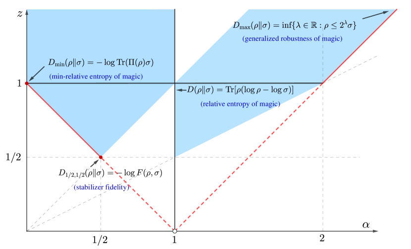
Figure 1: $\alpha$-$z$ plane for the $\alpha$-$z$ Rényi relative entropies. The vertical line $\alpha=1$ for $z>0$ corresponds to the Umegaki relative entropy. The blue region (together with the Umegaki relative entropy line) is where the data-processing inequality holds. We show in red the special line $|(1-\alpha)/z|=1$ located at the boundary of the DPI region. We write in blue the related magic monotones associated with the respective points. In Section 6 we use the additivity of the monotones in a neighborhood of $\alpha=0,z=1$ (circled in red) to obtain tighter one-shot bounds for magic state distillation.

We define magic monotones for $(\alpha,z)\in\mathcal{D}$ as

$$\mathfrak{D}_{\alpha,z}(\rho):=\inf_{\sigma\in\bar{S}}D_{\alpha,z}(\rho\|\sigma)\,.$$ (8)

Analogously, we denote

$$\mathcal{Q}_{\alpha,z}(\rho):=\exp\big((\alpha-1)\mathfrak{D}_{\alpha,z}(\rho)\big{missing})\,.$$ (9)

In the following, we call these monotones Rényi relative entropies of magic. In particular, we have

$$\mathfrak{D}_{\min}(\rho):=\inf_{\sigma\in\bar{S}}D_{\min}(\rho\|\sigma),\quad\mathfrak{D}(\rho):=\inf_{\sigma\in\bar{S}}D(\rho\|\sigma),\quad\mathfrak{D}_{\max}(\rho):=\inf_{\sigma\in\bar{S}}D_{\max}(\rho\|\sigma)\,.$$ (10)

Note that since the $\alpha$-$z$ Rényi relative entropies are lower semicontinuous, we can replace the above infimum with a minimum [37]. In Appendix D we prove that we can recover the latter monotones as pointwise limits of the monotone (8). Namely, we have

$$\mathfrak{D}_{\min}(\rho)=\lim\limits_{\alpha\rightarrow 0}\mathfrak{D}_{\alpha,1-\alpha}(\rho),\quad\mathfrak{D}(\rho)=\lim\limits_{\alpha\rightarrow 1}\mathfrak{D}_{\alpha,\alpha}(\rho),\quad\mathfrak{D}_{\max}(\rho)=\lim\limits_{\alpha\rightarrow\infty}\mathfrak{D}_{\alpha,\alpha-1}(\rho)\,.$$ (11)

The $\mathfrak{D}_{\alpha,z}$ do not increase under any set of free operations that map stabilizer states into stabilizer states, i.e. they are indeed magic monotones. The latter property is a straightforward consequence of the fact that the underlying $D_{\alpha,z}$ satisfies the data-processing inequality. Moreover, it is easy to prove that the $\mathfrak{D}_{\alpha,z}$ are sub-additive for general states.

The $\alpha$-$z$ Rényi relative entropies encompass many well-known quantities. The relative entropy of magic was first introduced in the seminal work [47] and was the first monotone based on a quantum relative entropy to be proposed. The relative entropy of magic is equal to $\mathfrak{D}$ defined in (10). The stabilizer fidelity was first introduced in [6] and is defined as

$$\mathfrak{F}(\rho)=\sup\limits_{\sigma\in\bar{S}}F(\rho,\sigma)\,,$$ (12)

where $F(\rho,\sigma):=(\text{Tr}|\sqrt{\rho}\sqrt{\sigma}|)^{2}$ is the Uhlmann’s fidelity. We have the relationship $\mathfrak{D}_{1/2,1/2}(\rho)=-\log{\mathfrak{F}(\rho)}$. The generalized robustness of magic was later introduced in [26, 40] and it is defined as

$$\Lambda^{+}(\rho):=\inf\left\{s\geq 1:\exists\omega\in\mathcal{S}(A)\,\,\text{s.t}\,\,\frac{1}{s}\left(\rho+(s-1)\omega\right)\in\bar{S}\right\}\,.$$ (13)

The generalized robustness of magic is connected to the monotone based on the max-relative entropy through the relation $\mathfrak{D}_{\max}(\rho)=\log{(\Lambda^{+}(\rho))}$. In Fig. 1 we show where the latter monotones are located in the $\alpha$-$z$ plane. We show in red the boundary of the DPI region $|(1-\alpha)/z|=1$. Notably, the latter line contains the stabilizer fidelity, the min, and the max-relative entropy of magic. As we discuss below, these monotones on the boundary satisfy stronger additivity properties than the one located at the interior of the DPI region.

For a monotone to be called an entanglement measure, further properties such as faithfulness, convexity, or strong monotonicity are usually required [23, 44, 45]. As we discuss in Appendix B, the relative entropy of magic, the stabilizer fidelity, and the generalized robustness of magic satisfy these properties. Moreover, for any $(\alpha,z)\in\mathcal{D}$ it is possible to construct quantities with these desired properties. This fact is very general and holds for a wide class of resource theories. In particular, in Section 6 we will use the monotonicity under probabilistic distillation protocols to find lower bounds for probabilistic magic state distillation.

In the next sections, we focus on the additivity properties of the magic monotones based on the $\alpha$-$z$ Rényi relative entropies. Note that we can restrict our attention only to magic states. Indeed, for free states, additivity readily follows from data processing under partial trace and sub-additivity of the monotones as noted in [47, Theorem 7].

3 Additivity of the $\alpha$-$z$ Rényi relative entropies of magic in the range $|(1-\alpha)/z|=1$ for all single-qubit states

In this section, we prove that the stabilizer fidelity is multiplicative for an arbitrary number of tensor products of single-qubit states. Previously, it was known only for pure states [6]. We generalize the result for all the $\alpha$-$z$ Rényi relative entropies of magic in the region $|(1-\alpha)/z|=1$. In this way, by taking the limit $\alpha\rightarrow\infty$ and $\alpha\rightarrow 0$, we independently recover the multiplicativity of the generalized robustness of magic and the additivity of the $\mathfrak{D}_{\min}$ established in [40] and [38], respectively.

The key ingredient for the proof of the stabilizer fidelity is the multiplicativity for all single-qubit states of the linear functional

$$\mathfrak{F}_{0}(\rho):=\max\limits_{\sigma\in\bar{S}}\text{Tr}(\rho\sigma)\,.$$ (14)

Note that the above function is simpler than the fidelity due to its linearity. As we show later, the multiplicativity of the above quantity is tightly connected to the one of the stabilizer fidelity.

We now show that $\mathfrak{F}_{0}$ is multiplicative for an arbitrary number of single-qubit states.

Proposition 1.

Let $\{\rho_{i}\}_{i=1}^{L}$ be a set of single-qubit states. Then, we have

$$\mathfrak{F}_{0}\left(\bigotimes_{i=1}^{L}\rho_{i}\right)=\prod_{i=1}^{L}\mathfrak{F}_{0}(\rho_{i})\,.$$ (15)

Proof.

Let $r_{i}=(x_{i},y_{i},z_{i})$ be the Bloch vectors of $\rho_{i}$ for $i=1,2$. Without loss of generality, since $\mathfrak{F}_{0}$ is invariant under Clifford unitaries, let us assume that $z_{i}\geq y_{i}\geq x_{i}\geq 0$. Using the spectral decomposition, we can decompose any qubit state as a convex combination between a pure state and the identity. Indeed, we have

$$\rho=p\psi_{r}+(1-p)\psi_{-r}=(2p-1)\psi_{r}+(1-p)\mathds{1}\,,$$ (16)

where we denoted with $\psi_{r}$ and $\psi_{-r}$ the eigenvectors of $\rho$. Note that, by assumption, $p\geq 1/2$. We, therefore, obtain that

$$\mathfrak{F}_{0}(\rho) =\max\limits_{\sigma\in\bar{S}}\text{Tr}(\rho\sigma)$$ (17)

$$=(2p-1)\max\limits_{\sigma\in\bar{S}}\text{Tr}(\psi_{r}\sigma)+(1-p)$$ (18)

$$=a\mathfrak{F}_{0}(\psi_{r})+b\,,$$ (19)

where we defined the positive constant $a:=(2p-1)$ and $b:=(1-p)$. Hence, the optimum is achieved by the state that maximizes the overlap with the pure state in the decomposition with the highest weight. We now consider the tensor product of two states. Using the above decomposition for both states, we obtain

$$\mathfrak{F}_{0}(\rho_{1}\otimes\rho_{2})= a_{1}a_{2}\text{Tr}(\tau\psi_{r_{1}}\otimes\psi_{r_{2}})+a_{1}b_{2}\text{Tr}(\text{Tr}_{2}(\tau)\psi_{r_{1}})+b_{1}a_{2}\text{Tr}(\text{Tr}_{1}(\tau)\psi_{r_{2}})+b_{1}b_{2}$$ (20)

$$\leq a_{1}a_{2}\mathfrak{F}_{0}(\psi_{r_{1}})\mathfrak{F}_{0}(\psi_{r_{2}})+a_{1}b_{2}\mathfrak{F}_{0}(\psi_{r_{1}})+b_{1}a_{2}\mathfrak{F}_{0}(\psi_{r_{2}})+b_{1}b_{2}$$ (21)

$$= (a_{1}\mathfrak{F}_{0}(\psi_{r_{1}})+b_{1})(a_{2}\mathfrak{F}_{0}(\psi_{r_{2}})+b_{2})$$ (22)

$$= \mathfrak{F}_{0}(\rho_{1})\mathfrak{F}_{0}(\rho_{2})\,,$$ (23)

where we used $\rho_{1,2}=a_{1,2}\psi_{r_{1,2}}+b_{1,2}\mathds{1}$. Here, we denoted with $\tau$ the optimizer of $\rho_{1}\otimes\rho_{2}$. Moreover, we used that, for pure states, $\mathfrak{F}_{0}$ is equal to the stabilizer fidelity and the latter is multiplicative for an arbitrary number of pure states [6]. We also used that the partial trace of a free state is a free state since the partial trace is a free operation. In the last equality, we used equation (19). Note that we always have $\mathfrak{F}_{0}(\rho_{1}\otimes\rho_{2})\geq\mathfrak{F}_{0}(\rho_{1})\mathfrak{F}_{0}(\rho_{2})$ since $\mathfrak{F}_{0}$ is super-multiplicative. Hence, we have that $\mathfrak{F}_{0}(\rho_{1}\otimes\rho_{2})=\mathfrak{F}_{0}(\rho_{1})\mathfrak{F}_{0}(\rho_{2})$. The proof for the tensor product of more than two qubits follows similarly. ∎

We now show that all the $\alpha$-$z$ Rényi relative entropies of magic are additive for single-qubit states in the range $|(1-\alpha)/z|=1$. The result for $\alpha=z=1/2$ implies that the stabilizer fidelity is multiplicative for tensor products of any single-qubit states.

Theorem 2.

Let $(\alpha,z)\in\mathcal{D}$ such that $|(1-\alpha)|/z=1$. Moreover, let $\{\rho_{i}\}_{i=1}^{L}$ be a set of single-qubit states. Then, we have

$$\mathfrak{D}_{\alpha,z}\left(\bigotimes_{i=1}^{L}\rho_{i}\right)=\sum_{i=1}^{L}\mathfrak{D}_{\alpha,z}(\rho_{i})\,.$$ (24)

Proof.

We first start by considering the tensor product of two-qubit states $\rho_{1}$ and $\rho_{2}$. To prove multiplicativity, we show that $\tau_{1}\otimes\tau_{2}\in\operatorname*{arg\,min}_{\sigma\in\bar{S}}D_{\alpha,z}(\rho_{1}\otimes\rho_{2}\|\sigma)$ if $\tau_{1}$ and $\tau_{2}$ are some optimizers of the marginal problems, i.e. $\tau_{1}\in\operatorname*{arg\,min}_{\sigma\in\bar{S}}D_{\alpha,z}(\rho_{1}\|\sigma)$ and $\tau_{2}\in\operatorname*{arg\,min}_{\sigma\in\bar{S}}D_{\alpha,z}(\rho_{2}\|\sigma)$. Since the $D_{\alpha,z}$ are additive, the latter condition implies the additivity of the related monotones. Indeed, we have $\mathfrak{D}_{\alpha,z}(\rho_{1}\otimes\rho_{2})=D_{\alpha,z}(\rho_{1}\otimes\rho_{2}\|\tau_{1}\otimes\tau_{2})=D_{\alpha,z}(\rho_{1}\|\tau_{1})+D_{\alpha,z}(\rho_{2}\|\tau_{2})=\mathfrak{D}_{\alpha,z}(\rho_{1})+\mathfrak{D}_{\alpha,z}(\rho_{2})$. Therefore, to prove additivity, according to Theorem 17 in Appendix A, we need to show that

$$\text{Tr}(\sigma\Xi_{\alpha,z}(\rho_{1}\otimes\rho_{2},\tau_{1}\otimes\tau_{2}))\leq Q_{\alpha,z}(\rho_{1}\otimes\rho_{2}\|\tau_{1}\otimes\tau_{2})=Q_{\alpha,z}(\rho_{1}\|\tau_{1})Q_{\alpha,z}(\rho_{2}\|\tau_{2}),\quad\forall\sigma\in\bar{S}\,.$$ (25)

We define the positive operator $\Xi_{\alpha,z}(\rho,\tau)$ in Appendix A. In the last equality, we used that the $Q_{\alpha,z}$ are multiplicative. Note that we always have that $\tau_{1}\otimes\tau_{2}$ satisfies the support conditions since, by assumption, the states $\tau_{1}$ and $\tau_{2}$ are optimizers of the marginal problems and hence satisfy them.

We then have, for any $\sigma\in\bar{S}$,

$$\text{Tr}(\sigma\Xi_{\alpha,z}(\rho_{1}\otimes\rho_{2},\tau_{1}\otimes\tau_{2})) \leq\max\limits_{\sigma\in\bar{S}}\text{Tr}(\sigma\Xi_{\alpha,z}(\rho_{1}\otimes\rho_{2},\tau_{1}\otimes\tau_{2}))$$ (26)

$$=\max\limits_{\sigma\in\bar{S}}\text{Tr}(\sigma\Xi_{\alpha,z}(\rho_{1},\tau_{1})\otimes\Xi_{\alpha,z}(\rho_{2},\tau_{2}))$$ (27)

$$=C_{1,\alpha,z}C_{2,\alpha,z}\max\limits_{\sigma\in\bar{S}}\text{Tr}(\sigma\widehat{\Xi}_{\alpha,z}(\rho_{1},\tau_{1})\otimes\widehat{\Xi}_{\alpha,z}(\rho_{2},\tau_{2}))$$ (28)

$$=C_{1,\alpha,z}C_{2,\alpha,z}\max\limits_{\sigma\in\bar{S}}\text{Tr}(\sigma\widehat{\Xi}_{\alpha,z}(\rho_{1},\tau_{1}))\max\limits_{\sigma\in\bar{S}}\text{Tr}(\sigma\widehat{\Xi}_{\alpha,z}(\rho_{2},\tau_{2}))$$ (29)

$$=\max\limits_{\sigma\in\bar{S}}\text{Tr}(\sigma\Xi_{\alpha,z}(\rho_{1},\tau_{1}))\max\limits_{\sigma\in\bar{S}}\text{Tr}(\sigma\Xi_{\alpha,z}(\rho_{2},\tau_{2}))$$ (30)

$$=\;Q_{\alpha,z}(\rho_{1}\|\tau_{1})Q_{\alpha,z}(\rho_{2}\|\tau_{2})\,,$$ (31)

where we defined the positive constants $C_{i,\alpha,z}:=\text{Tr}(\Xi_{\alpha,z}(\rho_{i},\tau_{i}))$ for $i=1,2$, and for a positive semidefinite operator $A$ we defined the quantum state $\widehat{A}:=A/\text{Tr}(A)$. In (27) we used that for $|(1-\alpha)/z|=1$, it holds $\Xi_{\alpha,z}(\rho_{1}\otimes\rho_{2},\tau_{1}\otimes\tau_{2})=\Xi_{\alpha,z}(\rho_{1},\tau_{1})\otimes\Xi_{\alpha,z}(\rho_{2},\tau_{2})$ (see Appendix A). In (29) we used the multiplicativity result in Proposition 1. The last equality follows from the fact that $\tau_{1}$ and $\tau_{2}$ are, by assumptions, optimizers of the marginal problems. Indeed, from Theorem 17, if $\tau\in\operatorname*{arg\,min}_{\sigma\in\bar{S}}Q_{\alpha,z}(\rho\|\sigma)$, we have that $\text{Tr}(\sigma\Xi_{\alpha,z}(\rho,\tau))\leq Q_{\alpha,z}(\rho\|\tau)$ for any $\sigma\in\bar{S}$. It is easy to see that the latter inequality is saturated for $\sigma=\tau$. The latter chain of inequalities proves the inequality (25). The proof for more than two qubits follows similarly. ∎

In the next section, we prove that for states that commute with their optimizer, we can prove additivity for all the range $(\alpha,z)\in\mathcal{D}$. In particular, the latter range contains the relative entropy of magic. We show in the Appendix that the single-qubit states that commute with its optimizer are the noisy (depolarized) $T$,$H$, and $F$ states.

4 Additivity of all the $\alpha$-$z$ Rényi relative entropies of magic for a specific class of single-qubit states

In this section, we show that the relative entropy of magic is additive for single-qubit states when all of them commute with their optimizer. Note that we actually show something slightly stronger. Indeed, we do not require one of the states to commute with its optimizer. In Section 8.1, we show that the single-qubit states that commute with its optimizer are the $T,H$, or $F$ states subject to depolarizing noise. Previously, additivity was known only for pure $H,T$, and $F$ states. Indeed, in this case, the relative entropy of magic equals both the stabilizer fidelity and the generalized robustness of magic, which are both additive for single-qubit pure states [6, 40].

We extend this result to include all the $\alpha$-$z$ Rényi relative entropy of magic for all $(\alpha,z)\in\mathcal{D}$. At the end of the section, we show that there exist two single-qubit states for which the relative entropy of magic is not additive. This shows that, unlike the fidelity or the robustness measure, the relative entropy one is not additive for tensor products of any single-qubit states.

Theorem 3.

Let $(\alpha,z)\in\mathcal{D}$ and let $\{\rho_{i}\}_{i=L}^{L}$ be a set of single-qubit states. Moreover, let $\tau_{i}\in\operatorname*{arg\,min}_{\sigma\in\bar{S}}D_{\alpha,z}(\rho_{i}\|\sigma)$. If $[\rho_{i},\tau_{i}]=0$ for any $i\in\{1,...,L-1\}$, then we have that

$$\mathfrak{D}_{\alpha,z}\left(\bigotimes_{i=1}^{L}\rho_{i}\right)=\sum_{i=1}^{L}\mathfrak{D}_{\alpha,z}(\rho_{i})\,.$$ (32)

Proof.

The proof is similar to the one of Theorem 2. We first start by considering the tensor product of two single-qubit states $\rho_{1}$ and $\rho_{2}$. In particular, we show that if $\tau_{1}$ is an optimizer of $\rho_{1}$ such that $[\rho_{1},\tau_{1}]=0$, then an optimizer of $\rho_{1}\otimes\rho_{2}$ is $\tau_{1}\otimes\tau_{2}$ where $\tau_{2}$ is any optimizer of $\rho_{2}$. According to Theorem 17, we want to show that

$$\text{Tr}(\sigma\Xi_{\alpha,z}(\rho_{1}\otimes\rho_{2},\tau_{1}\otimes\tau_{2}))\leq Q_{\alpha}(\rho_{1}\|\tau_{1})Q_{\alpha,z}(\rho_{2}\|\tau_{2})\,,\quad\forall\sigma\in\bar{S}\,,$$ (33)

where we denoted with $\tau_{1}$ and $\tau_{2}$ some optimizers of $\rho_{1}$ and $\rho_{2}$, respectively.

We now show that if $[\rho_{1},\tau_{1}]=0$, then we have $\Xi_{\alpha,z}(\rho_{1}\otimes\rho_{2},\tau_{1}\otimes\tau_{2})=\Xi_{\alpha,z}(\rho_{1},\tau_{1})\otimes\Xi_{\alpha,z}(\rho_{2},\tau_{2})$. This fact has been pointed out in the proof of Theorem 7 in [37]. We reprove it here for completeness. We use the spectral decomposition $\tau_{1}=\sum_{l}t_{1,l}|\psi_{l}\rangle\!\langle\psi_{l}|$ and $\tau_{2}=\sum_{r}t_{2,r}|\xi_{r}\rangle\!\langle\xi_{r}|$. Here, $|\psi_{l}\rangle$ is the common eigenbasis of $\rho_{1}$ and $\tau_{1}$. We have

$$\Xi_{\alpha,z}(\rho_{1}\otimes\rho_{2},\tau_{1}\otimes\tau_{2})$$ (34)

$$\qquad=\,K_{\alpha,z}\sum\limits_{l,r_{1},r_{2}}\int_{0}^{\infty}\left(t_{1,l}t_{2,r_{1}}+k\right)^{-1}\left(t_{1,l}t_{2,r_{2}}+k\right)^{-1}k^{\frac{1-\alpha}{z}}\mathrm{d}k\;\;|\psi_{l}\rangle\!\langle\psi_{l}|\chi_{\alpha,z}(\rho_{1},\tau_{1})|\psi_{l}\rangle\!\langle\psi_{l}|\;$$

$$\qquad\quad\otimes|\xi_{r_{1}}\rangle\!\langle\xi_{r_{1}}|\chi_{\alpha,z}(\rho_{2},\tau_{2})|\xi_{r_{2}}\rangle\!\langle\xi_{r_{2}}|$$ (35)

$$\qquad=\,K_{\alpha,z}\sum\limits_{l}t_{1,l}^{\frac{1-\alpha}{z}-1}|\psi_{l}\rangle\!\langle\psi_{l}|\chi_{\alpha,z}(\rho_{1},\tau_{1})|\psi_{l}\rangle\!\langle\psi_{l}|\;$$

$$\qquad\quad\otimes\sum_{r_{1},r_{2}}\int_{0}^{\infty}\left(t_{2,r_{1}}+k\right)^{-1}\left(t_{2,r_{2}}+k\right)^{-1}k^{\frac{1-\alpha}{z}}\mathrm{d}k|\xi_{r_{1}}\rangle\!\langle\xi_{r_{1}}|\chi_{\alpha,z}(\rho_{2},\tau_{2})|\xi_{r_{2}}\rangle\!\langle\xi_{r_{2}}|$$ (36)

$$\qquad=\;\rho_{1}^{\alpha}\tau_{1}^{-\alpha}\otimes\Xi_{\alpha,z}(\rho_{2},\tau_{2})$$ (37)

$$\qquad=\;\Xi_{\alpha,z}(\rho_{1},\tau_{1})\otimes\Xi_{\alpha,z}(\rho_{2},\tau_{2})\,,$$ (38)

where in the second equality we changed the measure $k\rightarrow t_{1,l}k$. Moreover, in (37) we used that $\sum_{k}t_{1,l}^{\frac{1-\alpha}{z}-1}|\psi_{l}\rangle\!\langle\psi_{l}|\chi_{\alpha,z}(\rho_{1},\tau_{1})|\psi_{l}\rangle\!\langle\psi_{l}|=\rho_{1}^{\alpha}\tau_{1}^{-\alpha}$. In the last equality, we used that if $[\rho_{1},\tau_{1}]=0$ then $\Xi_{\alpha,z}(\rho_{1},\tau_{1})=\rho^{\alpha}_{1}\tau_{1}^{-\alpha}$.

Following the same arguments to the proof of Theorem 2, the above result implies that for any $\sigma\in\bar{S}$ we have $\Tr(\sigma\Xi_{\alpha,z}(\rho_{1}\otimes\rho_{2},\tau_{1}\otimes\tau_{2}))\leq Q_{\alpha}(\rho_{1}\|\tau_{1})Q_{\alpha,z}(\rho_{2}\|\tau_{2})$. The latter inequality proves the inequality (33). The proof for more than two qubits follows similarly by noting that $\Xi_{\alpha,z}(\bigotimes_{i=1}^{L}\rho_{i},\bigotimes_{i=1}^{L}\tau_{i})=\bigotimes_{i=1}^{L}\Xi_{\alpha,z}(\rho_{i},\tau_{i})$ if $[\rho_{i},\tau_{i}]=0$ for any $i\in\{1,\ldots,L-1\}$ . ∎

4.1 Counterexample to the additivity of the relative entropy of magic for two multi-qubit states

We give new examples of the non-additivity of the relative entropy of magic for single-qubit states. Let us consider the pure state $\rho$ with Bloch vector $\vec{r}=((6+2\sqrt{3})^{-\frac{1}{2}},(6+2\sqrt{3})^{-\frac{1}{2}},(3-\sqrt{3})^{-\frac{1}{2}})$. We obtain numerically $\mathfrak{D}(\rho\otimes\rho)-2\mathfrak{D}(\rho)\approx-0.002121$. This shows that the relative entropy of magic is not additive for general two single-qubit states. However, we proved in Theorem 3 that additivity holds if at least one of the two states belongs to a symmetry axis of the stabilizer octahedron. We also note that at most one of the states can be of general form. Indeed, we numerically find $\mathfrak{D}(\outerproduct{F}{F}\otimes\rho\otimes\rho)-(\mathfrak{D}(\outerproduct{F}{F})+2\mathfrak{D}(\rho))\approx-0.002121$. Here, we denoted with $\outerproduct{F}{F}$ the pure state defined in equation (8.1) and we take $\rho$ as above. Further examples that violate the additivity property could be easily found also for multi-qubit states.

5 Additivity of all the $\alpha$-$z$ Rényi relative entropies of magic for a specific class of two and three-qubit states

In this section, we prove that for a specific class of mixed two and three-qubit states, all the $\alpha$-$z$ Rényi relative entropies of magic are additive. Previously, it was known that all the monotones in the line $|(1-\alpha)/z|=1$ are additive for pure states that describe a system of at most three qubits. Indeed, in the case of pure states, for $z=1-\alpha$ and $z=\alpha-1$, the $\alpha$-$z$ Rényi relative entropies of magic equal the log-stabilizer fidelity and the generalized log-robustness of magic, respectively. Then additivity is a consequence of multiplicativity of the stabilizer fidelity [6, Theorem 5] and the one of the stabilizer extent [6, Proposition 1] which for pure states equals the generalized robustness [32]. Since any monotone based on a quantum relative entropy is contained between $\mathfrak{D}_{\min}$ and $\mathfrak{D}_{\max}$ [17], for pure states $\rho$ such that $\mathfrak{D}_{\min}(\rho)=\mathfrak{D}_{\max}(\rho)$, the latter result can be extended to any monotone based on a quantum relative entropy. In the following, we address a specific class of mixed two and three-qubit states. In Section 8, we show that the latter class includes the Toffoli, Hoggar, and $CS$ states subject to global depolarizing noise.

Theorem 4.

Let $(\alpha,z)\in\mathcal{D}$ and $\{\rho_{i}\}_{i=L}^{L}$ be a set of states that describe a system of at most three qubits such that $\rho_{i}=\Delta_{p_{i}}(\outerproduct{\psi_{i}}{\psi_{i}})$ for some $p_{i}\geq 0$ and a pure state $\outerproduct{\psi_{i}}{\psi_{i}}$ for all $i=1,..,L$. Moreover, let $\tau_{i}\in\operatorname*{arg\,min}_{\sigma\in\bar{S}}D_{\alpha,z}(\rho_{i}\|\sigma)$. If $\tau_{i}=\Delta_{t_{i}}(\rho_{i})$ for some $t_{i}\geq 0$ for all $i=1,..,L$, then we have that

$$\mathfrak{D}_{\alpha,z}\left(\bigotimes_{i=1}^{L}\rho_{i}\right)=\sum_{i=1}^{L}\mathfrak{D}_{\alpha,z}(\rho_{i})\,.$$ (39)

Proof.

By assumption, we have $\rho_{i}=\Delta_{p_{i}}(\outerproduct{\psi_{i}}{\psi_{i}})$ and $\tau_{i}=\Delta_{t_{i}}(\outerproduct{\psi_{i}}{\psi_{i}})$ for some state $\outerproduct{\psi_{i}}{\psi_{i}}$ and parameters $p_{i}$ and $t_{i}$. Since $[\rho_{i},\tau_{i}]=0$, we check the conditions of Corollary 18. We have

$$\Xi_{\alpha}(\rho_{i},\tau_{i})=(a_{i}-b_{i})\outerproduct{\psi_{i}}{\psi_{i}}+b_{i}\mathds{1}\,,$$ (40)

where

$$a_{i}=\left(\frac{1+(d-1)p_{i}}{1+(d-1)t_{i}}\right)^{\alpha},\quad b_{i}=\left(\frac{1-p_{i}}{1-t_{i}}\right)^{\alpha}\,.$$ (41)

Note that, as discussed at the end of Section 2 we can restrict ourselves to the case where $\rho_{i}$ are magic. In this case, we have that $p_{i}>t_{i}$ and $a_{i}>b_{i}$. Moreover, since the states commute, we have that $\Xi_{\alpha}(\bigotimes_{i=1}^{L}\rho_{i},\bigotimes_{i=1}^{L}\tau_{i})=\bigotimes_{i=1}^{L}\Xi_{\alpha}(\rho_{i},\tau_{i})$. The proof then follows the same steps as the one given for Theorem 2. ∎

Note that, in contrast to the single-qubit case (see Theorem 3), we require that all states commute with their optimizer. We also remark that the above theorem can be strengthened for the range $|(1-\alpha)/z|=1$. Indeed, in this range, for additivity to hold, we do not require any constraints for the single-qubit states (but the two and three-qubit states must satisfy the same constraints of Theorem 4).

We also mention that in [6, Claim 2], the authors proved that the stabilizer fidelity is generally not multiplicative for pure states for sufficiently large dimensions. The latter results have been extended to the generalized robustness in [19]. We numerically find that the bounds given in these references become non-trivial for twelve-qubit states or larger.

It is still an open problem whether the $\alpha$-$z$ Rényi relative entropies of magic in the range $|(1-\alpha)/z|=1$ are additive for all two and three-qubit states. Numerical simulations suggest that additivity holds. We discuss in Section 10 a possible direction to prove this result.

6 $\alpha$-$z$ Rényi relative entropies of magic bounds for magic state distillation

In this section, we show that the monotones based on the $\alpha$-$z$ Rényi relative entropies provide tighter lower bounds for the overhead of probabilistic magic state distillation. In particular, we use the strong monotonicity property (see Lemma 22) to derive bounds for free probabilistic protocols. Moreover, the additivity results obtained in the previous sections extend these results to the case where multiple copies are involved in the process and ancillary systems are used as catalysts, i.e. they are returned unchanged at the end of the transformation. Indeed, catalysts could potentially activate some transformations as shown in [8], and improve the distillation overhead.

The following result on probabilistic transformations is very general and holds for any convex resource theory (i.e. when the set of stabilizers states $\bar{S}$ is replaced by a general set of free states $\mathcal{F}$). We refer to Appendix B for a more detailed discussion about free probabilistic protocols.

Proposition 5.

Let $(\alpha,z)\in\mathcal{D}$, and $\tau,\eta$ and $\nu$ be quantum states such that $\mathfrak{D}_{\alpha,z}(\tau^{\otimes m}\otimes\nu)=m\mathfrak{D}_{\alpha,z}(\tau)+\mathfrak{D}_{\alpha,z}(\nu)$. Then for any free probabilistic protocol on $\rho^{\otimes n}\otimes\nu$ where $\tau^{\otimes m}\otimes\nu$ is obtained with probability $p$ and $\eta\otimes\nu$ is obtained with probability $1-p$ it must be that

$$n\geq\frac{\frac{1}{\alpha-1}\log{\left(p\mathcal{Q}^{\frac{m}{\alpha}}_{\alpha,z}(\tau)+(1-p)\right)^{\alpha}}}{\mathfrak{D}_{\alpha,z}(\rho)}\,.$$ (42)

Proof.

We have

$$n\mathfrak{D}_{\alpha,z}(\rho)+\mathfrak{D}_{\alpha,z}(\nu) \geq\mathfrak{D}_{\alpha,z}(\rho^{\otimes n}\otimes\nu)$$ (43)

$$\geq\frac{\alpha}{\alpha-1}\log{\left(p\mathcal{Q}^{\frac{1}{\alpha}}_{\alpha,z}(\tau^{\otimes m}\otimes\nu)+(1-p)\mathcal{Q}^{\frac{1}{\alpha}}_{\alpha,z}(\eta\otimes\nu)\right)}$$ (44)

$$\geq\frac{\alpha}{\alpha-1}\log{\left(\left(p\mathcal{Q}^{\frac{m}{\alpha}}_{\alpha,z}(\tau)+(1-p)\right)\mathcal{Q}^{\frac{1}{\alpha}}_{\alpha,z}(\nu)\right)}$$ (45)

$$=\frac{1}{\alpha-1}\log{\left(p\mathcal{Q}^{\frac{m}{\alpha}}_{\alpha,z}(\tau)+(1-p)\mathcal{Q}^{\frac{1}{\alpha}}_{\alpha,z}(\eta)\right)^{\alpha}}+\mathfrak{D}_{\alpha,z}(\nu)\,.$$ (46)

In the first inequality we used the subadditivity of the $\alpha$-$z$ Rényi relative entropies of resource, and in the inequality (44) we applied Lemma 22 derived in Appendix B. The inequality (45) is a consequence of the additivity assumption and the monotonicity under partial trace $\mathcal{Q}^{\frac{1}{\alpha}}_{\alpha,z}(\eta\otimes\nu)\leq\mathcal{Q}^{\frac{1}{\alpha}}_{\alpha,z}(\nu)$ for $\alpha<1$ and $\mathcal{Q}^{\frac{1}{\alpha}}_{\alpha,z}(\eta\otimes\nu)\geq\mathcal{Q}^{\frac{1}{\alpha}}_{\alpha,z}(\nu)$ for $\alpha>1$. The limit $\alpha\rightarrow 1$ gives the result for the relative entropy case. By rearranging the terms, we obtain Proposition 5. ∎

Remark 1.

Note that the limits for any transformation without catalysts could be obtained by considering a trivial catalyst. In this case, the only additivity assumption of the theorem is that $\mathfrak{D}_{\alpha,z}(\tau^{\otimes m})=m\mathfrak{D}_{\alpha,z}(\tau)$.

We point out that the additivity property is crucial to compute the bound for multiple copies of the output state and to extend the result to the catalytic setting.

In a distillation protocol, one aims to transform copies of a less resourceful state into copies of a more resourceful state. In this situation, our numerical simulations show that the limit $\alpha\rightarrow 0,z=1-\alpha$ in equation (42) gives the strongest bound. In the opposite task, i.e. resource dilution, we find that the limit $\alpha\rightarrow\infty,z=\alpha-1$ gives the strongest bound.

As an explicit example, we consider the distillation $\Delta_{r}(\outerproduct{T}{T})^{\otimes k}\rightarrow\Delta_{q}(\outerproduct{T}{T})$ with probability $p$, where the $T$ state is defined in Section 8. We assume that $q>r$ and that both states are magic, i.e. $r>1/\sqrt{2}$. In this specific case, we numerically found that the limit $\alpha\rightarrow 0,z=1-\alpha$ is the one that gives the tightest lower bounds. We refer to the above bound as $\mathfrak{D}_{\min}$ bound. We set $r=3/4$ as considered in [33]. As shown in [21], when distilling a state $\tau$ such that $F(\tau,\outerproduct{\phi}{\phi})\geq 1-\varepsilon$ for some resourceful pure state $\outerproduct{\phi}{\phi}$, it is sufficient to restrict the analysis to states $\tau$ with the same symmetries as $\phi$ and such that $F(\tau,\phi)=1-\varepsilon$. We have that $F(\Delta_{q}{\outerproduct{T}{T}},\outerproduct{T}{T})=(1+q)/2$ which implies that $q=1-2\varepsilon$. For this specific case, we also consider the monotones $\mathfrak{D}_{\alpha,z}^{\rm{rev}}(\rho):=\min_{\sigma\in\bar{S}}D_{\alpha,z}(\sigma\|\rho)$. It is easy to verify that the result of Lemma 8 extends also for these monotones (the proof is the same with the substitution $\alpha\rightarrow 1-\alpha$). Moreover, Theorem 5 extends also to this case with $\alpha\rightarrow 1-\alpha$. We then maximize numerically over $\alpha$ and $z$ to find the best lower bound for the overhead. We call this bound $\mathfrak{D}^{\rm{rev}}_{\alpha,z}$ bound. However, we observe numerically that these monotones are not additive for $\alpha>1$ for single-qubit states. Indeed, if we set $\rho_{1}=\Delta_{10^{-2}}(\outerproduct{T}{T})$ and $\rho_{2}=\Delta_{10^{-4}}(\outerproduct{T}{T})$, using the SDP formulation in [14] for the $\alpha=2,z=1$ case, we numerically find that $\mathfrak{D}_{2,1}^{\rm{rev}}(\rho_{1}\otimes\rho_{2})-\left(\mathfrak{D}_{2,1}^{\rm{rev}}(\rho_{1})+\mathfrak{D}_{2,1}^{\rm{rev}}(\rho_{2})\right)\approx-0.117$. Since in all the evaluations the optimizers commute with the input states, from Corollary 18, the latter result extends to any allowed value of $z$. This precludes an efficient computation of the $\mathfrak{D}^{\rm{rev}}_{\alpha,z}$ bound for multiple copies of the output state and its extension to the catalytic setting.

In Fig. 2 we plot the $\mathfrak{D}_{\min}$ bound and the $\mathfrak{D}^{\rm{rev}}_{\alpha,z}$ bound for different values of $p$ and compare it to the weight one given in [35] and the projective robustness one given in [33]. To the best of our knowledge, the weight bound is the tightest known deterministic bound. The projective robustness bound is essentially the best-known probabilistic one and holds for any $p>0$. In the deterministic case, the $\mathfrak{D}^{\rm{rev}}_{\alpha,z}$ bound performs the best and both the $\mathfrak{D}_{\min}$ and the $\mathfrak{D}^{\rm{rev}}_{\alpha,z}$ bounds perform orders of magnitude better than both the weight and the projective robustness ones. We do not plot the $\mathfrak{D}^{\rm{rev}}_{\alpha,z}$ bound for small probabilities as for $p<0.9$ it performs worse than the $\mathfrak{D}_{\min}$ bound. Moreover, at around $p=0.3$, the $\mathfrak{D}_{\min}$ bound is still stronger than the projective robustness one. This shows that the projective robustness bound is tight only for small probabilities. Finally, for $p<0.2$ all our bounds perform worse than the projective robustness one.

Figure 2: The graph compares multiple lower bounds for the overhead of $T$ state distillation. In particular, we consider the transformation $\Delta_{3/4}{(\outerproduct{T}{T})}\rightarrow\outerproduct{T}{T}$ with output fidelity at least $1-\varepsilon$. We plot the number $n$ of copies needed as a function of the final target error $\varepsilon$. We show in blue the $\mathfrak{D}_{\min}$ bound for the values of the probability $p=1,0.8,0.4,0.05$. In yellow, we show the $\mathfrak{D}^{\rm{rev}}_{\alpha,z}$ bound for $p=1$ and $p=0.95$. In black, we show the weight bound [35] which is the best-known deterministic bound. In red, we show the projective robustness bound [33] which holds for any $p>0$. In the deterministic case, our $\mathfrak{D}_{\min}$ and $\mathfrak{D}^{\rm{rev}}_{\alpha,z}$ bounds are stronger than both the previously known weight and the projective robustness bounds. Moreover, the $\mathfrak{D}_{\min}$ bound is still stronger than the projective robustness one for $p>0.3$.

Similar bounds for transformations involving some specific classes of two and three-qubit states could be obtained using the results of Section 8. For single-qubit states outside the symmetry lines of the stabilizer octahedron, numerical bounds could be obtained similarly. Indeed, even though we could not find closed-form expressions for all the monotones for these states, these quantities can be numerically evaluated by solving a constrained optimization problem on the Bloch sphere.

We stress that the additivity result derived in Theorem 2 implies that the $\mathfrak{D}_{\min}$ bound holds also for processes with a finite number of single-qubit states used as catalysts that are recovered with probability equal to $1$. Moreover, these fundamental limits hold also for the specific multi-qubit catalyst states considered in Theorem 4. However, it is still an open question whether very high dimensional catalysts could lead to better overheads. Since the $\mathfrak{D}_{\min}$ lower bound diverges in the deterministic case in the limit $\varepsilon\rightarrow 0$, we recover independently the fact that a full-rank state cannot be perfectly distilled into a pure state with probability one by a free operation. The latter result was derived in [13]. We note that for $p\neq 1$ our bound does not diverge in the limit $\varepsilon\rightarrow 0$ while the one derived in [13] does. However, in the deterministic case, our claim is stronger since it holds even in the presence of some mixed catalysts while the result in [13] does not.

The asymptotic transformation rate $R(\rho\to\tau)$ from $\rho$ to $\tau$ is defined as

$$R(\rho\to\tau):=\sup\left\{r:\exists\{\mathcal{E}_{n}\}_{n}\mbox{ s.t. }\lim_{n\to\infty}\|\mathcal{E}_{n}(\rho^{\otimes n})-\tau^{\otimes rn}\|_{1}=0,\ \mathcal{E}_{n}\in\mathcal{O}_{\mathcal{F}}\right\}.$$ (47)

A general upper bound for the asymptotic transformation rate is given by [22] $R(\rho\to\tau)\leq\mathfrak{D}^{\infty}(\rho)/\mathfrak{D}^{\infty}(\tau)$, where $\mathfrak{D}^{\infty}(\rho):=\lim_{n\to\infty}\mathfrak{D}(\rho^{\otimes n})/n$ is the regularized relative entropy of magic. However, the latter quantity is generally not computable due to the regularization. Observing that $-\log\mathfrak{F}(\tau)\leq\mathfrak{D}(\tau)$ and $\mathfrak{D}^{\infty}(\tau)\leq\mathfrak{D}(\tau)$ for an arbitrary state $\tau$, the additivity of $-\log\mathfrak{F}$ for an arbitrary single-qubit state shown in Theorem 2 now gives

$$R(\rho\to\tau)\leq\frac{\mathfrak{D}(\rho)}{-\log\mathfrak{F}(\tau)}$$ (48)

for an arbitrary state $\rho$ and any single-qubit state $\tau$. This extends the result in [40, Section VI], which is restricted to a pure target state $\tau$.

Moreover, if $\tau$ is a state that describes a system of at most three qubits and satisfies the conditions of Theorem 4, we get the stronger upper bound

$$R(\rho\to\tau)\leq\frac{\mathfrak{D}(\rho)}{\mathfrak{D}(\tau)}\,.$$ (49)

We remark that the relative entropy of magic can be computed via SDP approximations following the methods discussed in [15].

7 Closed-form expression of the stabilizer fidelity and generalized robustness of magic for single-qubit states

In this section, we show that two additive quantities for single-qubit states, namely the generalized robustness and the stabilizer fidelity, have a closed form for all single-qubit states. To the best of our knowledge, this is the first closed-form solution result of a magic monotone based on a quantum relative entropy that includes all single-qubit states.

Due to the symmetry of the stabilizer polytope in the Bloch sphere, without loss of generality, we restrict ourselves to states in the positive octant of the Bloch sphere. We split the positive octant into three regions

$$P_{x}:=\{\rho:r_{x}\leq r_{y},r_{x}\leq r_{z}\}\,,\quad P_{y}:=\{\rho:r_{y}\leq r_{x},r_{y}\leq r_{z}\}\,,\quad P_{z}:=\{\rho:r_{z}\leq r_{x},r_{z}\leq r_{y}\}\,.$$ (50)

We denote the norm and the $l_{1}$-norm of a vector as $|\vec{r}|=(\sum_{i}r_{i}^{2})^{\frac{1}{2}}$ and $\|\vec{r}\|_{1}:=\sum_{i}|r_{i}|$, respectively.

7.1 Generalized robustness of magic

We start by deriving a closed-form expression of the generalized robustness of magic for single-qubit states.

Proposition 6.

Let $\rho\notin\bar{S}$ be a single-qubit state whose Bloch vector $\vec{r}$ lies in the positive octant. If $\rho\in P_{x}$ then

$$\Lambda^{+}(\rho)=\begin{cases}\frac{1}{\sqrt{3}+1}(\sqrt{3}+\|\vec{r}\|_{1})&\text{if}\quad g(\vec{r})\geq 0\\ 2+r_{x}-\|\vec{r}\|_{1}+\sqrt{2\left(r_{x}^{2}+(1+r_{x}-\|\vec{r}\|_{1})^{2}\right)}&\text{if}\quad g(\vec{r})\leq 0\end{cases}\,,$$ (51)

where $g(\vec{r}):=(3+\sqrt{3})r_{x}+1-\|\vec{r}\|_{1}$. For the regions $P_{y}$ and $P_{z}$ the results can be obtained by exchanging $r_{x}\leftrightarrow r_{y}$ and $r_{x}\leftrightarrow r_{z}$, respectively.

We show in Fig. 3 the plane $g(\vec{r})=0$.

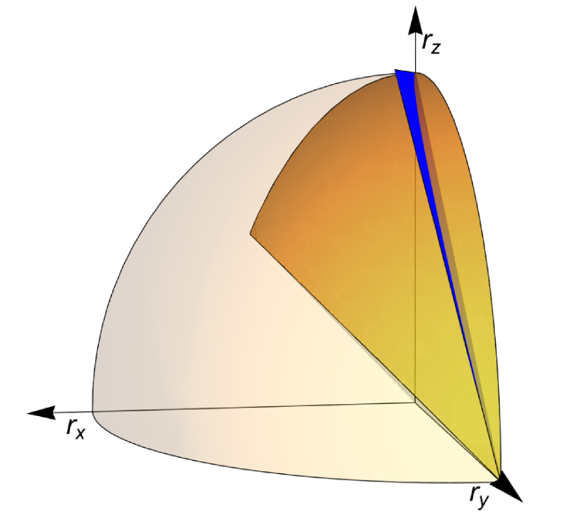
(a)

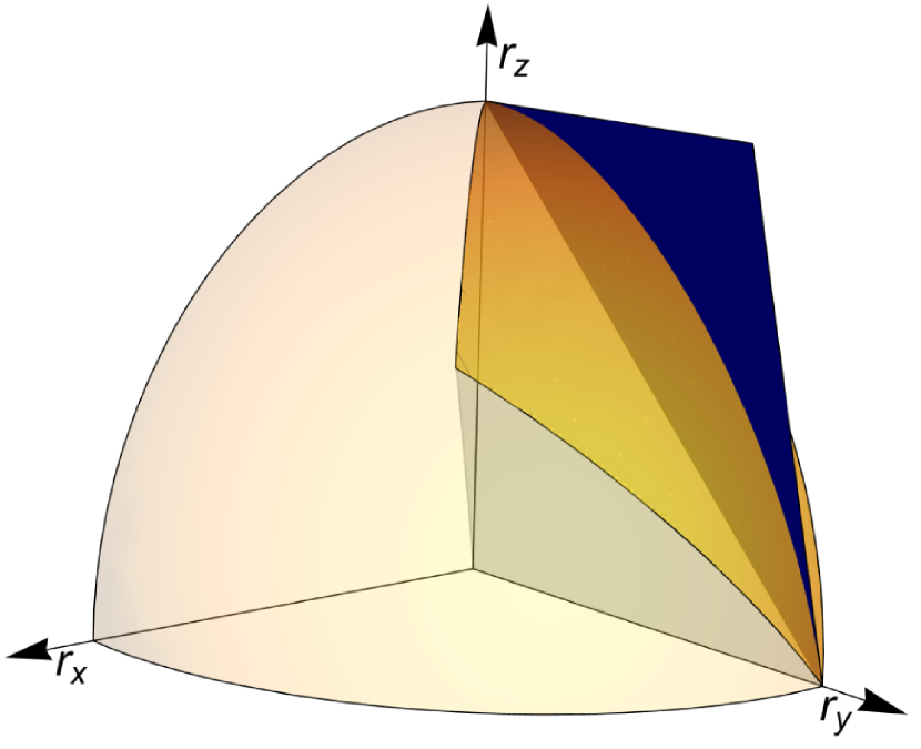
(b)

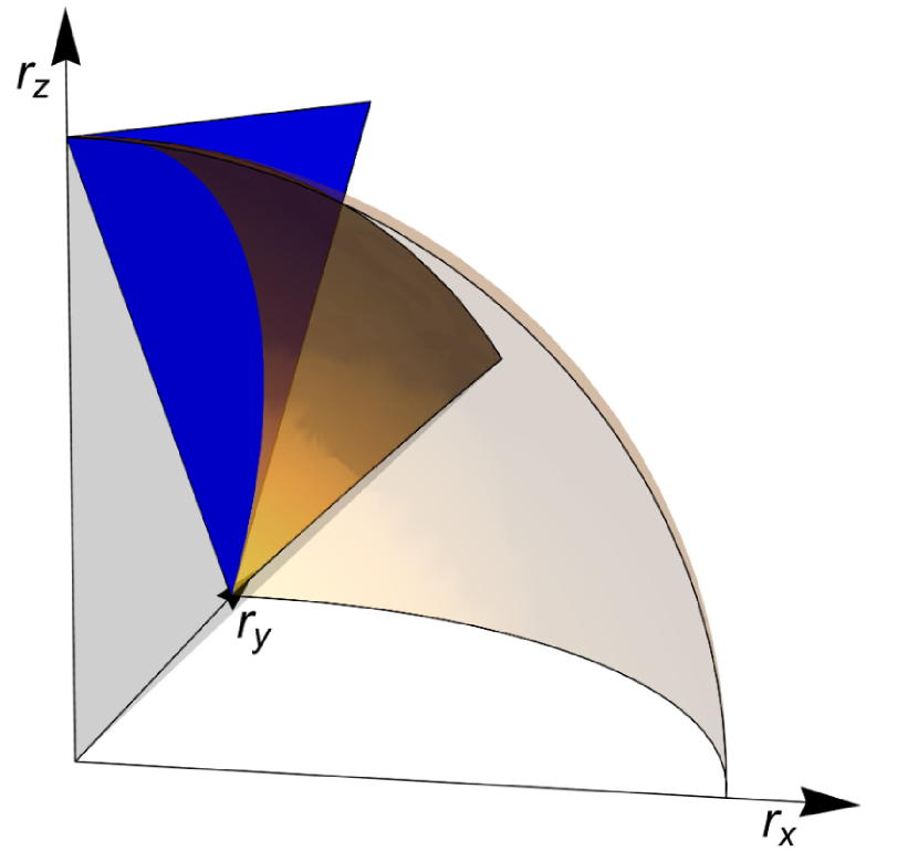
(c)

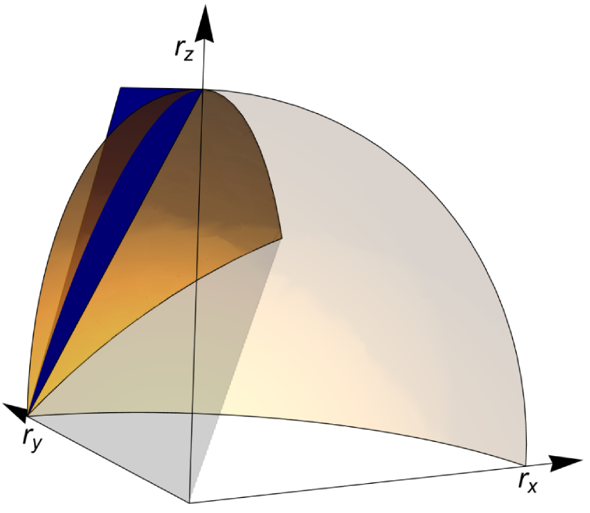
(d)

Figure 3: The figure represents four different angles of the plane $g(\vec{r})=0$ defined in Proposition 6 for the positive octant of the Bloch sphere. The shaded black area is the region $P_{x}$ defined in equation (50). In the region between the plane $g(\vec{r})=0$ and the $z$-$y$ plane of the Bloch sphere it holds $g(\vec{r})\leq 0$. The opposite condition holds on the other side of the plane.

Proof.

We consider the surface with constant $D_{\max}(\rho\|\sigma)$. Here, we think of $\rho$ as a fixed input state. We set $k=\log{D_{\max}(\rho\|\sigma)}$ and we denote the Bloch vectors of $\rho$ and $\sigma$ as $\vec{r}$ and $\vec{s}$, respectively. We also assume that $\rho\in P_{x}$. We define $a(\vec{s})=1-|\vec{s}|^{2}$ and $b(\vec{s})=1-\vec{r}\cdot\vec{s}$ and $d=1-|\vec{r}|^{2}$. Using Lemma 23 we have

$$ka(\vec{s})-b(\vec{s})=\sqrt{b(\vec{s})^{2}-da(\vec{s})}\,.$$ (52)

We then take the square and rearrange the terms to get

$$k^{2}a(\vec{s})-2kb(\vec{s})+d=0\,.$$ (53)

Using the explicit form of the coefficients $a(\vec{s})$ and $b(\vec{s})$ we obtain

$$\left(s_{x}-\frac{r_{x}}{k}\right)^{2}+\left(s_{y}-\frac{r_{y}}{k}\right)^{2}+\left(s_{z}-\frac{r_{z}}{k}\right)^{2}=\left(1-\frac{1}{k}\right)^{2}\,.$$ (54)

The above equation is a sphere with a center that goes to zero and with a radius that goes to $1$ as $k$ grows to infinity. We denote the coordinates of the centers $r_{ki}=r_{i}/k$. To find the smallest $k$ at which the spheres intersect the stabilizer polytope, we first calculate the projection of the points $(r_{kx},r_{ky},r_{kz})$ onto the stabilizer plane $s_{x}+s_{y}+s_{z}=1$. We then compute the distance between the projection and the point and set it equal to the value of the radius. Finally, we then solve for $k$. To find the projection we set

$$(x_{k},y_{k},z_{k})=(r_{kx},r_{ky},r_{kz})+\lambda(1,1,1)\,,$$ (55)

which gives by requiring $x_{k}+y_{k}+z_{k}=1$ the value $\lambda=(1-r_{kx}-r_{ky}-r_{kz})/3$. Hence, the projection is

$$(x_{k},y_{k},z_{k})=\left(\frac{2}{3}r_{kx}+\frac{1}{3}(1-r_{ky}-r_{kz}),\frac{2}{3}r_{ky}+\frac{1}{3}(1-r_{kx}-r_{kz}),\frac{2}{3}r_{kz}+\frac{1}{3}(1-r_{ky}-r_{kx})\right)\,.$$ (56)

By setting the distance between the center and the projection equal to the radius, we obtain the equation

$$1-\frac{1}{k^{*}}=-\frac{1}{\sqrt{3}}(1-r_{k^{*}x}-r_{k^{*}y}-r_{k^{*}z})\,.$$ (57)

The reason for the minus sign when we calculate the square root on the r.h.s. is that, as it is easy to check with the value of $k^{*}$ below, we always have $r_{ky}+r_{kx}+r_{kz}\geq 1$ for any $k\leq k^{*}$ since $r_{x}+r_{y}+r_{z}\geq 1$ for magic states. The above equation gives for $k^{*}=2^{\mathfrak{D}_{\max}(\rho)}$ the value

$$k^{*}=\frac{1}{\sqrt{3}+1}(\sqrt{3}+r_{x}+r_{y}+r_{z})\,.$$ (58)

We now distinguish two cases. The first case is the one for which the projection is inside the Bloch sphere, i.e. $x_{k}^{*}\geq 0$ (note that inside $P_{x}$ we have that $x_{k}$ is always smaller than $y_{k}$ and $z_{k}$). In this case the result above holds since the projection is inside the Bloch sphere. Using the value of $k^{*}$, the condition $x_{k^{*}}\geq 0$ gives

$$r_{x}(2+\sqrt{3})+1-r_{y}-r_{z}\geq 0\,.$$ (59)

The second case is the one for which using the above value of $k^{*}$, the projection onto the plane lies outside the Bloch sphere, i.e. $x_{k}^{*}\leq 0$. In this case, since the optimizer is on the $y$-$z$ plane, we calculate the projection with the stabilizer straight line $s_{z}=1-s_{y}$, $sx=0$. We first construct the plane orthonormal to the line $s_{z}=1-s_{y}$ and find the constant parameter $d$ for which it passes through the point $(r_{kx},r_{ky},r_{kz})$. The equation of the plane is $s_{y}-s_{z}+d=0$ which gives $d=r_{kz}-r_{ky}$. We set $s_{y}=t$ and $s_{z}=1-t$ and substitute in the equation of the plane to find $t=(r_{ky}-r_{kz}+1)/2$ which gives the projection $y_{k}=(r_{ky}-r_{kz}+1)/2$ and $z_{k}=(r_{kz}-r_{ky}+1)/2$ (note that they are positive since each Bloch component is smaller than $1$ and $k\geq 1$). Setting again the distance between the point and the projection equal to the radius, solving the second-order equation, and discarding the negative solution, we find

$$k^{*}=2-r_{y}-r_{z}+\sqrt{2r_{x}^{2}+2(1-r_{y}-r_{z})^{2}}\,.$$ (60)

∎

7.2 Stabilizer fidelity

We now give a closed-form expression of the stabilizer fidelity for single-qubit states.

Proposition 7.

Let $\rho\notin\bar{S}$ be a single-qubit state with Bloch vector $\vec{r}$ in the positive octant. If $\rho\in P_{x}$ then

$$\mathfrak{F}(\rho)=\begin{cases}\frac{1}{6}\left(3+\|\vec{r}\|_{1}+\sqrt{6-2\|\vec{r}\|_{1}^{2}}\right)&\text{if}\quad f(\vec{r})\geq 0\\ \frac{1}{4}\left(2+\|\vec{r}\|_{1}-r_{x}+\sqrt{2(1-r_{x}^{2})-(\|\vec{r}\|_{1}-r_{z})^{2}}\right)&\text{if}\quad f(\vec{r})\leq 0\end{cases}\,,$$ (61)

where $f(\vec{r}):=3-\|\vec{r}\|^{2}_{1}-\sqrt{6-2\|\vec{r}\|_{1}^{2}}(\|\vec{r}\|_{1}-3r_{x})$. For the regions $P_{y}$ and $P_{z}$ the results can be obtained by exchanging $r_{x}\leftrightarrow r_{y}$ and $r_{x}\leftrightarrow r_{z}$, respectively.

We show in Fig. 4 the curved surface $f(\vec{r})=0$.

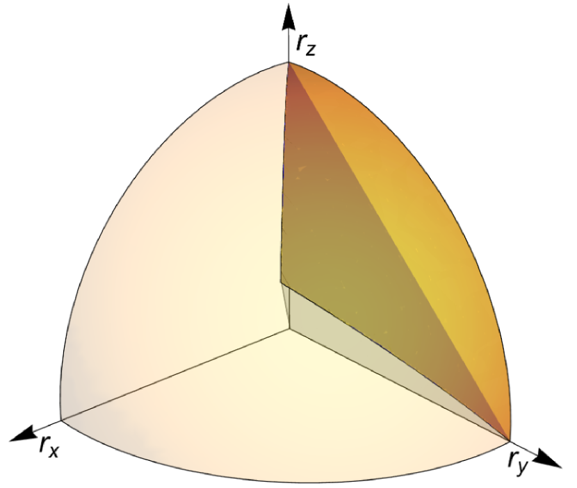
(a)

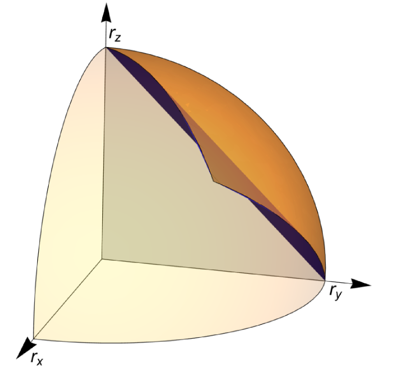
(b)

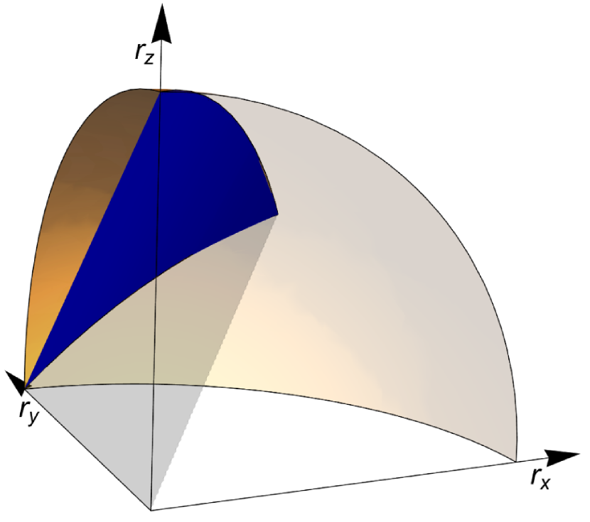
(c)

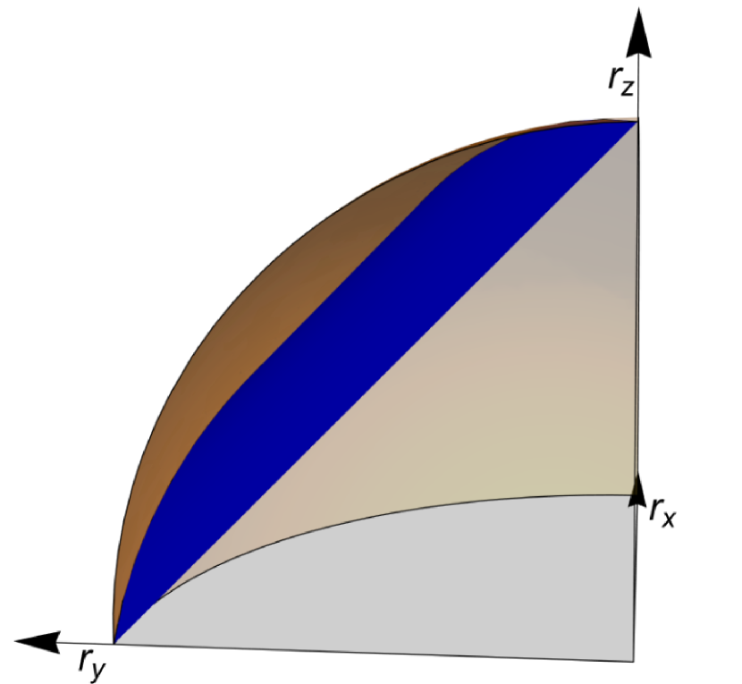
(d)

Figure 4: The figure represents four different angles of the curved surface $f(\vec{r})=0$ defined in Proposition 7 for the positive octant of the Bloch sphere. The shaded black area is the region $P_{x}$ defined in equation (50). In the region closer to the origin it holds $f(\vec{r})\geq 0$. The opposite condition holds on the other side of the curved surface.

Proof.

The fidelity between two qubits $\rho$ and $\sigma$ with Bloch vectors $\vec{r}$ and $\vec{s}$ is [27]

$$F(\rho,\sigma)=\frac{1}{2}\left(1+\vec{r}\cdot\vec{s}+\sqrt{(1-|\vec{r}|^{2})(1-|\vec{s}|^{2})}\right)\,.$$ (62)

We consider the surface with constant $F(\rho,\sigma)$. We set $k=2F(\rho,\sigma)-1$. We define $h(\vec{s})=\vec{r}\cdot\vec{s}$, $m(\vec{s})=1-|\vec{s}|^{2}$ and $p=1-|\vec{r}|^{2}$. Using the explicit form of the fidelity we obtain

$$\frac{k-h(\vec{s})}{\sqrt{p}}=\sqrt{m(\vec{s})}\,.$$ (63)

We then take the square and rearrange the terms and use the explicit form of the coefficients $h(\vec{s})$ and $m(\vec{s})$ to get

$$s_{x}^{2}(r_{x}^{2}+p)+s_{y}^{2}(r_{y}^{2}+p)+s_{z}^{2}(r_{z}^{2}+p)$$ (64)

$$\quad+2s_{x}s_{y}r_{x}r_{y}+2s_{x}s_{z}r_{x}r_{z}+2s_{y}s_{z}r_{y}r_{z}-2ks_{x}r_{x}-2ks_{y}r_{y}-2kr_{z}s_{z}+k^{2}-p=0\,.$$ (65)

The above equation is a rotated and shifted ellipsoid. To calculate the value of the stabilizer fidelity we consider the intersection with the stabilizer plane $s_{x}+s_{y}+s_{z}=1$ and calculate the value of $k$ for which the ellipsoid intersects the plane in exactly one point. The intersection gives the equation

$$as_{x}^{2}+2bs_{x}s_{y}+cs_{y}^{2}+2ds_{x}+2fs_{y}+g=0\,,$$ (66)

where

$$a=(r_{x}-r_{z})^{2}+2p\,,$$ (67)

$$b=r_{x}r_{y}-r_{x}r_{z}-r_{y}r_{z}+r_{z}^{2}+p\,,$$ (68)

$$c=(r_{y}-r_{z})^{2}+2p\,,$$ (69)

$$d=-r_{z}^{2}-p+r_{x}r_{z}-kr_{x}+kr_{z}\,,$$ (70)

$$f=-r_{z}^{2}-p+r_{y}r_{z}-kr_{y}+kr_{z}\,,$$ (71)

$$g=(k-r_{z})^{2}\,,$$ (72)

which is an equation of an ellipse. From standard geometry analysis, it follows that the center of the ellipse is given by $(x_{k},y_{k})=(b^{2}-ac)^{-1}(cd-bf,af-bd)$. Moreover, the semi-axis of the ellipse are zero when $af^{2}+cd^{2}+gb^{2}-2bdf-acg=0$. A straightforward but lengthy calculation shows that this is the case when

$$k^{*}=\frac{1}{3}(\|\vec{r}\|_{1}+\sqrt{6-2\|\vec{r}\|_{1}^{2}})\,.$$ (73)

We now distinguish two cases. The first case is the one for which the projection is inside the Bloch sphere, i.e. $x_{k}^{*}\geq 0$. A calculation reveals that since $\rho\in P_{x}$ it holds that $x_{k}\leq y_{k}$. Using the value of $k^{*}$, the condition $x_{k}^{*}\geq 0$ gives

$$3-\|\vec{r}\|^{2}_{1}-\sqrt{6-2\|\vec{r}\|_{1}^{2}}(\|\vec{r}\|_{1}-3r_{x})\geq 0\,.$$ (74)

The second case is the one for which using the above value of $k^{*}$, the projection onto the plane lies outside the Bloch sphere, i.e. $x_{k}^{*}\leq 0$. In this case, since the optimizer is on the $y$-$z$ plane, we calculate the intersection with the stabilizer straight line $s_{z}=1-s_{y}$, $s_{x}=0$. Hence, we need to solve the equation

$$s_{y}^{2}(r_{y}^{2}+p)+(1-s_{y})^{2}(r_{z}^{2}+p)+2s_{y}(1-s_{y})r_{y}r_{z}-2s_{y}kr_{y}-2(1-s_{y})kr_{z}+k^{2}-p=0\,.$$ (75)

It is easy to check that the above equation has only one allowed solution for

$$k^{*}=\frac{1}{2}\left(r_{y}+r_{z}+\sqrt{2-2r_{x}^{2}-(r_{y}+r_{z})^{2}}\right)\,.$$ (76)

∎

8 Examples of two and three-qubit states belonging to the additivity classes and their computation

In this section, we show that for some specific states, the optimizer of any monotone based on an $\alpha$-$z$ Rényi divergence commutes with the state itself.

In some cases which involve pure states subject to depolarized noise $\rho=\Delta_{p}(\ket{\psi}\!\!\bra{\psi})$, the optimizer can be inferred from the knowledge of the solution of the related linear optimization $\mathfrak{F}_{0}(\ket{\psi}\!\!\bra{\psi})$. This is typically the case when $\outerproduct{\psi}{\psi}$ has some symmetry.

Lemma 8.

Let $(\alpha,z)\in\mathcal{D}$ and let $\rho$ be a quantum state of dimension $d$ such that $\rho=\Delta_{p}(\ket{\psi}\!\!\bra{\psi})\notin\bar{S}$ for some $p\geq 0$ and a pure state $\ket{\psi}\!\!\bra{\psi}$. If $\tau=\Delta_{t}(\ket{\psi}\!\!\bra{\psi})\in\bar{S}$ for $t=(d\mathfrak{F}_{0}(\ket{\psi}\!\!\bra{\psi})-1)/(d-1)$, then we have that $\tau\in\operatorname*{arg\,min}_{\sigma\in\bar{S}}D_{\alpha,z}(\rho\|\sigma)$.

Proof.

We need to check that the state $\tau=\Delta_{t}(\ket{\psi}\!\!\bra{\psi})$ satisfies the condition of Corollary 18

$$\max\limits_{\sigma\in\bar{S}}\Tr(\sigma\rho^{\alpha}\tau^{-\alpha})=\Tr(\rho^{\alpha}\tau^{1-\alpha})\,.$$ (77)

If we plug in the explicit form of $\tau$ and $\rho$, we get the condition

$$(a-b)\mathfrak{F}_{0}(\ket{\psi}\!\!\bra{\psi})+b=a^{\prime}-b^{\prime}+db^{\prime}\,,$$ (78)

where

$$a=\left(\frac{1+(d-1)p}{1+(d-1)t}\right)^{\alpha},\quad b=\left(\frac{1-p}{1-t}\right)^{\alpha},\quad a^{\prime}=\frac{1-t}{d}a+at,\quad b^{\prime}=\frac{1-t}{d}b\,.$$ (79)

Hence, the condition is equivalent to

$$(a-b)\left(\mathfrak{F}_{0}(\ket{\psi}\!\!\bra{\psi})-\frac{1-t}{d}-t\right)=0\,.$$ (80)

Since $a>b$ because we assume $\rho$ is magic and hence $p>t$, the above product is zero only if $t=(d\mathfrak{F}_{0}(\ket{\psi}\!\!\bra{\psi})-1)/(d-1)$ which proves the theorem. ∎

We point out that the previous lemma can be applied only to specific states since for general states $\tau=\Delta_{t}(\ket{\psi}\!\!\bra{\psi})\notin\bar{S}$ for $t=(d\mathfrak{F}_{0}(\ket{\psi}\!\!\bra{\psi})-1)/(d-1)$. We give a few examples below. We calculate the value of the $\alpha$-$z$ Rényi relative entropies of magic for all the values of the parameters. As discussed in Section 2, the value of the stabilizer fidelity, the relative entropy of magic, and the generalized log-robustness of magic can be obtained by taking the limits $\alpha\rightarrow 1/2$, $\alpha\rightarrow 1$ and $\alpha\rightarrow\infty$, respectively.

8.1 T, H and F states

The $T,H$, and $F$ states are the pure states located in the symmetry axes of the stabilizer octahedron in the positive octant of the Bloch sphere. They are defined as

$$\outerproduct{H}{H}=\frac{1}{2}\left(1+\frac{X+Z}{\sqrt{2}}\right)\,,\quad\outerproduct{T}{T}=\frac{1}{2}\left(1+\frac{X+Y}{\sqrt{2}}\right)\,,\quad\outerproduct{F}{F}=\frac{1}{2}\left(1+\frac{X+Y+Z}{\sqrt{3}}\right)\,.$$ (81)

We proved in Section 7 that for the stabilizer fidelity and the generalized robustness, the optimizer of the latter states lies at the intersection between the line joining the states with the center of the Bloch sphere and the stabilizer octahedron. This is true even in the presence of depolarizing noise. As a result, for the states belonging to the symmetry axes of the octahedron, the optimizer commutes with the state itself. Here, we extend the latter result to include all the $\alpha$-$z$ Rényi relative entropy of magic, which notably, includes the relative entropy of magic. These states are the only single-qubit states that commute with their optimizer.

Proposition 9.

Let $p\geq 1/\sqrt{2}$. We have

$$\mathfrak{D}_{\alpha,z}(\Delta_{p}(\outerproduct{H}{H}))=\mathfrak{D}_{\alpha,z}(\Delta_{p}(\outerproduct{T}{T}))$$ (82)

$$\quad\qquad\qquad\qquad\quad=\frac{1}{\alpha-1}\log\left(\frac{\left(1+p\right)^{\alpha}}{2}\left(1+\frac{1}{\sqrt{2}}\right)^{1-\alpha}+\frac{\left(1-p\right)^{\alpha}}{2}\left(1-\frac{1}{\sqrt{2}}\right)^{1-\alpha}\right)\,.$$ (83)

Let $p\geq 1/\sqrt{3}$. We have

$$\mathfrak{D}_{\alpha,z}(\Delta_{p}(\outerproduct{F}{F}))=\frac{1}{\alpha-1}\log\left(\frac{\left(1+p\right)^{\alpha}}{2}\left(1+\frac{1}{\sqrt{3}}\right)^{1-\alpha}+\frac{\left(1-p\right)^{\alpha}}{2}\left(1-\frac{1}{\sqrt{3}}\right)^{1-\alpha}\right)\,.$$ (84)

Moreover, for the above states, the optimizer commutes with the input state.

Proof.

Since the pure single-qubit stabilizer states are the eigenvectors of the Pauli matrices, by explicit computation, it is easy to prove that for a single-qubit state $\rho$ it holds $\mathfrak{F}_{0}(\rho)=(1+\max_{i}|r_{i}|)/2$. Here, we denoted with $\vec{r}$ the Bloch vector of $\rho$. Hence, we have that

$$\mathfrak{F}_{0}(\outerproduct{H}{H})=\mathfrak{F}_{0}(\outerproduct{T}{T})=\frac{1}{2}\left(1+\frac{1}{\sqrt{2}}\right)\,\quad\mathfrak{F}_{0}(\outerproduct{F}{F})=\frac{1}{2}\left(1+\frac{1}{\sqrt{3}}\right)\,.$$ (85)

Setting $t_{\outerproduct{\psi}{\psi}}=(d\mathfrak{F}_{0}(\ket{\psi}\!\!\bra{\psi})-1)/(d-1)$, it is straightforward to prove that for these specific states, $\Delta_{t_{\outerproduct{\psi}{\psi}}}(\outerproduct{\psi}{\psi})$ is a stabilizer state. Here, we set $\psi=H,T$ and $F$. Hence, we can apply Lemma 8. The proposition follows by explicit computation. ∎

Outside the above ranges of $p$, the input state is a stabilizer state and hence the monotones evaluate to zero.

8.2 Toffoli state

The Toffoli state is

$$\ket{\text{Toffoli}}=\frac{\ket{000}+\ket{100}+\ket{010}+\ket{111}}{2}\,.$$ (86)

The Toffoli state is Clifford equivalent to the $\ket{CCZ}$ state [24]. We now show that for the Toffoli state, we have that $\mathfrak{F}_{0}(\ket{\text{Toffoli}}\!\!\bra{\text{Toffoli}})=9/16$. Note first that the maximization is always achieved by a pure stabilizer state due to the linearity of the trace.

Any $n$-qubit pure stabilizer state is a simultaneous $+1$ or $-1$ eigenstate of $n$ commuting independent Pauli operators and their arbitrary product ($2^{n}$ Pauli operators in total). This means that, for an arbitrary $n$-qubit pure stabilizer state $\ket{\phi}$, there exists a set of commuting $n$-qubit independent Pauli operators $\{P_{k}\}_{k=1}^{n}$ and eigenvalues $\lambda_{k}\in\{+1,-1\}$ such that

$$\outerproduct{\phi}{\phi}=\prod_{k=1}^{n}\frac{\mathbb{I}+{\lambda_{k}}P_{k}}{2}=\frac{1}{2^{n}}\sum_{Q\in\mathcal{S}}\lambda_{Q}Q\,,$$ (87)

where $\mathcal{S}$ is the set of Pauli operators generated by $\{P_{i}\}_{i=1}^{n}$, which has size $2^{n}$, and $\lambda_{Q}\in\{+1,-1\}$ that satisfies $(-1)^{k}\lambda_{Q_{1}}\lambda_{Q_{2}}=\lambda_{Q}$ for $Q_{1},Q_{2}\in\mathcal{S}$ such that $Q_{1}Q_{2}=(-1)^{k}Q,\ k\in\{0,1\}$. We expand $\outerproduct{\text{Toffoli}}{\text{Toffoli}}=2^{-n}\sum_{Q=1}^{4^{n}}r_{Q}Q$ in the Pauli basis. Here, $r_{Q}=\Tr(Q\outerproduct{\text{Toffoli}}{\text{Toffoli}})$ and since the Toffoli state is a three-qubit state, we have that $n=3$. Noting that every non-identity Pauli operator is traceless, the terms that survive in $|\innerproduct{\phi}{\text{Toffoli}}|^{2}$ are the ones with a Pauli in $\mathcal{S}$. It is a straightforward calculation to check that the coefficients $r_{Q}$ of the Toffoli state in the Pauli basis are at most $1/2$. This gives for any pure stabilizer state $\ket{\phi}$

$$|\innerproduct{\phi}{\text{Toffoli}}|^{2}=\frac{1}{8}\sum_{Q\in\mathcal{S}}\lambda_{Q}r_{Q}\leq\frac{1}{8}\left(1+\frac{7}{2}\right)=\frac{9}{16}\,.$$ (88)

An easy calculation reveals that the above bound is achieved by the stabilizer state $\ket{\phi}$ with generators $\{\mathds{1}\otimes\mathds{1}\otimes\mathds{1},\mathds{1}\otimes\mathds{1}\otimes X,\mathds{1}\otimes X\otimes\mathds{1},Z\otimes\mathds{1}\otimes\mathds{1}\}$. The latter result has been obtained in [6].

From Lemma 8 we get the stabilizer state $\tau=\frac{1}{2}\ket{\text{Toffoli}}\!\!\bra{\text{Toffoli}}+\frac{1}{2}\frac{\mathds{I}}{8}$. By direct computation, we obtain

Proposition 10.

Let $p\geq 1/2$. We have

$$\mathfrak{D}_{\alpha,z}(\Delta_{p}(\outerproduct{\textup{Toffoli}}{\textup{Toffoli}}))=\frac{1}{\alpha-1}\log\left(2^{\alpha-4}(7(1-p)^{\alpha}+9^{1-\alpha}(1+7p)^{\alpha})\right)\,.$$ (89)

Moreover, the optimizer is a depolarized Toffoli state.

8.3 Hoggar state

The Hoggar state is defined as [20]

$$\ket{\text{Hog}}=\frac{(1+i)\ket{000}+\ket{010}+\ket{110}+\ket{100}+\ket{101}}{\sqrt{6}}\,.$$ (90)

For the Hoggar state we have that $\mathfrak{F}_{0}(\ket{\text{Hog}}\!\!\bra{\text{Hog}})=2^{-\mathfrak{D}_{\min}(\ket{\text{Hog}}\!\!\bra{\text{Hog}})}=5/12$ [42]. Using the previous lemma we get the stabilizer optimizer $\tau=\frac{1}{3}\ket{\text{Hog}}\!\!\bra{\text{Hog}}+\frac{2}{3}\frac{\mathds{I}}{8}$.

Proposition 11.

Let $p\geq 1/3$. We have

$$\mathfrak{D}_{\alpha,z}(\Delta_{p}(\outerproduct{\textup{Hog}}{\textup{Hog}}))=\frac{1}{\alpha-1}\log\left(\frac{3^{\alpha-1}}{2^{\alpha+2}}(7(1-p)^{\alpha}+5^{1-\alpha}(1+7p)^{\alpha})\right)\,.$$ (91)

Moreover, the optimizer is a depolarized Hoggar state.

8.4 CS state

The $\ket{CS}=CS|+\rangle^{\otimes 2}$ reads

$$\ket{CS}=\frac{1}{2}(\ket{00}+\ket{01}+\ket{10}+i\ket{11})\,.$$ (92)

It is a straightforward calculation to check that the coefficients $r_{Q}$ of the CS-state in the Pauli basis are at most $1/2$. This gives for any pure stabilizer state $\ket{\phi}$

$$|\innerproduct{\phi}{CS}|^{2}=\frac{1}{4}\sum_{Q\in\mathcal{S}}\lambda_{Q}r_{Q}\leq\frac{1}{4}\left(1+\frac{3}{2}\right)=\frac{5}{8}\,.$$ (93)

An easy calculation reveals that the above bound is achieved by the stabilizer state $\ket{\phi}$ with generators $\{\mathds{1}\otimes\mathds{1},-\mathds{1}\otimes Y,X\otimes\mathds{1}\}$.

From Lemma 8 we get the stabilizer state $\tau=\frac{1}{2}\ket{CS}\!\!\bra{CS}+\frac{1}{2}\frac{\mathds{I}}{4}$. By direct calculation, we get

Proposition 12.

Let $p\geq 1/2$. We have

$$\mathfrak{D}_{\alpha,z}(\Delta_{p}(\outerproduct{\text{CS}}{\text{CS}}))=\frac{1}{\alpha-1}\log\left(2^{\alpha-3}(3(1-p)^{\alpha}+5^{1-\alpha}(1+3p)^{\alpha})\right)\,.$$ (94)

Moreover, the optimizer is a depolarized CS state.

9 No additivity for any monotone based on a quantum relative entropy for general odd-dimensional states

In [47] the authors provided a counterexample to the additivity of the relative entropy of magic for qutrit states. We now show that the latter statement can be generalized to include any monotone based on a quantum relative entropy. We call a monotone based on a quantum relative entropy any monotone of the form $\min_{\sigma\in\mathcal{F}}\mathbb{D}(\rho\|\sigma)$ where $\mathbb{D}$ is a quantum relative entropy [17]. We have

Proposition 13.

Any monotone based on a quantum divergence is not additive for two pure qutrit strange states.

Proof.

The relative entropy is not additive for the tensor product of two qutrit strange states [47]. Moreover, the value of the relative entropy of magic is equal for both strange states and tensor products of strange states to the value of the $\mathfrak{D}_{\min}$ and $\mathfrak{D}_{\max}$ [42, Proposition 14]. Since any monotone based on a quantum relative entropy is contained between $\mathfrak{D}_{\min}$ and $\mathfrak{D}_{\max}$ [17], it follows that any monotone based on a quantum divergence is not additive for general states. ∎

Note that, since the counterexample involves pure states, it extends to any monotone defined through convex-roof construction.

10 A possible direction to prove the additivity of the $\alpha$-$z$ Rényi relative entropies of magic in the range $|(1-\alpha)|/z=1$ for all two and three-qubit states

In this section, we propose a direction to prove additivity for all two and three-qubit states for the $\alpha$-$z$ Rényi relative entropies of magic in the range $|(1-\alpha)|/z=1$. To do so, we generalize to mixed states the stabilizer-aligned condition introduced in [6, Definition 9] for pure states.

The 2-norm of a matrix $A$ is defined as $\|A\|_{2}:=(\Tr(A^{\dagger}A))^{\frac{1}{2}}$. We call $S_{n,m}$ the set of rank-$2^{m}$ stabilizer projectors on $n$ qubits.

Definition 14.

For any n-qubit state $\rho$, define

$$\mathfrak{F}_{m}(\rho)=2^{-m/2}\max\limits_{\Pi_{m}\in S_{n,m}}\|\Pi_{m}\rho\Pi_{m}\|_{2}\qquad m=0,..,n\,.$$ (95)

We say that $\rho$ is stabilizer-aligned if $\mathfrak{F}_{m}(\rho)\leq\mathfrak{F}_{0}(\rho)$ for all $m$.

Lemma 15.

Let $\rho_{1}$ and $\rho_{2}$ be stabilizer-aligned. Then, it holds that $\mathfrak{F}_{0}(\rho_{1}\otimes\rho_{2})=\mathfrak{F}_{0}(\rho_{1})\mathfrak{F}_{0}(\rho_{2})$.

Proof.

Since $\mathfrak{F}_{0}$ is super-multiplicative, we need to show that for two stabilizer-aligned states, $\mathfrak{F}_{0}(\rho_{1}\otimes\rho_{2})\leq\mathfrak{F}_{0}(\rho_{1})\mathfrak{F}_{0}(\rho_{2})$. We use that for a bipartite stabilizer state $|\phi\rangle$, there exists a local Clifford $U_{A}\otimes U_{B}$ and $d\geq 0$ such that $U_{A}\otimes U_{B}\ket{\phi}=\ket{\omega_{d}}=2^{-d/2}\sum_{\delta=1}^{2^{d}}\ket{\delta}\ket{\delta}$ [7, Theorem 5]. Since local Clifford unitary does not change $\mathfrak{F}_{0}$, we absorb the unitaries $U_{A}$ and $U_{B}$ into the states $\rho_{1}$ and $\rho_{2}$. We use the spectral decomposition into (not normalized) orthogonal states $\rho_{1}=\sum_{i}\outerproduct{\phi_{i}}{\phi_{i}}$ and $\rho_{2}=\sum_{j}\outerproduct{\psi_{j}}{\psi_{j}}$. We have

$$\mathfrak{F}_{0}(\rho_{1}\otimes\rho_{2})=\sum_{ij}\innerproduct{\omega_{d}}{\phi_{i}\psi_{j}}\innerproduct{\phi_{i}\psi_{j}}{\omega_{d}}=\sum_{ij}|\innerproduct{\phi_{i}\psi_{j}}{\omega_{d}}|^{2}=2^{-d}\sum_{ij}\left|\sum_{\delta=1}^{2^{d}}\innerproduct{\phi_{i}}{\delta}\innerproduct{\psi_{j}}{\delta}\right|^{2}\,.$$ (96)

We now define the matrices

$$\Phi=\begin{pmatrix}\innerproduct{\phi_{1}}{1}&...&\innerproduct{\phi_{2^{n}}}{1}\\ \vdots&...&\vdots\\ \innerproduct{\phi_{1}}{2^{d}}&...&\innerproduct{\phi_{2^{n}}}{2^{d}}\end{pmatrix}\,,\qquad\Psi=\begin{pmatrix}\innerproduct{\psi_{1}}{1}&...&\innerproduct{\psi_{2^{n}}}{1}\\ \vdots&...&\vdots\\ \innerproduct{\psi_{1}}{2^{d}}&...&\innerproduct{\psi_{2^{n}}}{2^{d}}\end{pmatrix}\,.$$ (97)

We note that $\mathfrak{F}_{0}(\rho_{1}\otimes\rho_{2})=2^{-d}\|\Phi^{T}\Psi\|_{2}^{2}$. We now use a variation of Holder’s inequality [4, Exercise IV.2.7] which states $\|\Phi^{T}\Psi\|_{2}\leq\|\Phi^{T}\|_{4}\|\Psi\|_{4}$. An explicit calculation shows that $\|\Phi^{T}\|_{4}=(\Tr(\Phi^{\dagger}\Phi\Phi^{\dagger}\Phi))^{\frac{1}{4}}=\Tr(\rho_{1}\Pi_{d}\rho_{1}\Pi_{d})^{\frac{1}{4}}$ and, analogously $\|\Psi\|_{4}=\Tr(\rho_{2}\Pi_{d}\rho_{2}\Pi_{d})^{\frac{1}{4}}$ where $\Pi_{d}=\sum_{\delta=1}^{2^{d}}\outerproduct{\delta}{\delta}$. If both states are stabilizer-aligned, we therefore get

$$\mathfrak{F}_{0}(\rho_{1}\otimes\rho_{2}) =2^{-d}\|\Phi^{T}\Psi\|_{2}^{2}$$ (98)

$$\leq 2^{-d}\Tr(\rho_{1}\Pi_{d}\rho_{1}\Pi_{d})^{\frac{1}{2}}\Tr(\rho_{2}\Pi_{d}\rho_{2}\Pi_{d})^{\frac{1}{2}}$$ (99)

$$\leq\mathfrak{F}_{0}(\rho_{1})\mathfrak{F}_{0}(\rho_{2})\,,$$ (100)

which proves the lemma. ∎

We now show that single-qubit states are stabilizer-aligned.

Lemma 16.

All single-qubit states are stabilizer-aligned.

Proof.

We can write any qubit in the Bloch representation $\rho=(1/2)(1+\sum_{p}c_{p}P)$, where the sum runs over the Pauli matrices. It is easy to check that $\mathfrak{F}_{1}(\rho)=2^{-1/2}\sqrt{\Tr(\rho^{2})}=(1/2)\sqrt{(1+\sum_{p}c_{p}^{2})}$ since the only projector of rank-two is the identity. Moreover, $\mathfrak{F}_{0}(\rho)=(1/2)(1+|c_{p^{*}}|)$, where $c_{p^{*}}=\max_{p}c_{p}$. The condition $\mathfrak{F}_{0}(\rho)\geq\mathfrak{F}_{1}(\rho)$ then reads $c_{p^{*}}^{2}+2|c_{p^{*}}|\geq\sum_{p}c_{p}^{2}$. Using that $|c_{p^{*}}|\leq 1$ and that the maximum is greater than the average, we get $|c_{p^{*}}|\geq c_{p^{*}}^{2}\geq\sum_{p}c_{p}^{2}/3$. It then follows that $c_{p^{*}}^{2}+2|c_{p^{*}}|\geq(1/3+2/3)\sum_{p}c_{p}^{2}=\sum_{p}c_{p}^{2}$ which proves the inequality. ∎

Following similar arguments that lead to Theorem 2, the above results imply the additivity of the $\alpha$-$z$ Rényi relative entropies of magic in the range $|(1-\alpha)|/z=1$ for two single-qubit states. It is an open problem whether the proof of Lemma 15 can be generalized to products of more than two stabilizer-aligned states. Moreover, it is still an open question whether all the two and three-qubit states are stabilizer-aligned according to the above definition. If these two questions could be resolved in the affirmative, additivity of the $\alpha$-$z$ Rényi relative entropies of magic in the range $|(1-\alpha)|/z=1$ would follow for any number of any two and three-qubit states.

Appendices

A Necessary and sufficient conditions for the optimizer

In this appendix, we review the necessary and sufficient conditions for the optimizer(s) of the $\alpha$-$z$ Rényi relative entropies of magic derived in [37]. The results are very general and hold for any resource theory. In this manuscript, we consider $\mathcal{F}=\bar{S}$. Let $\rho,\tau\in\mathcal{S}(A)$. We define

$$\Xi_{\alpha,z}(\rho,\tau):=\begin{dcases}\chi_{\alpha,1-\alpha}(\rho,\tau)&\textup{if}\;z=1-\alpha\\ \tau^{-1}\chi_{\alpha,\alpha-1}(\rho,\tau)\tau^{-1}&\textup{if}\;z=\alpha-1\\ K_{\alpha,z}\int_{0}^{\infty}\frac{\chi_{\alpha,z}(\rho,\tau)}{(\tau+t)^{2}}t^{\frac{1-\alpha}{z}}\mathrm{d}t&\textup{if}\;|(1-\alpha)/z|\neq 1\end{dcases}\,,$$ (101)

where $K_{\alpha,z}:=\operatorname{sinc}\left(\pi\frac{{1-\alpha}}{z}\right)$ is a positive constant and we defined the positive operator $\chi_{\alpha,z}(\rho,\tau):=\rho^{\frac{\alpha}{2z}}(\rho^{\frac{\alpha}{2z}}\tau^{\frac{1-\alpha}{z}}\rho^{\frac{\alpha}{2z}})^{z-1}\rho^{\frac{\alpha}{2z}}$.

Moreover, we define

$$S_{\alpha,z}(\rho)=\begin{cases}\left\{\sigma\in\mathcal{S}(A):\operatorname{supp}(\rho)=\operatorname{supp}\!\left(\Pi(\rho)\sigma\Pi(\rho)\right)\right\}&\textup{if}\;(1-\alpha)/z=1\\ \left\{\sigma\in\mathcal{S}(A):\operatorname{supp}(\rho)\subseteq\operatorname{supp}(\sigma)\right\}&\textup{otherwise}\end{cases}\,,$$ (102)

We have the following result [37]

Theorem 17.

Let $\rho$ be a quantum state and $(\alpha,z)\in\mathcal{D}$. Then $\tau\in\operatorname*{arg\,min}_{\sigma\in\mathcal{F}}D_{\alpha,z}(\rho\|\sigma)$ if and only if $\tau\in S_{\alpha,z}(\rho)$ and $\textup{Tr}(\sigma\,\Xi_{\alpha,z}(\rho,\tau))\leq Q_{\alpha,z}(\rho\|\tau)$ for all $\sigma\in\mathcal{F}$.

In this case, the above theorem considerably simplifies.

Corollary 18.

Let $\rho$ be a quantum state and $(\alpha,z)\in\mathcal{D}$. Then, a state $\tau$ satisfying $[\rho,\tau]=0$ belongs to the set $\tau\in\operatorname*{arg\,min}_{\sigma\in\mathcal{F}}D_{\alpha,z}(\rho\|\sigma)$ if and only if $\operatorname{supp}(\rho)\subseteq\operatorname{supp}(\tau)$ and $\textup{Tr}(\sigma\Xi_{\alpha}(\rho,\tau))\leq Q_{\alpha}(\rho\|\tau)$ for all $\sigma\in\mathcal{F}$ where $\Xi_{\alpha}(\rho,\tau)=\rho^{\alpha}\tau^{-\alpha}$ and $Q_{\alpha}(\rho\|\tau)=\textup{Tr}(\rho^{\alpha}\tau^{1-\alpha})$.

B Properties of the resource monotones based on the $\alpha$-$z$ Rényi relative entropies

In this Appendix, we discuss some of the properties satisfied by the monotones based on the $\alpha$-$z$ Rényi relative entropies. These properties have already been discussed extensively in entanglement theory [44, 49] for some specific values of the parameters. Moreover, the generalized robustness case has been discussed in [32] for any convex resource theories. Here, we give a more general proof that holds for any convex resource theory and all the values of the parameters $(\alpha,z)\in\mathcal{D}$. In this case, the same definitions given in the main text hold with the set of stabilizer states $\bar{S}$ replaced by a general convex set of free states $\mathcal{F}$. We first prove that the monotones are convex or concave, depending on the value of the parameter.

Lemma 19.

Let $(\alpha,z)\in\mathcal{D}$, $\{\rho_{i}\}_{i}$ a set of states and $\{p_{i}\}_{i}$ a set of weights, i.e. $p_{i}\geq 0$ and $\sum_{i}p_{i}=1$. Then, we have

$$\mathcal{Q}_{\alpha,z}^{\frac{1}{\alpha}}\Big{(}\sum\nolimits_{i}p_{i}\rho_{i}\Big{)}\geq\sum\nolimits_{i}p_{i}\mathcal{Q}_{\alpha,z}^{\frac{1}{\alpha}}(\rho_{i})\,,\quad\quad\alpha<1$$ (103)

$$\mathcal{Q}_{\alpha,z}^{\frac{1}{\alpha}}\Big{(}\sum\nolimits_{i}p_{i}\rho_{i}\Big{)}\leq\sum\nolimits_{i}p_{i}\mathcal{Q}_{\alpha,z}^{\frac{1}{\alpha}}(\rho_{i})\,,\quad\quad\alpha>1$$ (104)

$$\mathfrak{D}\Big{(}\sum\nolimits_{i}p_{i}\rho_{i}\Big{)}\leq\sum\nolimits_{i}p_{i}\mathfrak{D}(\rho_{i})\,.$$ (105)

Proof.

We first consider case $\alpha>1$. We denote with $\tau_{i}$ an optimizer of $\rho_{i}$, i.e a state such that $\mathcal{Q}_{\alpha,z}(\rho_{i})=Q_{\alpha,z}(\rho_{i}\|\tau_{i})$. We define the probability vector

$$t_{k}=\frac{p_{k}Q^{\frac{1}{\alpha}}_{\alpha,z}(\rho_{k}\|\tau_{k})}{\sum_{i}p_{i}Q^{\frac{1}{\alpha}}_{\alpha,z}(\rho_{i}\|\tau_{i})}\,.$$ (106)

We then have

$$\mathcal{Q}_{\alpha,z}\Big{(}\sum\nolimits_{i}p_{i}\rho_{i}\Big{)} \leq Q_{\alpha,z}\left(\sum\nolimits_{i}p_{i}\rho_{i}\middle\|\sum\nolimits_{i}t_{i}\tau_{i}\right)$$ (107)

$$\leq Q_{\alpha,z}\left(\sum\nolimits_{i}p_{i}\rho_{i}\otimes\outerproduct{i}{i}\middle\|\sum\nolimits_{i}t_{i}\tau_{i}\otimes\outerproduct{i}{i}\right)$$ (108)

$$=\sum\nolimits_{i}p_{i}^{\alpha}t_{i}^{1-\alpha}Q_{\alpha,z}\left(\rho_{i}\middle\|\tau_{i}\right)$$ (109)

$$=\left(\sum\nolimits_{i}p_{i}\mathcal{Q}_{\alpha,z}^{\frac{1}{\alpha}}(\rho_{i})\right)^{\alpha}\,.$$ (110)

In the first inequality (107) we used that a mixture of free states is free and (108) follows for the DPI under partial trace. The last two steps follow by direct computation. We case $\alpha<1$ is similar and the result for the relative entropy follows from joint convexity of the relative entropy (see, e.g., [3]). ∎

We now discuss the strong monotonicity property (see e.g. [44, 39, 3, 32]). An instrument is a collection of complete positive trace-nonincreasing operations $\{\Phi_{i}\}$ such that the overall transformation $\sum_{i}\Phi_{i}$ is trace-preserving. We say that $\{\Phi_{i}\}$ is a free probabilistic instrument if each operation maps a free state into a free state up to a normalization factor, i.e. $\Phi_{i}(\sigma)\propto\sigma^{\prime}\in\mathcal{F}$ for any $\sigma\in\mathcal{F}$. We follow the definition given in [34].

Definition 20.

Let $\{\Phi_{i}\}$ be a free probabilistic instrument. A resource monotone $\mathcal{M}$ is called a strong monotone if it decreases on average under the action of $\{\Phi_{i}\}$, i.e. it satisfies

$$\mathcal{M}(\rho)\geq\sum_{i}\Tr(\Phi_{i}(\rho))\mathcal{M}\left(\frac{\Phi_{i}(\rho)}{\Tr(\Phi_{i}(\rho))}\right)$$ (111)

We first prove an auxiliary lemma.

Lemma 21.

Let $(\alpha,z)\in\mathcal{D}$, $\rho\in\mathcal{S}(A)$ and $\{\Phi_{i}\}$ be an instrument. Then, we have

$$Q_{\alpha,z}^{\frac{1}{\alpha}}(\rho\|\sigma)\leq\sum\nolimits_{i}p_{i}Q_{\alpha,z}^{\frac{1}{\alpha}}(\rho_{i}\|\sigma_{i})\,,\quad\quad\alpha<1$$ (112)

$$Q_{\alpha,z}^{\frac{1}{\alpha}}(\rho\|\sigma)\geq\sum\nolimits_{i}p_{i}Q_{\alpha,z}^{\frac{1}{\alpha}}(\rho_{i}\|\sigma_{i})\,,\quad\quad\alpha>1$$ (113)

$$D(\rho\|\sigma)\geq\sum\nolimits_{i}p_{i}D(\rho_{i}\|\sigma_{i})\,,$$ (114)

where $p_{i}=\Tr(\Phi_{i}(\rho))$, $\rho_{i}=\Phi_{i}(\rho)/\Tr(\Phi_{i}(\rho))$, and $\sigma_{i}=\Phi_{i}(\sigma)/\Tr(\Phi_{i}(\sigma))$.

Proof.

We first consider the case $\alpha>1$. We consider the quantum channel $\Phi(\cdot)=\sum_{i}\Phi_{i}(\cdot)\otimes\outerproduct{i}{i}$. Then, the DPI inequality implies that

$$Q_{\alpha,z}(\rho\|\sigma) \geq Q_{\alpha,z}\left(\sum_{i}p_{i}\rho_{i}\otimes\outerproduct{i}{i}\middle\|\sum_{i}q_{i}\sigma_{i}\otimes\outerproduct{i}{i}\right)$$ (115)

$$=\sum_{i}p_{i}^{\alpha}q_{i}^{1-\alpha}Q_{\alpha}(\rho_{i}\|\sigma_{i})$$ (116)

where $p_{i}=\Tr(\Phi_{i}(\rho))$, $q_{i}=\Tr(\Phi_{i}(\sigma))$, $\rho_{i}=\Phi_{i}(\rho)/\Tr(\Phi_{i}(\rho))$, and $\sigma_{i}=\Phi_{i}(\sigma)/\Tr(\Phi_{i}(\sigma))$. We now lower bound (116) by taking the infimum over the coefficients $q_{i}$. This problem can be solved using standard Lagrange multipliers techniques. The solution is given by

$$q^{*}_{k}=\frac{p_{k}Q^{\frac{1}{\alpha}}_{\alpha,z}(\rho_{k}\|\sigma_{k})}{\sum_{i}p_{i}Q^{\frac{1}{\alpha}}_{\alpha,z}(\rho_{i}\|\sigma_{i})}\,.$$ (117)

By substitution, we obtain

$$Q_{\alpha,z}(\rho\|\sigma)\geq\left(\sum_{i}p_{i}Q^{\frac{1}{\alpha}}_{\alpha,z}(\rho_{i}\|\sigma_{i})\right)^{\alpha}\,.$$ (118)

The other two cases are similar. ∎

The resource monotones $\mathcal{Q}_{\alpha,z}^{\frac{1}{\alpha}}$ satisfy the strong monotonicity for $\alpha>1$ and strong antimonotoncity for $\alpha<1$.

Corollary 22.

Let $(\alpha,z)\in\mathcal{D}$, $\rho\in\mathcal{S}(A)$ and $\{\Phi_{i}\}$ be a free probabilistic instrument. Then, we have

$$\mathcal{Q}_{\alpha,z}^{\frac{1}{\alpha}}(\rho)\leq\sum\nolimits_{i}p_{i}\mathcal{Q}_{\alpha,z}^{\frac{1}{\alpha}}(\rho_{i})\,,\quad\quad\alpha<1$$ (119)

$$\mathcal{Q}^{\frac{1}{\alpha}}_{\alpha,z}(\rho)\geq\sum\nolimits_{i}p_{i}\mathcal{Q}_{\alpha,z}^{\frac{1}{\alpha}}(\rho_{i})\,,\quad\quad\alpha>1$$ (120)

$$\mathfrak{D}(\rho)\geq\sum\nolimits_{i}p_{i}\mathfrak{D}(\rho_{i})\,,$$ (121)

where $p_{i}=\Tr(\Phi_{i}(\rho))$, and $\rho_{i}=\Phi_{i}(\rho)/\Tr(\Phi_{i}(\rho))$.

Proof.

The proof is a straightforward application of Lemma 21. We consider only the case $\alpha>1$ as the other cases are similar. Indeed, we have

$$\mathcal{Q}^{\frac{1}{\alpha}}_{\alpha,z}(\rho)=Q_{\alpha,z}^{\frac{1}{\alpha}}(\rho\|\tau)\geq\sum_{i}p_{i}Q_{\alpha,z}^{\frac{1}{\alpha}}(\rho_{i}\|\tau_{i})\geq\sum_{i}p_{i}\mathcal{Q}_{\alpha,z}^{\frac{1}{\alpha}}(\rho_{i})\,,$$ (122)

where we denoted by $\tau$ the optimizer of $\rho$. Here, we used Lemma 21 in the first inequality and the second inequality follows from the assumption that the instrument is free. ∎

Since $\lim_{\alpha\rightarrow\infty}\mathcal{Q}_{\alpha,\alpha}^{\frac{1}{\alpha}}(\rho)=\Lambda^{+}(\rho)$, where $\Lambda^{+}(\rho)$ is the generalized robustness of resource, the above result for $\alpha\rightarrow\infty$ recovers the one given in [32]. Moreover, the result for the Umegaki relative entropy recovers the one in [44]. The result for $\alpha=1/2$ was obtained for entanglement theory in [49]. Finally, we note that in [41], the authors proved that the square root fidelity measure does not satisfy the strong monotonicity property. For this reason, they argue that the fidelity measure is not a good measure of coherence. Here, we show that instead, the fidelity of coherence (with no square root) does satisfy the strong monotonicity property.

C $D_{\max}$ for single-qubit states

In this Appendix, we find an explicit form of the max-relative entropy as a function of the Bloch vectors. We denote $Q_{\max}(\rho\|\sigma):=\exp(D_{\max}(\rho\|\sigma))$.

Lemma 23.

Let $\rho,\sigma$ two single-qubit states with Bloch vectors $\vec{r}$ and $\vec{s}$, respectively. Then

$$Q_{\max}(\rho\|\sigma)=\begin{cases}(1-|\vec{s}|^{2})^{-1}\left(1-\vec{r}\cdot\vec{s}+\sqrt{(1-\vec{r}\cdot\vec{s})^{2}-(1-|\vec{r}|^{2})(1-|\vec{s}|^{2})}\right)&\text{if}\;\;\textup{supp}(\rho)\subseteq\textup{supp}(\sigma)\\ \infty&\text{else}\end{cases}\,.$$ (123)

Proof.

We consider a state $\rho$ with full support. The result for pure states follows similarly and can also be recovered by taking the limit. We can write a qubit state $\rho$ with Bloch vector $\vec{r}$ as

$$\rho=\frac{1}{2}\begin{pmatrix}1+r_{z}&r_{x}-ir_{y}\\ r_{x}-ir_{y}&1-r_{z}\end{pmatrix}\,.$$ (124)

The eigenvectors of $\rho$ are

$$\ket{r_{1}}=\frac{1}{\sqrt{2|\vec{r}|}}\begin{pmatrix}\frac{r_{x}-ir_{y}}{\sqrt{|\vec{r}|-r_{z}}}\\ \sqrt{|\vec{r}|-r_{z}}\end{pmatrix}\,,\quad\ket{r_{2}}=\frac{1}{\sqrt{2|\vec{r}|}}\begin{pmatrix}-\frac{r_{x}-ir_{y}}{\sqrt{|\vec{r}|+r_{z}}}\\ \sqrt{|\vec{r}|+r_{z}}\,,\end{pmatrix}$$ (125)

with eigenvalues $r_{1}=(1+|\vec{r}|)/2$ and $r_{2}=(1-|\vec{r}|)/2$, respectively. By explicit computation, the matrix elements with a state $\sigma$ with Bloch vector $\vec{s}$ are

$$c_{11}=1-c_{22}=\bra{r_{1}}\sigma\ket{r_{1}}=\frac{1}{2}\left(1+\frac{\vec{r}\cdot\vec{s}}{|\vec{r}|}\right)\,,$$ (126)

$$c_{12}=c_{21}^{*}=\bra{r_{1}}\sigma\ket{r_{2}}=\frac{1}{2|\vec{r}|}\frac{1}{\sqrt{|\vec{r}|^{2}-r_{z}^{2}}}\big{(}r_{z}(r_{x}s_{x}+r_{y}s_{y}))-(|\vec{r}|^{2}-r_{z}^{2})s_{z}-i|\vec{r}|(r_{x}s_{y}-r_{y}s_{x})\big{)}\,.$$ (127)

So we obtain in the eigenbasis of $\rho$

$$\rho^{\frac{1}{2}}\sigma\rho^{\frac{1}{2}}=\begin{pmatrix}r_{1}c_{11}&(r_{1}r_{2})^{\frac{1}{2}}c_{12}\\ (r_{1}r_{2})^{\frac{1}{2}}c_{21}&r_{2}c_{22}\end{pmatrix}\,.$$ (128)

A straightforward calculation gives

$$\lambda_{\pm}=\frac{1+\vec{r}\cdot\vec{s}}{4}\pm\frac{1}{2}\sqrt{\left(\frac{1+\vec{r}\cdot\vec{s}}{2}\right)^{2}-\left(\frac{1-|\vec{s}|^{2}}{4}\right)(1-|\vec{r}|^{2})}\,.$$ (129)

We recall that $Q_{\max}(\rho\|\sigma)=\|\rho^{\frac{1}{2}}\sigma^{-1}\rho^{\frac{1}{2}}\|_{\infty}$, where the infinity norm of a positive operator is equal to its maximum eigenvalue [43]. To calculate we first take the inverse of $\sigma$ to get

$$\sigma^{-1}=\frac{4}{1-|\vec{s}|^{2}}\frac{1}{2}\begin{pmatrix}1-s_{z}&-s_{x}+is_{y}\\ -s_{x}-is_{y}&1+s_{z}\end{pmatrix}\,.$$ (130)

Hence, we obtain

$$\rho^{\frac{1}{2}}\sigma^{-1}\rho^{\frac{1}{2}}=\frac{4}{1-|\vec{s}|^{2}}\rho^{\frac{1}{2}}\sigma_{-}\rho^{\frac{1}{2}}\,,$$ (131)

where we denoted $\sigma_{-}$ the qubit state with Bloch vector $-\vec{s}$. We then use the previous result to get that the above product has eigenvalues

$$\frac{4}{1-|\vec{s}|^{2}}\left(\frac{1-\vec{r}\cdot\vec{s}}{4}\pm\frac{1}{2}\sqrt{\left(\frac{1-\vec{r}\cdot\vec{s}}{2}\right)^{2}-\left(\frac{1-|\vec{s}|^{2}}{4}\right)(1-|\vec{r}|^{2})}\right)\,.$$ (132)

By choosing the maximum eigenvalue we get the claimed result. ∎

D Exchanging the limits with the minimization

We first show that the function $D_{\alpha,\alpha-1}(\rho\|\sigma)$ converges to $D_{\max}(\rho\|\sigma)$. The next proof is a straightforward extension of the one given in [31, Section C].

Lemma 24.

We have that $\lim_{\alpha\rightarrow\infty}D_{\alpha,\alpha-1}(\rho\|\sigma)=D_{\max}(\rho\|\sigma)$.

Proof.

We first write

$$\|\sigma^{-\frac{1}{2}}\rho^{\frac{\alpha}{\alpha-1}}\sigma^{-\frac{1}{2}}\|_{\alpha-1}=\|\sigma^{-\frac{1}{2}}\rho^{\frac{\alpha}{\alpha-1}}\sigma^{-\frac{1}{2}}\|_{\alpha-1}+\|\sigma^{-\frac{1}{2}}\rho\sigma^{-\frac{1}{2}}\|_{\alpha-1}-\|\sigma^{-\frac{1}{2}}\rho\sigma^{-\frac{1}{2}}\|_{\alpha-1}\,.$$ (133)

The reverse triangle inequality implies that

$$\left|\|\sigma^{-\frac{1}{2}}\rho^{\frac{\alpha}{\alpha-1}}\sigma^{-\frac{1}{2}}\|_{\alpha-1}-\|\sigma^{-\frac{1}{2}}\rho\sigma^{-\frac{1}{2}}\|_{\alpha-1}\right|\leq\|\sigma^{-\frac{1}{2}}\rho^{\frac{\alpha}{\alpha-1}}\sigma^{-\frac{1}{2}}-\sigma^{-\frac{1}{2}}\rho\sigma^{-\frac{1}{2}}\|_{\alpha-1}\,.$$ (134)

So we have that

$$\lim\limits_{\alpha\rightarrow\infty}D_{\alpha,\alpha-1}(\rho\|\sigma)= \lim\limits_{\alpha\rightarrow\infty}\log{\|\sigma^{-\frac{1}{2}}\rho^{\frac{\alpha}{\alpha-1}}\sigma^{-\frac{1}{2}}\|_{\alpha-1}}$$ (135)

$$\leq \log{\left(\lim\limits_{\alpha\rightarrow\infty}\|\sigma^{-\frac{1}{2}}\rho\sigma^{-\frac{1}{2}}\|_{\alpha-1}+\lim\limits_{\alpha\rightarrow\infty}\|\sigma^{-\frac{1}{2}}\rho^{\frac{\alpha}{\alpha-1}}\sigma^{-\frac{1}{2}}-\sigma^{-\frac{1}{2}}\rho\sigma^{-\frac{1}{2}}\|_{\alpha-1}\right)}$$ (136)

$$\leq \log{\left(\lim\limits_{\alpha\rightarrow\infty}\|\sigma^{-\frac{1}{2}}\rho\sigma^{-\frac{1}{2}}\|_{\alpha-1}+(\text{dim}\mathcal{H})\lim\limits_{\alpha\rightarrow\infty}\|\sigma^{-\frac{1}{2}}\rho^{\frac{\alpha}{\alpha-1}}\sigma^{-\frac{1}{2}}-\sigma^{-\frac{1}{2}}\rho\sigma^{-\frac{1}{2}}\|_{\infty}\right)}$$ (137)

$$= \log{\|\sigma^{-\frac{1}{2}}\rho\sigma^{-\frac{1}{2}}\|_{\infty}}$$ (138)

$$= D_{\max}(\rho\|\sigma)\,.$$ (139)

Likewise,

$$\!\!\lim\limits_{\alpha\rightarrow\infty}D_{\alpha,\alpha-1}(\rho\|\sigma)= \lim\limits_{\alpha\rightarrow\infty}\log{\|\sigma^{-\frac{1}{2}}\rho^{\frac{\alpha}{\alpha-1}}\sigma^{-\frac{1}{2}}\|_{\alpha-1}}$$ (140)

$$\geq \log{\left(\lim\limits_{\alpha\rightarrow\infty}\|\sigma^{-\frac{1}{2}}\rho\sigma^{-\frac{1}{2}}\|_{\alpha-1}-\lim\limits_{\alpha\rightarrow\infty}\|\sigma^{-\frac{1}{2}}\rho^{\frac{\alpha}{\alpha-1}}\sigma^{-\frac{1}{2}}-\sigma^{-\frac{1}{2}}\rho\sigma^{-\frac{1}{2}}\|_{\alpha-1}\right)}$$ (141)

$$\geq \log{\left(\lim\limits_{\alpha\rightarrow\infty}\|\sigma^{-\frac{1}{2}}\rho\sigma^{-\frac{1}{2}}\|_{\alpha-1}-(\text{dim}\mathcal{H})\lim\limits_{\alpha\rightarrow\infty}\|\sigma^{-\frac{1}{2}}\rho^{\frac{\alpha}{\alpha-1}}\sigma^{-\frac{1}{2}}-\sigma^{-\frac{1}{2}}\rho\sigma^{-\frac{1}{2}}\|_{\infty}\right)}$$ (142)

$$= \log{\|\sigma^{-\frac{1}{2}}\rho\sigma^{-\frac{1}{2}}\|_{\infty}}$$ (143)

$$= D_{\max}(\rho\|\sigma)\,.$$ (144)

∎

We now prove that $D_{\alpha,\alpha-1}(\rho\|\sigma)$ and $D_{\alpha,1-\alpha}(\rho\|\sigma)$ are monotonically increasing in $\alpha$.

Lemma 25.

The function $\alpha\mapsto D_{\alpha,1-\alpha}(\rho\|\sigma)$ is montonically increasing on $(0,1)$ and $\alpha\mapsto D_{\alpha,\alpha-1}(\rho\|\sigma)$ is monotonically increasing on $(1,\infty)$.

Proof.

We first start with the case $\alpha\mapsto D_{\alpha,\alpha-1}(\rho\|\sigma)$. We denote $\beta:=\alpha-1$ (and, equivalently, derivate in $\beta$) and $A:=(\sigma^{-\frac{1}{2}}\rho^{\frac{\alpha}{\alpha-1}}\sigma^{-\frac{1}{2}})=(\sigma^{-\frac{1}{2}}\rho^{1+\frac{1}{\beta}}\sigma^{-\frac{1}{2}})$. To calculate the derivative, we follow similar steps to the one given to prove [30, Lemma III.1] (see also [25, Lemma 7]). If the condition $\rho\ll\sigma$ is not satisfied, then the value of the monotones is $+\infty$ and the theorem holds. If the support condition is satisfied, then, $\alpha\mapsto D_{\alpha,\alpha-1}(\rho\|\sigma)$ is differentiable on $(1,\infty)$, and

$$\frac{\mathrm{d}}{\mathrm{d}\beta}D_{\alpha,\alpha-1}(\rho\|\sigma) =-\frac{1}{\beta^{2}}\log{\text{Tr}(A^{\beta})}+\frac{1}{\beta\text{Tr}(A^{\beta})}\text{Tr}\left(A^{\beta}\log{A}+\beta\sigma^{-\frac{1}{2}}\rho^{1+\frac{1}{\beta}}(\log{\rho})\sigma^{-\frac{1}{2}}A^{\beta-1}\left(-\frac{1}{\beta^{2}}\right)\right)$$ (145)

$$=\frac{1}{\beta^{2}\text{Tr}(A^{\beta})}\left(\text{Tr}(A^{\beta}\log{A^{\beta}})-\text{Tr}(A^{\beta})\log{\text{Tr}(A^{\beta})}-\text{Tr}(\sigma^{-\frac{1}{2}}\rho^{1+\frac{1}{\beta}}(\log{\rho})\sigma^{-\frac{1}{2}}A^{\beta-1})\right)$$ (146)

We have that $f(Y^{\dagger}Y)Y^{\dagger}=Y^{\dagger}f(YY^{\dagger})$. We set $Y=\sigma^{-\frac{1}{2}}\rho^{\frac{1}{2}+\frac{1}{2\beta}}$. We can then rewrite in the following

$$\text{Tr}(\sigma^{-\frac{1}{2}}\rho^{1+\frac{1}{\beta}}(\log{\rho})\sigma^{-\frac{1}{2}}A^{\beta-1})=\text{Tr}(\log{\rho}(\rho^{\frac{1}{2}+\frac{1}{2\beta}}\sigma^{-1}\rho^{\frac{1}{2}+\frac{1}{2\beta}})^{\beta})\,.$$ (147)

We call $\widetilde{A}:=\rho^{\frac{1}{2}+\frac{1}{2\beta}}\sigma^{-1}\rho^{\frac{1}{2}+\frac{1}{2\beta}}$. Note that $A$ and $\widetilde{A}$ share the same eigenvalues. Therefore to prove that the function is monotonically increasing, we need to show that

$$\text{Tr}(\widetilde{A}^{\beta}\log{\widetilde{A}^{\beta}})-\text{Tr}(\widetilde{A}^{\beta})\log{\text{Tr}(\widetilde{A}^{\beta})}-\text{Tr}((\log{\rho})\widetilde{A}^{\beta})\geq 0\,.$$ (148)

The latter condition is just a consequence of the positivity of the relative entropy. Indeed,

$$\text{Tr}(\widetilde{A}^{\beta}\log{\rho}) =\text{Tr}(\widetilde{A}^{\beta})\text{Tr}\left(\frac{\widetilde{A}^{\beta}}{\text{Tr}(\widetilde{A}^{\beta})}\log{\rho}\right)$$ (149)

$$\leq\text{Tr}(\widetilde{A}^{\beta})\left(\frac{\widetilde{A}^{\beta}}{\text{Tr}(\widetilde{A}^{\beta})}\log{\frac{\widetilde{A}^{\beta}}{\text{Tr}(\widetilde{A}^{\beta})}}\right)$$ (150)

$$=\text{Tr}(\widetilde{A}^{\beta}\log{\widetilde{A}^{\beta}})-\text{Tr}(\widetilde{A}^{\beta})\log{\text{Tr}(\widetilde{A}^{\beta})}\,.$$ (151)

The case $\alpha\mapsto D_{\alpha,1-\alpha}(\rho\|\sigma)$ is similar. We denote $\beta:=1-\alpha$ and $A:=\rho^{-\frac{1}{2}+\frac{1}{2\beta}}\sigma\rho^{-\frac{1}{2}+\frac{1}{2\beta}}$. If $\rho\perp\sigma$, then the theorem already follows. If instead the two states are not orthogonal, $\alpha\mapsto D_{\alpha,1-\alpha}(\rho\|\sigma)$ is differentiable on $(0,1)$, and

$$\frac{\mathrm{d}}{\mathrm{d}\beta}D_{\alpha,1-\alpha}(\rho\|\sigma)=-\frac{1}{\beta^{2}\text{Tr}(A^{\beta})}\left(\text{Tr}(A^{\beta})\log{\text{Tr}(A^{\beta})}-\text{Tr}(A^{\beta}\log{A^{\beta}})+\text{Tr}(A^{\beta}\log{\rho})\right)\,,$$ (152)

which again is positive due to the positivity of the relative entropy. ∎

The above result immediately implies that $\lim_{\alpha\rightarrow 0}\mathfrak{D}_{\alpha,1-\alpha}(\rho\|\sigma)=\min_{\sigma\in\mathcal{F}}D_{\min}(\rho\|\sigma)$. Note that, by monotonicity of the sandwiched Rényi divergence, we also have that $\lim_{\alpha\rightarrow 1^{-}}\mathfrak{D}_{\alpha,\alpha}(\rho\|\sigma)=\min_{\sigma\in\mathcal{F}}D(\rho\|\sigma)$. As we prove below, the result for $\alpha\rightarrow\infty$ is a consequence of the minimax Theorem [29, Lemma II.1]. We note that the latter results hold for any resource theory.

Corollary 26.

We have that $\lim_{\alpha\rightarrow\infty}\mathfrak{D}_{\alpha,\alpha-1}(\rho)=\mathfrak{D}_{\max}(\rho)$ .

Proof.

We recall that the function $(\rho,\sigma)\rightarrow D_{\alpha,z}(\rho\|\sigma)$ is lower semicontinuous for all $(\alpha,z)\in\mathcal{D}$ [37]. Moreover, lower semicontinuity implies that

$$\lim\limits_{\alpha\rightarrow\infty}\min\limits_{\sigma\in\mathcal{F}}D_{\alpha,\alpha-1}(\rho\|\sigma)=\sup\limits_{\alpha>2}\inf\limits_{\sigma\in\mathcal{F}}D_{\alpha,\alpha-1}(\rho\|\sigma)=\inf\limits_{\sigma\in\mathcal{F}}\sup\limits_{\alpha>2}D_{\alpha,\alpha-1}(\rho\|\sigma)=\min\limits_{\sigma\in\mathcal{F}}\lim\limits_{\alpha\rightarrow\infty}D_{\alpha,\alpha-1}(\rho\|\sigma)\,.$$ (153)

i.e. we can exchange the limit with the minimum. Here, $\mathcal{F}$ is the free set of the resource theory. The first equality follows from the monotonicity in $\alpha$ established in Lemma 25. Hence we can replace the limit with the supremum over $\alpha>2$. The second equality follows from the minimax theorem in [29, Lemma II.1] since the $D_{\alpha,z}$ are lower semicontinuous in the second argument in the range where they satisfy the data-processing inequality [37, Lemma 18]. Moreover, by the minimax theorem, in the last equality, the infimum over the free states can be replaced with the minimum. ∎

References

- [1] S. Aaronson and D. Gottesman. “Improved simulation of stabilizer circuits”. Physical Review A 70(5): 052328 (2004).
- [2] K. M. Audenaert and N. Datta. “-z-Rényi relative entropies”. Journal of Mathematical Physics 56(2): 022202 (2015).
- [3] T. Baumgratz, M. Cramer, and M. B. Plenio. “Quantifying coherence”. Physical review letters 113(14): 140401 (2014).
- [4] R. Bhatia. Matrix analysis. volume 169, Springer Science & Business Media (2013).
- [5] F. G. Brandao and G. Gour. “Reversible framework for quantum resource theories”. Physical Review Letters 115(7): 070503 (2015).
- [6] S. Bravyi, D. Browne, P. Calpin, E. Campbell, D. Gosset, and M. Howard. “Simulation of quantum circuits by low-rank stabilizer decompositions”. Quantum 3: 181 (2019).
- [7] S. Bravyi, D. Fattal, and D. Gottesman. “GHZ extraction yield for multipartite stabilizer states”. Journal of Mathematical Physics 47(6): 062106 (2006).
- [8] E. T. Campbell. “Catalysis and activation of magic states in fault-tolerant architectures”. Physical Review A 83(3): 032317 (2011).
- [9] E. T. Campbell, H. Anwar, and D. E. Browne. “Magic-state distillation in all prime dimensions using quantum reed-muller codes”. Physical Review X 2(4): 041021 (2012).
- [10] E. T. Campbell and D. E. Browne. “Bound states for magic state distillation in fault-tolerant quantum computation”. Physical Review Letters 104(3): 030503 (2010).
- [11] E. Chitambar and G. Gour. “Quantum resource theories”. Reviews of Modern Physics 91(2): 025001 (2019).
- [12] N. Datta. “Min-and max-relative entropies and a new entanglement monotone”. IEEE Transactions on Information Theory 55(6): 2816–2826 (2009).
- [13] K. Fang and Z.-W. Liu. “No-Go Theorems for Quantum Resource Purification”. Physical Review Letters 125: 060405 (2020).
- [14] H. Fawzi and J. Saunderson. “Lieb’s concavity theorem, matrix geometric means, and semidefinite optimization”. Linear Algebra and its Applications 513: 240–263 (2017).
- [15] H. Fawzi, J. Saunderson, and P. A. Parrilo. “Semidefinite approximations of the matrix logarithm”. Foundations of Computational Mathematics 19: 259–296 (2019).
- [16] D. Gottesman. “Theory of fault-tolerant quantum computation”. Physical Review A 57(1): 127 (1998).
- [17] G. Gour and M. Tomamichel. “Optimal extensions of resource measures and their applications”. Physical Review A 102(6): 062401 (2020).
- [18] D. Gross. “Hudson’s theorem for finite-dimensional quantum systems”. Journal of Mathematical Physics 47(12): 122107 (2006).
- [19] A. Heimendahl, F. Montealegre-Mora, F. Vallentin, and D. Gross. “Stabilizer extent is not multiplicative”. Quantum 5: 400 (2021).
- [20] S. G. Hoggar. “64 lines from a quaternionic polytope”. Geometriae Dedicata 69: 287–289 (1998).
- [21] M. Horodecki and P. Horodecki. “Reduction criterion of separability and limits for a class of distillation protocols”. Physical Review A 59(6): 4206 (1999).
- [22] M. Horodecki and J. Oppenheim. “(Quantumness in the context of) resource theories”. International Journal of Modern Physics B 27(01n03): 1345019 (2013).
- [23] R. Horodecki, P. Horodecki, M. Horodecki, and K. Horodecki. “Quantum entanglement”. Rev. Mod. Phys. 81(2): 865 (2009).
- [24] M. Howard and E. Campbell. “Application of a resource theory for magic states to fault-tolerant quantum computing”. Physical Review Letters 118(9): 090501 (2017).
- [25] S. M. Lin and M. Tomamichel. “Investigating properties of a family of quantum Rényi divergences”. Quantum Information Processing 14(4): 1501–1512 (2015).
- [26] Z.-W. Liu, K. Bu, and R. Takagi. “One-Shot Operational Quantum Resource Theory”. Physical Review Letters 123: 020401 (2019).
- [27] Z. Ma, F.-L. Zhang, and J.-L. Chen. “Geometric interpretation for the A fidelity and its relation with the Bures fidelity”. Physical Review A 78(6): 064305 (2008).
- [28] A. Mari and J. Eisert. “Positive Wigner functions render classical simulation of quantum computation efficient”. Physical Review Letters 109(23): 230503 (2012).
- [29] M. Mosonyi. “Some continuity properties of quantum Rényi divergences”. arXiv:2209.00646 , (2022).
- [30] M. Mosonyi and T. Ogawa. “Two approaches to obtain the strong converse exponent of quantum hypothesis testing for general sequences of quantum states”. IEEE Transactions on Information Theory 61(12): 6975–6994 (2015).
- [31] M. Müller-Lennert, F. Dupuis, O. Szehr, S. Fehr, and M. Tomamichel. “On quantum Rényi entropies: A new generalization and some properties”. Journal of Mathematical Physics 54(12): 122203 (2013).
- [32] B. Regula. “Convex geometry of quantum resource quantification”. Journal of Physics A: Mathematical and Theoretical 51(4): 045303 (2017).
- [33] B. Regula. “Probabilistic transformations of quantum resources”. Physical Review Letters 128(11): 110505 (2022).
- [34] B. Regula. “Tight constraints on probabilistic convertibility of quantum states”. Quantum 6: 817 (2022).
- [35] B. Regula and R. Takagi. “Fundamental limitations on distillation of quantum channel resources”. Nature Communications 12(1): 4411 (2021).
- [36] R. Renner. “Security of quantum key distribution”. International Journal of Quantum Information 6(01): 1–127, (2008).
- [37] R. Rubboli and M. Tomamichel. “New additivity properties of the relative entropy of entanglement and its generalizations”. arXiv:2211.12804 , (2022).
- [38] G. Saxena and G. Gour. “Quantifying multiqubit magic channels with completely stabilizer-preserving operations”. Physical Review A 106(4): 042422 (2022).
- [39] J. R. Seddon and E. T. Campbell. “Quantifying magic for multi-qubit operations”. Proceedings of the Royal Society A 475(2227): 20190251 (2019).
- [40] J. R. Seddon, B. Regula, H. Pashayan, Y. Ouyang, and E. T. Campbell. “Quantifying quantum speedups: Improved classical simulation from tighter magic monotones”. PRX Quantum 2(1): 010345 (2021).
- [41] L.-H. Shao, Z. Xi, H. Fan, and Y. Li. “Fidelity and trace-norm distances for quantifying coherence”. Physical Review A 91(4): 042120 (2015).
- [42] R. Takagi, B. Regula, and M. M. Wilde. “One-Shot Yield-Cost Relations in General Quantum Resource Theories”. PRX Quantum 3: 010348 (2022).
- [43] M. Tomamichel. Quantum information processing with finite resources: Mathematical foundations. volume 5, Springer (2015).
- [44] V. Vedral and M. B. Plenio. “Entanglement measures and purification procedures”. Phys. Rev. A 57(3): 1619 (1998).
- [45] V. Vedral, M. B. Plenio, M. A. Rippin, and P. L. Knight. “Quantifying entanglement”. Phys. Rev. Lett. 78(12): 2275 (1997).
- [46] V. Veitch, C. Ferrie, D. Gross, and J. Emerson. “Negative quasi-probability as a resource for quantum computation”. New Journal of Physics 14(11): 113011 (2012).
- [47] V. Veitch, S. H. Mousavian, D. Gottesman, and J. Emerson. “The resource theory of stabilizer quantum computation”. New Journal of Physics 16(1): 013009 (2014).
- [48] X. Wang, M. M. Wilde, and Y. Su. “Efficiently computable bounds for magic state distillation”. Physical Review Letters 124(9): 090505 (2020).
- [49] T.-C. Wei and P. M. Goldbart. “Geometric measure of entanglement and applications to bipartite and multipartite quantum states”. Physical Review A 68(4): 042307 (2003).
- [50] H. Zhang. “From Wigner-Yanase-Dyson conjecture to Carlen-Frank-Lieb conjecture”. Advances in Mathematics 365: 107053 (2020).