NANOGrav Signal and PBH from the Modified Higgs Inflation

Abstract

This study investigates the classical Higgs inflation model with a modified Higgs potential featuring a dip. We examine the implications of this modification on the generation of curvature perturbations, stochastic gravitational wave production, and the potential formation of primordial black holes (PBHs). Unlike the classical model, the modified potential allows for enhanced power spectra and the existence of PBHs within a wide mass range $1.5\times 10^{20}$ g – $9.72\times 10^{32}$ g. We identify parameter space regions that align with inflationary constraints and have the potential to contribute significantly to the observed dark matter content. Additionally, the study explores the consistency of the obtained parameter space with cosmological constraints and discusses the implications for explaining the observed excess in gravitational wave signals, particularly in the NANOGrav experiment. Overall, this investigation highlights the relevance of the modified Higgs potential in the classical Higgs inflation model, shedding light on the formation of PBHs, the nature of dark matter, and the connection to gravitational wave observations.

I Introduction

Cosmological inflation is the most favorable theory of the early universe Guth:1980zm . It not only explains the absence of a number of relics that should have existed from the Big Bang, but also provides the seeds for the growth of structures in the Universe. In the last two decades, people have been attempting to figure out the most promising candidate for cosmological inflation.

Primordial black holes (PBHs) can also be created as a result of cosmological inflation, potentially generating PBHs from the seeds formed during the radiation- or matter-dominated epochs. Consequently, studying the formation and evolution of PBHs offers an effective means to investigate the early period of cosmology. The existence of primordial black holes was initially postulated by Zel’dovich and Novikov Zeldovich:1967lct , and later supported by Hawking and Carr Hawking:1971ei ; Carr:1974nx ; Carr:1975qj , suggesting that these hypothetical entities emerged in the early universe. According to the theory, PBHs may form in the regions with significant density perturbations. The primary motivation for studying PBHs lies in their potential as a natural candidate for dark matter. Despite recent observations imposing strict limitations on the abundance of PBHs, there exists a mass range, specifically from $10^{16}$ g to $10^{20}$ g, where PBHs could play a significant role in contributing to the overall dark matter content.

Production of gravitational waves through the second-order effect is closely intertwined with the formation of PBHs, occurring simultaneously as certain modes re-enter the Hubble radius. These gravitational waves, once generated, propagate freely throughout subsequent epochs of the Universe due to their low interaction rate.

Millisecond pulsars (MPs) are featured by their stable rotating period which are comparable to the timing precision of atomic clocks. They are ideal astrophysical objects being utilized in the pulsar-timing arrays (PTAs) to probe the low-frequency gravitation waves (GWs) from nanohertz to microhertz. The NANOGrav collaboration has been observing 67 pulsars over 15 years and recently reported evidence for the correlations following Hellings-Downs pattern NANOGrav:2023gor , pointing to the stochastic GW as the origin. Furthermore, they confirmed the excess of the red common-spectrum signal with a strain amplitude of $\mathcal{O}(10^{-14})$ at the frequency $\simeq 3\times 10^{-8}$ Hz. To explain the GW signal, there are many plausible mechanisms and hypothetical candidates being proposed; in particular, the population of supermassive black-hole binarys NANOGrav:2023gor ; NANOGrav:2023hfp ; Broadhurst:2023tus , inflation scenarios Niu:2023bsr ; Antusch:2023zjk ; Vagnozzi:2023lwo ; You:2023rmn ; Choudhury:2023kam , cosmological first-order phase transition DiBari:2023upq ; Xiao:2023dbb ; Salvio:2023ynn ; Gouttenoire:2023bqy , and alternative interpretations Du:2023qvj ; Wang:2023div ; Babichev:2023pbf ; Geller:2023shn .

There have been numerous attempts to incorporate inflation into the standard model (SM) and theories beyond. The SM Higgs field has always been an intriguing candidate as the inflaton due to its lack of requirement for additional scalar degrees of freedom. However, the minimal Higgs inflation model is not favored, and possibly even ruled out, due to the fine-tuned value of the Higgs self-coupling constant, $\lambda$. To address this issue, a non-minimal coupling between the SM Higgs field and the Ricci scalar, $\mathcal{R}$, was introduced in an attempt to reduce the value of $\lambda$ Bezrukov:2007ep . However, such attempts may potentially lead to violations of unitarity Atkins:2010yg ; Ren:2014sya ; Xianyu:2013rya , although our current study does not focus on these infractions.

The fundamental Higgs inflation model Bezrukov:2007ep fails to account for both the inflationary phase and the formation of PBHs simultaneously. Numerous studies have explored both inflation and PBH formation within the framework of Higgs inflation by introducing new interactions to the Higgs field. By incorporating these additional interactions, it is possible to achieve a successful inflationary epoch while creating the conditions necessary for the generation of PHBs. In this investigation, we examine a modified form of the Higgs potential that aims to address both the phenomenon of inflation and the formation of PBHs, and at the same time address the excess in GW signal reported by NANOGrav.

The paper is organized as follows. In Sec. II, we revisit the classical Higgs inflation model and demonstrate that it is incapable of generating the correct power spectrum required for PBH formation. In Sec. III, we delve into possible modifications to the Higgs potential. Specifically, we explore the introduction of a dip in the potential, which can accommodate PBH formation during the inflationary scenario. We also discuss the viable parameter space by considering the characteristics of the dip for PBH formation. Sections IV and V are dedicated to presenting the PBH abundance and gravitational wave (GW) spectrum resulting from the modified Higgs potential. In Sec. V, we discuss the gravitational wave signals within this model and demonstrate that the obtained results can potentially explain the NANOGrav 15-year signal in a straightforward manner. We conclude with the implications of these findings.

II Revisiting Higgs Inflation Model

In this section, we revisit the classical Higgs Inflation model, which considers the SM Higgs Boson as a promising candidate for inflation. The Higgs inflation model Bezrukov:2007ep was proposed a long time ago to bridge the gap between the two most successful models of physics: the standard model of particle physics and the standard model of cosmology. Numerous studies Maity:2016zeu ; Rubio:2018ogq ; He:2018gyf ; Kamada:2012se ; Ouseph:2020kcz ; Lebedev:2011aq ; Germani:2010gm discussed the possibility of the SM Higgs as the inflaton in different contexts.

In our discussion, we focus on the simplest model of Higgs Inflation Bezrukov:2007ep . This model addresses inflation by introducing a non-minimal coupling, where the SM Higgs is coupled to the Ricci scalar $\mathcal{R}$ with a non-minimal coupling strength $\xi$. The effective action for this theory is given as

$$\mathcal{S_{J}}=\int~{}d^{4}x~{}\sqrt{-g}\big{[}-\frac{M_{\rm PL}^{2}+\xi h^{2}}{2}\mathcal{R}+\frac{\partial_{\mu}h\partial^{\mu}h}{2}-\frac{\lambda}{4}(h^{2}-v^{2})^{2}\big{]}\;.$$ (1)

This Lagrangian has been studied in details in many works on inflation Salopek:1988qh ; Kaiser:1994vs ; Komatsu:1999mt . The scalar sector of the SM coupled to the gravity in a non-minimal way. Here the authors considered the unitary gauge $H=\frac{h}{\sqrt{2}}$ and neglected the interactions for the time being. An action in the Einstein frame was obtained by the conformal transformation Kaiser:2010ps ; Wald:1984rg $\hat{g}_{\mu\nu}=\Omega g_{\mu\nu}$, where $\Omega=1+\frac{\xi h^{2}}{M^{2}_{\rm PL}}$. The conformal transformation can eliminate the non-minimal coupling to gravity. This transformation leads to a non-minimal kinetic term for the Higgs field. So, it is convenient to make the change to the new scalar field $\phi$ with

$$\frac{d\phi}{dh}=M_{\rm PL}\sqrt{\frac{\Omega}{\Omega^{2}}+\frac{3}{2}\frac{(\frac{d\Omega}{dh})^{2}}{\Omega^{2}}}$$ (2)

The action in the Einstein frame is

$$\mathcal{S_{E}}=\int d^{4}x\sqrt{-\hat{g}}\big{[}-\frac{M^{2}_{\rm PL}}{2}\mathcal{\hat{R}}+\frac{\partial_{\mu}\phi\partial^{\mu}\phi}{2}-U(\phi)\big{]}.$$ (3)

The exponentially flat effective potential for the Higgs field is given by

$$U(\phi)=\frac{\lambda M_{PL}^{4}e^{-\frac{2\sqrt{\frac{2}{3}}\phi}{M_{PL}}}\left(e^{\frac{\sqrt{\frac{2}{3}}\phi}{M_{PL}}}-1\right)^{2}}{\xi^{2}}$$ (4)

The slow-roll parameters of this model of inflation can be expressed as the function of $h(\phi)$ as follows

$$\epsilon=\frac{M^{2}_{\rm PL}}{2}\Bigg{(}\frac{\frac{\partial U}{\partial\phi}}{U}\Bigg{)}^{2}=\frac{4M^{4}_{\rm PL}}{3\xi^{2}h^{4}}$$ (5)

$$\eta=M^{2}_{\rm PL}\Bigg{(}\frac{\frac{\partial^{2}U}{\partial\phi^{2}}}{U}\Bigg{)}=-\frac{4M^{2}_{\rm Pl}}{3\xi h^{2}}.$$ (6)

The slow roll ends when $\epsilon=1$, the field value at the end of inflation is given by,

$$h_{end}=\Big{(}\frac{4}{3}\Big{)}^{\frac{1}{4}}\Big{(}\frac{M_{\rm PL}}{\sqrt{\xi}}\Big{)}.$$ (7)

The number of $e$-folds that are required to change the field $h$ from $h_{int}$ to $h_{end}$ is given by

$$N_{e}=\int_{h_{end}}^{h_{int}}\frac{1}{M_{\rm PL}^{2}}\Bigg{(}\frac{U}{\frac{\partial U}{\partial h}}(\frac{\partial\phi}{\partial h})^{2}\Bigg{)}dh\;.$$ (8)

The field value $h_{int}$ at the beginning of inflation can be expressed as a function of $e$-folds

$$h_{int}=\frac{2M_{\rm PL}}{\sqrt{3\xi}}\big{[}\frac{\sqrt{3}}{2}+N_{e}\big{]}^{1/2}.$$ (9)

The constraint over the Higgs self coupling constant $\lambda$ and the non-minimal coupling constant $\xi$ can be obtained from the $\rm COBE$ normalization $\frac{U}{\epsilon}=(0.027M_{\rm PL})^{4}$Lyth:1998xn . Plugging Eq. (9) into the $\rm COBE$ normalization, we could express $\frac{\lambda}{\xi^{2}}$ as a function of the number of $e$-folds. For $N_{e}$=60, the constrain on $\frac{\lambda}{\xi^{2}}=4.41026\times 10^{-10}$. The inflationary parameters such as the scalar spectral index $n_{s}$ and the tensor-to-scalar ratio $r$ are defined as $n_{s}=1-6\epsilon+2\eta$, $r=16\epsilon$. With the number of e-folds $N_{e}=60$ this model gives the values of $r$(0.0032) and $n_{s}$(0.9633), which are well within the Planck bounds Planck:2015sxf of $n_{s}=0.9677\pm 0.0060$ and $r<0.11$ at 95$\%$ C.L.

The scalar power spectrum $\mathcal{P}_{\mathcal{R}}$ is defined as

$$\mathcal{P}_{\mathcal{R}}=\frac{1}{12\pi^{2}}\frac{U^{3}(\phi)}{M_{PL}^{6}U^{\prime 2}(\phi)}\;,$$ (10)

where $U^{\prime}(\phi)$ is the derivative of $U(\phi)$ with respect to $\phi$ and both $U^{\prime}(\phi)$ and $U(\phi)$ are calculated at $\phi_{int}$. Recent CMB observations BICEP2:2018kqh suggested the value of $\mathcal{P}_{\mathcal{R}}=2.1\times 10^{-9}$ at the CMB pivot scale. Using Eq. (10) and Eq. (9) we can express the power spectra as a function of the number of e-folds with different choices of $\lambda/\xi^{2}$.

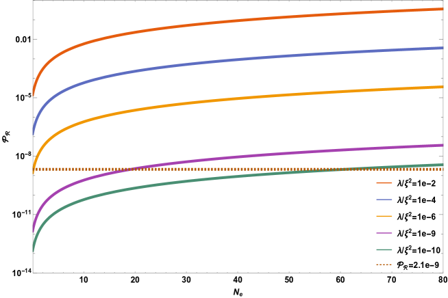
Figure 1: Scalar power spectra $\mathcal{P}_{\mathcal{R}}$ as the function of the number of e-folds $N_{e}$ with different choices of $\lambda/\xi^{2}$.

It is evident from Fig. 1 that $\mathcal{P}_{\mathcal{R}}$ attains a value of $2.1\times 10^{-9}$ at $N_{e}\sim 60$ e-folds with $\lambda/\xi^{2}=10^{-10}$.

The concept of generating PBHs is examined within a class of single-field models of inflation. In this scenario, there is a notable contrast between the dynamics on small cosmological scales and the dynamics on large scales observed through the cosmic microwave background (CMB). This disparity proves advantageous in establishing the appropriate conditions for generating PBHs. Consequently, as the perturbed scales re-enter our Universe’s horizon during later stages of radiation and subsequent matter dominance, these initial seeds undergo collapse, leading to the formation of PBHs.

The generation of substantial scalar fluctuations during the inflationary period can lead to formation of significant density fluctuations, which play a vital role in the emergence of PBHs. The study of PBHs has garnered considerable attention over years, as PHBs have the potential to contribute a significant portion or even the entirety of the dark matter content of the Universe. However, the abundance of PBHs is subject to a number of stringent constraints imposed by their gravitational effects and evaporation rate. To produce PBHs in the early Universe, the magnitude of the curvature power spectrum needs to be approximately at the order of $10^{-3}$ to $10^{-2}$. In order to satisfy a successful inflation model, the curvature power spectrum is expected to yield a value of approximately $2.1\times 10^{-9}$ at the scale of the CMB. Based on the information presented in Fig. 1, it is evident that the basic Higgs inflation model Bezrukov:2007ep lacks the ability to simultaneously address both the inflationary period and the production of PBHs. Several attempts have been made to address both scenarios, inflation and the production of PBHs, within the framework of Higgs Inflation. These attempts involve the introduction of new interactions to the Higgs field. By incorporating these additional interactions, it is possible to achieve a successful inflationary period while also generating the necessary conditions for production of PBHs Kawaguchi:2022nku ; Ezquiaga:2017fvi ; Gundhi:2020zvb ; Cheong:2019vzl ; Cheong:2022gfc .

III Modified Higgs Potential

This study examines a modified version of the Higgs potential that aims to address both the inflation and production of PBHs. Additionally, we investigate the implications of this modified potential in light of the recent NANOGrav signal NANOGrav:2023ctt . Here we are adding a Gaussian dip (bump) Mishra:2019pzq to the Higgs potential in Eq. (1). The structure of the Gaussian bump (dip) is given as follows

$$\pm\Bigg{[}Ae^{-\frac{(h(\phi)-h_{0}(\phi))^{2}}{2\sigma^{2}}}\Bigg{]}$$ (11)

After the conformal transformation, the potential transforms as

$$U_{eff}(\phi)=\frac{\lambda h^{4}(\phi)}{4}\frac{\left(1\pm Ae^{-\frac{(h(\phi)-h_{0}(\phi))^{2}}{2\sigma^{2}}}\right)}{\left(\frac{h^{2}(\phi)\xi}{M_{PL}^{2}}+1\right)^{2}}.$$ (12)

The Gaussian bump (dip) described in the above potential is featured by its height (depth) $A$ and position $h_{0}$ and width $\sigma$. The potential can be expressed in terms of the redefined field $\phi$ using equations 12 and 2. The slow roll parameters and the power spectrum for the modified Higgs potential are given in Appendix A

III.1 Parameter space search

In order to investigate the appropriate parameter space of the power spectra $\mathcal{P}_{\mathcal{R}}[A,\sigma,h_{0},\lambda,\xi]$ that yields a value of $\mathcal{P}_{\mathcal{R}}=10^{-2}-10^{-3}$ for primordial black hole (PBH) formation and $\mathcal{P}_{\mathcal{R}}=2.1\times 10^{-9}$ for a successful inflation model at the cosmic microwave background (CMB) scale, we conduct a scan over the characteristics of the bump and dip. For this analysis, we fix the Higgs self-coupling constant at $\lambda=0.1$ and the Higgs gravity coupling at $\xi=10^{4}$.

Our parameter scans reveal that the addition of a dip feature to the potential produces a desired power spectrum for PBH formation in the early stages of inflation, as depicted in Fig. 2. On the other hand, the inclusion of a bump feature in the potential only results in the required power spectrum for PBH formation at late CMB scales (see Appendix B- Fig. 6).

Figure 2 illustrates the parameter space of $\sigma$ and $N_{e}$ with varying values of $A$ and $h_{0}$. The red contour represents combinations of $\sigma$ and $N_{e}$ that yield $\mathcal{P}_{\mathcal{R}}=2.1\times 10^{-9}$ with fixed $A$ and $h_{0}$. Meanwhile, the green contour represents $\mathcal{P}_{\mathcal{R}}=1\times 10^{-2}$. We consider a range of $\sigma$ from $10^{15}$ to $10^{18}$ GeV and choose four arbitrary values for the depth of the dip $A$ (0.075, 0.1, 0.29, and 0.3). Similarly, we select four arbitrary values for the position of the dip $h_{0}$ ($1.76\times 10^{17}$ GeV, $1.8\times 10^{17}$ GeV, $2\times 10^{17}$ GeV, and $2.1\times 10^{17}$ GeV). For each combination we identify the corresponding values of $\sigma$ that yield the desired $\mathcal{P}_{\mathcal{R}}$ values for both inflation and PBH formation.

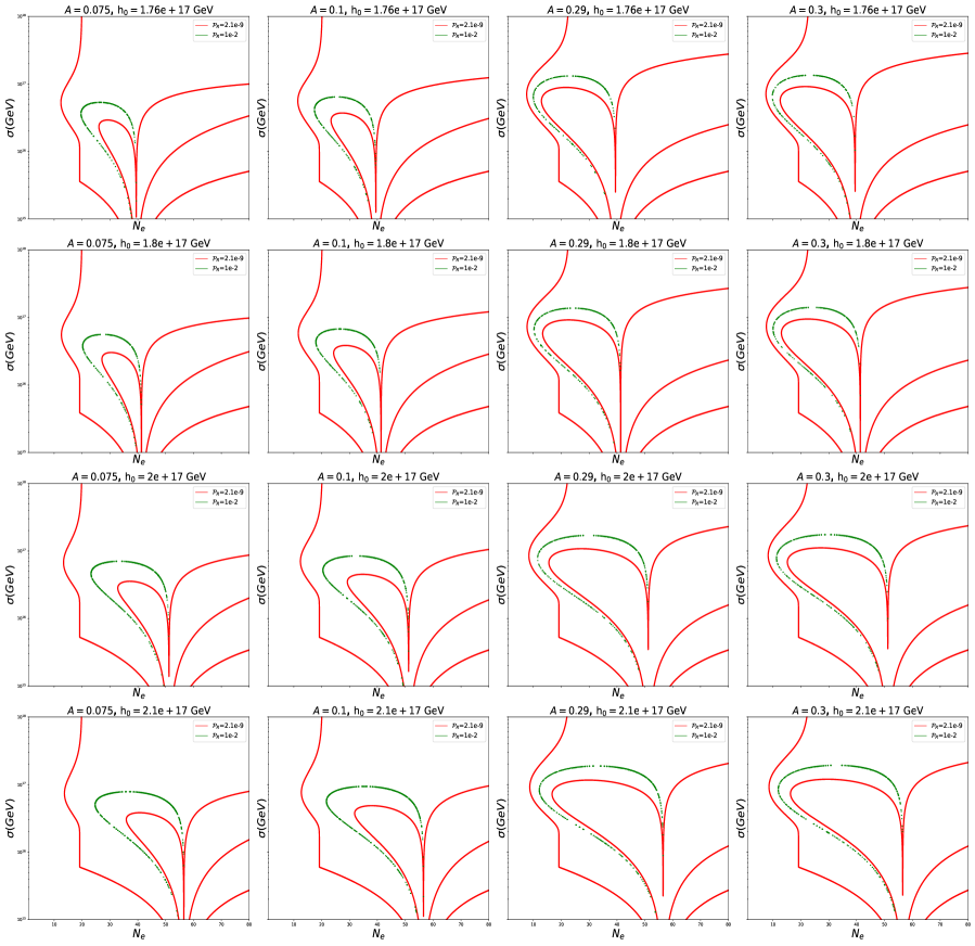
Figure 2: The contour plot illustrates the permitted parameter space of $\sigma$ and $N_{e}$ for different choices of $A$ and $h_{0}$ in the scenario of adding a dip structure, where the green contours correspond to $\mathcal{P}_{\mathcal{R}}=1\times 10^{-2}$ and the red contours correspond to $\mathcal{P}_{\mathcal{R}}=2.1\times 10^{-9}$.

By observing Fig. 3 it becomes evident that certain parameter combinations can generate the correct power spectrum for both PBH formation and inflation at CMB scales. A comparison between Fig. 3 and Fig. 1 allows us to readily identify that the inclusion of a Gaussian dip in the potential has a significant impact on the power spectrum and enabling the formation of PHB seeds.

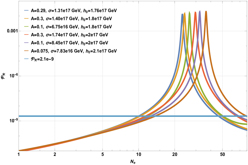
Figure 3: The power spectra $\mathcal{P}_{\mathcal{R}}$ versus the number of e-folds $N_{e}$. Here the power spectra exhibit new characteristics as a result of the addition of a Gaussian dip in the Higgs potential.

IV PBH Formation

The PBH formation requires the power spectrum to be at least $\mathcal{O}(0.01)$, the power spectrum recorded in Fig. 3 guarantees this requirement. The power spectrum has a narrow peak without oscillations. The curvature perturbation $\mathcal{R}_{k}$ is related to the density contrast by

$$\delta(t,k)=\frac{2(1+\omega)}{5+3\omega}\frac{k}{aH}\mathcal{R}_{k}\;.$$ (13)

When the perturbations reenter the horizon in the radiation-dominated era, the over-dense region in the Universe (with $\delta>\delta_{c}$) would collapse into PBHs due to the increased amplification of curvature perturbations. This collapse occurs with $\omega=1/3$ and $\delta(t,k)=\frac{4}{9}\mathcal{R}_{k}$. Since the specifics of the PBH formation process are still unclear Kehagias:2019eil ; Musco:2020jjb , the precise value of the threshold $\delta_{c}$ remains uncertain. However, if we assume a Gaussian probability distribution function for the perturbations, the mass fraction $\beta$ of PBHs at the time of their formation can be calculated.

Table 1: Inflationary observables for the different choices of the potential parameters. The resulting PBH fraction $P_{\rm PBH}$ of each region is indicated in Fig. 4. Here $N$ is the number of e-folds, $A$, $h_{0}$, and $\sigma$ are the depth, the position, and the width of the dip, respectively.

Region	A	$\rm h_{0}(GeV)$	$\rm\sigma(GeV)$	$\rm N$	$n_{s}$	$r$
a	0.29	$1.76\times 10^{17}$	$1.31\times 10^{17}$	N=47	0.950907	0.0242479
b	0.3	$1.8\times 10^{17}$	$1.40\times 10^{17}$	N=50	0.980819	0.0244824
c	0.1	$1.8\times 10^{17}$	$6.75\times 10^{16}$	N=51	0.988732	0.0300489
d	0.3	$2\times 10^{17}$	$1.74\times 10^{17}$	N=65	0.98924	0.0206994
e	0.1	$2\times 10^{17}$	$8.45\times 10^{16}$	N=68	0.98953	0.0279209
f	0.075	$2.1\times 10^{17}$	$7.83\times 10^{16}$	N=78	0.989654	0.0275894

$$\beta(M_{PBH})=2\gamma\int_{\delta_{c}}^{\infty}\frac{d\delta}{\sqrt{2\pi}\sigma_{MPH}}exp\Big{(}-\frac{\delta^{2}}{2\sigma^{2}_{PBH}}\Big{)}\simeq\sqrt{\frac{2}{\pi}}\frac{\gamma}{\nu_{c}}exp\Big{(}-\frac{\nu^{2}_{c}}{2}\Big{)}\;,$$ (14)

where $\gamma$ is the fraction of mass transformed to be PBHs that has $\delta>\delta_{c}$, and in this study, we choose $\gamma=0.4$ Gangopadhyay:2021kmf ; Garcia-Bellido:2017mdw ; Garcia-Bellido:1996mdl ; Kawaguchi:2022nku . Here $\nu_{c}=\delta_{c}/\sigma_{M_{PBH}}$ and the variance $\sigma_{M_{PBH}}$ is defined as

$$\sigma^{2}_{M_{PBH}}=\int_{0}^{\infty}\frac{dk}{k}\frac{16}{81}(kR)^{4}W^{2}(kR)\mathcal{P}_{R}(k)\;,$$ (15)

where $W(kR)$ is the window used to smooth the density contrast on comoving scale $R$. We use the Gaussian-type window function in this work,

$$W(kR)=\exp\Big{(}-\frac{k^{2}R^{2}}{2}\Big{)}.$$ (16)

The mass fraction is ultimately determined or obtained by performing the necessary calculations or calculations based on the assumptions and considerations mentioned earlierYoung:2014ana ; Gu:2022pbo .

$$\beta(M_{PBH})=\gamma\sqrt{\frac{2}{\pi}}~{}\frac{4\mathcal{P}_{R}(k)}{9\delta_{c}}exp\Big{(}-\frac{81\delta^{2}_{c}}{32\mathcal{P}_{R}(k)}\Big{)}\;.$$ (17)

The mass fraction of PBHs can be related to the abundance $f_{PBH}$ as follows when considering PBHs as a fraction of dark matter:

$$\beta(M_{PBH})=3.7\times 10^{-9}\Big{(}\frac{\gamma}{0.2}\Big{)}^{-1/2}\times\Big{(}\frac{g_{*form}}{10.75}\Big{)}^{1/4}\Big{(}\frac{M_{PBH}}{M_{\odot}}\Big{)}^{1/2}f_{PBH}\;,$$ (18)

where $M_{\odot}$ is the solar mass and $g_{*form}$ is the relativistic degrees of freedom at formation.

The mass of PBH at the formation can be written as a fraction of horizon mass given by

$$M_{PBH}=\gamma\frac{4\pi M^{2}_{P}}{H_{N}}e^{2N}$$ (19)

where $N$ is the number of e-folds during horizon exit and $H_{N}$ is the Hubble expansion rate evaluated near the inflection point. One can calculate the mass fraction of PBHs using Eq.[ 17- 19].

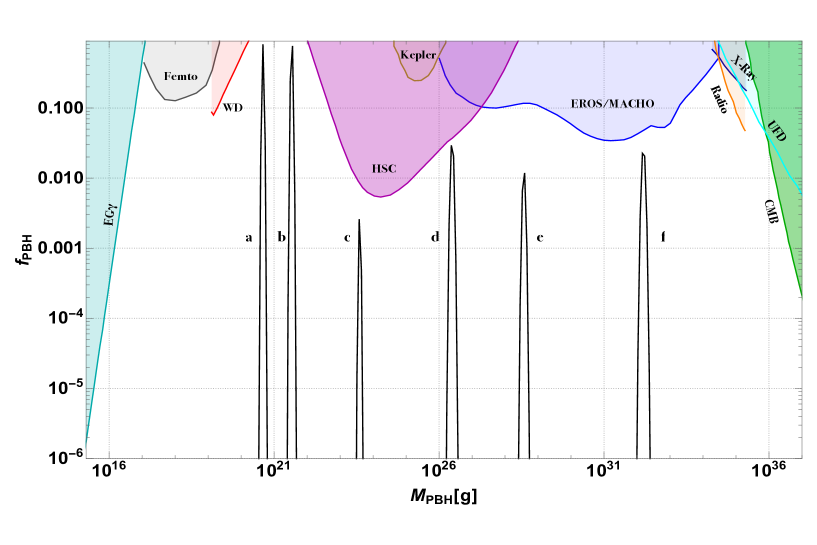
Figure 4: The fraction of PBHs as a dark matter candidate for the parameters set $\rm Region-a,b,c,d,e,$ and $f$ in Table.1. The relevant observational constraints on the current primordial black hole (PBH) mass spectrum are represented by solid lines with shades. These constraints include extra-galactic gamma-ray (EG$\gamma$) observations Carr:2009jm , femtolensing data (Femto) Barnacka:2012bm , the presence of white dwarfs in our local galaxy (WD) Graham:2015apa , Subaru HSC microlensing (HSC) results Niikura:2017zjd , Kepler milli/microlensing (Kepler) measurements Griest:2013esa , EROS/MACHO microlensing observations (EROS/MACHO) EROS-2:2006ryy , dynamical heating of ultra-faint dwarf galaxies (UFD) Brandt:2016aco , constraints from X-ray/radio observations Gaggero:2016dpq , and the accretion constraints by CMB Ali-Haimoud:2016mbv ; Aloni:2016kuh ; Horowitz:2016lib .

We obtain the abundance of PBHs as dark matter, denoted as $f_{PBH}$, for a critical threshold parameter $\delta_{c}=0.414$ Gangopadhyay:2021kmf . The corresponding results are presented in Fig. 4. Information regarding the distinct regions marked in Fig. 4 can be found in Table 1. A dip is observed with a depth of $A=0.29$ and $0.3$, accompanied by widths of $\sigma=1.31\times 10^{17}$ GeV and $1.40\times 10^{17}$ GeV, and positioned at $h_{0}=1.76\times 10^{17}$ GeV and $1.8\times 10^{17}$ GeV. This setting generates PBHs that potentially contribute to approximately $100\%$ of the dark matter, as indicated by the regions labeled $a$ and $b$ in Fig. 4.

The parameters associated with regions $a$, $b$ $c$, $d$, $e$, and $f$ produce PBHs and spectral index $n_{s}$ situated on the edge of the allowed values obtained from cosmic microwave background (CMB) observations. Moreover, these parameters have the capability to generate heavier PBHs. In our study, we conducted several parameter space scans to generate PBHs. One common feature that emerged was an increase in the depth $A$ of the potential, resulting in the production of lighter PBHs while keeping other parameters fixed. For instance, in Table 1, we observe this behavior in the case of region $b$ and $c$, where $h_{0}$ remains fixed and $A$ ranges from 0.1 to 0.3. Similarly, decreasing the value of $h_{0}$ while keeping other parameters fixed leads to a transition that yields lighter PBHs. This is exemplified by the behavior of region $d$ and $b$ in Table 1, where $A$ is fixed and $h_{0}$ varies from $2\times 10^{17}$ GeV to $1.8\times 10^{17}$ GeV.

Another noteworthy feature of the dip is that fixing both the depth $A$ and position $h_{0}$ to specific values while increasing the width $\sigma$ of the dip, would result in a reduction and eventual disappearance of the $f_{PBH}$ curve. Higher values of $\sigma$ indicate the absence of a dip, with the potential reverting to its original form and no dip effect. We have demonstrated this behavior in Appendix C, where we fixed $A=0.3$ and $h_{0}=1.8\times 10^{17}$ GeV and progressively increased the width $\sigma$.

V Stochastic second-order gravitational wave background

Production of gravitational waves through the second-order effect occurs simultaneously with the formation of PBHs, specifically when the modes re-enter the Hubble radius. Following their production, the gravitational waves propagate freely during subsequent epochs of the Universe due to their low interaction rates. The frequency of these gravitational waves corresponds to the Hubble mass at that particular time. Considering that the mass of PBHs is proportional to the Hubble mass, we can establish a relationship between the PBH mass and the present-day frequency of gravitational waves Sasaki:2018dmp .

$$f_{GW}\simeq 10^{-9}\Big{(}\frac{M_{PBH}}{30M_{\odot}}\Big{)}^{-\frac{1}{2}}~{}\text{Hz}$$ (20)

The large density perturbations not only produce the PBH dark matter but also generate the second-order gravitational wave signal Matarrese:1997ay ; Mollerach:2003nq . The current relative energy density of gravitational wave obtained from the power spectra recorded in Baumann:2007zm ; Di:2017ndc ; Halkoaho

$$\Omega_{GW}=10\mathcal{P}^{2}_{\mathcal{R}}a_{eq}$$ (21)

We choose the current scale factor $a=1$ and $a_{eq}$ is the value of scale factor at the matter radiation equality defined as

$$a_{eq}=\frac{a_{0}}{3.1\times 10^{4}~{}\Omega_{M}h^{2}},$$ (22)

where $h=\frac{H_{0}}{100km/s/Mpc}$, $H_{0}=67.27\,{\rm km}/s$ and $\Omega_{M}=0.3$. We plot $\Omega_{GW}h^{2}$ in Fig. 5.

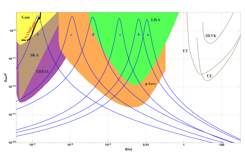
Figure 5: The gravitational wave abundance $\Omega_{\rm GW}h^{2}$ versus the frequency $f$, corresponding to the benchmark parameter sets listed in Table 1. They are compared with the recent NANOGrav 15 years sensitivity NANOGrav:2023ctt (black curve) and projecting SKA/THEIA Janssen:2014dka ; Theia:2017xtk , which utilize the observations of pulsar timing array for stochastic GW of $\mathcal{O}({\rm nHz})$. The planned GW interferometers LISA/$\mu$Ares Caprini:2015zlo ; Auclair:2019wcv ; Sesana:2019vho will cover the range from $\mu$Hz to Hz.

In the main plot (Fig. 5), our results indicate the values of $\Omega_{GW}h^{2}$, which are divided into several distinct regions. Each region is denoted and explained in Table 1.

Region f, depicted in Fig. 5, is particularly relevant as it can potentially explain the recent findings from NANOGrav NANOGrav:2023ctt . The parameter space associated with region f is characterized by a dip in the Higgs potential with a depth of $A=0.075$ and a width of $7.83\times 10^{16}$ GeV. This dip is positioned at $h_{0}=2.1\times 10^{17}$ GeV.

The relationship expressed in Eq. (20) reveals that $f_{GW}$ is proportional to $(M_{PBH})^{-1/2}$, indicating an inverse dependence between the frequency of gravitational waves ($f_{GW}$) and the mass of primordial black holes ($M_{PBH}$).

Additionally, it is worth noting that increasing the depth $A$ and shifting the position $h_{0}$ of the dip in the Higgs potential can lead to a shift in the corresponding curves towards higher frequency regimes. This observation suggests that adjustments in the parameters controlling the dip can influence the frequency spectrum of the generated gravitational waves.

VI Conclusions

In this study, we have investigated possible modifications to the classical Higgs inflation model proposed by M. Shaposhnikov and F. L. Bezrukov. We have introduced a modification to the Higgs potential by incorporating a dip at the top base of the potential. This modification has a significant impact on the generation of curvature perturbations, resulting in the amplification of second-order stochastic gravitational wave production and potential formation of PBHs. These effects were absent in the classical model.

The introduction of the dip in the potential leads to an enhancement in the power spectrum, which in turn allows for the potential existence of PBHs with masses ranging from $1.5\times 10^{20}$ g to $9.72\times 10^{32}$ g, depending on the chosen parameter space. Additionally, we have demonstrated that the selected parameter values for PBH production align with the allowed values for inflationary parameters. This suggests a consistent and viable framework for understanding the origins of PBHs and their role as potential contributors to the dark matter content of our universe.

Furthermore, we have identified specific regions within the parameter space that could account for a significant portion of the observed dark matter. By considering various cosmological constraints, we have established the consistency of these parameter regions. Additionally, we found that the resulting gravitational wave signals from our model can explain the observed excess observed by NANOGrav.

In conclusion, our study highlights the importance of the modified Higgs potential in the context of the classical Higgs inflation model. The introduced dip in the potential not only enhances the power spectrum and allows for the formation of PBHs, but also provides a promising avenue for explaining the observed excess in gravitational wave signals and addressing the dark matter puzzle in our Universe.

Appendix A Slow Roll Parameters and Power Spectrum for the Modified Higgs Potential

The slow-roll and other inflationary parameters with this effective potential (Eq. 12) can be expressed as by following Eq. (5) – Eq. (10),

$$\epsilon=\frac{\left(A\text{Mpl}^{2}\left(h\left(h^{2}-4\sigma^{2}\right)\pm h^{2}h_{0}\right)+Ah^{4}\xi\left(h\pm h_{0}\right)+4h\text{Mpl}^{2}\sigma^{2}e^{\frac{\left(h-h_{0}\right)^{2}}{2\sigma^{2}}}\right)^{2}}{12h^{6}\xi^{2}\sigma^{4}\left(A\pm e^{\frac{\left(h-h_{0}\right)^{2}}{2\sigma^{2}}}\right)^{2}}$$ (23)

Using $\epsilon$=1, we can obtain the Higgs field value at the end of inflation.

$$\eta =\frac{\pm A\left(h^{6}\xi\left(2\left(h-2h_{0}\right)\text{Mpl}^{2}+\xi\left(-2h\sigma^{2}+hh_{0}^{2}+h_{0}\sigma^{2}\right)\right)\right.}{6h^{4}h\xi^{2}\sigma^{4}\left(e^{\frac{\left(h-h_{0}\right)^{2}}{2\sigma^{2}}}\pm A\right)}$$ (24)

$$\quad+\frac{\left.h^{4}\text{Mpl}^{2}\left(\left(h-2h_{0}\right)\text{Mpl}^{2}+2\xi\left(-5h\sigma^{2}+hh_{0}^{2}+4h_{0}\sigma^{2}\right)\right)\right.}{6h^{4}h\xi^{2}\sigma^{4}\left(e^{\frac{\left(h-h_{0}\right)^{2}}{2\sigma^{2}}}\pm A\right)}$$

$$\quad+\frac{\left.h\text{Mpl}^{2}\left(h^{2}\left(h_{0}^{2}\text{Mpl}^{2}-8\sigma^{2}\left(\text{Mpl}^{2}+\xi\sigma^{2}\right)\right)+8\text{Mpl}^{2}\sigma^{4}\right)\right.}{6h^{4}h\xi^{2}\sigma^{4}\left(e^{\frac{\left(h-h_{0}\right)^{2}}{2\sigma^{2}}}\pm A\right)}$$

$$\quad+\frac{\left.7h_{0}h^{2}\text{Mpl}^{4}\sigma^{2}+\left(h-2h_{0}\right)h^{8}\xi^{2}\right)-8h\text{Mpl}^{2}\sigma^{4}e^{\frac{\left(h-h_{0}\right)^{2}}{2\sigma^{2}}}\left(h^{2}\xi-\text{Mpl}^{2}\right)}{6h^{4}h\xi^{2}\sigma^{4}\left(e^{\frac{\left(h-h_{0}\right)^{2}}{2\sigma^{2}}}\pm A\right)}$$

The number of e-folds for each case is calculated as

$$N_{e}=6\xi^{2}\int_{h_{end}}^{h_{int}}\frac{h^{3}}{\left(h^{2}\xi+\text{Mpl}^{2}\right)^{2}\left(\frac{A\left(h^{2}\pm hh_{0}\right)}{\sigma^{2}\left(e^{\frac{\left(h-h_{0}\right)^{2}}{2\sigma^{2}}}\pm A\right)}+\frac{4\text{Mpl}^{2}}{h^{2}\xi+\text{Mpl}^{2}}\right)}\,dh$$ (25)

The $\pm$ signs in equations [23]-[25] represents the bump and dip, respectively. Compared to the original model of inflation, the new modification generates complex values for $\epsilon,\eta,~{}\text{and}~{}N_{e}$. The analytical evaluation of these quantities is harder, and it is not possible to solve the Eq. (25) analytically, so we employ a numerical approach to compute the inflationary observables. The calculations of these observables, as well as the analysis of PBHs, are performed using a Python code developed by the authors. The power spectra are obtained as

$$\mathcal{P}_{\mathcal{R}}=\begin{cases}\frac{h^{8}\lambda\xi^{2}\sigma^{4}e^{-\frac{\left(h-h_{0}\right)^{2}}{2\sigma^{2}}}\left(A+e^{\frac{\left(h-h_{0}\right)^{2}}{2\sigma^{2}}}\right)^{3}}{8\pi^{2}\left(h^{2}\xi+\text{Mpl}^{2}\right)^{2}\left(A\left(hh_{0}\left(h^{2}\xi+\text{Mpl}^{2}\right)-h^{2}\text{Mpl}^{2}+h^{4}(-\xi)+4\text{Mpl}^{2}\sigma^{2}\right)+4\text{Mpl}^{2}\sigma^{2}e^{\frac{\left(h-h_{0}\right)^{2}}{2\sigma^{2}}}\right)^{2}},&\text{Potential with bump}\\ \frac{h^{8}\lambda\xi^{2}\sigma^{4}e^{-\frac{\left(h-h_{0}\right)^{2}}{2\sigma^{2}}}\left(e^{\frac{\left(h-h_{0}\right)^{2}}{2\sigma^{2}}}-A\right)^{3}}{8\pi^{2}\left(h^{2}\xi+\text{Mpl}^{2}\right)^{2}\left(A\left(-hh_{0}\left(h^{2}\xi+\text{Mpl}^{2}\right)+h^{2}\text{Mpl}^{2}+h^{4}\xi-4\text{Mpl}^{2}\sigma^{2}\right)+4\text{Mpl}^{2}\sigma^{2}e^{\frac{\left(h-h_{0}\right)^{2}}{2\sigma^{2}}}\right)^{2}},&\text{Potential with dip}\end{cases}$$ (26)

The new power spectrum is characterized by 5 parameters $[A,\sigma,h_{0},\lambda,\xi]$. By tuning these variables we can obtain the proper parameter space for the inflation, PBH production, and stochastic gravitational wave background (SGWB).

Appendix B Bump parameter space

The addition of a Gaussian bump to the Higgs Inflation model can indeed amplify the power spectra. However, such enhancements are only observed within a specific region characterized by a large number of e-folds. For PBH formation to occur, the inflationary power spectrum needs to be enhanced by a factor of $10^{7}$ within fewer than 40 e-folds of expansion.

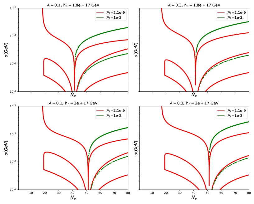
Figure 6: The contour plot illustrates the permitted parameter space of $\sigma$ and $N_{e}$ for different choices of $A$ and $h_{0}$ in the scenario of adding a bump structure, where the green contours correspond to $\mathcal{P}_{\mathcal{R}}=1\times 10^{-2}$ and the red contours correspond to $\mathcal{P}_{\mathcal{R}}=2.1\times 10^{-9}$

By comparing Figure 2 with Figure 6, it becomes evident that the current bump on the potential does not provide an adequate parameter space for PBH formation. In Fig.6 we have shown some examples of such behavior, We explore a specific parameter space characterized by a bump with a height of $A=0.1$ (or $0.3$) and positioned at $1.8\times 10^{17}$ GeV (or $2\times 10^{17}$ GeV). By scanning the values of $\sigma$ and $N_{e}$, we generate the necessary power spectra for PBH formation. It is observed that these parameter combinations are effective for generating PBHs during later and heavier epochs of inflation, as illustrated in Figure 2. Conversely, when a similar set of values is used with a dip feature in the potential, it facilitates PBH formation during smaller e-folding periods.

Appendix C PBH abundance Vs $\sigma$ values

In this section, we demonstrate, using Fig. 7, that when both the depth $A$ and position $h_{0}$ of the dip in the potential are fixed at specific values, increasing the width $\sigma$ leads to a reduction and eventual disappearance of the $f_{PBH}$ curve. Higher values of $\sigma$ indicate the absence of a dip, causing the potential to revert to its original form without a dip effect. Specifically, we set $A=0.3$ and $h_{0}=1.8\times 10^{17}$ GeV to illustrate this feature. It is important to note that this behavior can also be observed with other choices of $A$ and $h_{0}$.

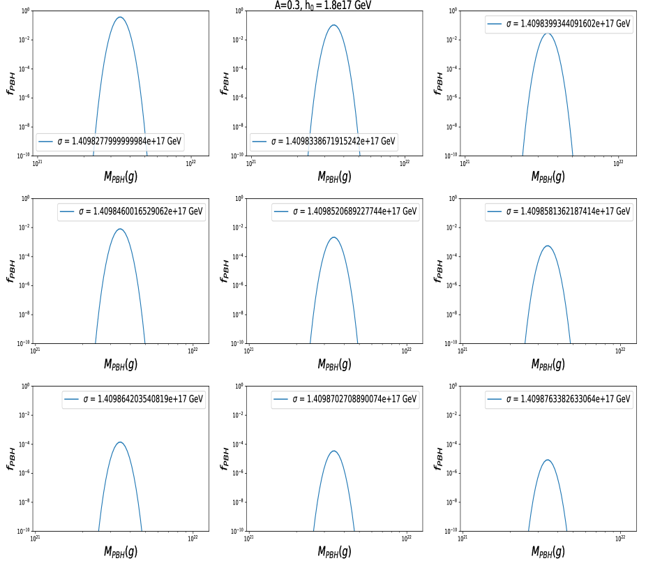
Figure 7: The corresponding PBH abundance for the benchmark parameter $A=0.3,~{}h_{0}=1.8\times 10^{17}~{}\rm GeV$ with the increment of the width $\sigma$ of the dip in the Higgs potential.

References

- (1) A. H. Guth, “The Inflationary Universe: A Possible Solution to the Horizon and Flatness Problems,” Phys. Rev. D 23 (1981), 347-356 doi:10.1103/PhysRevD.23.347
- (2) Y. B. Zel’dovich and I. D. Novikov, “The Hypothesis of Cores Retarded during Expansion and the Hot Cosmological Model,” Soviet Astron. AJ (Engl. Transl. ), 10 (1967), 602
- (3) S. Hawking, “Gravitationally collapsed objects of very low mass,” Mon. Not. Roy. Astron. Soc. 152 (1971), 75 doi:10.1093/mnras/152.1.75
- (4) B. J. Carr and S. W. Hawking, “Black holes in the early Universe,” Mon. Not. Roy. Astron. Soc. 168 (1974), 399-415 doi:10.1093/mnras/168.2.399
- (5) B. J. Carr, “The Primordial black hole mass spectrum,” Astrophys. J. 201 (1975), 1-19 doi:10.1086/153853
- (6) G. Agazie et al. [NANOGrav], “The NANOGrav 15 yr Data Set: Evidence for a Gravitational-wave Background,” Astrophys. J. Lett. 951, no.1, L8 (2023), [arXiv:2306.16213 [astro-ph.HE]].
- (7) G. Agazie et al. [NANOGrav], “The NANOGrav 15-year Data Set: Constraints on Supermassive Black Hole Binaries from the Gravitational Wave Background,” [arXiv:2306.16220 [astro-ph.HE]].
- (8) T. Broadhurst, C. Chen, T. Liu and K. F. Zheng, “Binary Supermassive Black Holes Orbiting Dark Matter Solitons: From the Dual AGN in UGC4211 to NanoHertz Gravitational Waves,” [arXiv:2306.17821 [astro-ph.HE]].
- (9) X. Niu and M. H. Rahat, “NANOGrav signal from axion inflation,” [arXiv:2307.01192 [hep-ph]].
- (10) S. Antusch, K. Hinze, S. Saad and J. Steiner, “Singling out SO(10) GUT models using recent PTA results,” [arXiv:2307.04595 [hep-ph]].
- (11) S. Vagnozzi, “Inflationary interpretation of the stochastic gravitational wave background signal detected by pulsar timing array experiments,” [arXiv:2306.16912 [astro-ph.CO]].
- (12) Z. Q. You, Z. Yi and Y. Wu, “Constraints on primordial curvature power spectrum with pulsar timing arrays,” [arXiv:2307.04419 [gr-qc]].
- (13) S. Choudhury, “Single field inflation in the light of NANOGrav 15-year Data: Quintessential interpretation of blue tilted tensor spectrum through Non-Bunch Davies initial condition,” [arXiv:2307.03249 [astro-ph.CO]].
- (14) P. Di Bari and M. H. Rahat, “The split majoron model confronts the NANOGrav signal,” [arXiv:2307.03184 [hep-ph]].
- (15) Y. Xiao, J. M. Yang and Y. Zhang, “Implications of Nano-Hertz Gravitational Waves on Electroweak Phase Transition in the Singlet Dark Matter Model,” [arXiv:2307.01072 [hep-ph]].
- (16) A. Salvio, “Supercooling in Radiative Symmetry Breaking: Theory Extensions, Gravitational Wave Detection and Primordial Black Holes,” [arXiv:2307.04694 [hep-ph]].
- (17) Y. Gouttenoire, “First-order Phase Transition interpretation of PTA signal produces solar-mass Black Holes,” [arXiv:2307.04239 [hep-ph]].
- (18) X. K. Du, M. X. Huang, F. Wang and Y. K. Zhang, “Did the nHZ Gravitational Waves Signatures Observed By NANOGrav Indicate Multiple Sector SUSY Breaking?,” [arXiv:2307.02938 [hep-ph]].
- (19) S. Wang and Z. C. Zhao, “Unveiling the Graviton Mass Bounds through Analysis of 2023 Pulsar Timing Array Datasets,” [arXiv:2307.04680 [astro-ph.HE]].
- (20) E. Babichev, D. Gorbunov, S. Ramazanov, R. Samanta and A. Vikman, “NANOGrav spectral index from melting domain walls,” [arXiv:2307.04582 [hep-ph]].
- (21) M. Geller, S. Ghosh, S. Lu and Y. Tsai, “Challenges in Interpreting the NANOGrav 15-Year Data Set as Early Universe Gravitational Waves Produced by ALP Induced Instability,” [arXiv:2307.03724 [hep-ph]].
- (22) F. L. Bezrukov and M. Shaposhnikov, “The Standard Model Higgs boson as the inflaton,” Phys. Lett. B 659 (2008), 703-706 doi:10.1016/j.physletb.2007.11.072 [arXiv:0710.3755 [hep-th]].
- (23) M. Atkins and X. Calmet, “Remarks on Higgs Inflation,” Phys. Lett. B 697 (2011), 37-40 doi:10.1016/j.physletb.2011.01.028 [arXiv:1011.4179 [hep-ph]].
- (24) J. Ren, Z. Z. Xianyu and H. J. He, “Higgs Gravitational Interaction, Weak Boson Scattering, and Higgs Inflation in Jordan and Einstein Frames,” JCAP 06 (2014), 032 doi:10.1088/1475-7516/2014/06/032 [arXiv:1404.4627 [gr-qc]].
- (25) Z. Z. Xianyu, J. Ren and H. J. He, “Gravitational Interaction of Higgs Boson and Weak Boson Scattering,” Phys. Rev. D 88 (2013), 096013 doi:10.1103/PhysRevD.88.096013 [arXiv:1305.0251 [hep-ph]].
- (26) D. Maity,“Minimal Higgs inflation,” Nucl. Phys. B 919 (2017), 560-568 doi:10.1016/j.nuclphysb.2017.04.005 [arXiv:1606.08179 [hep-ph]].
- (27) J. Rubio, “Higgs inflation,” Front. Astron. Space Sci. 5 (2019), 50 doi:10.3389/fspas.2018.00050 [arXiv:1807.02376 [hep-ph]].
- (28) M. He, A. A. Starobinsky and J. Yokoyama, “Inflation in the mixed Higgs- model,” JCAP 05 (2018), 064 doi:10.1088/1475-7516/2018/05/064 [arXiv:1804.00409 [astro-ph.CO]].
- (29) K. Kamada, T. Kobayashi, T. Takahashi, M. Yamaguchi and J. Yokoyama, “Generalized Higgs inflation,” Phys. Rev. D 86 (2012), 023504 doi:10.1103/PhysRevD.86.023504 [arXiv:1203.4059 [hep-ph]].
- (30) C. J. Ouseph and K. Cheung, “Higgs Inflation with four-form couplings,” J. Phys. G 48 (2021) no.5, 055001 doi:10.1088/1361-6471/abefa4 [arXiv:2002.12010 [hep-ph]].
- (31) O. Lebedev and H. M. Lee, “Higgs Portal Inflation,” Eur. Phys. J. C 71 (2011), 1821 doi:10.1140/epjc/s10052-011-1821-0 [arXiv:1105.2284 [hep-ph]].
- (32) C. Germani and A. Kehagias, “New Model of Inflation with Non-minimal Derivative Coupling of Standard Model Higgs Boson to Gravity,” Phys. Rev. Lett. 105 (2010), 011302 doi:10.1103/PhysRevLett.105.011302 [arXiv:1003.2635 [hep-ph]].
- (33) D. S. Salopek, J. R. Bond and J. M. Bardeen, “Designing Density Fluctuation Spectra in Inflation,” Phys. Rev. D 40 (1989), 1753 doi:10.1103/PhysRevD.40.1753
- (34) D. I. Kaiser, “Primordial spectral indices from generalized Einstein theories,” Phys. Rev. D 52 (1995), 4295-4306 doi:10.1103/PhysRevD.52.4295 [arXiv:astro-ph/9408044 [astro-ph]].
- (35) E. Komatsu and T. Futamase, “Complete constraints on a nonminimally coupled chaotic inflationary scenario from the cosmic microwave background,” Phys. Rev. D 59 (1999), 064029 doi:10.1103/PhysRevD.59.064029 [arXiv:astro-ph/9901127 [astro-ph]].
- (36) D. I. Kaiser, “Conformal Transformations with Multiple Scalar Fields,” Phys. Rev. D 81 (2010), 084044 doi:10.1103/PhysRevD.81.084044 [arXiv:1003.1159 [gr-qc]].
- (37) R. M. Wald, “General Relativity,” doi:10.7208/chicago/9780226870373.001.0001
- (38) D. H. Lyth and A. Riotto, “Particle physics models of inflation and the cosmological density perturbation,” Phys. Rept. 314 (1999), 1-146 doi:10.1016/S0370-1573(98)00128-8 [arXiv:hep-ph/9807278 [hep-ph]].
- (39) P. A. R. Ade et al. [Planck], “Planck 2015 results. XX. Constraints on inflation,” Astron. Astrophys. 594 (2016), A20 doi:10.1051/0004-6361/201525898 [arXiv:1502.02114 [astro-ph.CO]].
- (40) P. A. R. Ade et al. [BICEP2 and Keck Array], “BICEP2 / Keck Array x: Constraints on Primordial Gravitational Waves using Planck, WMAP, and New BICEP2/Keck Observations through the 2015 Season,” Phys. Rev. Lett. 121 (2018), 221301 doi:10.1103/PhysRevLett.121.221301 [arXiv:1810.05216 [astro-ph.CO]].
- (41) R. Kawaguchi and S. Tsujikawa, “Primordial black holes from Higgs inflation with a Gauss-Bonnet coupling,” Phys. Rev. D 107 (2023) no.6, 063508 doi:10.1103/PhysRevD.107.063508 [arXiv:2211.13364 [astro-ph.CO]].
- (42) J. M. Ezquiaga, J. Garcia-Bellido and E. Ruiz Morales, “Primordial Black Hole production in Critical Higgs Inflation,” Phys. Lett. B 776 (2018), 345-349 doi:10.1016/j.physletb.2017.11.039 [arXiv:1705.04861 [astro-ph.CO]].
- (43) A. Gundhi and C. F. Steinwachs, “Scalaron–Higgs inflation reloaded: Higgs-dependent scalaron mass and primordial black hole dark matter,” Eur. Phys. J. C 81 (2021) no.5, 460 doi:10.1140/epjc/s10052-021-09225-2 [arXiv:2011.09485 [hep-th]].
- (44) D. Y. Cheong, S. M. Lee and S. C. Park, “Primordial black holes in Higgs- inflation as the whole of dark matter,” JCAP 01 (2021), 032 doi:10.1088/1475-7516/2021/01/032 [arXiv:1912.12032 [hep-ph]].
- (45) D. Y. Cheong, K. Kohri and S. C. Park, “The inflaton that could: primordial black holes and second order gravitational waves from tachyonic instability induced in Higgs-R 2 inflation,” JCAP 10 (2022), 015 doi:10.1088/1475-7516/2022/10/015 [arXiv:2205.14813 [hep-ph]].
- (46) G. Agazie et al. [NANOGrav], “The NANOGrav 15 yr Data Set: Detector Characterization and Noise Budget,” Astrophys. J. Lett. 951 (2023) no.1, L10 doi:10.3847/2041-8213/acda88 [arXiv:2306.16218 [astro-ph.HE]].
- (47) S. S. Mishra and V. Sahni, “Primordial Black Holes from a tiny bump/dip in the Inflaton potential,” JCAP 04 (2020), 007 doi:10.1088/1475-7516/2020/04/007 [arXiv:1911.00057 [gr-qc]].
- (48) A. Kehagias, I. Musco and A. Riotto, “Non-Gaussian Formation of Primordial Black Holes: Effects on the Threshold,” JCAP 12 (2019), 029 doi:10.1088/1475-7516/2019/12/029 [arXiv:1906.07135 [astro-ph.CO]].
- (49) I. Musco, V. De Luca, G. Franciolini and A. Riotto, “Threshold for primordial black holes. II. A simple analytic prescription,” Phys. Rev. D 103 (2021) no.6, 063538 doi:10.1103/PhysRevD.103.063538 [arXiv:2011.03014 [astro-ph.CO]].
- (50) M. R. Gangopadhyay, J. C. Jain, D. Sharma and Yogesh, “Production of primordial black holes via single field inflation and observational constraints,” Eur. Phys. J. C 82 (2022) no.9, 849 doi:10.1140/epjc/s10052-022-10796-x [arXiv:2108.13839 [astro-ph.CO]].
- (51) J. Garcia-Bellido and E. Ruiz Morales, “Primordial black holes from single field models of inflation,” Phys. Dark Univ. 18 (2017), 47-54 doi:10.1016/j.dark.2017.09.007 [arXiv:1702.03901 [astro-ph.CO]].
- (52) J. Garcia-Bellido, A. D. Linde and D. Wands, “Density perturbations and black hole formation in hybrid inflation,” Phys. Rev. D 54 (1996), 6040-6058 doi:10.1103/PhysRevD.54.6040 [arXiv:astro-ph/9605094 [astro-ph]].
- (53) S. Young, C. T. Byrnes and M. Sasaki, “Calculating the mass fraction of primordial black holes,” JCAP 07 (2014), 045 doi:10.1088/1475-7516/2014/07/045 [arXiv:1405.7023 [gr-qc]].
- (54) B. M. Gu, F. W. Shu, K. Yang and Y. P. Zhang, “Primordial black holes from an inflationary potential valley,” Phys. Rev. D 107 (2023) no.2, 023519 doi:10.1103/PhysRevD.107.023519 [arXiv:2207.09968 [astro-ph.CO]].
- (55) B. J. Carr, K. Kohri, Y. Sendouda and J. Yokoyama, “New cosmological constraints on primordial black holes,” Phys. Rev. D 81 (2010), 104019 doi:10.1103/PhysRevD.81.104019 [arXiv:0912.5297 [astro-ph.CO]].
- (56) A. Barnacka, J. F. Glicenstein and R. Moderski, “New constraints on primordial black holes abundance from femtolensing of gamma-ray bursts,” Phys. Rev. D 86 (2012), 043001 doi:10.1103/PhysRevD.86.043001 [arXiv:1204.2056 [astro-ph.CO]].
- (57) P. W. Graham, S. Rajendran and J. Varela, “Dark Matter Triggers of Supernovae,” Phys. Rev. D 92 (2015) no.6, 063007 doi:10.1103/PhysRevD.92.063007 [arXiv:1505.04444 [hep-ph]].
- (58) H. Niikura, M. Takada, N. Yasuda, R. H. Lupton, T. Sumi, S. More, T. Kurita, S. Sugiyama, A. More and M. Oguri, et al. “Microlensing constraints on primordial black holes with Subaru/HSC Andromeda observations,” Nature Astron. 3 (2019) no.6, 524-534 doi:10.1038/s41550-019-0723-1 [arXiv:1701.02151 [astro-ph.CO]].
- (59) K. Griest, A. M. Cieplak and M. J. Lehner, “New Limits on Primordial Black Hole Dark Matter from an Analysis of Kepler Source Microlensing Data,” Phys. Rev. Lett. 111 (2013) no.18, 181302 doi:10.1103/PhysRevLett.111.181302
- (60) P. Tisserand et al. [EROS-2], “Limits on the Macho Content of the Galactic Halo from the EROS-2 Survey of the Magellanic Clouds,” Astron. Astrophys. 469 (2007), 387-404 doi:10.1051/0004-6361:20066017 [arXiv:astro-ph/0607207 [astro-ph]].
- (61) T. D. Brandt, “Constraints on MACHO Dark Matter from Compact Stellar Systems in Ultra-Faint Dwarf Galaxies,” Astrophys. J. Lett. 824 (2016) no.2, L31 doi:10.3847/2041-8205/824/2/L31 [arXiv:1605.03665 [astro-ph.GA]].
- (62) D. Gaggero, G. Bertone, F. Calore, R. M. T. Connors, M. Lovell, S. Markoff and E. Storm, “Searching for Primordial Black Holes in the radio and X-ray sky,” Phys. Rev. Lett. 118 (2017) no.24, 241101 doi:10.1103/PhysRevLett.118.241101 [arXiv:1612.00457 [astro-ph.HE]].
- (63) Y. Ali-Haïmoud and M. Kamionkowski, “Cosmic microwave background limits on accreting primordial black holes,” Phys. Rev. D 95 (2017) no.4, 043534 doi:10.1103/PhysRevD.95.043534 [arXiv:1612.05644 [astro-ph.CO]].
- (64) D. Aloni, K. Blum and R. Flauger, JCAP 05 (2017), 017 doi:10.1088/1475-7516/2017/05/017 [arXiv:1612.06811 [astro-ph.CO]].
- (65) B. Horowitz, “Revisiting Primordial Black Holes Constraints from Ionization History,” [arXiv:1612.07264 [astro-ph.CO]].
- (66) M. Sasaki, T. Suyama, T. Tanaka and S. Yokoyama, “Primordial black holes—perspectives in gravitational wave astronomy,” Class. Quant. Grav. 35 (2018) no.6, 063001 doi:10.1088/1361-6382/aaa7b4 [arXiv:1801.05235 [astro-ph.CO]].
- (67) S. Matarrese, S. Mollerach and M. Bruni, “Second order perturbations of the Einstein-de Sitter universe,” Phys. Rev. D 58 (1998), 043504 doi:10.1103/PhysRevD.58.043504 [arXiv:astro-ph/9707278 [astro-ph]].
- (68) S. Mollerach, D. Harari and S. Matarrese, “CMB polarization from secondary vector and tensor modes,” Phys. Rev. D 69 (2004), 063002 doi:10.1103/PhysRevD.69.063002 [arXiv:astro-ph/0310711 [astro-ph]].
- (69) D. Baumann, P. J. Steinhardt, K. Takahashi and K. Ichiki, “Gravitational Wave Spectrum Induced by Primordial Scalar Perturbations,” Phys. Rev. D 76 (2007), 084019 doi:10.1103/PhysRevD.76.084019 [arXiv:hep-th/0703290 [hep-th]].
- (70) H. Di and Y. Gong, “Primordial black holes and second order gravitational waves from ultra-slow-roll inflation,” JCAP 07 (2018), 007 doi:10.1088/1475-7516/2018/07/007 [arXiv:1707.09578 [astro-ph.CO]].
- (71) Johannes Halkoaho and Syksy Räsänen, “Primordial black holes and gravitational waves from inflation-Master Thesis,”
- (72) G. Janssen, G. Hobbs, M. McLaughlin, C. Bassa, A. T. Deller, M. Kramer, K. Lee, C. Mingarelli, P. Rosado and S. Sanidas, et al. “Gravitational wave astronomy with the SKA,” PoS AASKA14, 037 (2015), [arXiv:1501.00127 [astro-ph.IM]].
- (73) C. Boehm et al. [Theia], “Theia: Faint objects in motion or the new astrometry frontier,” [arXiv:1707.01348 [astro-ph.IM]].
- (74) C. Caprini, M. Hindmarsh, S. Huber, T. Konstandin, J. Kozaczuk, G. Nardini, J. M. No, A. Petiteau, P. Schwaller and G. Servant, et al. “Science with the space-based interferometer eLISA. II: Gravitational waves from cosmological phase transitions,” JCAP 04, 001 (2016),[arXiv:1512.06239 [astro-ph.CO]].
- (75) P. Auclair, J. J. Blanco-Pillado, D. G. Figueroa, A. C. Jenkins, M. Lewicki, M. Sakellariadou, S. Sanidas, L. Sousa, D. A. Steer and J. M. Wachter, et al. “Probing the gravitational wave background from cosmic strings with LISA,” JCAP 04, 034 (2020),[arXiv:1909.00819 [astro-ph.CO]].
- (76) A. Sesana, N. Korsakova, M. A. Sedda, V. Baibhav, E. Barausse, S. Barke, E. Berti, M. Bonetti, P. R. Capelo and C. Caprini, et al. “Unveiling the gravitational universe at -Hz frequencies,” Exper. Astron. 51, no.3, 1333-1383 (2021),[arXiv:1908.11391 [astro-ph.IM]].