Finite element inspired networks: Learning interpretable
deformable object dynamics from partial observations

Abstract

Accurate simulation of deformable linear object (DLO) dynamics is challenging if the task at hand requires a human-interpretable model that also yields fast predictions. To arrive at such a model, we draw inspiration from the rigid finite element method (R-FEM) and model a DLO as a serial chain of rigid bodies whose internal state is unrolled through time by a dynamics network. As this state is not observed directly, the dynamics network is trained jointly with a physics-informed encoder which maps observed motion variables to the DLO’s hidden state. To encourage that the state acquires a physically meaningful representation, we leverage the forward kinematics of the underlying R-FEM model as a decoder. Through robot experiments we demonstrate that the proposed architecture provides an easy-to-handle, yet capable DLO dynamics model yielding physically interpretable predictions from partial observations. The project code is available at: https://tinyurl.com/fei-networks

I Introduction

Deformable linear objects (DLOs), such as cables, ropes, and threads, are prevalent in various promising applications within the field of robotics [1, 2]. Dynamics models empower robots to interact with DLOs, showcasing remarkable dexterity at tasks such as intricate knotting [3, 4], precise manipulation of ropes [5], and surgical suturing [6, 7]. Furthermore, there are many robots which contain parts that can be modeled as DLOs. This naturally applies to numerous soft robots but is also relevant for the control of supposedly rigid industrial robots. For example, the significant end-effector forces arising in robot machining cause elastic deformations which, if not modeled accurately, reduce manufacturing precision [8, 9]. In addition, designing lightweight yet flexible manipulators and legged robots potentially lowers the robot’s manufacturing costs, increases its maximum attainable joint accelerations, and benefits its energy efficiency [10].

Learning robot dynamics is challenging as the amount of real data (as opposed to simulation data) is limited, and the data’s coverage of the robot’s state space depends on the control strategy employed for data collection. Therefore, purely data-driven models, such as neural networks (NNs), often fall short of expectations when it comes to learning DLO dynamics [1, 2]. Furthermore, these models lack interpretability. A promising approach to enhancing both the sample efficiency and interpretability of data-driven DLO dynamics models is to incorporate first-principled knowledge from physics into the model’s architecture. Physics-inspired models often enforce a physically plausible state representation in the network’s architecture, such as the Lagrangian [11, 12], which subsequently improves the model’s sample efficiency and interpretability. Typically, such models are tested on rigid robots whose states are directly observed.

In contrast to rigid robots, a DLO is a continuous accumulation of mass, making it unclear what the state representation should be and how to estimate it in the first place. Fortunately, we can draw inspiration from the literature on the R-FEM and the articulated body algorithm to pursue the simple yet compelling idea:

Model DLO dynamics as a chain of rigid bodies whose interactions are learned from data.

This approach combines the strengths of R-FEM and machine learning. On one hand, it provides a physically interpretable model where states pertain to generalized coordinates of rigid bodies, in contrast to black-box models whose states do not have physical meaning [13]. On the other hand, analytically modeling interactions between those bodies becomes difficult, particularly for coarse R-FEM discretizations with few rigid bodies. By learning these interactions, we obtain a computationally fast and accurate model suitable, e.g. for model-based control of DLOs.

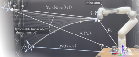
Figure 1: A DLO (Aluminium rod) is actuated by a robot arm. Given an initial observation of $\{\mathrm{e}\}$’s translational state $y_{k}$ and $\{\mathrm{b}\}$’s position, velocity and state-acceleration vector from $t_{k}$ to $t_{k+N}$, $x_{k:k+N-1}$, a FEI network predicts $y_{k+1:k+N}$ while also estimating the DLO’s shape encoded in the hidden state $h=[q_{\text{rfem}},\dot{q}_{\text{rfem}}]$.

Building upon the aforementioned idea, at a high level, our work addresses the following problem: given measurements of positions, velocities and accelerations of one end of a deformable object, predict the position and velocity of the other end over time. Ultimately, we aim to use such a model for solving DLO manipulation tasks, thus we additionally prioritize models that are computationally fast and can be used within model predictive controllers. The proposed method is validated on an experimental setup as shown in Fig. 1, which provides an overview of the setup and the main notation used. The notation $\{B\}$ refers to an inertial coordinate frame, while $\{\text{b}\}$ and $\{\text{e}\}$ denote frames fixed to the DLO’s start and end, respectively. Throughout the subsequent sections, the networks hidden state is $h=[q_{\text{rfem}},\dot{q}_{\text{rfem}}]\in\mathbb{R}^{n_{h}}$. A dataset $\mathcal{D}$ contains trajectories consisting of the position and linear velocity of $\{\text{e}\}$ with respect to $\{B\}$, denoted by $y=[p_{\text{e}},\dot{p}_{\text{e}}]\in\mathbb{R}^{n_{y}}$ and the position, velocity, and acceleration of $\{\text{b}\}$ with respect to $\{B\}$, denoted as $x=[q_{\text{b}},\dot{q}_{\text{b}},\ddot{q}_{\text{b}}]\in\mathbb{R}^{n_{x}}$. Following this notation, we define the problem addressed in this work as follows:

Given an initial observation $y_{k}$ and a sequence of future inputs $x_{k:k+N-1}:=[x_{k},\dots,x_{k+N-1}]$, predict future observations $y_{k+1:k+N}:=[y_{k+1},\dots,y_{k+N}]$.

To address this problem, we propose the finite element inspired (FEI) network, which consists of four essential components: 1) a physics-informed encoder that maps $y_{k}$ and $x_{k}$ to a hidden state $h_{k}$, 2) a dynamics network that predicts $h_{k+1}$ from $h_{k}$ and $x_{k}$, 3) a decoder that maps $h_{k}$ and $x_{k}$ to $y_{k}$, and 4) a loss function that regularizes $h$ during training. Summarizing, the contributions of this work are:

1. We propose a novel FEI network that learns to predict the motion of a DLO from partial observations.

2. We demonstrate that leveraging the forward kinematics of a DLO’s R-FEM discretization as a decoder effectively enforces a human-interpretable network state.

3. Through robot experiments on two DLOs with different material properties, we demonstrate that FEI networks offer physically interpretable predictions with accuracy on par with purely data-driven black-box models.

II Related Work

The literature on DLO dynamics models can be classified based on the knowledge utilized for model synthesis, which includes employing first principles from physics or system-specific data. While we structure the related work along these lines, the main contribution of our work revolves around describing and observing the DLO’s hidden state using forward kinematics arising from an R-FEM discretization. Therefore, special emphasis is placed on the type of observations that are used by the different DLO dynamics models.

Analytical physics-based models

Numerous works explore physics-based dynamics modeling of DLOs [14, 10, 15]. For an in-depth discussion of the mechanics underlying DLO, the interested reader is referred to [16] and the references therein. The dynamics of DLOs can be conceptualized as an aggregation of infinitesimally small mass particles that interact through forces. To render the complicated particle interactions tractable for computational analysis, the finite element method aggregates the continuous distribution of particles into finite elements. The R-FEM assumes that all particles inside an element form a rigid body such that their distances to each other remain fixed [17]. The R-FEM’s approximation results in a simplified representation of the DLO’s dynamics, but its accuracy relies on the chosen force function determining element interactions and its parameters. While many analytical models for these components exist, they often do not suffice when using small element counts or modeling DLOs with heterogeneous material properties. As R-FEM lies at the heart of our work, we discuss it in more detail in Section III.

Other commonly found DLO dynamics models use finite differences approximations [18, 16] or piecewise constant curvature models [19], which arise from a simplification of the Cosserat rod model [20, 6]. Stella et al. employed curvatures to model the dynamics of a 2D underwater tentacle [21] and the kinematics of a 3D soft-continuum robot [22].

	System	Dynamics model	State type	Observed
[21]	Submerged tentacle (2D)	constant curvature	Splines	Full state
[23]	Submerged tentacle (2D)	echo state network	Points	Full state
[24]	DLO in magnetic field	LSTMs	Points	Full state
[5]	Rope moved by robot arm	bi-LSTM	Mass particles	Full state
[25]	DLO attached to robot arm	bi-LSTM + Graph NN	Mass particles	Full state
[13]	DLO attached to robot arm	LSTM	Black box	DLO ends
Ours	DLO attached to robot arm	flexible (e.g., RNN, ResNet)	Rigid bodies	DLO ends

TABLE I: Overview of related literature on data-driven modeling of DLO dynamics. While numerous works focus on the dynamics identification and observe the DLO’s full state through cameras, [13] and our work learns the dynamics by solely observing frames attached to the DLO’s start and end. Moreover, while previous literature focuses on a particular model architecture to learn dynamics, we focus on leveraging kinematics such that some dynamics model learns a physical meaningful representation.

Data-driven models

Table I presents a summary of related data-driven DLO dynamics models. Our research is inspired by [13], who employed a long short-term memory (LSTM) network [26] to capture the input-output dynamics of a robot-arm-held foam cylinder. In this study, the authors utilize the LSTM to predict the DLO’s endpoint positions from the pitch and yaw angles of the DLO’s beginning held by the robot arm. The LSTM’s hidden state lacks a physically meaningful representation hindering the formulation of constraints on the DLO’s shape, particularly during manipulation in an environment with obstacles. FEI network alleviates this limitation.

In related works, [23, 24] employed camera-based techniques to estimate the DLO’s center-line as a sequence of points. In [24], the dynamics of each point are predicted by an LSTM that shares with the other LSTMs its output history. Similarly, [23] introduced echo state networks, where the output of an RNN serves as the input for a second RNN, in addition to control inputs and bending sensor measurements. In [5], the authors developed a quasi-static model of a DLO using a bi-directional LSTM (bi-LSTM) whose state is estimated from camera images using a convolutional neural network. Unlike previous works that used LSTMs to propagate states in time, the bi-LSTM propagates information along both directions of the DLO’s spatial dimension. Inspired by [5], [25] combined bi-LSTMs with graph neural networks [27]. In particular, [25] discretizes the DLO into a sequence of cylindrical elements similar to Cosserat theory [6] while the spatial and temporal element interactions are modeled through the NNs. However, these seminal works require cameras to obtain an estimation of several points on the DLO and operate at low velocities where quasi-static models are sufficient for predicting states. The proposed FEI network allows to extend these methods to operate on partial observations and in dynamic scenarios.

Numerous other works explore learning dynamics purely in simulation. As these work do not encounter the many challenges of real-world robotics, they can focus solely on the algorithmic-side of combining physics with machine learning. In this domain, one often encounters the “Encoder-Processor-Decoder” network structure that we also adopt in the FEI network. For example, [28] uses this structure to learn the dynamics of particle systems via GNNs. In [28], all particle positons are observed and the model predicts acceleration which is then numerically integrated. In comparison, the FEI network uses the encoder as a state observer while its processor (aka “dynamics network”) simulates the DLO’s hidden discrete-time dynamics. In turn, one could further extend the FEI network by replacing its dynamics network with a GNN as proposed in [28].

III Rigid FEM for modeling DLOs

As R-FEM lies at the core of the FEI network, in what follows, we give a brief introduction to R-FEM for modeling a DLO as a chain of $n_{\text{el}}+1$ rigid bodies.

III-A Kinematics

As illustrated in Fig. 2, the pose of the $i$-th body in the chain is described via a body-fixed coordinate frame $\{i\}$. The pose of $\{\mathrm{e}\}$ with respect to $\{\mathrm{B}\}$ is described by the homogeneous transformation matrix

$${}^{\mathrm{B}}T_{\mathrm{e}}=\begin{bmatrix}{}^{\mathrm{B}}R_{\mathrm{e}}&{}^{\mathrm{B}}p_{\mathrm{e},\mathrm{B}}\\ 0&1\end{bmatrix}\in\text{SE}(3)$$ (1)

with the position vector ${}^{\mathrm{B}}p_{\mathrm{e},\mathrm{B}}\in\mathbb{R}^{3}$, rotation matrix ${}^{\mathrm{B}}R_{\mathrm{e}}$, and $\text{SE}(3)$ denoting the special Euclidean group [29]. Note that we omit the superscripts and subscripts if a vector or matrix is either expressed in the inertia frame $\{B\}$ or it points from $\{B\}$’s origin such that $p_{\mathrm{e}}:={}^{\mathrm{B}}p_{\mathrm{e},\mathrm{B}}$ and $R_{\text{e}}:={}^{\mathrm{B}}R_{\mathrm{e}}$. In a chain of $n_{\text{el}}+1$ bodies ${}^{\text{b}}p_{\text{e},\text{b}}$ is obtained as

$$\begin{bmatrix}{}^{\mathrm{b}}p_{\mathrm{e},\mathrm{b}}\\ 1\end{bmatrix}={}^{\mathrm{b}}T_{1}(q_{1})\cdot{}^{1}T_{2}(q_{2})\cdot...\cdot{}^{n_{\text{el}}-1}T_{n_{\text{el}}}(q_{n_{\text{el}}})\begin{bmatrix}{}^{n_{\text{el}}}p_{\mathrm{e},n_{\text{el}}}\\ 1\end{bmatrix},$$

where $q_{\text{rfem}}=[q_{1},...,q_{n_{\text{el}}}]$ denotes the generalized coordinates of the DLO’s rigid body chain approximation and ${}^{i-1}T_{i}(q_{i})$ transforms a (homogeneous) vector from $\{i\}$ to $\{i-1\}$ [29, p. 93]. In addition, $q_{\mathrm{b}}=[p_{\mathrm{b}},\Psi_{\mathrm{b}}]$ defines the six degrees of freedoms (DOF) of the floating-base $\{\mathrm{b}\}$. For modeling the relative motion of bodies in the serial chain, we use 2D revolute joints as depicted in Fig. 2. While translatory DOFs are described through translation vectors $p$, various parametrizations $\Psi$ exist that describe rotational DOFs. Typically used rotation descriptions are Euler angles, quaternions, exponential coordinates [29], and position-twist angle pairs [30]. The DLO’s endpoint position is obtained as

$$p_{\mathrm{e}}=\mathrm{fk}(q_{\mathrm{b}},q_{\text{rfem}})\coloneqq R_{\text{b}}(\Psi_{\mathrm{b}})\,{}^{\mathrm{b}}p_{\text{e},\text{b}}(q_{\text{rfem}})+p_{\mathrm{b}}$$ (2)

As detailed in [31, p. 111], differential kinematics describes the relation between $\dot{q}_{\text{b}}$, $\dot{q}_{\text{rfem}}$, and $\dot{p}_{\text{e}}$ via the joint Jacobian matrix $J_{\text{lin}}(q_{\text{b}},q_{\text{rfem}})$ as

$$\dot{p}_{\text{e}}=J_{\text{lin}}(q_{\text{b}},q_{\text{rfem}})\begin{bmatrix}\dot{q}_{\text{b}}\\ \dot{q}_{\text{rfem}}\end{bmatrix}=\begin{bmatrix}\frac{\partial\text{fk}}{\partial q_{\text{b}}}&\frac{\partial\text{fk}}{\partial q_{\text{rfem}}}\end{bmatrix}\begin{bmatrix}\dot{q}_{\text{b}}\\ \dot{q}_{\text{rfem}}\end{bmatrix}.$$ (3)

Equation (2) and (3) form the forward kinematics function that maps elements in $h_{k}$ and $x_{k}$ to $y_{k}$.

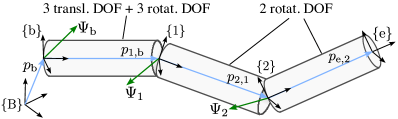
Figure 2: Generalized coordinate representations of a body chain with $n_{\text{el}}=2$. The chain’s joint states are described through rotation parameters $\Psi_{i}$ that provide two rotational DOF to each element.

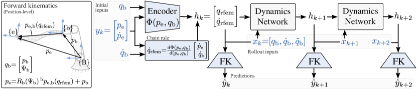
Figure 3: Architecture of an FEI network with rollout length $N=2$. By resorting to forward kinematics (FK) of a body chain and taking inspiration from R-FEM to determine the inputs, the model learns a physically-plausible hidden state from partial observations.

III-B Dynamics

Designing an FEI network requires making informed decisions regarding the quantities that should be observed and fed into the model. We can draw inspiration from multibody dynamics to understand the causal structure needed for propagating the state of the DLO over time. For a rigid body chain, the Newton-Euler equations establish the relationship between the forces and torques acting on bodies and inside joints to the bodies’ accelerations $\ddot{q}=[\ddot{q}_{\text{b}},\ddot{q}_{\text{rfem}}]\in\mathbb{R}^{n_{q}}$ resulting in the equation of motion

$$M(q)\ddot{q}=c(q,\dot{q})+\tau(q,\dot{q})$$ (4)

with the generalized inertia matrix $M(\cdot)\in\mathbb{R}^{n_{q}\times n_{q}}$, the bias force $c(q,\dot{q})\in\mathbb{R}^{n_{q}}$ and the joint torques $\tau(q,\dot{q})$ [32, 29]. The formulation of the dynamics depends on what quantities are being observed and which quantities we aim to predict. This gives rise to different types of dynamics formulations, namely forward dynamics, inverse dynamics, or hybrid dynamics. In the case of forward dynamics, the joint torques are known inputs, and the model outputs joint acceleration. Conversely, inverse dynamics involves predicting the joint torques based on the given joint acceleration.

When dealing with a DLO manipulated by a robot arm, the dynamics are governed by hybrid dynamics. That is, for the first body attached to $\{\mathrm{b}\}$, the acceleration $\ddot{q}_{b}$ is provided, while the corresponding joint torque $\tau_{b}$ remains unobserved. For the subsequent bodies in the chain, our objective is to predict the accelerations $\ddot{q}_{\text{rfem}}$ as a function of the joint torques $\tau_{\text{rfem}}(q_{\text{rfem}},\dot{q}_{\text{rfem}})$. An efficient implementation of hybrid dynamics is detailed in [33]. This algorithm provides valuable insight into the input-output structure of the hybrid dynamics of a rigid body chain. In particular, the hybrid dynamics algorithm given in [33] is a function of the form

$$\ddot{q}_{\text{rfem}}=f_{\text{HybDyn}}(h,x,\theta_{\text{P}}),$$ (5)

where $\theta_{\text{P}}$ is a vector of constant mechanical parameters (e.g., element length, mass, and inertia). A prediction of the next state is obtained by rewriting (5) in continuous state-space form $\dot{h}=f(h,x,\theta_{\text{P}})$ and numerically integrating, reading

$$h_{k+1}=\mathrm{ODESolve}(f,h_{k},x_{k},\Delta t),$$ (6)

where $\Delta t=t_{k+1}-t_{k}$ is the integration step size and $\mathrm{ODESolve}(\cdot)$ refers to a numerical integration method.

IV Finite Element Inspired Networks

FEI network consists of three essential components as shown in the Fig. 3: a physics-informed encoder that maps initial observation $y_{k}$ and input $x_{k}$ into a hidden state $h_{k}$; a dynamics network that propagates states using inputs $x_{k},\dots,x_{k+N}$; and an analytical decoder – forward kinematics (FK) of the R-FEM approximation of a DLO – that maps hidden states and inputs into observations $y_{k},\dots,y_{k+N}$. Recall that R-FEM approximates a DLO by a serial chain of rigid bodies connected via elastic joints. By deploying the FK of this chain as a decoder, we enforce that the network latent state represents the state of such a chain. This approach not only grants physical interpretability to the model but also enables the learning of DLO dynamics from partial observations, facilitates the reconstruction of the DLO’s shape, and paves the way for new avenues in physics-informed machine learning of DLO dynamics.

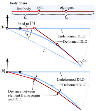
Figure 4: Errors arising in a rigid body chain approximation of a DLO with $n_{\text{el}}=2$ and fixed element length. Top: If the chain’s first body is fixed to $\{b\}$ then errors arise in the prediction of the DLO’s end position $p_{\text{e}}$. Bottom: If the first body can rotate freely and the element length is fixed, then the distances between the element frame origins and the DLO may increase.

IV-A Approximation errors of finite element inspired networks

Initially when setting up the FEI network, we adopted a uniform discretization method [17] as commonly used in R-FEM. This discretization assumes constant element lengths $L_{\mathrm{el}}$ while the first and last body in the chain are set to $L_{\mathrm{el}}/2$. Naturally, for small element counts, such a discretization spawns significant approximation errors.

As illustrated in Fig. 4 (Top), fixing the first body to $\{\text{b}\}$ causes an error $\epsilon_{\mathrm{el}}$ in the FEI network’s prediction of the DLO end’s position $p_{\text{e}}$. An upper bound for $\epsilon_{\mathrm{el}}$ is obtained using the law of cosines, writing

$$\epsilon_{\mathrm{el}}<\sqrt{L^{2}+L_{1}^{2}-2LL_{1}\cos(\zeta)}-L_{2}$$ (7)

with the DLO’s length $L=L_{1}+L_{2}$, the length of the first body $L_{1}=L_{\mathrm{el}}/2$, the length of all the other elements $L_{2}=(n_{\text{el}}-0.5)L_{\mathrm{el}}$, and the deflection angle $\zeta$ as depicted in Fig. 4 (Top). In turn, the discretization error $\epsilon_{\mathrm{el}}$ due to fixing the first body to $\{\mathrm{b}\}$ is upper bounded by (7) if the deformed DLO’s end point $p_{\text{e}}$ remains in a cone with angle $\zeta$ and slant height $L$. Fig. 5 plots the upper bound on $\epsilon_{\mathrm{el}}$ for different $\zeta$ and $n_{\text{el}}$. The approximation error can be decreased by reducing $L_{1}$. While we initially discretize the DLO as shown in Fig. 4 (Top), we reduce $\epsilon_{\mathrm{el}}$ by learning the length of the bodies alongside the FEI network’s other parameters as detailed in Section IV-E.

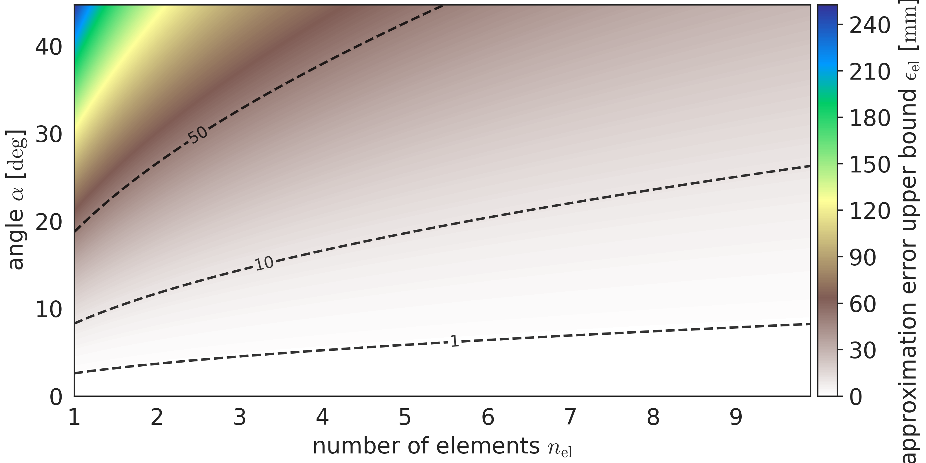
Figure 5: Upper bound on the error $\epsilon_{\mathrm{el}}$ caused by fixing the first body to $\{b\}$ and setting its length to $L_{\mathrm{el}}/2$ plotted over different element numbers $n_{\text{el}}$ and deflection angles $\zeta$. The DLO’s length amounts to $L=1920\,\mathrm{mm}$.

IV-B Decoder

The decoder in the FEI network is inspired by the kinematics description of a serial chain of rigid bodies. The decoder equals the FK as given by (2) and (3). By using such a decoder, we ensure the interpretability of a NN that models the DLO’s dynamics, while maintaining a physically meaningful relationship between the hidden states.

To derive an FK decoder, we specify the type of joint (e.g., XY Euler angles), provide the DLO’s overall length, select the number of elements $n_{\text{el}}$, and use [17] to obtain the initial element lengths. To address the afore mentioned limitations of an uniform discretization, we learn element lengths being denoted as $\theta_{\text{el}}=[l_{1},\dots,l_{n_{\text{el}}+1}]$. To prevent the length from becoming arbitrarily large, we penalize the deviation of the estimated total length from the DLO’s actual length.

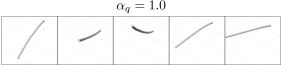
Figure 6: Aluminium rod DLO shape predicted by a FEI network with $n_{\text{el}}=7$.

IV-C Encoder

The encoder, predicts $q_{\text{rfem}}=\Phi(p_{\text{e}},q_{\text{b}})$ which corresponds to learning the inverse kinematics of a serial chain. Internally, the encoder performs two key transformations before feeding the data into a feed-forward NN. The transformations include: i) computing the vector $p_{\mathrm{e},\mathrm{b}}=p_{\mathrm{e}}-p_{\mathrm{b}}$ to leverage that $q_{\text{rfem}}$ is independent to translations of the DLO in space and improve the encoder’s generalization performance; ii) computing $\sin(\cdot)$ and $\cos(\cdot)$ of the Euler angles $\Phi_{b}$ to avoid discontinuities in the angle parametrization. The velocities $\dot{q}_{\text{rfem}}$ are obtained by differentiating the encoder as

$$\dot{q}_{\text{rfem}}=\frac{\partial\Phi}{\partial p_{\text{e}}}\dot{p}_{\text{e}}+\frac{\partial\Phi}{\partial q_{\text{b}}}\dot{q}_{\text{b}},$$ (8)

which is straightforward to implement with automatic differentiation libraries such as JAX [34]. Note that (8) ensures that the velocity $\dot{q}_{\text{rfem}}$ is the time derivative of $q_{\text{rfem}}$ which is not the case if we let a NN predict $\dot{q}_{\text{rfem}}$. If $\text{dim}(q_{\text{rfem}})>\text{dim}([p_{\text{e}},q_{\text{b}}])$, learning inverse kinematics from observations becomes an ill-posed problem [35]. After all, multiple chain configurations $q_{\text{rfem}}$ achieve the same end frame pose.

IV-D Dynamics Network

The dynamics network is responsible for unrolling the hidden state $h$ over time, serving a similar role as the analytical hybrid dynamics presented in equations (5) and (6). Assuming that R-FEM is suitable for modeling a DLO, these equations indicate that the only input needed for unrolling $h$ in time is $x=[q_{\text{b}},\dot{q}_{\text{b}},\ddot{q}_{\text{b}}]$. While in our experiments we attain precise estimates of $\ddot{q}_{\text{b}}$, future versions of FEI networks could draw inspiration from [28] and replace $\ddot{q}_{\text{b}}$ with past velocity observations. If one would observe the robot’s end-effector force $\tau_{\text{b}}$, then the dynamics network could learn forward dynamics by replacing $x$ with the input $x^{\prime}=[q_{\text{b}},\dot{q}_{\text{b}},\tau_{\text{b}}]$.

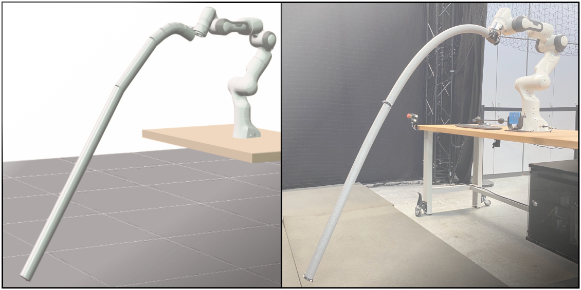
Figure 7: Left: Shape of a foam cylinder predicted by an FEI network with $n_{\text{el}}=7$ and the element length being learned alongside other parameters. Right: Foam cylinder DLO actuated by a robot arm.

DLO	$L$, m	$\rho,\ \text{kg/m}^{3}$	$E$, Pa	$\eta,\ \text{Ns/m}$
Aluminum rod	1.92	2710	$5.15\cdot 10^{10}$	$1.2\cdot 10^{8}$
Foam cylinder	1.90	105	$1.8\cdot 10^{6}$	$3.5\cdot 10^{5}$

TABLE II: Physical parameters of the first principal models with the Young’s modulus $E$ and normal damping coefficient $\eta$.

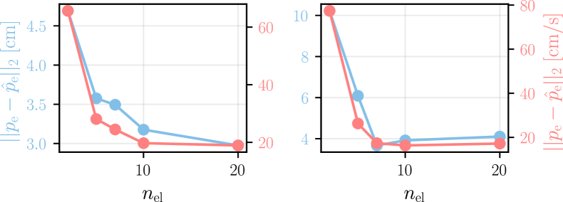
Figure 8: Influence of the element count $n_{\text{el}}$ on the FEI network’s prediction error of $p_{\mathrm{e}}$ (blue color) and $\dot{p}_{\text{e}}$ (red color). Left: Aluminium rod. Right: Foam cylinder.

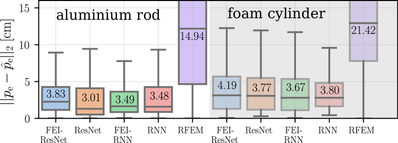
Figure 9: RMSE of FEI- and black-box models on test data trajectories with rollout length $N=250$ (1 s prediction horizon). The numbers inside the boxes denote mean values.

IV-E Loss Regularization

While we hypothesized that joint training of forward kinematics and dynamics may regularize $q_{\text{rfem}}$, we observed that without loss regularization, the encoder does not acquire a physically plausible state representation in its efforts to assist the dynamics network. Therefore, we introduce a regularization term in the FEI network’s loss, writing

$$\mathcal{L}_{\mathrm{FEI}}=\frac{1}{n_{b}N}\sum_{j=1}^{n_{b}}\sum_{k=1}^{N}w_{k}||y_{k,j}-\hat{y}_{k,j}||_{W_{y}}^{2}+\mathcal{L}_{\mathrm{reg}}(q_{\text{rfem}},\dot{q}_{\text{rfem}}),$$ (9)

with the regularization loss

$$\mathcal{L}_{\mathrm{reg}}=\underbrace{\alpha_{q}\|q_{\text{rfem},k,j}\|_{2}^{2}}_{\mathcal{L}_{P}}+\underbrace{\alpha_{\dot{q}}\|\dot{q}_{\text{rfem},k,j}\|_{2}^{2}}_{\mathcal{L}_{K}}+\mathcal{L}_{\text{FK}}(\theta_{\text{el}},\theta_{\text{eb}})$$ (10)

and further the batch size $n_{b}$, the model’s predictions $\hat{y}_{k,j}$, the weighting matrix $W_{y}\in\mathbb{R}^{6\times 6}$, the state weight $w_{k}$, regularization parameters $\alpha_{q}$ and $\alpha_{\dot{q}}$, and additional kinematics regularization losses $\mathcal{L}_{\text{FK}}$. While the latter two terms in (10) can be simply seen as $\ell_{2}$ regularization of the hidden state $h$, we can look at these terms through the lens of R-FEM. In this regard, $\mathcal{L}_{P}$ in (10) represents a potential energy of linear spring forces acting between the elements while $\mathcal{L}_{K}$ represents the chain’s kinetic energy. While the kinetic energy of the rigid body chain depends on the inertia matrix $M(q_{\text{rfem}})$, it is lower and upper bounded by positive real constants $\kappa_{1}\leq M(q_{\text{rfem}})\leq\kappa_{2}$ [31]; thus, justifies the choice of $\mathcal{L}_{K}$. We can reconstruct the DLO’s shape from the FEI network’s hidden state $h$. As illustrated in Fig. 6, the chain’s shape depends on the choice of $\alpha_{q}$. Finally, $\mathcal{L}_{\text{FK}}$ reads

$$\mathcal{L}_{\text{FK}}=\alpha_{L}\left(\sum\theta_{\text{el}}-L\right)+\alpha_{\text{el}}\|\theta_{\text{el}}-\theta_{\text{el}}^{\prime}\|_{2}^{2}+\alpha_{\text{eb}}\|\theta_{\text{eb}}-\theta_{\text{eb}}^{\prime}\|_{2}^{2},$$ (11)

with $\theta_{\text{el}}^{\prime}$ denoting the initial element lengths obtained as in [17], $\theta_{\text{eb}}$ denoting the calibration error arising in the observation of ${}^{\mathrm{b}}p_{\mathrm{e},\mathrm{b}}$, and $\theta_{\text{eb}}^{\prime}$ denoting the same error estimate obtained from prior calibration routines. The first two terms in (11) enable the FEI network to reduce $\epsilon_{\mathrm{el}}$ by estimating the element lengths $\theta_{\text{el}}$ as shown in Fig. 7. To account for calibration errors in the observation of ${}^{\mathrm{b}}p_{\mathrm{e},\mathrm{b}}$, we introduce $\theta_{\text{eb}}$ to the kinematics encoder model and also optimize its entries during training. The third term in (11) ensures that $\theta_{\text{eb}}$ remains close to $\theta_{\text{eb}}^{\prime}$.

V Results

To analyze the performance of different FEI networks, we learn to predict the motion of two physical DLOs with different properties that are rigidly connected to a Franka Panda robot arm. The two DLO’s are: i) an aluminum rod as depicted in Fig. 1 (1.92 m length, 4 mm inner diameter, 6 mm outer diameter), ii) a polyethylene foam cylinder as depicted in Fig. 7 (1.90 m length, 60 mm outer diameter).

V-A Experimental Setup

To measure the DLO motion, two marker frames are attached to each DLO’s start and end. A ”Vicon” camera-based positiong system records the motion of these frames.

Calibration

The raw sensor readings are obtained in different frames. To accurately express measurements in the same frames, we calibrated the following constant transformations: the transformation from the Panda base frame $\{\text{B}\}$ to the table frame $\{\text{t}\}$; the transformation from the flange frame $\{\text{f}\}$ to the DLO start frame $\{\mathrm{b}\}$; and the distance between the origins of frames $\{\mathrm{b}\}$ and $\{\mathrm{e}\}$ in the DLO’s resting position.

Trajectory design

To excite the dynamics of the DLO, we employed the multisine trajectory

$$\dot{q}_{\text{p}}(t)=A\cos(Wt)-B\sin(Wt)$$ (12)

as a reference for the Panda joint velocity controller where $A$ and $B$ represent multisine coefficients, $W$ corresponds to the harmonics. $A$ and $B$ are obtained from the solution of a constrained optimization problem such that the end-effector acceleration is maximized while adhering to the physical limits of the Panda robot. The selection of harmonics $W$ determines which eigenfrequencies of the DLO’s dynamics are being excited.

	Position RMSE $[\mathrm{cm}]$
	$N$	$2N$	$5N$	$10N$	$20N$
R-FEM	14.9	16.9	20.0	21.2	22.5
ResNet	3.0	11.3	45.2	62.3	73.0
FEI-ResNet (ours)	3.8	4.6	6.7	7.0	7.3
RNN	3.5	4.2	5.9	7.0	7.1
FEI-RNN (ours)	3.5	4.2	6.6	7.1	7.9
	Velocity RMSE $[\mathrm{cm/s}]$
	$N$	$2N$	$5N$	$10N$	$20N$
R-FEM	91	95.1	114.4	120.1	126.3
ResNet	22.0	150.0	607.1	860.0	979.7
FEI-ResNet (ours)	24.7	29.6	47.6	49.3	51.8
RNN	23.0	27.7	38.7	45.5	46.4
FEI-RNN (ours)	24.5	29.8	48.1	51.7	57.6

TABLE III: RMSE of $p_{\text{e}}$ and $\dot{p}_{\text{e}}$ with training rollout length $N{=}250$ for differing prediction rollout lengths.

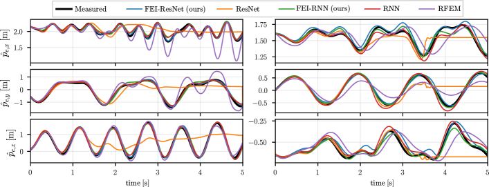
Figure 10: Model rollouts with a prediction horizon being five times longer than during training. Left: Aluminum rod. Right: Foam cylinder.

Data Collection

During data collection, we recorded the Panda’s joint positions $q_{\text{p}}$ and velocities $\dot{q}_{\text{p}}$, as well as marker frame poses with the Vicon system. During the data processing stage, we computed the observations $y$ and inputs $x$ using the calibrated kinematics and forward kinematics of the robot arm. The Vicon system and the robot operate at different maximum sampling frequencies (Vicon system: $\sim 300$ Hz, Robot arm: $\sim 600$ Hz). To ensure that data is collected at the same frequency and eliminate high-frequency noise, we processed the raw data using the following steps: 1) Expressed the Vicon measurements in the robot base frame $\{\text{B}\}$. 2) Constructed a uniform grid with a sampling time of $\Delta t=0.004$ ms 3) Designed zero-phase low-pass Butterworth filter of order 8, sampling frequency $1/\Delta t$ and cut-off frequency $f_{\mathrm{co}}=3.5$ Hz. The filter’s cut-off frequency was chosen using the joint-torque reference signal as ground truth. 4) For Panda data: (i) resampled $q_{\text{p}}$ and $\dot{q}_{\text{p}}$ to a uniform grid and applied the designed filter; (ii) computed $\ddot{q}_{\text{p}}$ using central differences. For Vicon data: (i) resampled $p_{\text{e}}$ to a uniform grid and applied the designed filter; (ii) computed $\dot{p}_{\text{e}}$ using central differences. 5) Computed pose $(p_{\text{b}},\ \Psi_{\text{b}})$ and its two derivative using the robot arm’s FK.

We collected twelve different trajectories for the aluminum rod and eight trajectories for the foam cylinder. During the first half of each trajectory (about 15 seconds) the robot arm moved the DLO; during the second half, the robot arm rested while the DLO kept moving. For the aluminum rod, nine trajectories were used for training and validation, while for the foam cylinder seven trajectories were collected. The trajectories were divided into rollouts of length $N=250$ using a rolling window approach, corresponding to one second of motion. Then, rollouts were split into training and validation data sets with ratio 85 % and 15 %, respectively. The remaining trajectories of the DLO’s were used for testing and divided into rollouts using a sliding window method.

V-B Model Settings

As the FEI’s dynamics network, we used RNN with Gated Recurrent Units [36] and ResNets [37] – and denote the resulting models as FEI-RNN and FEI-ResNet, respectively. As data-driven baselines, we combine the same models with fully connected MLPs acting as encoder and decoder denoting the resulting models as RNN and ResNet. Note that the MLP encoder predicts the full state $h$ without enforcing $\dot{q}_{\text{rfem}}=dq_{\text{rfem}}/dt$. As a first-principle baseline, we employ R-FEM with the manually tuned parameters provided in Table II. The FEI models are trained using the loss function (9) while the baseline NNs use an $\ell_{2}$ loss. All models were implemented in JAX [34] using the Equinox library [38]. Further details are provided in the attached code repository.

V-C Experimental Results

Element Count

Fig. 8 depicts the RMSE of the FEI-RNN model’s predictions on the test data. Initially, increasing the number of elements substantially reduces the error. This observation aligns with the common knowledge that discretization-based methods, like R-FEM, show improved model accuracy for increasing element counts. However, beyond seven elements, the marginal improvement in prediction accuracy does not justify the increased computational cost associated with model evaluation, which is crucial for enabling efficient model-based control. Therefore, for the remainder of this paper, we adopt $n_{\text{el}}=7$.

Prediction Accuracy & Computation Time

Fig. 9 shows the prediction accuracy of the considered models evaluated on test trajectories of the same length ($N=250$ corresponding to a prediction horizon of 1 second) as the training rollouts. Data-driven models significantly outperform the first-principle model (RFEM). The models more accurately predict the aluminum rod’s motion than the foam cylinder, possibly due to variations in training data or material properties.

All the models yield stable predictions during rollouts that extend significantly beyond $N$, as depicted in Fig. 10. However, the ResNet exhibits a noticeable drop in prediction accuracy as the prediction length exceeds $N$. In contrast, the FEI-ResNet does not show this issue. Table III shows the model’s RMSE of the prediction of $p_{\text{e}}$ and $\dot{p}_{\text{e}}$ for the aluminium rod. Our findings indicate that models incorporating NN encoders and decoders slightly outperform the FEI models in terms of prediction accuracy. We posit that the decoder imposes constraints on the model which slightly reduces the model’s expressiveness. Among models with a NN decoder, the RNN has a smaller RMSE than the ResNet for all rollouts except for the one of length $N$. In comparison, the FEI networks’ RMSE at $20N$ is slightly worse than RMSEs of the RNN.

In terms of training time, FEI models are slower to train due to the nonlinear forward kinematics and the physics-informed encoder, which requires gradient computations during forward passes, as illustrated in Fig. 3. Since the trained models may be used for model-based control, we analysed the models computation times. The FEI-RNN model has a computation time of $\sim\,1$ ms for a rollout of length $N$ and the FEI-ResNet model of about $5$ ms.

Physical interpretability

FEI networks possess a a physically meaningful state representation compared to black-box models such as RNN and ResNet. In this regard, FEI networks hidden state represents elastic joints positions and velocities of serial chain of rigid bodies that approximate the DLO. Therefore, it is possible to approximately reconstruct the shape of the DLO through forward kinematics from a partial observation $y$ and an input $x$, as shown in the Fig. 7. This property is especially valuable in manipulation tasks involving obstacles.

VI Conclusion

We have presented the first data-driven DLO dynamics model capable of accurately learning the motion of a DLO from partial observations while also acquiring a human interpretable hidden state representation. Our model successfully predicted the position and velocity of a 1.92 m long aluminum rod and a 1.90 m long polyethylene foam cylinder. Despite the endpoints of the DLO deviating up to 1.5 m from their equilibrium position, the trained FEI model achieved a sub-decimeter RMSE in a twenty-second simulation. This model was obtained by first deriving the forward kinematics of a rigid body chain approximating the DLO. At the first step of a rollout, the DLO’s hidden state is reconstructed from partial observations of the DLO’s start and end frames using an MLP encoder. In the subsequent time steps, the hidden state is unrolled through time using a NN that effectively learns the system’s dynamics. All networks are trained jointly while we regularize the hidden state to ensure that it acquires a physically plausible hidden state representation.

References

- [1] J. Sanchez, J.-A. Corrales, B.-C. Bouzgarrou, and Y. Mezouar, “Robotic manipulation and sensing of deformable objects in domestic and industrial applications: a survey,” The International Journal of Robotics Research, vol. 37, no. 7, pp. 688–716, 2018.
- [2] P. Jiménez, “Survey on model-based manipulation planning of deformable objects,” Robotics and computer-integrated manufacturing, vol. 28, no. 2, pp. 154–163, 2012.
- [3] W. Wang, D. Berenson, and D. Balkcom, “An online method for tight-tolerance insertion tasks for string and rope,” in 2015 IEEE International Conference on Robotics and Automation (ICRA). IEEE, 2015, pp. 2488–2495.
- [4] E. Yoshida, K. Ayusawa, I. G. Ramirez-Alpizar, K. Harada, C. Duriez, and A. Kheddar, “Simulation-based optimal motion planning for deformable object,” in 2015 IEEE international workshop on advanced robotics and its social impacts (ARSO). IEEE, 2015, pp. 1–6.
- [5] M. Yan, Y. Zhu, N. Jin, and J. Bohg, “Self-supervised learning of state estimation for manipulating deformable linear objects,” IEEE Robotics and Automation Letters, vol. 5, no. 2, pp. 2372–2379, 2020.
- [6] D. K. Pai, “Strands: Interactive simulation of thin solids using cosserat models,” in Computer graphics forum, vol. 21. Wiley Online Library, 2002, pp. 347–352.
- [7] M. Saha and P. Isto, “Manipulation planning for deformable linear objects,” IEEE Transactions on Robotics, vol. 23, no. 6, 2007.
- [8] A. Karim and A. Verl, “Challenges and obstacles in robot-machining,” in IEEE ISR 2013, 2013, pp. 1–4.
- [9] A. Verl, A. Valente, S. Melkote, C. Brecher, E. Ozturk, and L. T. Tunc, “Robots in machining,” CIRP Annals, vol. 68, no. 2, pp. 799–822, 2019.
- [10] S. Drücker and R. Seifried, “Application of stable inversion to flexible manipulators modeled by the absolute nodal coordinate formulation,” GAMM-Mitteilungen, vol. 46, no. 1, 2023.
- [11] M. Lutter, C. Ritter, and J. Peters, “Deep lagrangian networks: Using physics as model prior for deep learning,” in International Conference on Learning Representations, 2019.
- [12] M. Cranmer, S. Greydanus, S. Hoyer, P. Battaglia, D. Spergel, and S. Ho, “Lagrangian neural networks,” in ICLR 2020 Workshop on Integration of Deep Neural Models and Differential Equations, 2019.
- [13] J. A. Preiss, D. Millard, T. Yao, and G. S. Sukhatme, “Tracking fast trajectories with a deformable object using a learned model,” in 2022 International Conference on Robotics and Automation (ICRA), 2022, pp. 1351–1357.
- [14] J. Spillmann and M. Teschner, “Corde: Cosserat rod elements for the dynamic simulation of one-dimensional elastic objects,” in Proceedings of the 2007 ACM SIGGRAPH/Eurographics symposium on Computer animation, 2007, pp. 63–72.
- [15] J. Kim and N. S. Pollard, “Fast simulation of skeleton-driven deformable body characters,” ACM Transactions on Graphics (TOG), vol. 30, no. 5, pp. 1–19, 2011.
- [16] M. Bergou, M. Wardetzky, S. Robinson, B. Audoly, and E. Grinspun, “Discrete elastic rods,” in ACM SIGGRAPH 2008, 2008, pp. 1–12.
- [17] E. Wittbrodt, I. Adamiec-Wójcik, and S. Wojciech, Dynamics of flexible multibody systems: rigid finite element method. Springer Science & Business Media, 2007.
- [18] H. Lang, J. Linn, and M. Arnold, “Multi-body dynamics simulation of geometrically exact cosserat rods,” Multibody System Dynamics, vol. 25, no. 3, pp. 285–312, 2011.
- [19] R. J. Webster III and B. A. Jones, “Design and kinematic modeling of constant curvature continuum robots: A review,” The International Journal of Robotics Research, vol. 29, no. 13, pp. 1661–1683, 2010.
- [20] J. Till, V. Aloi, and C. Rucker, “Real-time dynamics of soft and continuum robots based on cosserat rod models,” The International Journal of Robotics Research, vol. 38, no. 6, pp. 723–746, 2019.
- [21] F. Stella, N. Obayashi, C. D. Santina, and J. Hughes, “An experimental validation of the polynomial curvature model: Identification and optimal control of a soft underwater tentacle,” IEEE Robotics and Automation Letters, vol. 7, no. 4, pp. 11 410–11 417, 2022.
- [22] F. Stella, Q. Guan, C. Della Santina, and J. Hughes, “Piecewise affine curvature model: a reduced-order model for soft robot-environment interaction beyond pcc,” in 2023 IEEE International Conference on Soft Robotics (RoboSoft), 2023, pp. 1–7.
- [23] K. Tanaka, Y. Minami, Y. Tokudome, K. Inoue, Y. Kuniyoshi, and K. Nakajima, “Continuum-body-pose estimation from partial sensor information using recurrent neural networks,” IEEE Robotics and Automation Letters, vol. 7, no. 4, pp. 11 244–11 251, 2022.
- [24] A. Tariverdi, V. K. Venkiteswaran, M. Richter, O. J. Elle, J. Tørresen, K. Mathiassen, S. Misra, and Ø. G. Martinsen, “A recurrent neural-network-based real-time dynamic model for soft continuum manipulators,” Frontiers in Robotics and AI, vol. 8, p. 631303, 2021.
- [25] Y. Yang, J. A. Stork, and T. Stoyanov, “Learning to propagate interaction effects for modeling deformable linear objects dynamics,” in 2021 IEEE International Conference on Robotics and Automation (ICRA). IEEE, 2021, pp. 1950–1957.
- [26] S. Hochreiter and J. Schmidhuber, “Long short-term memory,” Neural computation, vol. 9, no. 8, pp. 1735–1780, 1997.
- [27] F. Scarselli, M. Gori, A. C. Tsoi, M. Hagenbuchner, and G. Monfardini, “The graph neural network model,” IEEE transactions on neural networks, vol. 20, no. 1, pp. 61–80, 2008.
- [28] A. Sanchez-Gonzalez, J. Godwin, T. Pfaff, R. Ying, J. Leskovec, and P. Battaglia, “Learning to simulate complex physics with graph networks,” in International conference on machine learning. PMLR, 2020, pp. 8459–8468.
- [29] K. M. Lynch and F. C. Park, Modern robotics. Cambridge University Press, 2017.
- [30] B. Lefevre, F. Tayeb, L. Du Peloux, and J.-F. Caron, “A 4-degree-of-freedom kirchhoff beam model for the modeling of bending–torsion couplings in active-bending structures,” International Journal of Space Structures, vol. 32, no. 2, pp. 69–83, 2017.
- [31] B. Siciliano, L. Sciavicco, L. Villani, and G. Oriolo, “Modelling, planning and control,” Advanced Textbooks in Control and Signal Processing. Springer,, 2009.
- [32] R. Featherstone, “Rigid body dynamics algorithms,” 2014.
- [33] J. Kim, “Lie group formulation of articulated rigid body dynamics,” Technical report, Carnegie Mellon University, Tech. Rep., 2012.
- [34] J. Bradbury, R. Frostig, P. Hawkins, M. J. Johnson, C. Leary, D. Maclaurin, G. Necula, A. Paszke, J. VanderPlas, S. Wanderman-Milne, and Q. Zhang, “JAX: composable transformations of Python+NumPy programs,” 2018. [Online]. Available: http://github.com/google/jax
- [35] M. I. Jordan, “Constrained supervised learning,” Journal of Mathematical Psychology, vol. 36, no. 3, pp. 396–425, 1992.
- [36] K. Cho, B. Van Merriënboer, C. Gulcehre, D. Bahdanau, F. Bougares, H. Schwenk, and Y. Bengio, “Learning phrase representations using rnn encoder-decoder for statistical machine translation,” arXiv preprint arXiv:1406.1078, 2014.
- [37] K. He, X. Zhang, S. Ren, and J. Sun, “Deep residual learning for image recognition,” in Proceedings of the IEEE conference on computer vision and pattern recognition, 2016, pp. 770–778.
- [38] P. Kidger and C. Garcia, “Equinox: neural networks in JAX via callable PyTrees and filtered transformations,” Differentiable Programming workshop at Neural Information Processing Systems 2021, 2021.