Heteroscedastic Causal Structure Learning

Abstract

Heretofore, learning the directed acyclic graphs (DAGs) that encode the cause-effect relationships embedded in observational data is a computationally challenging problem. A recent trend of studies has shown that it is possible to recover the DAGs with polynomial time complexity under the equal variances assumption. However, this prohibits the heteroscedasticity of the noise, which allows for more flexible modeling capabilities, but at the same time is substantially more challenging to handle. In this study, we tackle the heteroscedastic causal structure learning problem under Gaussian noises. By exploiting the normality of the causal mechanisms, we can recover a valid causal ordering, which can uniquely identifies the causal DAG using a series of conditional independence tests. The result is HOST (Heteroscedastic causal STructure learning), a simple yet effective causal structure learning algorithm that scales polynomially in both sample size and dimensionality. In addition, via extensive empirical evaluations on a wide range of both controlled and real datasets, we show that the proposed HOST method is competitive with state-of-the-art approaches in both the causal order learning and structure learning problems.

1 Introduction

Causal structure learning provides the crucial knowledge to answer not only the statistically descriptive questions of the systems of interest, but also interventional and counterfactual queries. Thus, it is at the heart of interest in many sciences where cause-effect relationships are of utmost concerns, such as bioinformatics [26], econometric [12], and neural sciences [3]. However, this problem poses serious challenges when no prior knowledge is available, not to mention the limitation of its practical solvability with respect to the scale of data.

Constraint-based [30, 31, 6] and score-based methods [5, 21, 20, 38, 39] are conventionally two main approaches in causal structure learning. The former branch leverages a series of statistical tests to eliminate implausible connections between the variables of interest, but the number of tests can grow exponentially with the number of variables. Meanwhile, the latter group assigns dedicated scores to each candidate causal graph based on data fitness, then performs greedy search or continuous optimization for the optimal answer with respect to the defined score, which is a NP-Hard problem since the space of possible DAGs is super-exponentially large in the number of variables [24]. Both of these approaches cannot eliminate all improbable solutions without further experimentations or prior knowledge, so the result is a class of causal graphs that can induce the same observed data, also known as the Markov Equivalent Class (MEC).

Recently, there is a novel line of works that concerns with additive noise models where the noises have equal variances [2, 11, 4, 10, 25, 27]. This assumption allows for polynomial time algorithms that produces unique graphs with provable guarantees in accuracy. Specifically, they put more focus on finding the causal orderings of the causal graph instead of the graph itself, since a correct causal ordering can be used to efficiently trace back to the true causal graph [35, 32].

However, the equal variances assumption limits the modelling capabilities in practice where the noise variances can fluctuate. Specifically, here we exclusively focus on the heteroscedastic causal structure learning problem, wherein the “heteroscedascity” reflects the fact that the conditional variance of each variable given its causes is non-constant and depends on the causes, in contrary with existing additive noise models where it is constant across all variables in the equal variances assumption aforementioned, or is constant for each variable in the unequal variances models discussed in [2, 10].

While there have been progresses on this model [15, 37, 33, 13], theoretical identifiability and methods are only specifically studied for the case of two variables. As a result, they often propose to extend to more than two variables by first recovering the skeleton of the graph using conventional methods, then orient the undirected edges with developed methods. This approach severely relies on the quality of the skeleton recovery algorithm, which may scale non-polynomially with dimensionality, while does not ensure acyclicity. A few ordering-based approaches can address the heteroscedasticity, but under very restrictive conditions, e.g., constant expected noise variances [10] or positive-valued noises in the multiplicative noise models [19].

Present study.

For those reasons, in this work we propose to handle the generic heteroscedastic causal structure learning problem from the causal ordering standpoint. For simplicity, we first consider Gaussian noises. We introduce HOST (Heteroscedastic causal STructure learning), a method that operates in polynomial time and produces unique graphs that are guaranteed to be acyclic. More specifically, we exploit the conditional normality of each variable given its ancestral sets and order the variables based on their conditional normality statistics. Once a causal order is retrieved, an array of conditional independence tests is deployed to restore the causal graph. To the best of our knowledge, HOST is the first polynomial-time method that handles generic heteroscedasticity.

Contributions.

Our key contributions in this study are summarized as follows:

• We propose to tackle the heteroscedastic causal structure learning problem under Gaussian noises by causal ordering. This is the first attempt to handle the heteroscedasticity in causal models with polynomial-time, to the best of our knowledge.

• We present HOST, a causal structure learning method for heteroscedastic Gaussian noise models that scales polynomially in both sample size and dimensionality and finds unique acyclic DAGs.

• We demonstrate the effectiveness of the proposed HOST method on a broad range of both synthetic and real data under multiple crucial aspects. The numerical evaluations confirm the quality of our method against state-of-the-arts on both the tasks of causal ordering and structure learning.

2 Background

Let $X=\left(X_{1},\ldots,X_{d}\right)$ be the $d$-dimensional random vector of interest, and $x=\left(x_{1},\ldots,x_{d}\right)\in\mathbb{R}^{d}$ be an observation of $X$. We use subscript indices for dimensions and superscript indices for samples. For instance, $x_{i}^{\left(k\right)}$ indicates the $k$-th sample of $x_{i}$. $P\left(\cdot\right)$ represents distributions and $p\left(\cdot\right)$ represents probability density functions.

The causal structure can be described by a directed acyclic graph (DAG) $\mathcal{G}=\left(\mathcal{V},\mathcal{E}\right)$ where each vertex $i\in\mathcal{V}=\left[1..d\right]$ represents a random variable $X_{i}$, and each edge $\left(j\rightarrow i\right)\in\mathcal{\mathcal{E}}$ indicates that $X_{j}$ is a direct cause of $X_{i}$. In this graph, the parents of a variable is defined as the set of its direct causes, i.e., $\mathrm{pa}_{i}^{\mathcal{G}}:=\left\{j\in\mathcal{V}\mid\left(j\rightarrow i\right)\in\mathcal{E}\right\}$. Similarly, we denote $\mathrm{nd}_{i}^{\mathcal{G}}$ as the non-descendants set of $X_{i}$ (excluding itself). Whenever it is clear from context, we drop the superscript $\mathcal{G}$ to reduce notational clutter.

2.1 Heteroscedastic Causal Models

We consider the Structural Causal Model as follows

Definition .

(Heteroscedastic Causal Model (HCM)). In a HCM, each variable is generated by

$$X_{i}:=\mu_{i}\left(X_{\mathrm{pa}_{i}}\right)+\sigma_{i}\left(X_{\mathrm{pa}_{i}}\right)E_{i}$$ (1)

where $E\sim\mathcal{N}\left(\mathbf{0};\mathbf{I}_{d}\right)$ is the exogenous Gaussian noise vector.

This model is also referred to as Location-Scale Noise Model (LSNM) [13] or Heteroscedastic Noise Model (HNM) [33] (except that in HNM, $\sigma$ models the conditional mean absolute deviation instead of the conditional standard deviation).

In addition, for ease of analysis, we suppose the following regularity constraints on the functions governing the causal processes:

Assumption .

(Regularity conditions). We assume the following for all $i=1..d$:

• $\mu_{i}$ and $\sigma_{i}$ are deterministic and differentiable.

• $\sigma_{i}>0$ .

• $\frac{\partial\mu_{i}}{\partial X_{j}}\not\equiv 0$ and $\frac{\partial\sigma_{i}}{\partial X_{j}}\not\equiv 0$ for all $j\in\mathrm{pa}_{i}$.

Assumption 2.1 outlines the conditions required to eliminate any trivial degenerate cases. To be more specific, the first condition favors deterministic functions over stochastic functions so the source of randomness is explicitly captured in the noise variables. Additionally, we restrict the functions to be differentiable for modelling simplicity. The second condition ensures that the conditional variance of a variable depends on its parent variables, which ensures the heteroscedasticity of the model. Lastly, the third condition stipulates that the functions are non-constant with respect to any parent $j\in\textrm{pa}_{i}$.

Following this model, it is clear that $P\left(X_{i}\mid X_{\mathrm{pa}_{i}}\right)=\mathcal{N}\left(\mu_{i}\left(X_{\mathrm{pa}_{i}}\right),\sigma_{i}^{2}\left(X_{\mathrm{pa}_{i}}\right)\right)$, where $\mu_{i}\left(x_{\mathrm{pa}_{i}}\right)$ and $\sigma_{i}^{2}\left(x_{\mathrm{pa}_{i}}\right)$ respectively models the conditional mean and variance of each variable given its parents.

This model nicely follows the stable causal mechanism postulation [14] in the sense that the causal mechanism, i.e., the conditional distribution of an effect given its causes, is simple and easy to be described, as it is always a canonical normal distribution. However, this is not enough for identifiability since the vice versa may not hold. Therefore, to ensure the HCM model is identifiable, we assume that normality is only achieved for the sufficient parents set. More formally:

Assumption .

Let $C\subseteq\mathrm{nd}_{i}$. Denote $X_{i}\mid X_{C}\sim\mathcal{N}$ when $\frac{X_{i}-\mathbb{E}\left[X_{i}\mid X_{C}\right]}{\sqrt{\mathbb{V}\left[X_{i}\mid X_{C}\right]}}\sim\mathcal{N}\left(0,1\right)$. We assume that

$$X_{i}\mid X_{C}\sim\mathcal{N}\Leftrightarrow\mathrm{pa}_{i}\subseteq C$$ (2)

Assumption 2.1 can be explained as follows: At first, each noise variable $E_{i}$ is a Gaussian variable, and when combined with the parents through the structural assignment $X_{i}:=\mu_{i}(X_{\textrm{pa}_{i}})+\sigma_{i}(X_{\textrm{pa}_{i}})E_{i}$, the normality is disrupted. Essentially, this assumption implies that we can only recover normality by controlling all parent variables, that is, by conditioning on them. The reason for this is that, in certain cases, the influences from the parents may not affect the normality of $E_{i}$, resulting in $X_{i}$ being a Gaussian variable and potentially being incorrectly detected as a node without any parent. In brief, the aim of this assumption is to exclude such cases.

We now argue that this is not a strict condition and can be achieved in general.

Let us define

$$U_{i} =\frac{X_{i}-\mathbb{E}\left[X_{i}\mid X_{C}\right]}{\sqrt{\mathbb{V}\left[X_{i}\mid X_{C}\right]}}$$ (3)

$$=\underbrace{\frac{\mu_{i}\left(X_{\mathrm{pa}_{i}}\right)-\mathbb{E}\left[X_{i}\mid X_{C}\right]}{\sqrt{\mathbb{V}\left[X_{i}\mid X_{C}\right]}}}_{a_{i}\left(X_{C}\right)}+\underbrace{\frac{\sigma_{i}\left(X_{\mathrm{pa}_{i}}\right)}{\sqrt{\mathbb{V}\left[X_{i}\mid X_{C}\right]}}}_{b_{i}\left(X_{C}\right)}E_{i}$$ (4)

Assumption 2.1 implicitly excludes all the functions $\mu_{i}\left(\cdot\right)$ and $\sigma_{i}\left(\cdot\right)$ such that $U_{i}\sim\mathcal{N}\left(0,1\right)$ when $\mathrm{pa}_{i}\not\subset C$.

Given $U_{i},E_{i}\sim\mathcal{N}\left(0,1\right)$, a trivial condition for Eqn. (4) to happen is when $b_{i}\left(X_{C}\right)$ is a constant $t$ and $a_{i}\left(X_{C}\right)\sim\mathcal{N}\left(0,1-t^{2}\right)$. Here $t$ is constrained to $\left[0,1\right]$.

When $\mathrm{pa}_{i}\not\subset C$ there exists $j\in\mathrm{pa}_{i}\setminus C$. Since $\mathbb{V}\left[X_{i}\mid X_{C}\right]$ is not a function of $X_{j}$, differentiating $b_{i}\left(X_{C}\right)$ with respect to $X_{j}$ gives

$$0=\frac{1}{\sqrt{\mathbb{V}\left[X_{i}\mid X_{C}\right]}}\frac{\partial\sigma_{i}}{\partial X_{j}}$$ (5)

which contradicts Assumption 2.1. On the other hand, if $a_{i}$ is constant then it must be zero since $\mathbb{E}\left[a_{i}\right]=\mathbb{E}\left[U_{i}\right]=0$. This is precisely when $b_{i}\equiv 1$. In other words, neither $a\left(X_{\mathrm{pa}_{i}}\right)$ nor $b\left(X_{\mathrm{pa}_{i}}\right)$ can be constant.

Now for all positive integers $n$, the $n$-th order moments of $U_{i}$ and $E_{i}$ must match since they belong to the same distribution:

$$\mathbb{E}\left[E_{i}^{n}\right] =\mathbb{E}\left[\left(a_{i}+b_{i}E_{i}\right)^{n}\right]$$ (6)

$$=\mathbb{E}\left[\sum_{k=0}^{n}\binom{n}{k}a_{i}^{n-k}b_{i}^{k}E_{i}^{k}\right]$$ (7)

$$=\sum_{k=0}^{n}\binom{n}{k}\mathbb{E}\left[a_{i}^{n-k}b_{i}^{k}\right]\mathbb{E}\left[E_{i}^{k}\right]$$ (8)

Since $\mathbb{E}\left[E_{i}^{k}\right]$ is a known constant for all positive integers $k$, if exist, three functions $p\left(X_{C}\right),a_{i}\left(X_{C}\right),b_{i}\left(X_{C}\right)$ must be inextricably interwoven because the term $\mathbb{E}_{p\left(X_{C}\right)}\left[a_{i}^{n-k}\left(X_{C}\right)b_{i}^{k}\left(X_{C}\right)\right]$ must satisfy Eqn. (8) for all positive integers $n$. When limited to non-constant differentiable functions, the solution space of these functions is even more severely limited. Therefore, in conclusion, we expect Assumption 2.1 to hold in general.

Interestingly, this assumption implies a faithfulness consequence between the DAG $\mathcal{G}$ and the joint distribution of the data, which is characterized by the following Corollary:

Corollary .

$X_{i}\not\perp\!\!\!\perp X_{j}\mid X_{\mathrm{pa}_{i}\setminus j}$ for all $j\in\mathrm{pa}_{i}$.

Proof.

Take any $j\in\mathrm{pa}_{i}$. If $X_{j}\perp\!\!\!\perp X_{i}\mid X_{\mathrm{pa}_{i}\setminus j}$ then $P\left(X_{i}\mid X_{\mathrm{pa}_{i}\setminus j}\right)=P\left(X_{i}\mid X_{\mathrm{pa}_{i}\setminus j},X_{j}\right)=P\left(X_{i}\mid X_{\mathrm{pa}_{i}}\right)=\mathcal{N}\left(\cdot\right)$, which contradicts Assumption 2.1 with $C=\mathrm{pa}_{i}\setminus j$. ∎

2.2 Causal Ordering

A valid causal order is an arrangement of the vertices in $\mathcal{G}$ so that a cause is always positioned before all of its effects. Given a DAG $\mathcal{G}$, a valid causal ordering of $\mathcal{G}$ is a permutation $\pi=\left[\pi_{1},\ldots,\pi_{d}\right]$ of the sequence $\left[1,\ldots,d\right]$ such that $\pi_{j}\in\mathrm{nd}_{\pi_{i}}^{\mathcal{G}}$ for all $j<i$, or equivalently, $\mathrm{pa}_{i}\subseteq\pi_{<i}\subseteq\mathrm{nd}_{i}\;\forall i$.

Algorithm 1 Algorithm for recovering the latents.

0:  Dataset $\mathcal{D}=\left\{\left(x_{C}^{\left(k\right)},x_{i}^{\left(k\right)}\right)\right\}_{i=1}^{n}$ and additional hyperparameters.

0:  The latent variable $U_{i}$.

1:  Initialize two neural networks $\eta_{1}\left(X_{C};\theta\right)$ and $\ln\left(-\eta_{2}\left(X_{C};\theta\right)\right)$ with scalar outputs.

2:  Find the optimal parameter $\theta^{\ast}$ using, e.g., gradient ascent, by maximizing

$$\theta^{\ast}=\arg\!\max_{\theta\in\Theta}\mathbb{E}_{\mathcal{D}}\left[\eta_{1}\left(\cdot\right)X_{i}+\eta_{2}\left(\cdot\right)X_{i}^{2}+\frac{\eta_{1}{}^{2}\left(\cdot\right)}{4\eta_{2}\left(\cdot\right)}+\frac{1}{2}\ln\left(-2\eta_{2}\left(\cdot\right)\right)\right]$$

3:  return $U_{i}=\frac{X_{i}-\hat{\mu}_{i}\left(X_{C}\right)}{\hat{\sigma}_{i}\left(X_{C}\right)}$, where

$$\hat{\mu_{i}}\left(X_{C}\right) =-\frac{\eta_{1}\left(X_{C};\theta^{\ast}\right)}{2\eta_{2}\left(X_{C};\theta^{\ast}\right)}\text{, and}$$

$$\hat{\sigma_{i}}\left(X_{C}\right) =\frac{1}{\sqrt{-2\eta_{2}\left(X_{C};\theta^{\ast}\right)}}$$

Algorithm 2 Causal Ordering Algorithm.

0:  Dataset $\mathcal{D}=\left\{x^{\left(k\right)}\right\}_{k=1}^{n}\in\mathbb{R}^{n\times d}$, tolerance level $\epsilon\geq 0$, and additional hyperparameters.

0:  A causal order $\pi$.

1:  $\pi\leftarrow\left[\right]$.

2:  while $\left|\pi\right|<d$ do

3:     for $i\in\mathcal{V}\setminus\pi$ do

4:        Use Algorithm 1 to extract $U_{i}$ from $\left\{\left(x_{\pi}^{\left(k\right)},x_{i}^{\left(k\right)}\right)\right\}_{k=1}^{n}$.$\triangleright$ Sec. 3.2.1.

5:        $w_{i}\leftarrow W\left(U_{i}\right)$, where $W$ is the Shapiro-Wilk statistics.$\triangleright$ Sec. 3.2.2.

6:     end for

7:     $w^{\ast}\leftarrow\arg\!\max_{i\in\mathcal{V}\setminus\pi}w_{i}$.

8:     $L\leftarrow\left\{i\in\mathcal{V}\setminus\pi\mid w^{\ast}-w_{i}\leq\epsilon\right\}$.$\triangleright$ Sec. 3.2.3.

9:     Sort $L$ decreasing by $w$.

10:     Concatenate $L$ after $\pi$.

11:  end while

12:  return $\pi$.

Algorithm 3 HOST: Heteroscedastic Ordering-based causal STructure learning Algorithm.

0:  Dataset $\mathcal{D}=\left\{x^{\left(k\right)}\right\}_{k=1}^{n}\in\mathbb{R}^{n\times d}$, a conditional independence test CI, significance level $\alpha\in\left[0,1\right]$, and additional hyperparameters. $\text{CI}\left(X,Y,Z\right)$ should return the $p$-value for the null hypothesis $\mathcal{H}_{0}:X\perp\!\!\!\perp Y\mid Z$.

0:  The causal DAG $\mathcal{G}$.

1:  Use Algorithm 2 to find a causal order $\pi$.$\triangleright$ Sec. 3.1.

2:  Initialize empty DAG $\mathcal{G}$ with vertices set $\mathcal{V}$.

3:  for $j<i$ do

4:     if $\text{CI}\left(X_{\pi_{j}},X_{\pi_{i}},X_{\pi_{<i}\setminus\pi_{j}}\right)<\alpha$ then

5:        Add edge $\left(\pi_{j}\rightarrow\pi_{i}\right)$ to $\mathcal{G}$.$\triangleright$ Sec. 3.3.

6:     end if

7:  end for

8:  return $\mathcal{G}$.

The causal order is of great interest because learning the causal structure from a causal order not only eases the necessary of the acyclicity constraint of the learned directed graph, but it can also be performed in polynomial runtime. Specifically, under our setting, the causal structure can be uniquely identified from any valid causal order by the following Lemma:

Lemma .

Given a causal order $\pi$ and joint distribution $P_{X}$ consistent with the true DAG $\mathcal{G}=\left(\mathcal{V},\mathcal{E}\right)$ following Assumptions 2.1 and 2.1. Then, for all $j<i$,

$$\left(\pi_{j}\rightarrow\pi_{i}\right)\in\mathcal{E}\Leftrightarrow X_{\pi_{j}}\not\perp\!\!\!\perp_{P_{X}}X_{\pi_{i}}\mid X_{\pi_{<i}\setminus\pi_{j}}$$ (9)

where $<i$ represents the set of indices that come before $i$, specifically $1,2,\ldots,i-1$.

Proof.

The $\Rightarrow$ direction follows directly from Corollary 2.1. We now prove the $\Leftarrow$ direction.

Suppose $\pi_{j}\in\pi_{<i}\setminus\mathrm{pa}_{\pi_{i}}$. Since $\mathrm{pa}_{\pi_{i}}\subseteq\pi_{<i}$, by the Causal Markov condition we have

$$P\left(X_{\pi_{i}}\mid X_{\mathrm{pa}_{\pi_{i}}}\right) =P\left(X_{\pi_{i}}\mid X_{\mathrm{pa}_{\pi_{i}}},X_{\pi_{<i}\setminus\mathrm{pa}_{\pi_{i}}\setminus\pi_{j}}\right)$$ (10)

$$=P\left(X_{\pi_{i}}\mid X_{\pi_{<i}\setminus\pi_{j}}\right)\text{, and}$$ (11)

$$P\left(X_{\pi_{i}}\mid X_{\mathrm{pa}_{\pi_{i}}}\right) =P\left(X_{\pi_{i}}\mid X_{\mathrm{pa}_{\pi_{i}}},X_{\pi_{<i}\setminus\mathrm{pa}_{\pi_{i}}\setminus\pi_{j}},X_{\pi_{j}}\right)$$ (12)

$$=P\left(X_{\pi_{i}}\mid X_{\pi_{<i}\setminus\pi_{j}},X_{\pi_{j}}\right)$$ (13)

Therefore, $X_{\pi_{i}}\perp\!\!\!\perp X_{\pi_{j}}\mid X_{\pi_{<i}\setminus\pi_{j}}$, which completes the proof. ∎

Additionally, the DAG recovered this way is unique by construction.

This property suggests performing a series of conditional independence (CI) tests to recover the DAG with only $\mathcal{O}\left(d^{2}\right)$ tests, compared with an exponential number of tests in the classical PC algorithm [30].

3 HOST: Heteroscedastic Ordering-based Causal Structure Learning

Lemma 2.1 has established that a causal ordering is sufficient to recover the underlying DAG. Therefore, what remains is how to retrieve such orderings. In this section, we explain in details the causal ordering procedure and related technical considerations.

3.1 Causal Order Identification

Identifying the precise causal order is usually a challenging computational task. Nonetheless, certain assumptions can make the problem more manageable. Typically, the primary source of computational advantage in polynomial algorithms is the ability to identify a source or sink node in polynomial time. This is usually accomplished by assuming the “equal variance” condition in additive noise models ([4], [10]), which allows a source node to be effectively identified among the remaining variables since it has the smallest conditional variance. However, in our study, this condition is not applicable due to the heteroscedastic nature of the model under consideration. Instead, we rely on the normality of the residuals to detect a source node, based on the assumption that only source nodes will have Gaussian residuals (Assumption 2.1). Therefore, at each step, we can efficiently extract the residuals and test their normality in polynomial time. By repeating this process until all variables have been examined, we obtain a polynomial time algorithm for causal ordering.

Indeed, here we show that a valid causal order is fully identifiable under Assumption 2.1. To begin with, the following Lemma says that by conditioning on an ancestral set, one can identify the subsequent source nodes in the reduced graph where the ancestral set is removed, wherein the case of empty ancestral set allows detecting source nodes in the original graph.

Lemma .

Under assumptions 2.1 and 2.1, let $C$ be an ancestral set in $\mathcal{G}$ (i.e., $C$ satisfies: $C\subseteq\bigcap_{i\not\in C}\mathrm{nd}_{i}^{\mathcal{G}}$). Define $\mathcal{G}\setminus C$ as a reduced DAG with vertices set $\mathcal{V}\setminus C$ and edges set $\left\{\left(j\rightarrow i\right)\in\mathcal{E}\mid j,i\in\mathcal{V}\setminus C\right\}$. For $i\not\in C$, if $X_{i}\mid X_{C}\sim\mathcal{N}$ then $i$ is a source node in $\mathcal{G}\setminus C$.

Proof.

Since $X_{i}\mid X_{C}\sim\mathcal{N}$, we have $\mathrm{pa}_{i}^{\mathcal{G}}\subseteq C$ by Assumption 2.1. Thus, $\mathrm{pa}_{i}^{\mathcal{G}\setminus C}=\emptyset$, i.e., $i$ is a source node in $\mathcal{G}\setminus C$. ∎

Therefore, by leveraging Lemma 3.1 we can derive a causal ordering algorithm specialized for HCM models. Algorithm 2 demonstrates the key steps of our causal ordering algorithm, in which we iteratively employ normality testing subroutines to detect new source nodes every step. The latents extraction and normality testing components are discussed more thoroughly in the following subsection.

3.2 Identifying Source Nodes via Normality Statistics

We have shown that testing for $X_{i}\mid X_{C}\sim\mathcal{N}$ is essential to the causal ordering procedure. More precisely, given an ancestral set $C$ and a variable $X_{i}$, we need to test if $\frac{X_{i}-\mathbb{E}\left[X_{i}\mid X_{C}\right]}{\sqrt{\mathbb{V}\left[X_{i}\mid X_{C}\right]}}\sim\mathcal{N}\left(0,1\right)$. Again, let us denote $\frac{X_{i}-\mathbb{E}\left[X_{i}\mid X_{C}\right]}{\sqrt{\mathbb{V}\left[X_{i}\mid X_{C}\right]}}$ by $U_{i}$, which we term as the “latent variable” as argued. Then, the problem is reduced to the conventional normality testing problem with the null hypothesis $\mathcal{H}_{0}:U_{i}\sim\mathcal{N}\left(0,1\right)$ and alternative hypothesis $\mathcal{H}_{1}:U_{i}\not\sim\mathcal{N}\left(0,1\right)$. We next show how to extract the latents and test for their normality in our framework.

3.2.1 Extracting the Latents

To excerpt $U_{i}$ from $X_{i}$ and $X_{C}$, it is natural to estimate $\mathbb{E}\left[X_{i}\mid X_{C}\right]$ and $\mathbb{V}\left[X_{i}\mid X_{C}\right]$ and plug the estimates into the expression of $U_{i}$. These estimations, which are nonlinear regression problems, can be done separately, for example, as in [33]. However, that means several regression stages must be performed sequentially, which possibly become computationally involved.

Therefore, we prefer to jointly estimate the conditional expectation and standard deviation instead. A naive and common approach for this would be directly parametrizing the conditional mean and standard deviation using neural networks, such as in [15], e.g.,

$$t_{i}\left(X_{C};\theta\right) \approx\mathbb{E}\left[X_{i}\mid X_{C}\right]$$ (14)

$$s_{i}\left(X_{C};\theta\right) \approx\sqrt{\mathbb{V}\left[X_{i}\mid X_{C}\right]}$$ (15)

under the model $X_{i}\sim\mathcal{N}\left(t_{i}\left(X_{C};\theta\right),s_{i}^{2}\left(X_{C};\theta\right)\right)$. The optimal parameters $\theta^{\ast}$ can be found by maximizing the Gaussian log likelihood:

$$\ln p_{\theta}\left(X_{i}\mid X_{C}\right) =\ln\mathcal{N}\left(X_{i};t_{i}\left(X_{C};\theta\right),s_{i}^{2}\left(X_{C};\theta\right)\right)$$ (16)

$$=-\frac{\left(X_{i}-t_{i}\left(X_{C};\theta\right)\right)^{2}}{2s_{i}^{2}\left(X_{C};\theta\right)}-\ln s_{i}\left(X_{C};\theta\right)$$ (17)

$$\mathcal{L}\left(\theta\right) =\mathbb{E}\left[\ln p_{\theta}\left(X_{i}\mid X_{C}\right)\right]$$ (18)

$$\theta^{\ast} =\arg\!\max_{\theta}\mathcal{L}\left(\theta\right)$$ (19)

However, Eqn. (17) is not a jointly concave objective function w.r.t. $t_{i}$ and $s_{i}$. This is because its Hessian matrix is not always negative-definite, since

$$\frac{\partial^{2}\ln p_{\theta}\left(X_{i}\mid X_{C}\right)}{\partial s_{i}^{2}}=\frac{-3\left(X_{i}-t_{i}\left(X_{C};\theta\right)\right)^{2}}{s_{i}^{4}\left(X_{C};\theta\right)}+\frac{1}{s_{i}^{2}\left(X_{C};\theta\right)}$$ (20)

can be positive when $s_{i}^{2}\left(X_{C};\theta\right)>3\left(X_{i}-t_{i}\left(X_{C};\theta\right)\right)^{2}$. Hence, jointly optimizing for them both via–e.g., common gradient-based solvers–does not guarantee the global maxima, even if the neural networks have infinite capacities.

To mitigate this issue, following [17, 13], we adopt the natural parametrization of the Gaussian distribution. Particularly, we parametrize $\mathcal{N}\left(\mu,\sigma^{2}\right)$ using two natural parameters $\eta_{1},\eta_{2}$ such that $\mu=-\frac{\eta_{1}}{2\eta_{2}}$ and $\sigma^{2}=-\frac{1}{2\eta_{2}}$. The log likelihood now becomes

$$\ln p_{\theta}\left(X_{i}\mid X_{C}\right) =\eta_{1}X_{i}+\eta_{2}X_{i}^{2}+\frac{\eta_{1}^{2}}{4\eta_{2}}+\frac{1}{2}\ln\left(-2\eta_{2}\right)$$ (21)

where $\eta_{1}\left(X_{C};\theta\right)$ and $\eta_{2}\left(X_{C};\theta\right)$ are functions of $X_{C}$ that are parametrized by $\theta$, and $\eta_{2}\left(X_{C};\theta\right)<0$. One can then show that the objective function (21) is now jointly concave in both $\eta_{1}$ and $\eta_{2}$ [17], which makes gradient-based solutions to the maximum likelihood objective consistent.

To adapt to arbitrarily nonlinear relationships, $\eta_{1}$ and $\eta_{2}$ can be parametrized with neural networks. More specifically, we can parametrize $\eta_{1}\left(X_{C};\theta\right):\mathbb{R}^{\left|C\right|\times\left|\Theta\right|}\rightarrow\mathbb{R}$ as a simple Multiple Layer Perceptron (MLP) with parameters space $\Theta$. Regarding $\eta_{2}$, since it must be negative, we should instead parametrize $\ln\left(-2\eta_{2}\left(X_{C};\theta\right)\right):\mathbb{R}^{\left|C\right|\times\left|\Theta\right|}\rightarrow\mathbb{R}$ as another MLP. However, for merely linear maps $\eta_{1}$ and $\ln\left(-2\eta_{2}\right)$, the conditional distribution $P_{\theta}\left(X_{i}\mid X_{C}\right)$ can still have nonlinear expectations and standard deviations, which already represent a wide class of distributions.

To summarize, the latents extraction subroutine is described in Algorithm 1.

3.2.2 Testing for the Latents’ Normality

Having the latents retrieved, we are now in a position to test for their normality to detect source nodes.

Normality testing is a well-studied problem where a broad variety of methods is available. For an overview, see, e.g., [34, 7]. In this study, we particularly employ the well-regarded Shapiro-Wilk test [29] since it has been shown to have a better power against other common alternative approaches [22]. That being said, the considering component of our method is modular and any valid normality testing method can be employed in place of the Shapiro-Wilk test.

We offer a brief explanation of the Shapiro-Wilk test in Appendix A. Simply put, the test’s statistics of the Shapiro-Wilk test, denoted as $W$, has the range of $\left[0,1\right]$ where the value of one indicates perfect normality and the value of zero suggests strong non-normality.

We can now detect new source nodes using the Shapiro-Wilk test. To proceed, it is intuitive to adopt the whole hypothesis testing procedure for each remaining variable. More specifically, with a significance level $\alpha$ chosen prior to seeing the data, we compute the test statistics $W$ for each variable and their associated $p$-values, then select those whose $p$-values less than $\alpha$.

However, the null distribution of $W$ is complicated and unknown [29], thus computing its $p$-value requires Monte Carlo simulation, which can be computationally intense. Moreover, in practice there may be no variable with $p\text{-value}<\alpha$, making the iterative process unhalted. Hence, we take a slight detour by selecting the variable with the highest $W$ statistics, which does not require $p$-value calculation and always exists.

3.2.3 Layer Decomposition

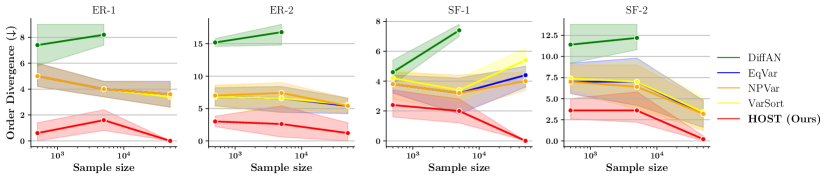
(a) Order Divergence (lower is better) with different Sample sizes.

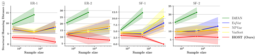
(b) Structural Hamming Distance (lower is better) with different Sample sizes.

Figure 1: Causal structure learning performance on synthetic data as function of Sample size under Linear parameterization. We fix $d=10$ and vary the sample size. The proposed HOST method is compared against DiffAN [27], EqVar [4], NPVar [10], and VarSort [23]. Column: Graph type. Shaded areas are 95% confidence intervals over five independent runs. LCIT [8] is used to recover the DAGs from the causal orders. Missing data of DiffAN is due to overly excessive runtime.

For sparse graphs, each iteration may find multiple valid source nodes. If only one is chosen then the others must have their calculations re-done multiple times, which is wasteful of resource, and the chance of miscalculation may arise in the subsequent steps as the ancestral set increases in cardinality. Therefore, we should select as many source nodes as possible in each step to avoid these pitfalls.

To do this, we employ a tolerance threshold $\epsilon$ onto the selection of the source nodes based on their $W$ statistics. Particularly, let $w^{\ast}$ be the largest $W$ statistics value of the remaining variables in each step, we will include all variables with $W$ within the $\epsilon$-radius of $w^{\ast}$ as new source nodes, which form a “layer” similarly to [10].

Further, there is a trade-off between accuracy and runtime when choosing $\epsilon$. If $\epsilon$ is too small then the effect of computation reduction is negligible, whereas larger $\epsilon$ will allow non-source nodes into the layer. In our implementation, we choose a value of $10^{-4}$, which is relatively small in comparison with the range $\left[0,1\right]$ of $W$, since accuracy is preferred in our experiments.

Of course, there can still be false positive mistakes even with small $\epsilon$ due to sampling randomness. We partially overcome this issue by adding new candidate nodes into the ancestral set in the decreasing order of their $W$ statistics. This will help ease the performance degradation for non-source nodes that are chosen into the layer but still have low $W$ statistics.

Resultantly, the causal order will be the concatenation of the layers collected after each step. Algorithm 2 summarizes the main steps of the Causal Ordering algorithm with all the technical considerations discussed.

Nevertheless, it is important to mention that our algorithm can still perform effectively even without utilizing the layer decomposition procedure. Furthermore, our layer decomposition only necessitates a single hyperparameter, the tolerance $\epsilon$. If this hyperparameter is set to zero, the feature is disabled, and this could be set as the default behavior for less experienced users of our algorithm.

3.3 DAG Recovery From the Causal Order

As stated in Lemma 2.2, one can obtain the full causal DAG from any valid causal order $\pi$. This is done by first starting with an empty DAG, then examining every ordered pair of vertices $\left(\pi_{j},\pi_{i}\right)$ to see if there is a directed edge connecting them with the help of a series of CI tests.

Alternatively, instead of CI tests, one can employ feature selection techniques with lower computational demands if runtime is preferred. For example, GAM (Generalized Additive Model) feature selection is widely used in several ordering-based methods that follow nonlinear additive noise models, e.g., [2, 25, 27]. More specifically, a GAM model is fitted to $\left(X_{\pi<i},X_{\pi_{i}}\right)$, then any significant feature $X_{\pi_{j}}$ with $j<i$, evidenced by a small $p$-value, will add an edge $\left(\pi_{j}\rightarrow\pi_{i}\right)$ to an initially empty DAG. Refer to [2] for more details on this procedure.

Finally, we put together all the pieces of our HOST method in Algorithm 3. The computational complexity of HOST is given in Appendix B, which is polynomial in both sample size and dimensionality.

4 Theoretical Properties

4.1 Identifiability of HCMs

The identifiability of HCM is given by the following Theorem.

Theorem 4.1.

Under assumptions 2.1 and 2.1, HCMs are fully identifiable, i.e., there exists a unique graph $\mathcal{G}$ consistent with data $P_{X}$ generated according to Eqn. 1.

Proof sketch.

By Lemma 3.1 a valid source node can be identified at every step, thus by induction a valid causal ordering can be identified. Then by Lemma 2.2 every true edge can be identified from the causal ordering, rendering the whole DAG identifiable. ∎

4.2 Invariance to Scaling and Translation

Another important property of our method is the invariance to scaling and invariance, which is given by the following Theorem.

Theorem 4.2.

The HOST algorithm is invariant to scaling and translation.

Proof sketch.

If we scale and translate $X_{i}$ by a scale $c>0$ and location $d$, i.e., $X^{\prime}_{i}:=cX_{i}+d$, the new causal model will have all the structural assignments and noise variables unchanged, except for $X_{i}$. Instead, we can replace it with $X^{\prime}_{i}:=\mu^{\prime}_{i}(X_{\textrm{pa}_{i}})+\sigma^{\prime}_{i}(X_{\textrm{pa}_{i}})E_{i}$, where $\mu^{\prime}_{i}:=\mu_{i}\times c+d$ and $\sigma^{\prime}_{i}:=\sigma_{i}\times c$. In case $c<0$, the negation can be absorbed to $E^{\prime}_{i}:=-E_{i}$, which is still a standard Gaussian noise mutually independent of other noises.

Note that both $\mu^{\prime}_{i}$ and $\sigma^{\prime}_{i}$ maintain the properties of $\mu_{i}$ and $\sigma_{i}$ as described in Assumption 2.1, namely being deterministic and differentiable, $\sigma^{\prime}_{i}>0$, and are non-constant with respect to any parent variable $j\in\textrm{pa}_{i}$.

Additionally, since scaling nor translation does not alter normality, Assumption 2.1 also applies to the new HCM. Consequently, the newly obtained HCM is also identifiable using our method. ∎

This property allows us to standardizing data before applying the HOST algorithm without changing the result. This is useful since neural networks, which are employed in our framework, are sensitive to data scale, meaning if the original data scale is too large or too small, the learning process may struggle to converge.

We note that this step is not possible with methods based on the “equal variance” assumption (e.g., EqVar [4] or NPVar [10]), since scaling breaks the equality between the variables’ variances, making their algorithms misbehave.

5 Numerical Evaluations

5.1 Experiment Setup

Baselines.

We evaluate both the causal ordering and causal structure learning performance of the proposed HOST method with competitive baselines in ordering-based causal structure learning, including:

VarSort [23]

simply sorts the variables according to their marginal variances based on the observation that an effect usually has higher variance than its causes in the common evaluation practice of structure learning methods on simulated data. This acts as a sanity check for the complexity of our problem.

EqVar [4]

models the data with linear relationships and homoscedastic additive noises of equal variances. At each step, the variables with minimum conditional variances given the current ancestral set are chosen as next source nodes.

NPVar [10]

extends EqVar by considering nonlinear causal mechanisms using nonparametric regression techniques. It is claimed to be able to handle heteroscedasticity, but only with constant expected noise variances, i.e., $\mathbb{E}\left[\mathbb{V}\left[X_{i}\mid X_{\mathrm{pa}_{i}}\right]\right]$.

DiffAN [27]

considers nonlinear additive noise models with homoscedastic Gaussian noises. Variables with constant partial derivatives of the score function, learned with diffusion models, are selected as sink nodes every step.

Additionally, for completeness, in Appendix C we also compare HOST with other popular baselines that are not polynomial-time, including CAM [2], GOLEM [18], and GraN-DAG [16].

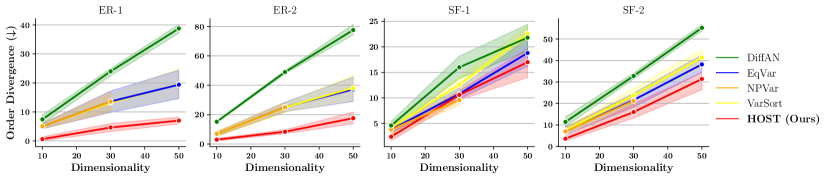
(a) Order Divergence (lower is better) with different Dimensionalities.

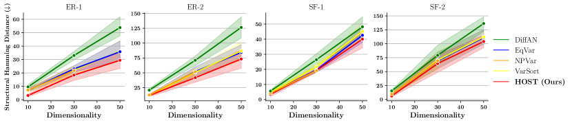
(b) Structural Hamming Distance (lower is better) with different Dimensionalities.

Figure 2: Causal structure learning performance on synthetic data as function of Dimensionality under Linear parameterization. We fix $n=500$ and vary the dimensionality. The proposed HOST method is compared against DiffAN [27], EqVar [4], NPVar [10], and VarSort [23]. Column: Graph type. Shaded areas are 95% confidence intervals over five independent runs. LCIT [8] is used to recover the DAGs from the causal orders. Missing data of NPVar is due to overly excessive runtime.

Metrics.

For assessing the causal ordering accuracy, we employ the Order Divergence measure proposed by [25], which counts the number of edges that are incorrectly ordered:

$$\text{OrderDivergence}\left(\pi,\mathcal{E}\right)=\sum_{j<i}\mathds{1}\left[\left(\pi_{i}\rightarrow\pi_{j}\right)\in\mathcal{E}\right]$$

Regarding causal structure learning, we adopt the common metric of Structural Hamming Distance, which measures the number of edge additions, removals, and reversals to transform the predicted DAG to the ground truth DAG.

In addition, to tackle scenarios where there is an imbalance between missing and extra edges, we also employ the $F_{1}$ score and AUC (Area Under the Receiver Operating Characteristic Curve) measures, which consider both false negatives and false positives. The performance of our proposed method under these metrics is provided in Appendix C, demonstrating the superiority of our proposed HOST method over the baselines in terms of both $F_{1}$ score and AUC. This finding is consistent with the results obtained using the SHD measure given in the next subsection.

DAG recovery methods.

To remove the influence of the choice of the DAG recovery method from the orderings onto the structure learning performance, we use the same algorithm for all methods. Particularly, we consider two options, first is the CI testing approach using the recent state-of-the-art test LCIT [8] since it is generic and linearly scalable in both dimensionality and sample size, along with the GAM feature selection approach which is usually employed in methods based on the equal variances assumption [2, 25, 27]. Both of them use $\alpha=0.001$.

Synthetic data.

We generate data under two typical DAG settings. First is the Erdős-Rényi (ER) graph [9], where edges are independently added with an equal probability, and we control the expected in-degree to be one (ER-1 graphs) or two (ER-2 graphs). Second is the Scale Free (SF) graph [1], with the SF-1 (SF-2) variant being the DAG initially started with one (two) nodes and every subsequent node is added with one (two) random edges from the previously added nodes. We also consider the scenarios with denser graphs (ER-4 and SF-4) in Appendix C.

About the functional mechanisms, we generate $\mu_{i}\left(\cdot\right)$ and $\sigma_{i}\left(\cdot\right)$ from the natural parametrizations and consider both linear and nonlinear scenarios. For the linear case, $\eta_{1}$ and $\ln\left(-2\eta_{2}\right)$ are homogeneous linear maps $a^{\top}x_{\mathrm{pa}_{i}}$ for each node. Meanwhile, in the nonlinear case, these parameters associated with each parent are chosen from the set $\left\{a^{\top}x,x^{2},\sin\left(2\pi x\right),\ln\left(x-\min\left(x\right)+1\right),\frac{1}{1+e^{-x}}\right\}$, and then summed afterward, e.g., $\eta_{1}\left(x_{\mathrm{pa}_{i}}\right)=\sum_{j\in\mathrm{pa}_{i}}\eta_{1}\left(x_{j}\right)$.

We emphasize here that Assumption 2.1 is not imposed in our data generating process, which means that it is possible for it to be violated in the generated data. However, even without enforcing this assumption, our method still shows robustness compared to the baselines in situations where the model is not well-specified, as evidenced by the empirical results reported in the next subsection.

5.2 Results on Synthetic Data

Here we present the empirical results for the linear parametrization setting with LCIT being the DAG recovery method. The additional experimental results, including the consideration of other evaluation metrics, nonlinear settings, GAM feature selection, denser graphs, as well as the recorded runtimes can be found in Appendix C.

Effect of sample size.

We first study the influence of sample size to the learning performance of the considering methods by fixing the number of nodes at $d=10$ and vary the sample size $n$ from 500 to 50,000 (Figure 1). The results suggest that our method is far more effective than the baseline counterparts across all scenarios, especially in the task of causal ordering. Additionally, it can be observed that our method converges to zero error on both metrics as the sample size increases, empirically suggesting its consistency.

Effect of dimensionality.

Next, we study the performance variation of all methods when the dimensionality changes. To this end, we fix the sample size at $n=500$ and vary the number of nodes from 10 to 50 (Figure 2). In this setting, while all methods show the same degradation in performance, our proposed HOST method is still the leading performer over all aspects.

Table 1: Causal structure learning performance on real data. We compare the proposed HOST with DiffAN [27], EqVar [4], NPVAR [10], and VarSort [23] on the Sachs data set [26]. The values are mean ± standard error over the same ten independent subsamples of size $700$.

	Order	Structural Hamming Distance ($\downarrow$)
	Divergence ($\downarrow$)	(CI testing)	(GAM feature selection)
DiffAN	$9.4\pm 0.70$	$15.0\pm 1.05$	$15.6\pm 0.84$
EqVar	$7.2\pm 0.42$	$\mathbf{13.5\pm 0.71}$	$\mathbf{12.0\pm 0.47}$
NPVar	$7.2\pm 0.42$	$\mathbf{13.5\pm 0.71}$	$\mathbf{12.0\pm 0.47}$
VarSort	$7.2\pm 0.42$	$13.7\pm 0.95$	$\mathbf{12.0\pm 0.47}$
HOST (Ours)	$\mathbf{4.4\pm 0.70}$	$\mathbf{13.5}\pm 0.97$	$13.3\pm 0.95$

5.3 Results on Real Data

To demonstrate the effectiveness of our method in the real-life setting, we conduct experiments on the well-known benchmark data set Sachs [26], where the ground truth causal network is available. We employ the observational portion of the data set with 853 observations, 11 vertices, and 17 edges in the causal graph.

Table 1 displays the empirical results. Our method achieves the best accuracy in recovering the causal order with an error at only half of that for other methods, while it is competitive with the state-of-the-arts in recovering the causal DAG.

6 Conclusions

This study presents the HOST algorithm for identifying the causal structures under heteroscedastic causal models. By exploiting the conditional normalities with the help of normality tests, we devise a simple procedure for recovering causal orderings, which are used to uniquely recover the causal structures. The empirical results on a wide range of synthetic and real data show that HOST is able to consistently outperform existing state-of-the-art ordering-based methods in both causal ordering and structure learning.

Appendix for “Heteroscedastic Causal Structure Learning”

A The Shapiro-Wilk Test for Normality

In the Shapiro-Wilk test, the test’s statistics is the squared correlation between the order statistics of the observations and the expected order statistics of the samples following the Gaussian distribution. More specifically, consider $n$ i.i.d. samples $\mathbf{u}_{i}=\left\{u_{i}^{\left(k\right)}\right\}_{k=1}^{n}$ of $U_{i}$. Without loss of generality, assume they are sorted, i.e., $u_{i}^{\left(k\right)}\leq u_{i}^{\left(k+1\right)}\;\forall k=1..n-1$. Similarly, let $\mathbf{Z}=\left\{Z_{k}\right\}_{k=1}^{n}$ be i.i.d. Gaussian random variables and also take their order statistics, i.e., $Z_{k}\leq Z_{k+1}\;\forall k=1..n-1$. Subsequently, define $\mathbf{m}=\left\{m_{k}=\mathbb{E}\left[Z_{k}\right]\right\}_{k=1}^{n}$ as the expectation of the order statistics.

Now, under the null hypothesis, $\mathbf{u}_{i}$ and $\mathbf{m}$ should be strongly correlated, meaning a correlation coefficient close to one would suggest $U_{i}$ is normally distributed, and a number closer to zero would indicate non-normality. The straightforward squared correlation between these two sample sets is referred to as the Shapiro-Francia statistics [28].

However, the Shapiro-Wilk statistics goes one step further as it also takes into account the covariance matrix of $Z$. More specifically, consider the covariance matrix $\Sigma$ of $Z$ where $\Sigma_{ij}=\mathbb{E}\left[\left(Z_{i}-m_{i}\right)\left(Z_{j}-m_{j}\right)\right]$ and let $\mathbf{a}=\frac{m^{\top}\Sigma^{-1}}{\left\|m^{\top}\Sigma^{-1}\right\|_{2}}$, which is a unit vector. Then, the Shapiro-Wilk test statistics is given by the squared correlation between $\mathbf{a}$ and $\mathbf{u}_{i}$:

$$W=\frac{\left(\sum_{k=1}^{n}a_{k}u_{i}^{\left(k\right)}\right)^{2}}{\sum_{k=1}^{n}\left(u_{i}^{\left(k\right)}-\bar{u_{i}}\right)^{2}}$$ (22)

B Complexity Analysis

Algorithm 1 (Latents Extraction).

With gradient-based methods such as vanilla Stochastic Gradient Ascent or Adam, the optimization process can be done in $\mathcal{O}\left(nd\right)$, with $n$ and $d$ being sample size and dimensionality, respectively. With more advanced optimizer for concave loss function, such as Newton methods or Feasible Generalized Least-squares [13], the time complexity can be furthermore reduced.

Algorithm 2 (Causal Ordering).

The main loop contains $\mathcal{O}\left(d\right)$ iterations. In each iteration, Algorithm 1 and $W$ statistics evaluation are employed $\mathcal{O}\left(d\right)$ times. To evaluate the $W$ statistics, at least $\mathcal{O}\left(n^{3}\right)$ of runtime is needed due to the inverse of $\Sigma\in\mathbb{R}^{n\times n}$, however, practical approximations for large $n$ exist and can scale very well in $n$, such as the SciPy package [36] which is used in our implementation. Additionally, sorting $L$ can be done in $\mathcal{O}\left(d\ln d\right)$ time. Assuming $n>d^{2}$ for simplicity, then Algorithm 2 operates in $\mathcal{O}\left(n^{3}d^{2}\right)$.

Algorithm 3 (HOST).

There are $\mathcal{O}\left(d^{2}\right)$ CI tests to be performed. CI tests that scale linearly with sample size and dimensionality of the conditioning set exists, e.g., [8]. Thus, the DAG recovery step can be completed in $\mathcal{O}\left(nd^{3}\right)$ runtime, so the total complexity of the HOST algorithm is $\mathcal{O}\left(nd^{2}\left(n^{2}+d\right)\right)$.

C Additional Experiments

We provide empirical results of additional settings, including:

• Figure 3 and Figure 4: We study the causal structure learning performance of HOST and competing methods under $F_{1}$ score and AUC metrics. Our method is able to outperform all baseline methods under all metrics.

• Figure 5: We study the causal structure learning performance of HOST and baselines under denser graphs settings (ER-4 and SF-4). The results, combined with those in Figure 1, suggest that as the graph density increases, all methods experience a proportional degradation in performance. However, our method still outperforms the others by a significant margin in all cases, as evidenced by the graph.

• Figure 6: We compare the runtime of all methods in the linear parametrization setting under the metric of causal ordering time, since the DAG recovery step is performed similarly with a fixed algorithm. Apart from the simple methods VarSort and EqVar which theoretically have lower computational complexities, our method is faster than both NPVar and DiffAN, except in the small sample size settings, which indicates the scalability of our method.

• Figure 7 and Figure 8: Causal structure learning performance in the linear parametrization setting with GAM feature selection as the DAG recovery method.

• Figure 9: Causal structure learning performance in the nonlinear parametrization setting with LCIT as the DAG recovery method. In this setting we use MLPs with one hidden layer of four units for $\eta_{1}$ and $\ln\left(-2\eta_{2}\right)$.

• Figure 10: We compare HOST with popular baselines that are not polynomial time, including CAM [2], GOLEM [18], and GraN-DAG [16].

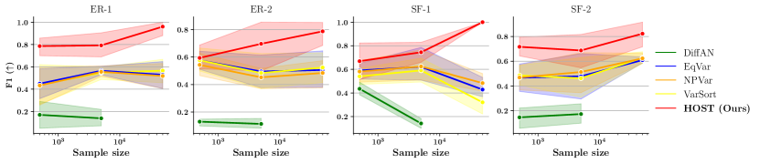
(a) $F_{1}$ score (higher is better) with different Sample sizes.

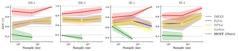
(b) AUC (higher is better) with different Sample sizes.

Figure 3: Causal structure learning performance (in $F_{1}$ score and AUC) on synthetic data as function of Sample size under Linear parameterization. We fix $d=10$ and vary the sample size. The proposed HOST method is compared against DiffAN [27], EqVar [4], NPVar [10], and VarSort [23]. Column: Graph type. Shaded areas are 95% confidence intervals over five independent runs. LCIT [8] is used to recover the DAGs from the causal orders. Missing data of NPVar is due to overly excessive runtime.

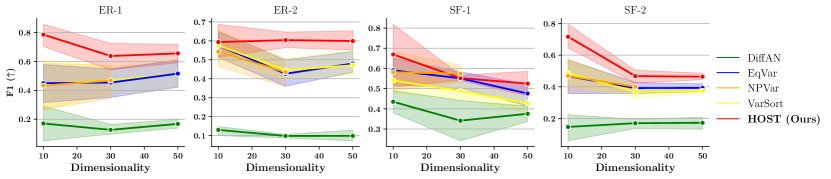
(a) $F_{1}$ score (higher is better) with different Dimensionalities.

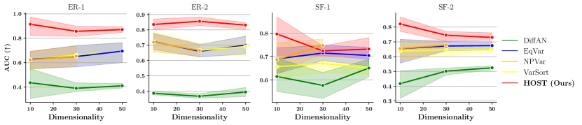
(b) AUC (higher is better) with different Dimensionalities.

Figure 4: Causal structure learning performance (in $F_{1}$ score and AUC) on synthetic data as function of Dimensionality under Linear parameterization. We fix $n=500$ and vary the dimensionality. The proposed HOST method is compared against DiffAN [27], EqVar [4], NPVar [10], and VarSort [23] under the Linear parametrization setting. Column: Graph type. Shaded areas are 95% confidence intervals over five independent runs. Missing data of NPVar is due to overly excessive runtime.

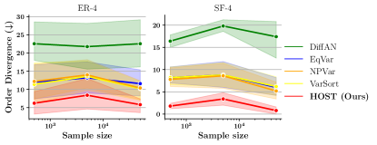
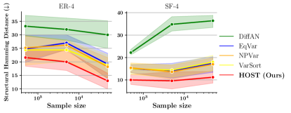
(a) Causal Ordering	(b) Causal Structure Learning

Figure 5: Causal structure learning performance on synthetic data under denser graph settings. We fix $n=5000$ and $d=10$. The proposed HOST method is compared against DiffAN [27], EqVar [4], NPVar [10], and VarSort [23] under the Linear parametrization setting. Column: Graph type. Error bars are 95% confidence intervals over five independent runs.

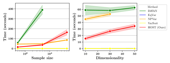
Figure 6: Causal ordering runtime. Left: we fix $d=10$ and vary the sample size; right: we fix $n=500$ and vary dimensionality. The proposed HOST method is compared against DiffAN [27], EqVar [4], NPVar [10], and VarSort [23] under the Linear parametrization setting. Shaded areas are 95% confidence intervals over five independent runs. Missing numbers of DiffAN and NPVar are due to significantly higher runtimes compared with other competitors.

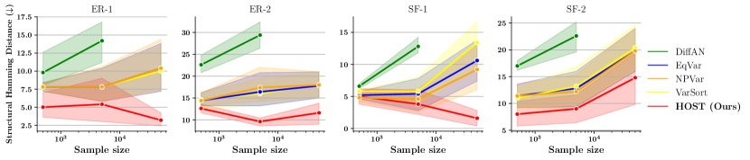
Figure 7: Causal structure learning performance on synthetic data as function of Sample size under Linear parameterization. GAM feature selection is used to recover the DAGs from the causal orders. We fix $d=10$ and vary the sample size. The proposed HOST method is compared against DiffAN [27], EqVar [4], NPVar [10], and VarSort [23]. Column: Graph type. Shaded areas are 95% confidence intervals over five independent runs. LCIT [8] is used to recover the DAGs from the causal orders.

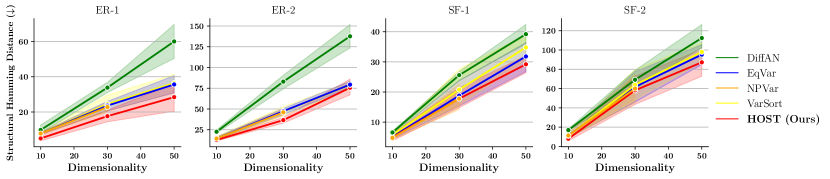
Figure 8: Causal structure learning performance on synthetic data as function of Dimensionality under Linear parameterization. GAM feature selection is used to recover the DAGs from the causal orders. We fix $n=500$ and vary the dimensionality. The proposed HOST method is compared against DiffAN [27], EqVar [4], NPVar [10], and VarSort [23]. Column: Graph type. Shaded areas are 95% confidence intervals over five independent runs.

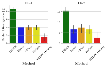
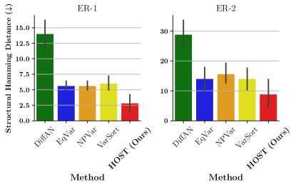
(a) Causal Ordering	(b) Causal Structure Learning

Figure 9: Causal structure learning performance on synthetic data under Nonlinear parameterization. LCIT [8] is used to recover the DAGs from the causal orders. We fix $N=5000$ and $d=10$. The proposed HOST method is compared against DiffAN [27], EqVar [4], NPVar [10], and VarSort [23]. Column: Graph type. Error bars are 95% confidence intervals over five independent runs.

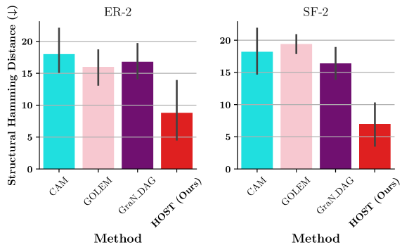
Figure 10: Causal structure learning performance on synthetic data as function of Dimensionality under Linear parameterization in comparision with non-polynomial time methods. We fix $n=500$ and $d=10$. The proposed HOST method is compared against CAM [2], GOLEM [18], and GraN-DAG [16]. Column: Graph type. Error bars are 95% confidence intervals over five independent runs.

References

- [1] Albert-László Barabási and Réka Albert, ‘Emergence of scaling in random networks’, Science, 286, 509–512, (1999).
- [2] Peter Bühlmann, Jonas Peters, and Jan Ernest, ‘Cam: Causal additive models, high-dimensional order search and penalized regression’, The Annals of Statistics, 42, 2526–2556, (2014).
- [3] Yinan Cao, Christopher Summerfield, Hame Park, Bruno Lucio Giordano, and Christoph Kayser, ‘Causal inference in the multisensory brain’, Neuron, 102, 1076–1087, (2019).
- [4] Wenyu Chen, Mathias Drton, and Y Samuel Wang, ‘On causal discovery with an equal-variance assumption’, Biometrika, 106, 973–980, (2019).
- [5] David Maxwell Chickering, ‘Optimal structure identification with greedy search’, Journal of machine learning research, 3, 507–554, (2002).
- [6] Diego Colombo, Marloes H Maathuis, Markus Kalisch, and Thomas S Richardson, ‘Learning high-dimensional directed acyclic graphs with latent and selection variables’, The Annals of Statistics, 294–321, (2012).
- [7] Keya Rani Das and AHMR Imon, ‘A brief review of tests for normality’, American Journal of Theoretical and Applied Statistics, 5, 5–12, (2016).
- [8] Bao Duong and Thin Nguyen, ‘Conditional independence testing via latent representation learning’, in Proceedings of the IEEE International Conference on Data Mining (ICDM), (2022).
- [9] Paul Erdős and Alfréd Rényi, ‘On the evolution of random graphs’, Publications of the Mathematical Institute of the Hungarian Academy of Sciences, (1960).
- [10] Ming Gao, Yi Ding, and Bryon Aragam, ‘A polynomial-time algorithm for learning nonparametric causal graphs’, in Advances in Neural Information Processing Systems, volume 33, pp. 11599–11611, (2020).
- [11] Asish Ghoshal and Jean Honorio, ‘Learning linear structural equation models in polynomial time and sample complexity’, in International Conference on Artificial Intelligence and Statistics, pp. 1466–1475, (2018).
- [12] Paul Hünermund and Elias Bareinboim, ‘Causal inference and data fusion in econometrics’, arXiv preprint arXiv:1912.09104, (2019).
- [13] Alexander Immer, Christoph Schultheiss, Julia E Vogt, Bernhard Schölkopf, Peter Bühlmann, and Alexander Marx, ‘On the identifiability and estimation of causal location-scale noise models’, arXiv preprint arXiv:2210.09054, (2022).
- [14] Dominik Janzing and Bernhard Schölkopf, ‘Causal inference using the algorithmic Markov condition’, IEEE Transactions on Information Theory, 56, 5168–5194, (2010).
- [15] Ilyes Khemakhem, Ricardo Monti, Robert Leech, and Aapo Hyvarinen, ‘Causal autoregressive flows’, in International conference on artificial intelligence and statistics, pp. 3520–3528, (2021).
- [16] Sébastien Lachapelle, Philippe Brouillard, Tristan Deleu, and Simon Lacoste-Julien, ‘Gradient-based neural dag learning’, in International Conference on Learning Representations, (2020).
- [17] Quoc V Le, Alex J Smola, and Stéphane Canu, ‘Heteroscedastic gaussian process regression’, in Proceedings of the 22nd international conference on Machine learning, pp. 489–496, (2005).
- [18] Ignavier Ng, AmirEmad Ghassami, and Kun Zhang, ‘On the role of sparsity and dag constraints for learning linear dags’, Advances in Neural Information Processing Systems, 17943–17954, (2020).
- [19] Goutham Rajendran, Bohdan Kivva, Ming Gao, and Bryon Aragam, ‘Structure learning in polynomial time: Greedy algorithms, bregman information, and exponential families’, in Advances in Neural Information Processing Systems, volume 34, pp. 18660–18672, (2021).
- [20] Joseph Ramsey, Madelyn Glymour, Ruben Sanchez-Romero, and Clark Glymour, ‘A million variables and more: the Fast Greedy Equivalence Search algorithm for learning high-dimensional graphical causal models, with an application to functional magnetic resonance images’, International Journal of Data Science and Analytics, 3, 121–129, (2017).
- [21] Joseph D Ramsey, ‘Scaling up greedy causal search for continuous variables’, arXiv preprint arXiv:1507.07749, (2015).
- [22] Nornadiah Mohd Razali, Yap Bee Wah, et al., ‘Power comparisons of shapiro-wilk, kolmogorov-smirnov, lilliefors and anderson-darling tests’, Journal of statistical modeling and analytics, 2, 21–33, (2011).
- [23] Alexander Reisach, Christof Seiler, and Sebastian Weichwald, ‘Beware of the simulated dag! causal discovery benchmarks may be easy to game’, in Advances in Neural Information Processing Systems, volume 34, pp. 27772–27784, (2021).
- [24] Robert W Robinson, ‘Counting unlabeled acyclic digraphs’, in Combinatorial Mathematics V, 28–43, Springer, (1977).
- [25] Paul Rolland, Volkan Cevher, Matthäus Kleindessner, Chris Russell, Dominik Janzing, Bernhard Schölkopf, and Francesco Locatello, ‘Score matching enables causal discovery of nonlinear additive noise models’, in International Conference on Machine Learning, pp. 18741–18753, (2022).
- [26] Karen Sachs, Omar Perez, Dana Pe’er, Douglas A Lauffenburger, and Garry P Nolan, ‘Causal protein-signaling networks derived from multiparameter single-cell data’, Science, 308, 523–529, (2005).
- [27] Pedro Sanchez, Xiao Liu, Alison Q O’Neil, and Sotirios A. Tsaftaris, ‘Diffusion models for causal discovery via topological ordering’, in The Eleventh International Conference on Learning Representations, (2023).
- [28] Samuel S Shapiro and RS Francia, ‘An approximate analysis of variance test for normality’, Journal of the American statistical Association, 67, 215–216, (1972).
- [29] Samuel Sanford Shapiro and Martin B Wilk, ‘An analysis of variance test for normality (complete samples)’, Biometrika, 52, 591–611, (1965).
- [30] Peter Spirtes and Clark Glymour, ‘An algorithm for fast recovery of sparse causal graphs’, Social Science Computer Review, 9, 62–72, (1991).
- [31] Peter Spirtes, Clark N Glymour, Richard Scheines, and David Heckerman, Causation, prediction, and search, MIT Press, 2000.
- [32] Chandler Squires and Caroline Uhler, ‘Causal structure learning: A combinatorial perspective’, arXiv preprint arXiv:2206.01152, (2022).
- [33] Eric V Strobl and Thomas A Lasko, ‘Identifying patient-specific root causes with the heteroscedastic noise model’, arXiv preprint arXiv:2205.13085, (2022).
- [34] Henry C Thode, Testing for normality, CRC press, 2002.
- [35] Thomas Verma and Judea Pearl, ‘Causal networks: Semantics and expressiveness’, in Machine intelligence and pattern recognition, volume 9, 69–76, Elsevier, (1990).
- [36] Pauli Virtanen, Ralf Gommers, Travis E Oliphant, Matt Haberland, Tyler Reddy, David Cournapeau, Evgeni Burovski, Pearu Peterson, Warren Weckesser, Jonathan Bright, et al., ‘Scipy 1.0: fundamental algorithms for scientific computing in python’, Nature methods, 17, 261–272, (2020).
- [37] Sascha Xu, Osman A Mian, Alexander Marx, and Jilles Vreeken, ‘Inferring cause and effect in the presence of heteroscedastic noise’, in International Conference on Machine Learning, pp. 24615–24630, (2022).
- [38] Xun Zheng, Bryon Aragam, Pradeep Ravikumar, and Eric P. Xing, ‘DAGs with NO TEARS: Continuous optimization for structure learning’, in Advances in Neural Information Processing Systems, pp. 9472–9483, (2018).
- [39] Xun Zheng, Chen Dan, Bryon Aragam, Pradeep Ravikumar, and Eric P. Xing, ‘Learning sparse nonparametric dags’, in Proceedings of the International Conference on Artificial Intelligence and Statistics, (2020).