Dual-level Interaction for Domain Adaptive Semantic Segmentation

Abstract

Self-training approach recently secures its position in domain adaptive semantic segmentation, where a model is trained with target domain pseudo-labels. Current advances have mitigated noisy pseudo-labels resulting from the domain gap. However, they still struggle with erroneous pseudo-labels near the boundaries of the semantic classifier. In this paper, we tackle this issue by proposing a dual-level interaction for domain adaptation (DIDA) in semantic segmentation. Explicitly, we encourage the different augmented views of the same pixel to have not only similar class prediction (semantic-level) but also akin similarity relationship with respect to other pixels (instance-level). As it’s impossible to keep features of all pixel instances for a dataset, we, therefore, maintain a labeled instance bank with dynamic updating strategies to selectively store the informative features of instances. Further, DIDA performs cross-level interaction with scattering and gathering techniques to regenerate more reliable pseudo-labels. Our method outperforms the state-of-the-art by a notable margin, especially on confusing and long-tailed classes. Code is available at https://github.com/RainJamesY/DIDA

1 Introduction

Semantic segmentation, aiming at assigning a label for every single pixel in a given image, is a fundamental task in computer vision.Learning with synthetic data (e.g., from virtual simulation [30] or open-world games [29]) has revolutionized segmentation tasks over the past few years, which effectively saves time and labor from the onerous pixel-level annotations. However, the existence of domain shifts between the rendered synthetic data and real-world distributions severely reduces the models’ performance [48]. To mitigate this problem, Unsupervised Domain Adaptation (UDA) is explored to generalize the network trained with labeled source (synthetic) data to unlabeled target (real) data.

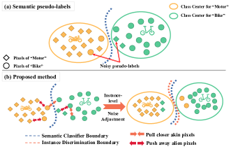
Figure 1: Intuition behind DIDA. (a) The semantic classifier trained on the source domain can be viewed as class feature centers, which possess a natural weakness in classifying pixels near or across the category boundaries thus producing erroneous and noisy semantic pseudo-labels. (b) In DIDA, we utilize instance-level discrimination with proposed instance loss to adjust noisy pseudo-labels. By simultaneously considering the semantic-level and instance-level information with cross-level interaction, we reset the classification boundaries for more robust pseudo-labeling.

Existing Work: Most of the existing works on self-training UDA [49, 37, 48] generate target domain pseudo-labels based on the semantic-level class predictions of the network for future self-training. To step further, a very recent work DAFormer [14] utilizes a Transformer encoder and a multilevel feature fusion decoder architecture, and designed three training strategies to stabilize training as well as avoid overfitting, which achieved state-of-the-art performance.

One problem of the existing methods is that they still preserve a large number of noisy pseudo-labels, especially those near the decision boundaries (Figure 1(a)). This is because they only obtain the pseudo-labels through the semantic classifier and eliminate the unreliable pseudo-labels via selecting a confidence threshold, which is rather an empirical process varying across tasks, models, and datasets [50]. It is extremely difficult to formulate such selection as a mathematical function, making it hard to optimize. Furthermore, the presence of confusing (e.g., analogous and adjacent/overlapping) categories leads to an open issue known as “overconfidence” [49], which significantly degrades the performance on these categories (Table 1 and 2).

Our Work: To alleviate the aforementioned limitations, in this paper, we propose to leverage Dual-level Interaction for Domain Adaptive (DIDA) semantic segmentation. Inspired by previous work [32] that the fine-grained instance-level discrimination could be conducive to adjusting noisy semantic-level pseudo-labels, especially those around classifier boundaries, in DIDA, we simultaneously consider the semantic-level and instance-level consistency regularization. Specifically, we encourage different (weakly and strongly) augmented views of the same pixel to have not only consistent semantic class prediction but also akin similarity relationship towards other pixels (instance-level discrimination) to provide additional instance-feature consistency beyond the semantics. As a result, we adjust the distribution of semantic pseudo-labels with proposed instance loss and reset the classification boundaries (Figure 1(b)).

In the semantic segmentation task, the main challenge of introducing instance-level discrimination is that features of pixel instances (instead of image-wise instances in classification tasks ) can cause tremendous extra storage (e.g., 50 billion instances for the GTA5 dataset). To overcome this issue, we design a labeled Instance Bank (IB) to selectively deposit instance features rather than keeping the entirety. We dynamically update our IB via our class-balanced sampling (CBS) and boundary pixel selecting (BPS) strategies. By doing so, DIDA enriches the fine-grained instance-level pseudo-labels with long-tailed and analogous categories for future self-training, and thus the model becomes more at ease in dealing with such tricky categories. Different from previous methods that naively calculate on semantic pseudo-labels [37, 48, 14] or incorporate instance information by simply adding loss components [21, 22, 40], we further present scattering and gathering techniques to interact predictions from both levels, thus generating less noisy training targets.

Considering the strong similarity among fine-grained computer vision tasks, our framework shows prominent applicability to other self-training scenarios.

Our key contributions are summarized as follows:

• We propose DIDA, a novel framework that exploits both semantic-level and instance-level consistency regularization for better noise adjustment. To the best of our knowledge, in the task of UDA for semantic segmentation, we are the first attempt that allows the information (the pseudo-labels) of two levels to calibrate and interact with each other.

• We design a labeled instance bank to overcome the issue of storage in incorporating the instance-level information and devise class-balanced sampling and boundary pixel selecting strategies to enhance the performance on long-tailed and analogous categories.

• The proposed DIDA notably outperforms the previous state-of-the-art. On GTA5 $\rightarrow$ Cityscapes adaptation, we improve the mIoU from 68.3 to 71.0 and on SYNTHIA $\rightarrow$ Cityscapes from 60.9 to 63.3. Especially, DIDA shows outstanding IoU results on the confusing classes such as “sidewalk” and “truck” as well as long-tailed classes such as “train” and “sign”.

2 Related Work

Domain Adaptation for semantic segmentation. Multiple methods have been proposed to bridge the domain gap between synthetic data and real ones. Compared to adversarial training methods that align distributions of source and target domain at different levels, i.e., input-level [33, 12], feature-level [13, 3], and output-level [41, 39], the self-training approaches obtain more competitive results. By generating target domain pseudo-labels and iteratively refining (self-training) the model using the most confident ones [1, 15, 20, 50], the model’s performance is further improved. However, the naive generation of target domain pseudo-labels is error-prone, causing the network to converge in the wrong direction. Therefore, several works were proposed to “rectify” the erroneous pseudo-labels on the semantic-level [18, 44, 17, 34]. Following this trend, DACS [37] used data-augmented consistency regularization [2] to mix source and target images during training. ProDA [48] employed correction of pseudo-labels with feature distances to prototypes. Lukas et al. [14] referred to the UDA strategy from DACS [37] and demonstrated state-of-the-art performance using Transformer as the backbone. There also exist works that exploit instance information, for example, Liu et al. devised a patch-wise contrastive learning framework, BAPA-Net [22] encouraged prototype alignment at the class-level, CLUDA [40] incorporated contrastive loss using target domain semantic pseudo-labels. However, the above methods either solely focused on semantic pseudo-label rectification or naively incorporated instance information by additional loss components. In contrast, our method introduces instance consistency regularization as an auxiliary classifier to produce pseudo-labels with different noisy patterns and further adjusts pseudo-labels of the two levels with interactive techniques.

Consistency Regularization. Consistency Regularization is first explored in Semi-supervised Learning (SSL) [2, 35] and is recently adapted to Unsupervised Domain Adaptation (UDA) [47, 25, 7, 28]. The core idea of Consistency Regularization is to encourage the model to produce similar output predictions for the same input/feature with different perturbations, e.g., the input perturbation methods [6, 47] randomly augment the input images with different augmentation degree and the feature perturbation [26, 16] is generally applied by using multiple decoders and supervising the consistency between the outputs of different decoders. Since our dual-level interaction method mainly explores the intrinsic pixel structures of an image, we optimize our model from a batch of differently augmented target input. Moreover, recent advances [23, 37, 25] concluded that the Cross-Entropy (CE) loss performs better in the fine-grained segmentation task than the Mean Square Error (MSE) loss and Kullback-Leibler (KL) loss. Therefore, in this work, we adopt the CE loss to enforce the consistency of instance-level discrimination.

3 Method

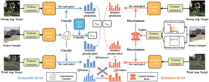
Figure 2: Overview of DIDA framework. The black stream of data augmentation and feature extraction process produces feature maps from an identical batch of input images. The blue and red streams are the semantic-level and instance-level self-training process, respectively, which can be viewed as consistency regularization on both levels produce the $\mathcal{L}_{tgt}$ and $\mathcal{L}_{ins}$. DIDA adopts class-balanced sampling (CBS) and boundary pixel selecting (BPS) to filter useful source instance features and deposit them into the labeled instance bank (IB) (Sec. 3.4). We use the source instance features (stored in IB) as the “instance classifier” and discriminate between source and target instances to produce instance pseudo-labels (Sec. 3.2). The pseudo-label regeneration (bottom middle) calibrates pseudo-labels from the two levels (with different channel sizes), then regenerates less noisy pseudo-labels to replace the naive ones (Sec. 3.3). During each iteration, the source domain training process of $\mathcal{L}_{src}$ and the self-training process of two levels start simultaneously and obtain the summed overall training objective $\mathcal{L}_{overall}$.

3.1 Preliminaries

In this section, we introduce the preliminary semantic-level self-training method for UDA [50, 37, 14]. Given the source domain images $\mathcal{X}_{s}=\left\{x_{s}\right\}_{j=1}^{n_{s}}$ with segmentation labels $\mathcal{Y}_{s}=\left\{y_{s}\right\}_{j=1}^{n_{s}}$, a neural network is trained to obtain useful knowledge from the source and is expected to achieve good performance on the target images $\mathcal{X}_{t}=\left\{x_{t}\right\}_{j=1}^{n_{t}}$ without the target ground truth labels. In the following sections, we use $i$ to note the $i$-th pixel in an image and $j$ to note the $j$-th image sample in datasets from each domain.

In a typical UDA pipeline, we first train a neural network $h$ with labeled source data. The network $h$ can be divided into $h=f\circ g$, where $f(\cdot)$ is a feature extractor that extracts a feature map $\mathbf{m}=f(x_{s})$ from a given source image $x_{s}$, and $g(\cdot)$ is the fully connected pixel level classifier which is employed to map $\mathbf{m}$ into semantic predictions, written as $p_{s}=g(\mathbf{m})$. Afterward, the source domain samples are directly optimized with a categorical cross-entropy (CE) loss:

$$\mathcal{L}_{src}=-\sum_{i=1}^{H\times W}\sum_{c=1}^{C}y_{s}^{(i,c)}\log(p_{s}^{(i,c)}),$$ (1)

where $p_{s}^{(i,c)}$ represents the softmax probability of pixel $x_{s}^{(i)}$ belonging to the $c$-th class. A similar definition applies to $p_{t}^{(i,c)}$. Since the naive network $h=f\circ g$ trained with source data does not generalize well to the target domain owing to the domain gap, the self-training approaches first assign semantic pseudo-labels to the images from the target domain and then train $h$ with the pseudo-labeled images. A conventional method is to use the most probable class predicted by $h$ as the semantic pseudo-labels: small

$$\hat{y}_{t}^{(i,c)}=\left\{\begin{array}[]{ll}1,&\textrm{if}\quad c=\underset{c^{\prime}}{\arg\max}\,p_{t}^{\left(i,c^{\prime}\right)},\\ 0,&\textrm{otherwise}\end{array}\right.$$ (4)

Evidently, this “brute force” strategy suffers from the noisy-label problem [37, 48]. This is because the pixels near the decision boundary are likely to be assigned with wrong pseudo-labels. A typical method to mitigate this problem is to set a confidence threshold $\tau$ to filter target sample pixels whose largest class probabilities in the pseudo-labels are larger than $\tau$ [37, 14]. In this way, the unsupervised semantic-level classification loss on the target domain can be defined as:

$$\mathcal{L}_{tgt}=-\sum_{i=1}^{H\times W}\sum_{c=1}^{C}\mathbbm{1}\left(\max\,\hat{y}_{t}^{(i,c)}>\tau\right)\log(p_{t}^{(i,c)}).$$ (5)

Unfortunately, an open problem of the existing threshold-based methods is that it is extremely difficult to find a “perfect” threshold that can exclude all noisy labels. This is because the selection of threshold is rather an empirical process [50], which varies between tasks and datasets. Thus it is challenging to formulate it as a general mathematical function, making this problem hard to optimize. In this paper, we address this problem from a totally different viewpoint: seeking the regularization of the semantic pseudo-labels from the instance-level perspective.

3.2 Instance-Level Discrimination

For this component, we view each pixel instance as a distinct class of its own and adjust our model to distinguish between “individual” instance classes.

Firstly, we generate the source domain image-wise feature map $\mathbf{m}_{s}\in\mathbf{R}^{[H\times W]\times D}$ ($D$ is the channel size of the extracted feature). Noticeably, $\mathbf{m}_{s}$ consists of $H\times W$ corresponding pixels, and each pixel possesses an embedding $e_{s}$ with shape $[1\times 1]\times D$, $e_{s}\in\mathbf{m}_{s}$. As mentioned earlier, it is impossible to store all extracted pixel-level features in the memory, thus we selectively store some of them in the memory bank $\mathcal{B}$ (see updating strategy in Sec. 3.4). We denote the embeddings of pixels deposited in the bank $\mathcal{B}$ (obtained from source domain image) as $\left\{e_{k}:k\in(1,\ldots,K)\right\}$. Likewise, $\mathbf{m}^{A}_{t}$ and $\mathbf{m}_{t}^{\alpha}$ are feature maps obtained from strongly-augmented and weakly augmented target samples, where $e^{A}_{t}\in\mathbf{m}^{A}_{t}$ and $e_{t}^{\alpha}\in\mathbf{m}_{t}^{\alpha}$ are used to represent instance embeddings. The source domain features in the bank serve as our auxiliary “instance classifier” that goes beyond the limitation of the semantic decision boundary.

Under the non-parametric softmax formulation [45], for strongly augmented target pixel instance $x_{t}^{A(i)}$ with embedding $e^{A}_{t}$, we use the $cosine$ $similarity$ $\mathbf{cos\_sim}(\mathbf{u},\mathbf{v})=\mathbf{u}^{T}\mathbf{v}/\|\mathbf{u}\|\|\mathbf{v}\|$ to calculate its instance-level similarity with each sample in $\mathcal{B}$, as the instance-level prediction of $x_{t}^{A(i)}$:

$$\hat{y}_{ins}^{(i)} =[q_{1}^{A},\dots,q_{k^{\prime}}^{A},\dots]$$ (6)

where $$\quad q_{k^{\prime}}^{A}=\frac{\exp\left((e_{t}^{A})^{T}e_{k^{\prime}}/tp\right)}{\sum_{k=1}^{K}\exp\left((e_{t}^{A})^{T}e_{k}/tp\right)},$$

where $tp$ is temperature, a hyperparameter that controls the flatness of the distribution. This equation measures the probability of target pixel-level instance $x_{t}^{(i)}$ being recognized as $k^{\prime}$-th source instance in our memory bank $\mathcal{B}$, acting as “discriminate” in Figure 2. A similar calculation from the weakly augmented pixel-level sample $x_{t}^{\alpha(i)}$ can be defined as the instance-level pseudo-label:

$${y}_{ins}^{(i)}=[q_{1}^{\alpha},\dots,q_{k^{\prime}}^{\alpha},\dots],$$ (7)

$$\textrm{where}\quad q_{k^{\prime}}^{\alpha}=\frac{\exp\left((e_{t}^{\alpha})^{T}e_{k^{\prime}}/tp\right)}{\sum_{k=1}^{K}\exp\left((e_{t}^{\alpha})^{T}e_{k}/tp\right)},$$

Then, this naive instance-level pseudo-label will be used to adjust the semantic-level pseudo-label during the following pseudo-label regeneration process. Finally, an additional CE loss function is then introduced to minimize the difference between $\hat{y}_{ins}^{(i)}$ and ${y}_{ins}^{(i)}$:

$$\mathcal{L}_{ins}=-\sum_{i=1}^{H\times W}{y}_{ins}^{(i)}\log\left(\hat{y}_{ins}^{(i)}\right)$$ (8)

Finally, our overall UDA objective $\mathcal{L}_{overall}$ is calculated as the weighted sum of each loss component as $\mathcal{L}_{{overall}}=\mathcal{L}_{src}+\mathcal{L}_{tgt}+\lambda_{ins}\mathcal{L}_{ins}$ , where $\lambda_{ins}$ is the parameter controlling the weight of instance loss.

3.3 Pseudo-label Regeneration

As we mentioned earlier, the naive semantic-level pseudo-labels are glutted with noises. To further improve the quality of the pseudo-labels, we creatively propose the pseudo-label regeneration to exhaustively utilize the labeled information and introduce a way to calibrate semantic predictions and instance predictions so that they could interact with and adjust each other. During the regeneration, our key objective is to align the semantic-level and instance-level predictions which possess different channel sizes.

For an input weakly augmented target image $x^{\alpha}_{t}$ (bottom row of Figure 2), we first extract its image-wise feature map $\mathbf{m}^{\alpha}_{t}$, then we obtain its semantic predictions using our pixel-level classifier $p^{\alpha}_{t}=g(\mathbf{m}^{\alpha}_{t})$, $p^{\alpha}_{t}\in\mathbf{R}^{[H\times W]\times C}$. For a single pixel within $\mathbf{m}^{\alpha}_{t}$, we denote its semantic prediction as $z^{t}\in\mathbf{R}^{[1\times 1]\times C}$ and calculate its instance-level similarity predictions via Eq. (7) as $q^{\alpha}\in\mathbf{R}^{[1\times 1]\times K}$ . Generally, $K$ is much larger than $C$ since at least one instance is needed for each semantic category. We then calibrate $z^{t}$ with $q^{\alpha}$ by scattering $z^{t}$ into $K$ dimensional space, denoted as $z^{sc}\in\mathbf{R}^{[1\times 1]\times K}$

$$z_{k}^{sc}=z_{j}^{t},\text{ if }{label}\left(q_{k}^{\alpha}\right)={label}\left(z_{j}^{t}\right),$$ (9)

where $label(\cdot)$ is the function that returns the ground truth label. For example, $label(q_{k}^{\alpha})$ means the label for the $k^{th}$ element in the instance bank and ${label}\left(z_{j}^{t}\right)$ stands for the $j^{th}$ semantic category for the “softmaxed” prediction.

The regeneration of instance pseudo-labels is expressed as the scaling between new and old instance-level predictions:

$$\hat{q}_{k}=\frac{q_{k}^{\alpha}z_{k}^{sc}}{\sum_{k=1}^{K}q_{k}^{\alpha}z_{k}^{{sc}}}.$$ (10)

We adopt the newly calibrated $\hat{q}$ to replace the old ${y}_{ins}$ in Eq.(8).

Furthermore, to interact the semantic-level with instance information, we gather $q$ into $C$ dimensional space by summing over instance predictions with shared labels

$$q_{i}^{ga}=\sum_{j=0}^{K}\mathbbm{1}\left({label}\left(z_{i}^{t}\right)={label}\left(q_{j}^{\alpha}\right)\right)q_{j}^{\alpha}$$ (11)

Now we may further adjust the semantic pseudo-label by smoothing $z^{t}$ with $q^{ga}$, written as:

$$\hat{z}_{i}=\phi z_{i}^{t}+(1-\phi)q_{i}^{ga},$$ (12)

where $\phi$ is a hyper-parameter that balances the weight of semantic and instance information. Similarly, the adjusted $\hat{z}$ will replace the old semantic pseudo-label $\hat{y}_{t}$ in Eq. (5). Note that the pseudo-regeneration of two levels starts simultaneously since we use copies of old ${y}_{ins}$ and $\hat{y}_{t}$ for regeneration. By doing so, the dual-level information is subtly interacted with and follows the protocol that the distributions of two levels are always expected to agree with each other, as illustrated in Figure 3.

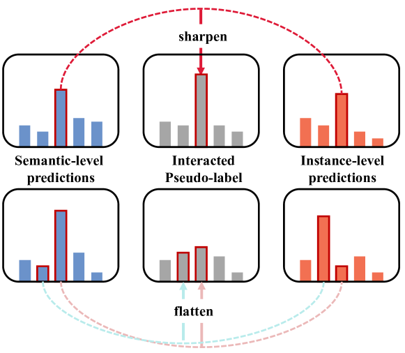
Figure 3: Intuition behind pseudo-label regeneration. After we calibrate the predictions obtained from the two levels, we compare the highest possibility in each level. If the most possible predictions are similar within the two levels, the regenerated pseudo-label will become sharper in the most confident category. In contrast, if the predictions of two levels disagree with each other, they will check and balance the interacted pseudo-labels, resulting in a much flatter distribution.

3.4 Instance Bank and Updating Strategies

As mentioned above, with designed bank size $K$ and embedding size $D$, we construct a feature bank $\mathcal{B}_{f}\in\mathbf{R}^{K\times D}$ and a label bank $\mathcal{B}_{l}\in\mathbf{R}^{K\times 1}$ to keep instance-level information: the extracted instance embeddings and their corresponding ground truth labels. Different from domain adaptation for classification where features of all images can be stored, for the segmentation task, we strictly control the bank size and meticulously scheme its updating strategies.

Our key observation which motivates us to carefully design the updating strategy is that the long-tailed class distribution of source data (see supplementary material for details) will result in a strong bias towards common classes (e.g., “road”, “sky”) instead of classes with very limited pixels (e.g., “sign”, “light”) and those only appear in a few samples (e.g., “bike”, “rider”). In addition, most pixels of an entity are actually redundant and less determinant to the segmentation performance than those around object boundaries. To address these two issues and make the deposited instance feature embeddings more representative, we proposed two strategies, i.e., class-balanced sampling and boundary pixel selecting.

Class-Balanced Sampling (CBS). Before saving instance-level embeddings to $\mathcal{B}$, we set the same proportions of labeled place-holders for each class, i.e., $Holders=\frac{K}{C}$. The feature bank is initiated offline with randomly selected instance embeddings but updated online through our selecting strategies. We have also experimented with different bank sizes $K$ and different distributions of classes within, please see more details in our experiment and analysis (Sec. 4.3).

Boundary Pixel Selecting (BPS). We first generate boundary masks $\mathcal{M}_{s}$ for each annotated source sample through Algorithm 1, then the boundary pixel maps $\mathcal{E}_{s}$ are easily calculated by $\mathcal{Y}_{s}*\mathcal{M}_{s}$.

Input : Ground truth label $\mathcal{Y}_{s}^{l}$ of size $H\times W$

Output : Boundary mask $\mathcal{M}_{l}$ of image $l$

Initialization: All-zero matrix $\mathcal{M}_{l}$ of size $H\times W$, receptive field $R$ of size $3\times 3$, threshold $\sigma\leftarrow 2$

for $i\leftarrow 0$ to $H$ do

       for $j\leftarrow 0$ to $W$ do

             Initiate $ClassCount\leftarrow 0$

            $Current\leftarrow$ pixel $\mathcal{Y}[i,j]$ ($Current$ is the position of current pixel)

            $ClassCount$ $\leftarrow$ Count of different classes within $Current$ receptive field $R$

            if $ClassCount>\sigma$ then

                   $\mathcal{M}[i,j]\leftarrow 1$

            

      

Algorithm 1 Boundary Mask Generation

For the $c$-th class, we take the average of embeddings matching $\mathcal{E}_{s}^{c}$ as $emb_{b}^{c}$. To balance our selection, we adopt K-means clustering [24] on the non-edge instances and pick out the centroid embeddings $emb_{\theta}^{c}$ of the $c$-th cluster. Together, the averaged instance feature embeddings $emb^{avg}\in\mathbf{R}^{1\times C}$ between $emb_{b}$ and $emb_{\theta}$ are what we need to update the feature bank during each update interval $u$ with ema smoothing [36]:

$$emb_{u}\leftarrow\omega\cdot{emb}_{u-1}+(1-\omega)emb^{avg}$$ (13)

Here $\omega$ $\in$ [0, 1) is a momentum coefficient. Unlike ProDA [48] which calculates target domain prototypes on the semantic pseudo-labels, our BPS obtains more representative source domain prototypes to perform instance-level discrimination. Particularly, if the current image does not contain a certain class of instances, we skip updating all embeddings belonging to this class for once.

4 Experiments

Table 1: Comparison with state-of-the-art (SOTA) methods for UDA from GTA5 [29] $\rightarrow$ Cityscapes [5] adaptation. The results for DIDA are averaged over 3 random seeds. ^† means we report the ProDA [48] and CPSL [19] results without further distillation for fair comparison. Noted that we use gray to highlight 9 long-tailed classes, and symbols [^⋆∘∙] stand for analogous pairs. The best and second-best results are highlighted in bold and underline font, respectively.

Method

Venue

Road⋆

S.walk⋆

Build.

Wall

Fence

Pole

Light

Sign

Veget.

Terrain

Sky

Person

Rider

Car

Truck∘

Bus∘

Train

motor∙

Bike∙

mIoU

GTA5 $\rightarrow$ Cityscapes

DACS [37]	WACV’21	89.9	39.7	87.9	30.7	39.5	38.5	46.4	52.8	88.0	44.0	88.8	67.2	35.8	84.5	45.7	50.2	0.0	27.3	34.0	52.1
BiMAL [38]	ICCV’21	91.2	39.6	82.7	29.4	25.2	29.6	34.3	25.5	85.4	44.0	80.8	59.7	30.4	86.6	38.5	47.6	1.2	34.0	36.8	47.3
UncerDA [43]	ICCV’21	90.5	38.7	86.5	41.1	32.9	40.5	48.2	42.1	86.5	36.8	84.2	64.5	38.1	87.2	34.8	50.4	0.2	41.8	54.6	52.6
BAPA-Net [22]	ICCV’21	94.4	61.0	88.0	26.8	39.9	38.3	46.1	55.3	87.8	46.1	89.4	68.8	40.0	90.2	60.4	59.0	0.00	45.1	54.2	57.4
DPL-Dual [4]	ICCV’21	92.8	54.4	86.2	41.6	32.7	36.4	49.0	34.0	85.8	41.3	86.0	63.2	34.2	87.2	39.3	44.5	18.7	42.6	43.1	53.3
UPLR [42]	ICCV’21	90.5	38.7	86.5	41.1	32.9	40.5	48.2	42.1	86.5	36.8	84.2	64.5	38.1	87.2	34.8	50.4	0.2	41.8	54.6	52.6
ProDA† [48]	CVPR’21	91.5	52.4	82.9	42.0	35.7	40.0	44.4	43.3	87.0	43.8	79.5	66.5	31.4	86.7	41.1	52.5	1.0	45.4	53.8	53.7
SAC [1]	CVPR’21	90.4	53.9	86.6	42.4	27.3	45.1	48.5	42.7	87.4	40.1	86.1	67.5	29.7	88.5	49.1	54.6	9.8	26.6	45.3	53.8
CPSL† [19]	CVPR’22	91.7	52.9	83.6	43.0	32.3	43.7	51.3	42.8	85.4	37.6	81.1	69.5	30.0	88.1	44.1	59.9	24.9	47.2	48.4	55.7
CaCo [15]	CVPR’22	93.8	64.1	85.7	43.7	42.2	46.1	50.1	54.0	88.7	47.0	86.5	68.1	2.9	88.0	43.4	60.1	31.5	46.1	60.9	58.0
DAFormer [14]	CVPR’22	95.7	70.2	89.4	53.5	48.1	49.6	55.8	59.4	89.9	47.9	92.5	72.2	44.7	92.3	74.5	78.2	65.1	55.9	61.8	68.3
DIDA (Ours)	–	97.3	78.0	89.8	55.9	52.6	53.3	57.9	66.1	90.0	50.0	93.1	73.2	44.8	93.4	80.9	84.7	73.8	58.6	63.5	71.0

Table 2: Comparison with state-of-the-art (SOTA) methods from SYNTHIA [30] $\rightarrow$ Cityscapes [5] adaptation. mIoU* denotes the mean IoU over 13 classes excluding “wall”, “fence”, and “pole”.

Method

Venue

Road⋆

S.walk⋆

Build.

Wall

Fence

Pole

Light

Sign

Veget.

Sky

Person

Rider

Car

Bus

motor∙

Bike∙

mIoU

mIoU*

SYNTHIA $\rightarrow$ Cityscapes

DACS [37]	WACV’21	80.6	25.1	81.9	21.5	2.9	37.2	22.7	24.0	83.7	90.8	67.6	38.3	82.9	38.9	28.5	47.6	48.3	54.8
BiMAL [38]	ICCV’21	92.8	51.5	81.5	10.2	1.0	30.4	17.6	15.9	82.4	84.6	55.9	22.3	85.7	44.5	24.6	38.8	46.2	53.7
UncerDA [43]	ICCV’21	79.4	34.6	83.5	19.3	2.8	35.3	32.1	26.9	78.8	79.6	66.6	30.3	86.1	36.6	19.5	56.9	48.0	54.6
BAPA-Net [22]	ICCV’21	91.7	53.8	83.9	22.4	0.8	34.9	30.5	42.8	86.6	88.2	66.0	34.1	86.6	51.3	29.4	50.5	53.3	61.2
DPL-Dual [4]	ICCV’21	83.5	38.2	80.4	1.3	1.1	29.1	20.2	32.7	81.8	83.6	55.9	20.3	79.4	26.6	7.4	46.2	43.0	50.5
UPLR [42]	ICCV’21	79.4	34.6	83.5	19.3	2.8	35.3	32.1	26.9	78.8	79.6	66.6	30.3	86.1	36.6	19.5	56.9	48.0	54.6
ProDA† [48]	CVPR’21	87.3	44.0	83.2	26.9	0.7	42.0	45.8	34.2	86.7	81.3	68.4	22.1	87.7	50.0	31.4	38.6	51.9	62.0
SAC [1]	CVPR’21	89.3	47.2	85.5	26.5	1.3	43.0	45.5	32.0	87.1	89.3	63.6	25.4	86.9	35.6	30.4	53.0	52.6	59.3
CPSL† [19]	CVPR’22	87.3	44.4	83.8	25.0	0.4	42.9	47.5	32.4	86.5	83.3	69.6	29.1	89.4	52.1	42.6	54.1	54.4	61.7
CaCo [15]	CVPR’22	87.4	48.9	79.6	8.8	0.2	30.1	17.4	28.3	79.9	81.2	56.3	24.2	78.6	39.2	28.1	48.3	46.0	53.6
DAFormer [14]	CVPR’22	84.5	40.7	88.4	41.5	6.5	50.0	55.0	54.6	86.0	89.8	73.2	48.2	87.2	53.2	53.9	61.7	60.9	67.4
DIDA (Ours)	–	90.6	53.7	88.5	45.7	8.5	50.5	56.8	56.1	87.8	91.5	74.6	49.6	88.1	62.7	56.2	64.3	63.3	70.1

4.1 Implementation Details

Training. We use the mmsegmentation framework with backbone [46], which is pre-trained on ImageNet. Strictly following DAFormer [14], we utilize Rare Class Sampling, Thing-Class ImageNet Feature Distance, and Learning Rate Warmup with the same settings for its hyper-parameters. In accordance with [37], we apply color jitter, Gaussian blur, and ClassMix as data augmentations. Our model is trained on a batch of two 512×512 random crops for 40k iterations.

Datasets. We conduct our experiments on the two widely-used UDA benchmarks, i.e., GTA5 [29] $\rightarrow$ Cityscapes [5] and SYNTHIA [30] $\rightarrow$ Cityscapes [5]. We report the results of 19 shared categories for GTA5 and 16 common categories for SYNTHIA with Cityscapes. Noted that we use an identical set of hyper-parameters for both datasets ($K=300$, $\lambda_{ins}=1$, $tp=0.1$, $\tau=0.968$, $\phi=0.9$, $\omega=0.999$, $u=50$).

4.2 Comparison with the SOTA methods

Table 1 and 2 demonstrate the effectiveness of our proposed method in UDA. It outperforms all other baselines developed in the recent three years and presented in top-tier conferences and journals.

Results of GTA5 $\rightarrow$ Cityscapes. For GTA5$\rightarrow$Cityscapes adaptation (shown in Table 1), DIDA achieves the best IoU score in all 19 categories, and it attains the state-of-the-art mIoU score of 71.0, surpassing the second-best method [14] by a large margin of 2.7. This can be ascribed to the further exploration of instance-level information and pseudo-label regeneration. Owing to the boundary pixel selecting strategy, our model learns to accurately distinguish between adjacent and analogous instances (e.g., “sidewalk” and “road”, “truck” and “bus”), thus promoting the segmentation performance significantly (“sidewalk” by 7.8 percent and “truck” by 6.4). It is also worth mentioning that DIDA shows prominent advantages in handling the long-tailed categories, such as improving the IoU score of “train” by 8.7, and “sign” by 6.7.

Results of SYNTHIA $\rightarrow$ Cityscapes. As displayed in Table 2, we still observe significant improvements over competing methods on the more challenging SYNTHIA $\rightarrow$ Cityscapes benchmark. Specifically, DIDA tops over 14 among all 16 categories while achieving the best mIoU performance of 63.3, outperforming the second-best method DAFormer [14] by 2.4. It is worth noticing that DIDA’s capability to distinguish between analogous pairs works particularly well on the SYNTHIA$\rightarrow$Cityscapes benchmark. Similarly, on confusing classes like “road” and “sidewalk”, DIDA improves the baseline [14] model’s performance by a significant margin (road by 6.1, sidewalk by 13.0). These results also reveal the effectiveness of our DIDA among some of the hardest categories, e.g., “fence”, “sign”, and “motor”.

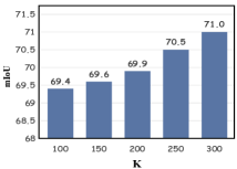
(a) Bank Size

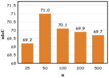
(b) Update Interval

Figure 4: Results of varying $K$ and $u$.

4.3 Analysis of Instance Feature Selection

The success of our DIDA largely lies in the introduction of instance-level discrimination, which can be ascribed to our meticulously designed dynamic memory bank mechanism and the proper selection of more informative source domain instances. Herein, we analyze how the bank size and different updating schemes can affect the effectiveness of DIDA.

Choice of Bank Size. As a general rule of thumb, the more instance features are stored, the model’s performance improves. We present results of varying different bank sizes $K$ in Figure 4(a), which validates this claim. Note that when $K$ surpasses 300, the consumption of storage increases to more than 23 GB, which pushes the GPU memory to its limit (24GB for a single RTX 3090 GPU). By limiting the bank size, our model is both friendly in memory occupation and efficient in adaptation. In the evaluation and the following ablation studies, our bank size $K$ is set to $300$.

Updating Strategies. This part includes experiments of update interval $u$, sampling strategy, and selecting strategy. Specifically, we sweep over [25, 50, 100, 200, 500] for update interval $u$. It’s obvious in Figure 4(b) that $u=50$ achieves the top result, while $u=25$ results in the worst. This is consistent with what MoCo [10] points out: a quickly changing feature bank leads to a dramatic reduction in performance. For updating features in the bank, we investigate no update (NU), random sampling (RS), inverted long-tail sampling (ILS), and class-balanced sampling (CBS). We also use AVG, KM, and BPS to represent average, K-means clustering, and boundary pixel selecting strategies. Please be aware that RS results in the long-tail distribution of classes and ILS leads to a “polar” condition of long-tail distribution (the original “head” becomes the new “tail”). Results are shown in Table 3.

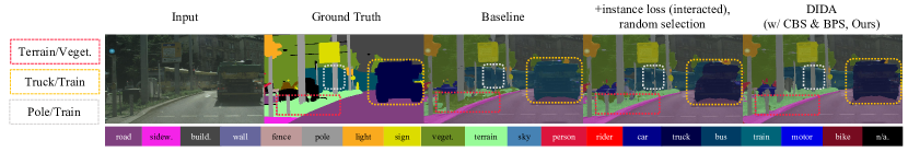
Figure 5: Visualized ablation of Sampling strategies.

Table 3: Ablation on sampling and selecting strategies

Sampling	mIoU	Selecting	mIoU
NU	68.6	RS	69.5
RS	69.5	AVG	69.7
ILS	69.0	KM	69.6
CBS	71.0	BPS	71.0

4.4 Ablation Studies

All ablation studies are conducted on the GTA5 $\rightarrow$ Cityscapes dataset. For more ablations, please refer to our supplementary material.

Smooth Parameters. Table 4 reveals the effect of gathering smooth parameters $\phi$ in Eq.(12). It indicates that the best proportion of semantic information locates at 0.9. We consider the extreme conditions as well: $\phi=1$ equals taking the original semantic pseudo-label for Eq.(5), while when $\phi=0$, the $\mathcal{L}_{tgt}$ oscillates and fails to converge.

Table 4: Results of different smooth parameters $\phi$

$\phi$	0	0.8	0.9	0.95	1.0
mIoU	fail	70.2	71.0	70.3	69.0

Pseudo-label regeneration Strategies. We also tried different combinations to find out the most suitable regeneration strategy to regenerate instance-level pseudo-label $\hat{q}$ and semantic-level pseudo-label $\hat{z}$. As observed from Table 5, applying smoothing to $\hat{z}$ and scaling to $\hat{q}$ obtains the top result. While there is very little difference from applying smoothing to the pseudo-labels from both levels (also achieves 70.9 mIoU), another smoothing parameter is then introduced in the process. Therefore, we prefer the scaling for $\hat{q}$ to keep a simpler framework

Table 5: Results of different interacting strategies $\phi$

	Smoothing	Scaling
Smoothing	70.9	71.0
Scaling	70.5	70.3

EMA Momentum. Table 6 shows mIoU performance with different ema momentum $\omega$ in Eq.(13). It performs reasonably from 0.9 to 0.999, demonstrating that a relatively slow-updating (i.e., larger momentum) instance bank is effective. Under the extreme condition $\omega=0$, the instance bank is purely updated with newly selected instance features, and the performance reduces dramatically. When $\omega=1$, it equals to “No Update” as conducted in the analysis of “Sampling Strategies”.

Table 6: Results of different ema momentum $\omega$

$\omega$	0	0.9	0.99	0.999	1.0
mIoU	68.9	70.3	70.6	71.0	69.4

Qualitative ablation on the Effectiveness of Sampling Strategies. Figure 5 presents the results of (1) baseline, (2) baseline with instance loss & interaction (pseudo-label regeneration) but the instances are randomly selected, and (3) DIDA, on segmenting an image containing “confusing” entities. We observe that the naive introduction of instance loss & interaction is helpful for common classes (e.g., “fence” and “vegetation” in red box), but lacks refinement on long-tailed/boundary pixels (the long-tailed classes of “truck” and “train” with some proportions of overlapping, in the yellow box), while CBS&BPS help to distinguish between the long-tailed and overlapping categories (a more explicit segmentation of “pole” from “train” and “truck” from “train”, in yellow & gray boxes). Please see more visualization results in our supplementary material.

Effect of each component. As displayed in Table 7, when considering additional instance-level similarity discrimination, we improve the baseline [14] by 0.9, revealing the effectiveness of our constructed feature bank. By applying updating strategies CBS and BPS, we explore the dominant factors of segmentation performance and witness a 0.6 gain. Finally, we introduce the pseudo-label regeneration (p.l.-reg.) to allow semantic-level and instance-level information to calibrate and balance each other, this mechanism leads to a further boost by 1.2. It’s worth noticing that when applying pseudo-label regeneration with randomly selected features to update the bank (i.e., w/o CBS&BPS), the performance gain is only 0.5. This is consistent with our previous assumption: a long-tailed distribution of instance features reduces the quality of regenerated pseudo-labels.

Table 7: Ablation of each proposed component.

ID	$\mathcal{L}_{ins}$	CBS	BPS	P.L.-Reg.	mIoU
baseline	$-$	$-$	$-$	$-$	68.3
I	$\checkmark$	$-$	$-$	$-$	69.2
II	$\checkmark$	$\checkmark$	$-$	$-$	69.6
III	$\checkmark$	$\checkmark$	$\checkmark$	$-$	69.8
IV	$\checkmark$	$-$	$-$	$\checkmark$	69.7
V	$\checkmark$	$\checkmark$	$\checkmark$	$\checkmark$	71.0

5 Discussion

Limitation & Future Directions. Although DIDA has achieved state-of-the-art performance on mainstream benchmarks using a single RTX 3090, it can be inferred that incorporating larger memory support could improve overall performance (refer to Sec. 4.3). To further improve performance, one may harness recent advancements in memory technologies, which could be based on Integer Linear Programming techniques [11] or DRAM management methods [27]. While a detailed investigation of this aspect falls outside the scope of our current work, we firmly believe that this avenue holds significant potential for future research. In addition, another future avenue resides in the generalizability of our Dual-level Interaction approach. Considering the strong similarity among the visual understanding tasks that heavily rely on extensive annotated data (e.g., object detection [8], instance segmentation [31], person re-identification [9]), our framework shows prominent applicability to other self-training scenarios in computer vision tasks.

6 Conclusion

This paper proposes a novel framework, DIDA, which for the first time introduces instance discrimination as an instance classifier to unsupervised domain adaptive semantic segmentation and interacts with semantic-level information for better noise adjustment. Unlike previous approaches, DIDA considers both semantic-level and instance-level information simultaneously. To tackle the issue of large storage consumption, we instantiate a dynamic instance feature bank and update it with carefully designed strategies. Additionally, our presented techniques of “scattering” and “gathering” facilitate interaction between the two levels and enable the regeneration of more robust pseudo-labels. Extensive experiments demonstrate DIDA’s superiority over previous methods. DIDA obtains significant IoU gains on confusing and long-tailed classes while achieving state-of-the-art overall performance. Discovering DIDA’s potential in other visual tasks is a promising direction, which will be our future work.

7 Acknowledgment

This research was supported in part by the National Key Research and Development Program of China under No.2021YFB3100700, the National Natural Science Foundation of China (NSFC) under Grants No. 62202340, Wuhan Knowledge Innovation Program under No. 2022010801020127.

References

- [1] Nikita Araslanov and Stefan Roth. Self-supervised augmentation consistency for adapting semantic segmentation. In Proceedings of the IEEE/CVF Conference on Computer Vision and Pattern Recognition, pages 15384–15394, 2021.
- [2] David Berthelot, Nicholas Carlini, Ian Goodfellow, Nicolas Papernot, Avital Oliver, and Colin A Raffel. Mixmatch: A holistic approach to semi-supervised learning. Advances in neural information processing systems, 32, 2019.
- [3] Yihong Cao, Hui Zhang, Xiao Lu, Yurong Chen, Zheng Xiao, and Yaonan Wang. Adaptive refining-aggregation-separation framework for unsupervised domain adaptation semantic segmentation. IEEE Transactions on Circuits and Systems for Video Technology, pages 1–1, 2023.
- [4] Yiting Cheng, Fangyun Wei, Jianmin Bao, Dong Chen, Fang Wen, and Wenqiang Zhang. Dual path learning for domain adaptation of semantic segmentation. In 2021 IEEE/CVF International Conference on Computer Vision (ICCV), pages 9062–9071, 2021.
- [5] Marius Cordts, Mohamed Omran, Sebastian Ramos, Timo Rehfeld, Markus Enzweiler, Rodrigo Benenson, Uwe Franke, Stefan Roth, and Bernt Schiele. The cityscapes dataset for semantic urban scene understanding. In Proceedings of the IEEE conference on computer vision and pattern recognition, pages 3213–3223, 2016.
- [6] Geoff French, Samuli Laine, Timo Aila, Michal Mackiewicz, and Graham Finlayson. Semi-supervised semantic segmentation needs strong, varied perturbations. arXiv preprint arXiv:1906.01916, 2019.
- [7] Geoffrey French, Michal Mackiewicz, and Mark Fisher. Self-ensembling for visual domain adaptation, 2018.
- [8] Guangxing Han, Yicheng He, Shiyuan Huang, Jiawei Ma, and Shih-Fu Chang. Query adaptive few-shot object detection with heterogeneous graph convolutional networks. In Proceedings of the IEEE/CVF International Conference on Computer Vision (ICCV), pages 3263–3272, October 2021.
- [9] Xin Hao, Sanyuan Zhao, Mang Ye, and Jianbing Shen. Cross-modality person re-identification via modality confusion and center aggregation. In Proceedings of the IEEE/CVF International Conference on Computer Vision (ICCV), pages 16403–16412, October 2021.
- [10] Kaiming He, Haoqi Fan, Yuxin Wu, Saining Xie, and Ross Girshick. Momentum contrast for unsupervised visual representation learning. In CVPR, pages 9729–9738, 2020.
- [11] Mark Hildebrand, Jawad Khan, Sanjeev Trika, Jason Lowe-Power, and Venkatesh Akella. Autotm: Automatic tensor movement in heterogeneous memory systems using integer linear programming. In Proceedings of the Twenty-Fifth International Conference on Architectural Support for Programming Languages and Operating Systems, pages 875–890, 2020.
- [12] Judy Hoffman, Eric Tzeng, Taesung Park, Jun-Yan Zhu, Phillip Isola, Kate Saenko, Alexei Efros, and Trevor Darrell. Cycada: Cycle-consistent adversarial domain adaptation. In International conference on machine learning, pages 1989–1998. Pmlr, 2018.
- [13] Judy Hoffman, Dequan Wang, Fisher Yu, and Trevor Darrell. Fcns in the wild: Pixel-level adversarial and constraint-based adaptation. arXiv preprint arXiv:1612.02649, 2016.
- [14] Lukas Hoyer, Dengxin Dai, and Luc Van Gool. Daformer: Improving network architectures and training strategies for domain-adaptive semantic segmentation. In Proceedings of the IEEE/CVF Conference on Computer Vision and Pattern Recognition, pages 9924–9935, 2022.
- [15] Jiaxing Huang, Dayan Guan, Aoran Xiao, Shijian Lu, and Ling Shao. Category contrast for unsupervised domain adaptation in visual tasks. In CVPR, pages 1203–1214, 2022.
- [16] Zhanghan Ke, Di Qiu, Kaican Li, Qiong Yan, and Rynson WH Lau. Guided collaborative training for pixel-wise semi-supervised learning. In Computer Vision–ECCV 2020: 16th European Conference, Glasgow, UK, August 23–28, 2020, Proceedings, Part XIII 16, pages 429–445. Springer, 2020.
- [17] Myeongjin Kim and Hyeran Byun. Learning texture invariant representation for domain adaptation of semantic segmentation, 2020.
- [18] Guangrui Li, Guoliang Kang, Wu Liu, Yunchao Wei, and Yi Yang. Content-consistent matching for domain adaptive semantic segmentation. In Andrea Vedaldi, Horst Bischof, Thomas Brox, and Jan-Michael Frahm, editors, Computer Vision – ECCV 2020, pages 440–456, Cham, 2020. Springer International Publishing.
- [19] Ruihuang Li, Shuai Li, Chenhang He, Yabin Zhang, Xu Jia, and Lei Zhang. Class-balanced pixel-level self-labeling for domain adaptive semantic segmentation. In CVPR, pages 11593–11603, 2022.
- [20] Yunsheng Li, Lu Yuan, and Nuno Vasconcelos. Bidirectional learning for domain adaptation of semantic segmentation. In 2019 IEEE/CVF Conference on Computer Vision and Pattern Recognition (CVPR), pages 6929–6938, 2019.
- [21] Weizhe Liu, David Ferstl, Samuel Schulter, Lukas Zebedin, Pascal Fua, and Christian Leistner. Domain adaptation for semantic segmentation via patch-wise contrastive learning, 2021.
- [22] Yahao Liu, Jinhong Deng, Xinchen Gao, Wen Li, and Lixin Duan. Bapa-net: Boundary adaptation and prototype alignment for cross-domain semantic segmentation. In Proceedings of the IEEE/CVF International Conference on Computer Vision (ICCV), pages 8801–8811, October 2021.
- [23] Yahao Liu, Jinhong Deng, Xinchen Gao, Wen Li, and Lixin Duan. Bapa-net: Boundary adaptation and prototype alignment for cross-domain semantic segmentation. In 2021 IEEE/CVF International Conference on Computer Vision (ICCV), pages 8781–8791, 2021.
- [24] J. MacQueen. Some methods for classification and analysis of multivariate observations. 1967.
- [25] Viktor Olsson, Wilhelm Tranheden, et al. Classmix: Segmentation-based data augmentation for semi-supervised learning, 2020.
- [26] Yassine Ouali, Céline Hudelot, and Myriam Tami. Semi-supervised semantic segmentation with cross-consistency training. In Proceedings of the IEEE/CVF Conference on Computer Vision and Pattern Recognition, pages 12674–12684, 2020.
- [27] Xuan Peng, Xuanhua Shi, Hulin Dai, Hai Jin, Weiliang Ma, Qian Xiong, Fan Yang, and Xuehai Qian. Capuchin: Tensor-based gpu memory management for deep learning. In Proceedings of the Twenty-Fifth International Conference on Architectural Support for Programming Languages and Operating Systems, pages 891–905, 2020.
- [28] Christian S. Perone, Pedro Ballester, Rodrigo C. Barros, and Julien Cohen-Adad. Unsupervised domain adaptation for medical imaging segmentation with self-ensembling, 2019.
- [29] Stephan R Richter, Vibhav Vineet, Stefan Roth, and Vladlen Koltun. Playing for data: Ground truth from computer games. In Computer Vision–ECCV 2016: 14th European Conference, Amsterdam, The Netherlands, October 11-14, 2016, Proceedings, Part II 14, pages 102–118. Springer, 2016.
- [30] German Ros, Laura Sellart, Joanna Materzynska, David Vazquez, and Antonio M Lopez. The synthia dataset: A large collection of synthetic images for semantic segmentation of urban scenes. In Proceedings of the IEEE conference on computer vision and pattern recognition, pages 3234–3243, 2016.
- [31] Josef Lorenz Rumberger, Xiaoyan Yu, Peter Hirsch, Melanie Dohmen, Vanessa Emanuela Guarino, Ashkan Mokarian, Lisa Mais, Jan Funke, and Dagmar Kainmüller. How shift equivariance impacts metric learning for instance segmentation. In Proceedings of the IEEE/CVF International Conference on Computer Vision (ICCV), pages 7128–7136, October 2021.
- [32] Kuniaki Saito, Donghyun Kim, Stan Sclaroff, and Kate Saenko. Universal domain adaptation through self supervision. Advances in neural information processing systems, 33:16282–16292, 2020.
- [33] Swami Sankaranarayanan, Yogesh Balaji, Arpit Jain, Ser Nam Lim, and Rama Chellappa. Learning from synthetic data: Addressing domain shift for semantic segmentation. In Proceedings of the IEEE conference on computer vision and pattern recognition, pages 3752–3761, 2018.
- [34] Inkyu Shin, Sanghyun Woo, Fei Pan, and InSo Kweon. Two-phase pseudo label densification for self-training based domain adaptation, 2020.
- [35] Kihyuk Sohn, David Berthelot, Nicholas Carlini, Zizhao Zhang, Han Zhang, Colin A Raffel, Ekin Dogus Cubuk, Alexey Kurakin, and Chun-Liang Li. Fixmatch: Simplifying semi-supervised learning with consistency and confidence. Advances in neural information processing systems, 33:596–608, 2020.
- [36] Antti Tarvainen and Harri Valpola. Mean teachers are better role models: Weight-averaged consistency targets improve semi-supervised deep learning results. Advances in neural information processing systems, 30, 2017.
- [37] Wilhelm Tranheden, Viktor Olsson, Juliano Pinto, and Lennart Svensson. Dacs: Domain adaptation via cross-domain mixed sampling. In Proceedings of the IEEE/CVF Winter Conference on Applications of Computer Vision, pages 1379–1389, 2021.
- [38] Thanh-Dat Truong, Chi Nhan Duong, Ngan Le, Son Lam Phung, Chase Rainwater, and Khoa Luu. Bimal: Bijective maximum likelihood approach to domain adaptation in semantic scene segmentation. In 2021 IEEE/CVF International Conference on Computer Vision (ICCV), pages 8528–8537, 2021.
- [39] Yi-Hsuan Tsai, Wei-Chih Hung, Samuel Schulter, Kihyuk Sohn, Ming-Hsuan Yang, and Manmohan Chandraker. Learning to adapt structured output space for semantic segmentation. In Proceedings of the IEEE conference on computer vision and pattern recognition, pages 7472–7481, 2018.
- [40] Midhun Vayyat, Jaswin Kasi, Anuraag Bhattacharya, Shuaib Ahmed, and Rahul Tallamraju. Cluda : Contrastive learning in unsupervised domain adaptation for semantic segmentation, 2022.
- [41] Tuan-Hung Vu, Himalaya Jain, Maxime Bucher, Matthieu Cord, and Patrick Pérez. Advent: Adversarial entropy minimization for domain adaptation in semantic segmentation. In Proceedings of the IEEE/CVF Conference on Computer Vision and Pattern Recognition, pages 2517–2526, 2019.
- [42] Yuxi Wang, Junran Peng, et al. Uncertainty-aware pseudo label refinery for domain adaptive semantic segmentation. In ICCV, pages 9072–9081, 2021.
- [43] Yuxi Wang, Junran Peng, and Zhaoxiang Zhang. Uncertainty-aware pseudo label refinery for domain adaptive semantic segmentation. In 2021 IEEE/CVF International Conference on Computer Vision (ICCV), pages 9072–9081, 2021.
- [44] Zhonghao Wang, Mo Yu, Yunchao Wei, Rogerio Feris, Jinjun Xiong, Wen mei Hwu, Thomas S. Huang, and Humphrey Shi. Differential treatment for stuff and things: A simple unsupervised domain adaptation method for semantic segmentation, 2020.
- [45] Zhirong Wu, Yuanjun Xiong, Stella X Yu, and Dahua Lin. Unsupervised feature learning via non-parametric instance-level discrimination. preprint arXiv:1805.01978, 2018.
- [46] Enze Xie, Wenhai Wang, Zhiding Yu, Anima Anandkumar, Jose M Alvarez, and Ping Luo. Segformer: Simple and efficient design for semantic segmentation with transformers. Advances in Neural Information Processing Systems, 34:12077–12090, 2021.
- [47] Sangdoo Yun, Dongyoon Han, Seong Joon Oh, Sanghyuk Chun, Junsuk Choe, and Youngjoon Yoo. Cutmix: Regularization strategy to train strong classifiers with localizable features. In Proceedings of the IEEE/CVF international conference on computer vision, pages 6023–6032, 2019.
- [48] Pan Zhang, Bo Zhang, Ting Zhang, Dong Chen, Yong Wang, and Fang Wen. Prototypical pseudo label denoising and target structure learning for domain adaptive semantic segmentation. In Proceedings of the IEEE/CVF conference on computer vision and pattern recognition, pages 12414–12424, 2021.
- [49] Yang Zou, Zhiding Yu, BVK Kumar, and Jinsong Wang. Unsupervised domain adaptation for semantic segmentation via class-balanced self-training. In Proceedings of the European conference on computer vision (ECCV), pages 289–305, 2018.
- [50] Yang Zou, Zhiding Yu, B. V. K. Vijaya Kumar, and Jinsong Wang. Domain adaptation for semantic segmentation via class-balanced self-training, 2018.