Kecor: Kernel Coding Rate Maximization for Active 3D Object Detection

Abstract

Achieving a reliable LiDAR-based object detector in autonomous driving is paramount, but its success hinges on obtaining large amounts of precise 3D annotations. Active learning (AL) seeks to mitigate the annotation burden through algorithms that use fewer labels and can attain performance comparable to fully supervised learning. Although AL has shown promise, current approaches prioritize the selection of unlabeled point clouds with high uncertainty and/or diversity, leading to the selection of more instances for labeling and reduced computational efficiency. In this paper, we resort to a novel kernel coding rate maximization (Kecor) strategy which aims to identify the most informative point clouds to acquire labels through the lens of information theory. Greedy search is applied to seek desired point clouds that can maximize the minimal number of bits required to encode the latent features. To determine the uniqueness and informativeness of the selected samples from the model perspective, we construct a proxy network of the 3D detector head and compute the outer product of Jacobians from all proxy layers to form the empirical neural tangent kernel (NTK) matrix. To accommodate both one-stage (i.e., Second) and two-stage detectors (i.e., Pv-rcnn), we further incorporate the classification entropy maximization and well trade-off between detection performance and the total number of bounding boxes selected for annotation. Extensive experiments conducted on two 3D benchmarks and a 2D detection dataset evidence the superiority and versatility of the proposed approach. Our results show that approximately 44% box-level annotation costs and 26% computational time are reduced compared to the state-of-the-art AL method, without compromising detection performance.

1 Introduction

Being a crucial component in the realm of scene understanding, LiDAR-based 3D object detection [58, 63, 34, 59] identifies and accurately localizes objects in a 3D scene with the oriented bounding boxes and semantic labels. This technology has facilitated a wide range of applications in environmental perceptions, including robotics, autonomous driving, and augmented reality. With the recent advancements in 3D detection models [53, 14, 25], highly accurate recognition of objects can be achieved through point cloud projection [64], point feature extraction [59, 67, 66, 34, 57] or voxelization [58, 13, 63]. However, achieving such performance often comes at the expense of requiring a large volume of labeled point cloud data, which can be costly and time-consuming.

To mitigate the labeling costs and optimize the value of annotations, active learning (AL) [49, 37] has emerged as a promising solution. Active learning involves iteratively selecting the most beneficial samples for label acquisition from a large pool of unlabeled data until the labeling budget is exhausted. This selection process is guided by the selection criteria based on sample uncertainty [36, 29, 50, 48] and/or diversity [55, 16, 22, 65]. Both measures are used to assess the informativeness of the unlabeled samples. Aleatoric uncertainty-driven approaches search for samples that the model is least confident of by using metrics like maximum entropy [62] or estimated model changes [68, 44]. On the other hand, epistemic uncertainty based methods attempt to find the most representative samples to avoid sample redundancy by using greedy coreset algorithms [55] or clustering based approaches [5].

While active learning has proven to be effective in reducing labeling costs for recognition tasks, its application in LiDAR-based object detection has been limited [18, 54, 30]. This is largely due to its high computational costs and involvement of both detection and regression tasks, which pose significant challenges to the design of the selection criteria. A very recent work Crb [41] manually designed three heuristics that allow the acquisition of labels by hierarchically filtering out concise, representative, and geometrically balanced unlabelled point clouds. While effective, it remains unclear how to characterize the sample informativeness for both classification and regression tasks with one unified measurement.

In this paper, we propose a novel AL strategy called kernel coding rate maximization (Kecor) for efficient and effective active 3D detection. To endow the model with the ability to reason about the trade-off between information and performance autonomously, we resort to the coding rate theory and modify the formula from feature selection to sample selection, by replacing the covariance estimate with the empirical neural tangent kernel (NTK). The proposed Kecor strategy allows us to pick the most informative point clouds from the unlabeled pool such that their latent features require the maximal coding length for encoding. To characterize the non-linear relationships between the latent features and the corresponding box predictions spending the least computational costs, we train a proxy network of the 3D detector head with labeled samples and extract the outer product of Jacobians from all proxy layers to form the NTK matrix of all unlabeled samples. Empirical studies evidence that the NTK kernel not only captures non-linearity but takes the aleatoric and epistemic uncertainties into joint consideration, assisting detectors to recognize challenging objects that are of sparse structure. To accommodate both one-stage (i.e., Second) and two-stage detectors (i.e., Pv-rcnn), we further incorporate the classification entropy maximization into the selection criteria. Our contributions are summarized as below:

1. We propose a novel information-theoretic based criterion Kecor for cost-effective 3D box annotations that allows for the greedy search of informative point clouds by maximizing the kernel coding rate.

2. Our framework is flexible to accommodate different choices of kernels and 3D detector architectures. Empirical NTK kernel used in Kecor demonstrates a strong capacity to unify both aleatoric and epistemic uncertainties from the model perspective, which helps detectors learn a variety of challenging objects.

3. Extensive experiments have been conducted on both 3D benchmarks (i.e., KITTI and Waymo Open) and 2D object detection dataset (i.e., PASCAL VOC07), verifying the effectiveness and versatility of the proposed approach. Experimental results show that the proposed approach achieves a 44.4% reduction of annotations and up to 26.4% less running time compared to the state-of-the-art active 3D detection methods.

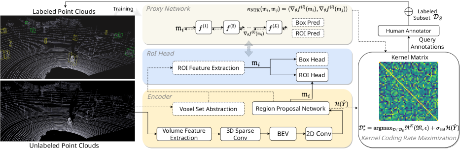
Figure 1: An illustration of the workflow of the proposed kernel coding rate maximization for active 3D detection. Dotted boxes indicate the unique components in two-stage 3D detectors (e.g., Pv-rcnn), while solid boxes indicate the shared components in both one-stage (e.g., Second) and two-stage detectors.

2 Related Work

2.1 Active Learning (AL)

Active learning has been widely applied to image classification and regression tasks, where the samples that lead to unconfident predictions (i.e., aleatoric uncertainty) [61, 61, 36, 29, 50, 48, 15, 32, 7, 56, 51, 19, 68] or not resemble the training set (i.e., epistemic uncertainty) [55, 16, 22, 65, 45, 24, 2, 44] will be selected and acquired for annotations. Hybrid methods [31, 11, 5, 43, 40, 33, 26] unify both types of uncertainty to form an acquisition criterion. Examples include Badge [5] and Bait [4], which select a batch of samples that probably induce large and diverse changes to the model based on the gradients and Fisher information.

AL for Detection. Research on active learning for object detection [52, 71, 30, 23, 9, 69] has not bee as widespread as that for image classification, due in part to the challenges in quantifying aleatoric and epistemic uncertainties in bounding box regression. Kao et al. [30] proposed two metrics to quantitatively evaluate the localization uncertainty, where the samples containing inconsistent box predictions will be selected. Choi et al. [9] predicted the parameters of the Gaussian mixture model and computes epistemic uncertainty as the variance of Gaussian models. Agarwal et al. [1] proposed a contextual diversity measurement for selecting unlabeled images containing objects in diverse backgrounds. Park et al. [47] determined epistemic uncertainty by using evidential deep learning along with hierarchical uncertainty aggregation to effectively capture the context within an image. Wu et al. [62] introduced a hybrid approach, which utilizes an entropy-based non-maximum suppression to estimate uncertainty and a diverse prototype strategy to ensure diversity. Nevertheless, the application of active learning to 3D point cloud detection is still under-explored due to the high computational costs, which makes AL strategies such as adding additional detection heads [9] or augmentations [69] impractical. Previous solutions [18, 54, 6, 20] rely on generic metrics such as Shannon entropy [61], localization tightness [30] for measuring aleatoric uncertainty. Only a recent work Crb [41] exploited both uncertainties jointly by greedily searching point clouds that have concise labels, representative features and geometric balance. Different from Crb that hierarchically filters samples with three criteria, in this work, we derive an informatic-theoretic criterion, namely kernel coding rate, that enables informativeness measurement in a single step and saves computational costs by 26%.

2.2 Coding Rate

Entropy, rate distortion [12, 8] and coding rate [42] are commonly used measurements to quantify the uncertainty and compactness of a random variable $\mathbf{Z}$. They can be interpreted as the “goodness” of the latent representations in deep neural networks with respect to generalizability [39], transferability [27] and robustness. Entropy $\mathcal{H}(\mathbf{Z})$ calculates the expected value of the negative logarithm of the probability, while it is not well-defined for a continuous random variable with degenerate distributions [70]. To address this, rate distortion $\mathfrak{R}(\mathbf{Z},\epsilon)$ is proposed in the context of lossy data compression, which quantifies the minimum average number of binary bits required to represent $\mathbf{Z}$. Given the calculation difficulty of distortion rate, coding rate $\mathfrak{R}(\mathbf{Z})$ emerges as a more feasible solution for quantifying random variables from a complex distribution (refer to Section 3.2). Unlike prior works mentioned above, our work explores a new kernel coding rate for sample selection in active learning rather than feature selection.

2.3 Neural Tangent Kernel

Neural tangent kernel (NTK) [28, 35, 46, 3] is a kernel that reveals the connections between infinitely wide neural networks trained by gradient descent and kernel methods. NTK enables the study of neural networks using theoretical tools from the perspective of kernel methods. There have been several studies that have explored the properties of NTK: Jacot et al. [28] proposed the concept of NTK and showed that it could be used to explain the generalization of neural networks. Lee et al. [35] expanded on this work and demonstrated that the dynamics of training wide but finite-width NNs with gradient descent can be approximated by a linear model obtained from the first-order Taylor expansion of that network around its initialization. In this paper, rather than exploring the interpretability of infinite-width neural networks, we explore empirical (i.e., finite-width) neural tangent kernels to improve linear kernels and non-linear RBF kernels. The NTK is used to characterize the sample similarity based on 3D detector head behaviors, which naturally takes aleatoric and epistemic uncertainties into consideration.

3 Preliminaries

In this section, we present the mathematical formulation of the problem of active learning for 3D object detection, along with the establishment of the necessary notations.

3.1 Problem Formulation

3D Object Detection. The typical approach for detecting objects in an orderless point cloud $\mathcal{P}_{i}$ involves training a 3D object detector to identify and locate the objects of interest, consisting of a set of 3D bounding boxes and their labels $\mathfrak{B}_{i}=\{b_{k},y_{k}\}_{k\in[N_{i}]}$, with $N_{i}$ indicating the number of bounding boxes in the $i$-th point cloud. Each point in $\mathcal{P}_{i}=\{(x,y,z,r)\}$ is represented by xyz spatial coordinates and additional features such as reflectance $r$. The box annotations $b_{k}\in\mathbb{R}^{7}$ include the relative center xyz spatial coordinates to the object ground planes, the box size, the heading angle, and the box label $y_{k}\in\mathbb{R}^{C}$, where $C$ indicates the number of classes. As illustrated in Figure 1, modern 3D detectors extract latent features $\mathfrak{m}_{i}=\bm{g}(\mathcal{P}_{i};\bm{\theta}_{g})\in\mathbb{R}^{d}$ through projection [64], PointNet encoding [59, 67, 66, 34, 57] or voxelization [58, 13, 63], where dimension $d=W\times H\times F$ is the product of width $W$, length $H$, and channels $F$ of the feature map. The detection head $\bm{h}(\cdot;\bm{\theta}_{h})$ uses $\mathfrak{m}_{i}$ as inputs and generates detection outcomes $\mathfrak{\hat{B}}_{i}=\{\hat{b}_{k},\hat{y}_{k}\}$:

$$\mathcal{P}_{i}\xmapsto{\bm{g}(\cdot;\bm{\theta}_{g})}\mathfrak{m}_{i}\xmapsto{\bm{h}(\cdot;\bm{\theta}_{h})}\mathcal{\mathfrak{\hat{B}}}_{i}.$$ (1)

Active Learning Setup. In an active learning setup, a small set of labeled point clouds $\mathcal{D}_{L}=\{\mathcal{P}_{i},\mathfrak{B}_{i}\}_{i\in L}$ and a large pool of raw point clouds $\mathcal{D}_{U}=\{\mathcal{P}_{j}\}_{j\in U}$ are given at training time, where $L$ and $U$ are the index sets corresponding to $\mathcal{D}_{L}$ and $\mathcal{D}_{U}$, respectively, and the cardinality of each set satisfy that $|L|\ll|U|$. During each active learning round $r\in\{1,\ldots,R\}$, a subset of point clouds $\mathcal{D}_{r}^{*}$ is selected from $\mathcal{D}_{U}$ based on a defined active learning policy. The labels of 3D bounding boxes for the chosen point clouds are queried from an oracle $\bm{\Omega}:\mathcal{P}\mapsto\mathfrak{B}$ to create a labeled set $\mathcal{D}_{S}=\{\mathcal{P}_{j},\mathfrak{B}_{j}\}_{\mathcal{P}_{j}\in\mathcal{D}_{r}^{*}}$. The 3D detection model is pre-trained with $\mathcal{D}_{L}$ for active selection and then retrained with $\mathcal{D}_{S}\cup\mathcal{D}_{L}$. The process is repeated until the selected samples reach the final budget $B$, i.e., $\sum_{r=1}^{R}|\mathcal{D}_{r}^{*}|=B$.

3.2 Coding Rate

As explained in Section 2.2, information theory [12] defines the coding rate $\mathfrak{R}(\cdot,\epsilon)$ [42] as a measure of lossy data compression, quantifying the achievability of maximum compression while adhering to a desired error upper bound. It is commonly used as an empirical estimation of rate distortion [12, 8] indicating the minimal number of binary bits required to represent random variable $\mathbf{Z}$ with the expected decoding error below $\epsilon$. Given a finite set of $n$ samples $\mathbf{Z}=[\mathbf{z}_{1},\mathbf{z}_{2},...,\mathbf{z}_{n}]\in\mathbb{R}^{d\times n}$, the coding rate [42] with respect to $\mathbf{Z}$ and a distortion $\epsilon$ is given by:

$$\vspace{-1ex}\mathfrak{R}(\mathbf{Z},\epsilon)=\frac{1}{2}\log\text{det}(\mathbf{I}+\frac{d}{\epsilon^{2}n}\hat{\Sigma}),$$ (2)

where $\mathbf{I}$ is the $d$-dimensional identify matrix and $\hat{\Sigma}=\mathbf{Z}\mathbf{Z}^{\mkern-1.5mu\mathsf{T}}\in\mathbb{R}^{d\times d}$ is an estimate of covariance. Theoretical justifications have been provided in [42] that the coding vectors in $\mathbf{Z}$ can be explained by packing $\epsilon$-balls into the space spanned by $\mathbf{Z}$ (sphere packing [12]) or by computing the number of bits needed to quantize the SVD of $\mathbf{Z}$ subject to the precision. As coding rate produces a good estimate of the compactness of latent features, a few attempts [10, 39] have been made in the areas of multi-view learning and contrastive learning, which select informative features from $d$ dimensions by maximizing the coding rate.

4 Proposed Approach

4.1 Kernel Coding Rate Maximization

The core task in pool-based active learning is to select the most informative samples from the unlabeled pool $\mathcal{D}_{U}$, which motivates us to replace the covariance estimate of features with the kernel matrix of samples in the coding rate formula (see Equation (2)). To each point cloud subset $\mathcal{D}=\{\mathcal{P}_{i}\}_{i=1}^{n}\subset\mathcal{D}_{U}$ of size $n$, we refer to this new coding length $\mathfrak{R}^{K}(\mathfrak{M},\epsilon)$ as the kernel coding rate, which represents the minimal number of bits to encode features $\mathfrak{M}$:

$$\mathfrak{M}=\bm{g}(\mathcal{D},\bm{\theta}_{g})=[\mathfrak{m}_{1},\mathfrak{m}_{2},...,\mathfrak{m}_{n}]\in\mathbb{R}^{d\times n}.\vspace{-1ex}$$

The latent features extracted from $\bm{g}(\cdot;\bm{\theta}_{g})$ can help find the most informative samples irrespective of the downstream tasks of classification and/or regression. We mathematically define the kernel coding rate $\mathfrak{R}^{K}(\mathfrak{M},\epsilon)$ as:

$$\mathfrak{R}^{K}(\mathfrak{M},\epsilon):=\frac{1}{2}\log\text{det}(\mathbf{I}+\frac{n}{\epsilon^{2}d}\mathbf{K}_{\mathfrak{M},\mathfrak{M}}),$$ (3)

with the kernel matrix $\mathbf{K}_{\mathfrak{M},\mathfrak{M}}=[K(\mathfrak{m}_{i},\mathfrak{m}_{j})]\in\mathbb{R}^{n\times n}$. In each round $r\in\{1,\ldots,R\}$, we use greedy search to find an optimal subset $\mathcal{D}_{r}^{*}$ with size $n$ from the unlabeled pool $\mathcal{D}_{U}$ by maximizing the kernel coding rate:

$$\vspace{-1ex}\mathcal{D}_{r}^{*}=\operatorname*{arg\,max}_{\mathcal{D}\subset\mathcal{D}_{U}\text{with}|\mathcal{D}|=n}\mathfrak{R}^{K}(\mathfrak{M},\epsilon),$$ (4)

where $\mathfrak{M}=\bm{g}(\mathcal{D};\bm{\theta}_{g})$. Notably, in the above equation, we consider positive semi-definite (PSD) kernel $K:\mathfrak{m}\times\mathfrak{m}\rightarrow\mathbb{R}$, which characterizes the similarity between each pair of embeddings of point clouds, and hence, helps with avoiding redundancy. The most basic type of PSD kernel to consider is linear kernel, which is defined by the dot product between two features:

$$K_{\operatorname{Linear}}(\mathfrak{m}_{i},\mathfrak{m}_{j})=\langle\mathfrak{m}_{i},\mathfrak{m}_{j}\rangle=\mathfrak{m}_{i}^{\mkern-1.5mu\mathsf{T}}\mathfrak{m}_{j}.\vspace{-1ex}$$ (5)

This kernel can be computed very quickly yet it has limitations when dealing with high-dimensional input variables, such as in our case where $d=W\times L\times F$. The linear kernel may capture the noise and fluctuations in the data instead of the underlying pattern, making it less generalizable to the unseen data. Therefore, while the linear kernel can be a useful starting point, it may be necessary to consider other PSD kernels that are better suited to the specific characteristics of the point cloud data at hand. More discussion on non-linear kernels (e.g., Laplace RBF kernel) is provided in the supplementary material. In the following subsection, we explain a more appropriate PSD kernel $K$ to be used in Kecor, where we can jointly consider aleatoric and epistemic uncertainties from the model perspective.

4.1.1 Empirical Neural Tangent Kernel $K_{\operatorname{NTK}}$

Compared with linear kernel, empirical neural tangent kernel (NTK) [28, 46] defined as the outer product of the neural network Jacobians, has been shown to lead to improved generalization performance in deep learning models. The yielded NTK matrix quantifies how changes in the inputs affect the outputs and captures the relationships between the inputs and outputs in a compact and interpretable way.

To efficiently compute the NTK kernel matrix, we first consider a $(L+1)$-layer fully connected neural network $\bm{f}(\cdot;\bm{\theta}):\mathfrak{m}\mapsto\hat{\mathfrak{B}}$ as a proxy network for the detection head $\bm{h}(\cdot;\bm{\theta}_{h})$, as shown in Figure 1. The $l$-th layer in the proxy network $\bm{f}$ has $d_{l}$ neurons, where $l$ ranges from $0$ to $L$. In the forward pass computation, the output from the $l$-th layer is defined as,

$$\bm{f}^{(l)}(\mathfrak{m}_{i};\bm{\theta}^{(l)})=\sigma(\frac{1}{\sqrt{d_{l}}}\bm{W}^{(l)}\bm{f}^{(l-1)}(\mathfrak{m}_{i})+\beta\bm{b}^{(l)}),$$ (6)

where $\beta\geq 0$ is a constant controlling the effect of bias and $\bm{f}^{0}(\mathfrak{m}_{i})=\mathfrak{m}_{i}$. $\sigma(\cdot)$ stands for a pointwise nonlinear function. Note that the weight matrix $\bm{W}^{(l)}\in\mathbb{R}^{d_{l}\times d_{l-1}}$ is rescaled by $1/\sqrt{d_{l}}$ to avoid divergence, which refers to NTK parameterization [28]. For notation simplicity, we denote $\bm{f}^{(l)}(\mathfrak{m}_{i};\bm{\theta}^{(l)})$ as $\bm{f}^{(l)}_{i}$. We omit the bias term and rewrite Equation (6) as

$$\bm{f}^{(l)}_{i}=\bm{\tilde{W}}^{(l)}\mathfrak{\tilde{m}}_{i}^{(l-1)},$$ (7)

where $\tilde{\bm{W}}^{(l)}=[\bm{W}^{(l)},\bm{b}^{(l)}]\in\mathbb{R}^{d_{l}\times(d_{l-1})+1}$, $\mathfrak{\tilde{m}}_{i}^{(l-1)}=[\frac{\sigma}{\sqrt{d_{l}}}\bm{f}_{i}^{(l-1)};\sigma\beta]\in\mathbb{R}^{d_{l-1}+1}$. We denote all parameters in the proxy network as $\bm{\theta}=[\tilde{\bm{W}}^{(1)},\ldots,\tilde{\bm{W}}^{(L)}]$. To endow the proxy network $\bm{f}$ with the capability to mimic the behavior of the detector head, we train the proxy $\bm{f}$ with the labeled data $\mathcal{D}_{L}$ by using an empirical regression loss function $\mathcal{L}:\mathbb{R}^{d_{L}}\rightarrow\mathbb{R}_{+}$ e.g., mean squared error (MSE) to supervise the 3D box and ROI predictions. It is found that training neural networks using the MSE loss involves solving a linear regression problem with the kernel trick [28], where the kernel $K_{\operatorname{NTK}}$ is defined as the derivative of the output of a neural network with respect to its inputs at the $l$-th layer, evaluated at the initial conditions:

$$K_{\operatorname{NTK}}(\mathfrak{m}_{i},\mathfrak{m}_{j})=\langle\nabla_{\bm{\theta}}\bm{f}^{(l)}(\mathfrak{\bm{m}}_{i}),\nabla_{\bm{\theta}}\bm{f}^{(l)}(\mathfrak{\bm{m}}_{j})\rangle.$$ (8)

By incorporating Equation (7) and the chain rule, we obtain the factorization of derivates as the ultimate form of empirical NTK kernel:

$$\begin{split}K_{\operatorname{NTK}}(\mathfrak{m}_{i},\mathfrak{m}_{j})&=\sum_{l=1}^{L}\langle\frac{\mathrm{d}\bm{f}_{i}^{(L)}}{\mathrm{d}\bm{f}_{i}^{(l)}}\left(\tilde{\mathfrak{m}}_{i}^{(l-1)}\right)^{\mkern-1.5mu\mathsf{T}},\frac{\mathrm{d}\bm{f}_{j}^{(L)}}{\mathrm{d}\bm{f}_{j}^{(l)}}\left(\tilde{\mathfrak{m}}_{j}^{(l-1)}\right)^{\mkern-1.5mu\mathsf{T}}\rangle_{F}\\ &=\sum_{l=1}^{L}\left\langle\tilde{\mathfrak{m}}_{i}^{(l-1)},\tilde{\mathfrak{m}}_{j}^{(l-1)}\right\rangle\cdot\left\langle\frac{\mathrm{d}\bm{f}_{i}^{(L)}}{\mathrm{d}\bm{f}_{i}^{(l)}},\frac{\mathrm{d}\bm{f}_{j}^{(L)}}{\mathrm{d}\bm{f}_{j}^{(l)}}\right\rangle,\end{split}$$

where $\langle\cdot,\cdot\rangle_{F}$ indicates the Frobenius inner product. The above equation demonstrates that the NTK kernel is constructed by taking into account the gradient contributions from multiple layers, which naturally captures the epistemic uncertainty in the detector’s behavior.

4.1.2 Last-layer Gradient Kernel $K_{\operatorname{Last}}$

To verify the validity of aggregating gradients from multiple layers, we derive a simplified variant of the NTK kernel $K_{\operatorname{NTK}}$, which only considers the gradients w.r.t the parameters from the last layer of the proxy network:

$$K_{\operatorname{Last}}(\mathfrak{m}_{i},\mathfrak{m}_{j})=\langle\nabla_{\tilde{\bm{W}}^{(L)}}\bm{f}^{(l)}(\mathfrak{\bm{m}}_{i}),\nabla_{\tilde{\bm{W}}^{(L)}}\bm{f}^{(l)}(\mathfrak{\bm{m}}_{j})\rangle.$$ (9)

We have conducted extensive experiments to compare the impact of different kernels selected in the kernel coding rate maximization criteria as shown in Section 5.4.1. Empirical results suggest that the one-stage detectors generally favor $K_{\operatorname{Last}}$ while two-stage detectors tend to perform better with $K_{\operatorname{NTK}}$ on 3D detection recognition tasks.

4.2 Acquisition Function

As described in Equation (4), our approach selects the most informative point clouds based on the extracted features $\mathfrak{m}$ and gradient maps and thereby facilitate downstream predictions in the detector head. However, for two-stage detectors like Pv-rcnn, the classification prediction is made in the region proposal network (refer to dotted boxes and lines in Figure 1) before feeding features into the detector head. Therefore, the features $\mathfrak{m}$ alone cannot determine the informativeness for the box classification task. To make the proposed Kecor strategy applicable to both one-stage and two-stage detectors, we introduce the modified acquisition function by including an entropy regularization term as below:

$$\mathcal{D}_{r}^{*}=\operatorname*{arg\,max}_{\mathcal{D}\subset\mathcal{D}_{U}\text{with}|\mathcal{D}|=n}\mathfrak{R}^{K}(\mathfrak{M},\epsilon)+\sigma_{\operatorname{ent}}\mathcal{H}(\hat{Y}),\vspace{-0.5ex}$$ (10)

where $\mathcal{H}(\cdot)$ represents the mean entropy of all classification logits generated from the classifier. The effect of the hyperparameter $\sigma_{\operatorname{ent}}$ is studied in Section 5.4.2. The overall algorithm is summarized in the supplementary material.

5 Experiments

5.1 Experimental Setup

3D Point Cloud Detection Datasets. KITTI [21] is one of the most representative datasets for point cloud based object detection. The dataset consists of 3,712 training samples (i.e., point clouds) and 3,769 val samples. The dataset includes a total of 80,256 labeled objects with three commonly used classes for autonomous driving: cars, pedestrians, and cyclists. The Waymo Open dataset [60] is a challenging testbed for autonomous driving, containing 158,361 training samples and 40,077 testing samples. The sampling intervals for KITTI and Waymo are set to 1 and 10, respectively. To fairly evaluate baselines and the proposed method on KITTI dataset [21], we follow the work of [58]: we utilize Average Precision (AP) for 3D and Bird Eye View (BEV) detection, and the task difficulty is categorized to Easy, Moderate, and Hard, with a rotated IoU threshold of $0.7$ for cars and $0.5$ for pedestrian and cyclists. The results evaluated on the validation split are calculated with $40$ recall positions. To evaluate on Waymo dataset [60], we adopt the officially published evaluation tool for performance comparisons, which utilizes AP and the Average Precision Weighted by Heading (APH). The respective IoU thresholds for vehicles, pedestrians, and cyclists are set to 0.7, 0.5, and 0.5. Regarding detection difficulty, the Waymo test set is further divided into two levels. Level 1 (and Level 2) indicates there are more than five inside points (at least one point) in the ground-truth objects.

2D Image Detection Dataset. On the PASCAL VOC 2007 dataset [17], we use 4,000 images in the trainval set for training and 1,000 images in the test set for testing. For active selection, we set 500 labeled images as random initialization. Then $n=$500 images are labeled at each cycle until reaching 2,000. The trained SSD [38] detectors are evaluated with mean Average Precision (mAP) at IoU = 0.5 on VOC07. Unspecified training details are the same as in [9].

Table 1: Performance comparisons on the 3D AP (%) scores with generic AL and applied AL for detection on KITTI val set with 1% queried bounding boxes. Pv-rcnn is used as the backbone architecture for all approaches.

		Car			Pedestrian			Cyclist			Average
	Method	Easy	Mod.	Hard	Easy	Mod.	Hard	Easy	Mod.	Hard	Easy	Mod.	Hard
Generic	Coreset[55]	87.77	77.73	72.95	47.27	41.97	38.19	81.73	59.72	55.64	72.26	59.81	55.59
	Badge[5]	89.96	75.78	70.54	51.94	46.24	40.98	84.11	62.29	58.12	75.34	61.44	56.55
	Llal[68]	89.95	78.65	75.32	56.34	49.87	45.97	75.55	60.35	55.36	73.94	62.95	58.88
AL Detection	Mc-reg [41]	88.85	76.21	73.47	35.82	31.81	29.79	73.98	55.23	51.85	66.21	54.41	51.70
	Mc-mi [18]	86.28	75.58	71.56	41.05	37.50	33.83	86.26	60.22	56.04	71.19	57.77	53.81
	Consensus[54]	90.14	78.01	74.28	56.43	49.50	44.80	78.46	55.77	53.73	75.01	61.09	57.60
	Lt/c[30]	88.73	78.12	73.87	55.17	48.37	43.63	83.72	63.21	59.16	75.88	63.23	58.89
	Crb[41]	90.98	79.02	74.04	64.17	54.80	50.82	86.96	67.45	63.56	80.70	67.81	62.81
	Kecor	91.71	79.56	74.05	65.37	57.33	51.56	87.80	69.13	64.65	81.63	68.67	63.42

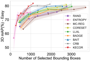
(a)

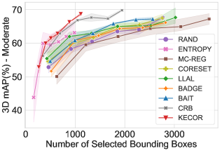
(b)

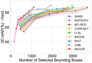
(c)

Figure 2: 3D mAP (%) of Kecor and AL baselines on the KITTI val split with Pv-rcnn.

Implementation Details. To ensure the reproducibility of the baselines and the proposed approach, we implement Kecor based on the public Active-3D-Det [41] toolbox that can accommodate most of the public LiDAR detection benchmark datasets. The hyperparameter $\sigma_{\operatorname{ent}}$ is fixed to $0.1$ and $0.5$ on the KITTI and Waymo Open datasets, respectively. The hyperparameter $\beta$ is set to 0.1, which is consistent with [42]. For the proxy network, we build two-layer fully connected networks, with the latent dimensions $d_{1}$ and $d_{2}$ fixed to 256. The source code and other implementation details of active learning protocols can be found in the supplementary material for reference.

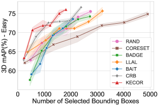
(a)

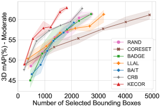
(b)

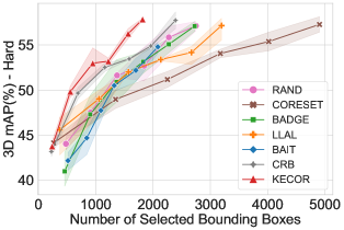
(c)

Figure 3: 3D mAP (%) of Kecor and AL baselines on the KITTI val split with Second.

Table 2: 3D mAP and BEV scores (%) on the KITTI val split with one-stage 3D detector Second.

		3D Detection mAP			BEV Detection mAP
	Venue	Easy	Moderate	Hard	Easy	Moderate	Hard
Rand		$69.33_{\pm 0.62}$	$55.48_{\pm 0.43}$	$51.53_{\pm 0.33}$	$75.66_{\pm 1.10}$	$63.77_{\pm 0.86}$	$59.71_{\pm 0.95}$
Coreset[55]	ICLR’18	$66.86_{\pm 2.27}$	$53.22_{\pm 1.65}$	$48.97_{\pm 1.42}$	$73.08_{\pm 1.80}$	$61.03_{\pm 1.98}$	$56.95_{\pm 1.53}$
Llal[68]	CVPR’19	$69.19_{\pm 3.43}$	$55.38_{\pm 3.63}$	$50.85_{\pm 3.24}$	$76.52_{\pm 2.24}$	$63.25_{\pm 3.11}$	$59.07_{\pm 2.80}$
Badge[5]	ICLR’20	$69.92_{\pm 2.90}$	$55.60_{\pm 2.72}$	$51.23_{\pm 2.58}$	$76.07_{\pm 2.70}$	$63.39_{\pm 2.52}$	$59.47_{\pm 2.49}$
Bait [4]	NeurIPS’21	$69.45_{\pm 3.53}$	$55.61_{\pm 2.94}$	$51.25_{\pm 2.42}$	$76.04_{\pm 1.75}$	$63.49_{\pm 2.14}$	$53.40_{\pm 2.00}$
Crb[41]	ICLR’23	$72.33_{\pm 0.35}$	$58.06_{\pm 0.30}$	$53.09_{\pm 0.31}$	$78.84_{\pm 0.27}$	$65.82_{\pm 0.07}$	$61.25_{\pm 0.22}$
Kecor-linear		$70.55_{\pm 1.17}$	$55.54_{\pm 1.05}$	$50.91_{\pm 0.84}$	$77.50_{\pm 0.44}$	$63.97_{\pm 0.61}$	$59.55_{\pm 0.25}$
Kecor-rbf		$73.03_{\pm 0.49}$	$58.54_{\pm 0.94}$	$53.70_{\pm 0.81}$	$79.00_{\pm 0.67}$	$66.55_{\pm 0.43}$	$61.92_{\pm 0.52}$
Kecor-last		$\textbf{74.30}_{\pm 0.42}$	$\textbf{60.68}_{\pm 0.13}$	$\textbf{55.26}_{\pm 0.05}$	$\textbf{80.50}_{\pm 0.39}$	$\textbf{68.31}_{\pm 0.03}$	$\textbf{63.26}_{\pm 0.01}$
Kecor		$\textbf{74.05}_{\pm 0.16}$	$\textbf{60.38}_{\pm 0.06}$	$\textbf{55.34}_{\pm 0.23}$	$\textbf{80.00}_{\pm 0.12}$	$\textbf{68.20}_{\pm 0.35}$	$\textbf{63.20}_{\pm 0.25}$

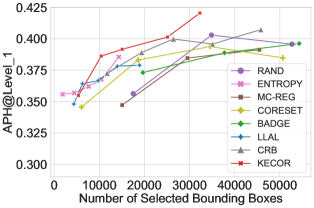
(a)

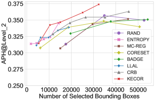
(b)

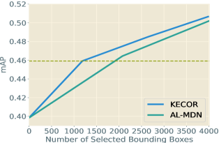
(c)

Figure 4: (a-b) Mean APH scores of Kecor and AL baselines on the Waymo Open val split with Pv-rcnn at the difficulty Level 1 and Level 2, respectively. (c) Performance comparison of 2D object detection on PASCAL VOC07 dataset.

5.2 Baselines

For fair comparisons, eleven active learning baselines are included in our experiments: Rand is a random sampling method selecting $n$ samples. Entropy [61] is an uncertainty-based approach that selects $n$ samples with the highest entropy of predicted labels. Llal [68] is an uncertainty-based method using an auxiliary network to predict indicative loss and select samples that are likely to be mispredicted. Coreset [55] is a diversity-based method that performs core-set selection using a greedy furthest-first search on both labeled and unlabeled embeddings. Badge [5] is a hybrid approach that selects instances that are both diverse and of high magnitude in a hallucinated gradient space. The comparison involved four variants of deep active learning (Mc-mi [18], Mc-reg [41], Crb [41]), and two adapted from 2D detection, Lt/c [30] and Consensus [54]) for 3D detection. Mc-mi used Monte Carlo dropout and mutual information to determine the uncertainty of point clouds, while Mc-reg used $M$-round Mc-dropout to determine regression uncertainty and select top-$n$ samples with the greatest variance for label acquisition. Lt/c measures class-specific localization tightness, while Consensus calculates the variation ratio of minimum IoU value for each RoI-match of 3D boxes. To testify the active learning performance on the 2D detection task, we compare Kecor with Al-mdn [9] approach, which predicts the parameter of Gaussian mixture model and computes epistemic uncertainty as the variance of Gaussian modes.

5.3 Results on KITTI and Waymo Open Datasets

To validate the effectiveness of the proposed Kecor, active learning approaches were evaluated under various settings on the KITTI and Waymo Open datasets.

Results of Pv-rcnn on KITTI. Figure 6 depicts the 3D mAP scores of Pv-rcnn trained by different AL approaches with an increasing number of selected 3D bounding boxes. Specifically, Entropy selects point clouds with the least number of bounding boxes, as higher classification entropy indicates less chance of containing objects in point clouds. To elaborate further, the number of bounding boxes selected by Mc-reg is generally high and of a large variance, as more instances contained in point clouds will trigger higher aleatoric uncertainty in the box regression. It is observed that AL methods Kecor, Crb and Bait which jointly consider aleatoric and epistemic uncertainties, effectively balance between annotation costs and 3D detector performance across all detection difficulty levels. Among these three methods, the proposed Kecor outperforms Crb and Bait, reducing the number of required annotations by 36.8% and 64.0%, respectively, without compromising detection performance. A detailed AP score for each class is reported in Table 1 when the box-level annotation budget is set to 800 (i.e., 1% queried bounding boxes). It is worth noting that the AP scores yield by Kecor are observed to be higher than all other AL baselines. The BEV scores and the detailed analysis are provided in the supplementary material.

Results of Second on KITTI. We further test the active learning performance of one-stage detector Second on the KITTI dataset. Table 2 reports the 3D mAP and BEV mAP scores across different difficulty levels with around 1,400 bounding boxes. A performance gain of Kecor over the state-of-the-art approach Crb is about 3.5% and 2.8% on average with respect to 3D and BEV mAP scores. Figure 3 shows a more intuitive trend that Kecor achieves a higher boost on the recognition mAP at the Moderate and Hard levels. This implies that the incorporated NTK kernel helps capture the objects that are of sparse point clouds and generally hard to learn, which enhances the detector’s capacity on identifying challenging objects.

Results of Pv-rcnn on Waymo Open. To study the scalability and effectiveness of Kecor, we conduct experiments on the large-scale Waymo Open dataset, the results of which are illustrated in Figure 4a and Figure 4b for different difficulty levels. The proposed approach surpasses all existing AL approaches by a large margin, which verifies the validity of the proposed kernel coding rate maximization strategy. Notably, Kecor saves around 44.4% 3D annotations than Crb when reaching the same detection performance.

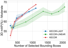
(a)

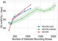
(b)

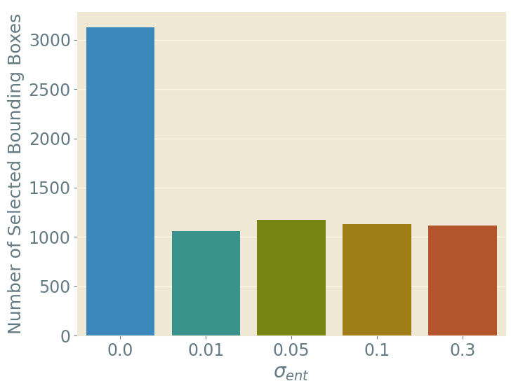
(c)

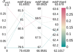
(d)

Figure 5: Ablation studies on the (a-b) impact of kernels in Kecor and (c-d) impact of coefficient $\sigma_{\operatorname{ent}}$ on the KITTI dataset.

5.4 Ablation Study

We conducted a series of experiments to understand the impact of kernels and the coefficient $\sigma_{\operatorname{ent}}$ on the performance of our approach on the KITTI dataset. The central tendency of the performance (e.g., mean mAP) and variations (e.g., error bars) are reported based on outcomes from the two trials for each variant.

5.4.1 Impact of Kernels

We conducted experiments on KITTI to evaluate the effect of kernels on the proposed method, and the active learning results yielded with the Pv-rcnn and Second backbones are reported in Figure 5a and Table 2, respectively. We refer the variants of Kecor with the linear kernel, Laplace RBF kernel, last-layer gradient kernel, and NTK kernel as to Kecor-linear, Kecor-rbf, Kecor-last and Kecor, respectively. Figure 5a shows that Kecor achieves the highest mAP scores ($68.67\%$) among Kecor-linear ($66.82\%$) and Kecor-last ($68.31\%$) at the moderate difficulty level. Regarding the box-level annotation costs, Kecor acquires a comparable amount as Kecor-last, while Kecor-linear requires $1.91$ times more bounding boxes. Table 2 shows that Kecor-last and Kecor gain a relative $7.6\%$ and $5.5\%$ improvement, respectively, over Kecor-linear on the 3D mAP and BEV mAP scores with the Second detector. In particular, Kecor surpasses the variant Kecor-rbf by $2.5\%$ and $1.9\%$ on 3D mAP and BEV mAP, respectively. The performance gains evidence that the applied NTK kernel not only captures the non-linear relationship between the inputs and outputs, but also the aleatoric uncertainty for both tasks.

5.4.2 Impact of Coefficient $\sigma_{\operatorname{ent}}$

We delve into the susceptibility of our method to various values of the coefficient $\sigma_{\operatorname{ent}}$, which varies in $\{0,0.01,0.05,0.1,0.3\}$. The performances of different variants are measured using the mean average precision (mAP) results on the KITTI dataset. The detection performance for the last round and the total amount of queried 3D bounding boxes for each variant are summarized in the barplot (Figure 5c) and the parallel plot (Figure 5d). The results show that different values of $\sigma_{\operatorname{ent}}$ only had a limited impact on the 3D mAP scores, with variations up to $2.8\%$, $3.0\%$ and $2.5\%$ across different difficulty levels, which affirms the resilience of the proposed method to the selection of $\sigma_{\operatorname{ent}}$. Notably, the variant of Kecor without the classification entropy term ($\sigma_{\operatorname{ent}}=0$) produces approximately $3$ times more bounding boxes to annotate than other variants as shown in Figure 5c. We infer this was attributed to the higher entropy of point clouds containing fewer repeated objects, which regularizes the acquisition criteria and ensures a minimal annotation cost. We provide an additional study on the impact of $\sigma_{\operatorname{ent}}$ on the Waymo Open dataset in the supplementary material.

5.5 Analysis on Running Time

To ensure the proposed approach is efficient and reproducible, we have conducted an analysis of the average runtime yielded by the proposed Kecor and the state-of-the-art active 3D detection method Crb on two benchmark datasets, i.e., KITTI and Waymo Open. The training hours of each approach are reported in Table 3. With different choices on base kernels, our finding indicates that Kecor outperforms Crb in terms of running efficiency, achieving a relative improvement of $5.2\%\sim 6.4\%$ on the KITTI dataset and of $24.0\%\sim 26.4\%$ on the large-scale Waymo Open dataset. These results suggest that Kecor is a highly effective and efficient approach for active 3D object detection, especially for large datasets, and has the potential to benefit real-world applications.

Table 3: Running time (hours) comparisons with Pv-rcnn.

AL Strategy	KITTI	Waymo Open	Improvement
Crb	11.935	86.595
Kecor-linear	11.170	63.701	+6.4% / +26.4%
Kecor-last	11.313	64.741	+5.2% / +25.2%
Kecor	11.313	65.782	+5.2% / +24.0%

5.6 Results on 2D Object Detection

To examine the versatility of the proposed Kecor strategy, we conducted additional experiments on the task of 2D object detection. To ensure a fair comparison with Al-mdn [9], we adopt the SSD [38] architecture with VGG16 as the backbone. With a fixed budget for acquiring labeled images, Kecor demonstrates superior performance over Al-mdn in the early cycles as shown in Figure 4c. As the green dotted line indicates, Kecor requires only 1,187 box annotations to achieve the same level of mAP scores, while Al-mdn requires 1,913 annotations, resulting in approximately $38\%$ savings in labeling costs. These results evidence that Kecor effectively trades off between annotation costs and detection performance.

6 Conclusion

This paper studies a novel informative-theoretic acquisition criterion for the active 3D detection task, which well balances a trade-off between the quantity of selected bounding boxes and the yielded detection performance. By maximizing the kernel coding rate, the informative point clouds are identified and selected, which bring in unique and novel knowledge for both 3D box classification and regression. The proposed Kecor is proven to be versatile to one-stage and two-stage detectors and also applicable to 2D object detection tasks. The proposed strategy achieves superior performance on benchmark datasets and also significantly reduces the running time and labeling costs simultaneously.

Appendix A More Discussions on Laplace RBF Kernel

Recall that in Section 4.1, we have discussed that the linear kernel $K_{\operatorname{Linear}}$ can be a useful starting point, it may be necessary to consider other PSD kernels that are better suited to the specific characteristics of the point cloud data at hand. The Laplace Radial Basis Function (RBF) kernel, also known as the Laplacian kernel, is a popular choice of kernel in machine learning algorithms. The Laplace RBF kernel maps the input features into a higher-dimensional feature space, where non-linear relationships can be more easily captured. This kernel function for two latent features $\mathfrak{m}_{i}$ and $\mathfrak{m}_{j}$ can be mathematically represented as follows:

$$K_{\operatorname{RBF}}(\mathfrak{m}_{i},\mathfrak{m}_{j})=\exp(-\frac{\|\mathfrak{m}_{i}-\mathfrak{m}_{j}\|}{\sigma}),$$ (11)

where $\sigma$ indicates a hyperparameter that controls the width of the kernel. $\sigma$ is empirically set to 1.0. The Laplace RBF kernel has a sharp cutoff beyond a distance of $\sigma$, which makes it less sensitive to outliers than the Gaussian RBF kernel. More experimental results and analysis can be found in Section E.

Algorithm 1 The PseudoCode of Kecor.

1:Inputs:

2:      $\mathcal{D}_{L}$: a set of labeled point clouds $\mathcal{D}_{U}$: a set of unlabeled point clouds $\bm{\Omega}$: annotators $B$: a total budget for selection $\bm{g}(\cdot;\bm{\theta}_{g})$: a feature extractor $\bm{h}(\cdot;\bm{\theta}_{h})$: a detector head $\bm{f}(\cdot;\bm{\theta})$: a proxy network of detector head count: a counter of point clouds selected

3:Outputs:

4:      $\bm{g}(\cdot;\bm{\theta}_{g})$: the trained feature extractor $\bm{h}(\cdot;\bm{\theta}_{h})$: the trained detector head

5:count$\leftarrow 0$

6:procedure Pre-train Detector($\bm{g},\bm{h},\bm{f},\mathcal{D}_{L}$)

7:     Train $\bm{g}$ and $\bm{h}$ with detection loss

8:     Train $\bm{f}$ with regression loss $\mathcal{L}$

9:end procedure

10:while count $<B$ do

11:     procedure Active Selection($\bm{g},\bm{f},\mathcal{D}_{U}$)

12:         Extract features and gradients from $\bm{g}$ and $\bm{f}$

13:         Extract classification entropy for $\mathcal{P}\in\mathcal{D}_{U}$

14:         Calculate $K_{\operatorname{NTK}}$ for any subset $\mathcal{D}\subset\mathcal{D}_{U}$

15:         Select the optimal subset $\mathcal{D}_{r}^{*}$ $\triangleright$ refer to Eq. (10)

16:     end procedure

17:     $\mathcal{D}_{U}\leftarrow\mathcal{D}_{U}\backslash\mathcal{D}^{*}_{r}$$\triangleright$ remove the selected subset

18:     $\mathcal{D}_{S}\leftarrow\bm{\Omega}(\mathcal{D}^{*}_{r})$ $\triangleright$ query labels from annotators

19:     $\mathcal{D}_{L}\leftarrow\mathcal{D}_{L}\cup\mathcal{D}_{S}$

20:     count += $n$ $\triangleright$ number of selected data $n=|\mathcal{D}_{r}^{*}|$

21:     procedure Re-train Detector($\bm{g},\bm{h},\bm{f},\mathcal{D}_{L}$)

22:         Train $\bm{g}$ and $\bm{h}$ with detection loss

23:         Train $\bm{f}$ with regression loss $\mathcal{L}$

24:     end procedure

25:end while

Appendix B The Algorithm of Kecor

In this section, we elaborate on the entire workflow of the proposed Kecor approach for active 3D detection. As illustrated in Algorithm 1, the training and selection process includes three stages: (I) detection pre-training with the labeled set (Line 6), (II) active selection (Line 11) from the unlabeled pool, and (III) detection re-training with the updated labeled set (Line 21). Notably, in the pretraining stage, the proxy network is jointly learned to predict the outputs from the detector head $\bm{h}$. The outputs can be ROI (forground confidence) only for Second [63] or with box regression for Pv-rcnn [58]. The training of the proxy network is iterated by 10 and 20 epochs for KITTI and Waymo Open datasets. When the training of the detection model and proxy network converges, we move to the next active selection stage in which $n$ informative point clouds will be selected based on the kernel coding rate maximization criterion presented in Equation (10). The selected point clouds are expected to bring novel and unique knowledge for the following re-training of the detector. The whole process will be gone through multiple times, until the number of selected point clouds reaches the pre-defined budget $B$.

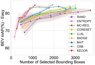
(a)

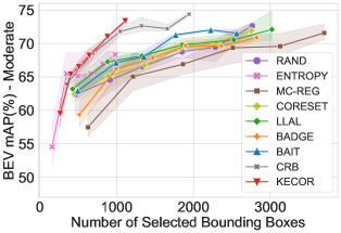
(b)

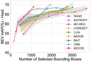
(c)

Figure 6: 3D mAP (%) of Kecor and AL baselines on the KITTI val split with Pv-rcnn.

Appendix C Implementation Details

Following the same setting in [41], the batch sizes for training and evaluation are fixed to 6 and 16 on both KITTI and Waymo Open datasets. The Adam optimizer is adopted with a learning rate initiated as 0.01, and scheduled by one cycle scheduler. The number of Mc-dropout stochastic passes is set to 5.

Active Learning Protocols. For all experiments, we first randomly select $m$ fully labeled point clouds from the training set as the initial $\mathcal{D}_{L}$. With the annotated data, the 3D detector is trained with $E$ epochs, which is then freezed to select $n$ candidates from $\mathcal{D}_{U}$ for label acquisition. We set the $m$ and $n$ to $2.5\sim 3\%$ point clouds (i.e., $n=m=100$ for KITTI, $n=m=400$ for Waymo Open) to trade-off between reliable model training and high computational costs. The aforementioned training and selection steps will alternate for $R$ rounds. Empirically, we set $E=30$, $R=6$ for KITTI, and fix $E=40$, $R=5$ for Waymo Open. All 3D detection experiments are conducted on a GPU cluster with three V100 GPUs and the runs on the VOC07 dataset are conducted on a server with two NVIDIA GeForce RTX 2080 Ti. The runtime for an active learning experiment on KITTI and Waymo is around 11 hours and 65 hours, respectively. Note that, training Pv-rcnn on the full set typically requires 40 GPU hours for KITTI and 800 GPU hours for Waymo.

Appendix D Additional Results on the KITTI Dataset

In this section, we provide an additional study on the BEV mAP scores on the KITTI dataset across different difficulty levels. The detector backbone is set to Pv-rcnn for all AL approaches. The results of the compared AL baselines and the proposed Kecor are plotted in Figure 6. A similar trend is observed to the one shown in Figure 2 in the main body. The proposed Kecor demonstrates a higher performance boost over the state-of-the-art Crb and Bait at the moderate and hard levels.

Appendix E Performance of $K_{\operatorname{RBF}}$ on the KITTI Dataset

To study the performance of the non-linear $K_{\operatorname{RBF}}$, we conducted a series of experiments on the KITTI dataset, with both one-stage and two-stage detectors. The experimental results are shown in Figure 7, where the top row is with Second and the bottom row is with Pv-rcnn, respectively. It can be observed that the Laplace RBF kernel performs better than the linear kernel with Second, yet very similar results with Pv-rcnn. It implies that the one-stage detectors may have a simpler architecture, thus needing the non-linear kernel to help capture the non-linear relationship among the features. However, the performance of Kecor equipped with RBF kernel is still inferior to $K_{\operatorname{Last}}$ and $K_{\operatorname{NTK}}$, which evidence that the empirical NTK kernel can capture not only the non-linear relationship between the inputs and outputs, but also measure the aleatoric uncertainty, thus helping detectors to identify more challenging objects.

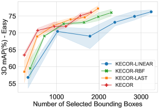
(a)

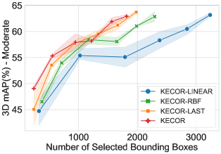
(b)

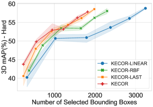
(c)

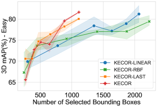
(d)

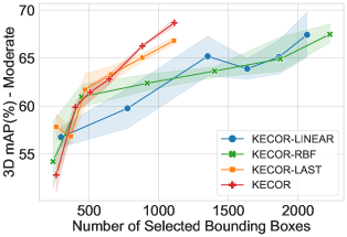
(e)

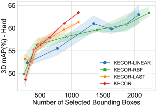
(f)

Figure 7: Ablation study on the different choices of kernels on the KITTI val split with Second (Top row) and Pv-rcnn (Bottom row) across a variety of difficulty levels.

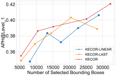
(a)

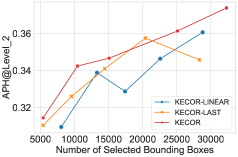
(b)

Figure 8: Ablation study on the different choices of kernels on the Waymo Open dataset with Pv-rcnn.

Appendix F Impact of Kernels on Waymo Open

In addition to the ablation study on KITTI, we also run experiments on the Waymo Open dataset to examine the impact of kernels. The plots are illustrated in Figure 8. Similar to what we observed in KITTI, the Kecor and Kecor-last achieve better performance on both APH at different difficulty levels. However, we also notice that the Kecor-linear does not select too many bounding boxes while it selects 2 times more bounding boxes on the KITTI dataset when reaching the same performance. We reason it is because, in Waymo datasets, most frames of point clouds are densely labeled and there are other irrelevant objects (e.g., signs) that may trigger high entropy scores. Hence, to trade-off between the information and annotation costs, Kecor tends to prefer the point clouds having more information, yielding a slightly higher number of bounding boxes to annotate. How to lower the annotation costs on Waymo will leave an open question in future work.

Appendix G Impact of $\sigma_{\operatorname{ent}}$ on Waymo Open

To study the impact of coefficient $\sigma_{\operatorname{ent}}$ on the Waymo Open dataset, we depict the results in the last round with regard to different evaluation metrics in Figure 9. We run three trials with the values of $\sigma_{\operatorname{ent}}$ varying in $\{0.1,0.5,0.7\}$ considering the high computational costs. The variant of Kecor with the $\sigma_{\operatorname{ent}}=0.7$ achieves the lowest performance. We infer this performance drop is caused by the dominance of the classification entropy regularization term. To trade-off between the high volume of information by kernel coding rate maximization and the lower costs of box annotation by classification entropy regularization, we select 0.5 as the value of $\sigma_{ent}$ for the rest of the experiments on the Waymo Open dataset.

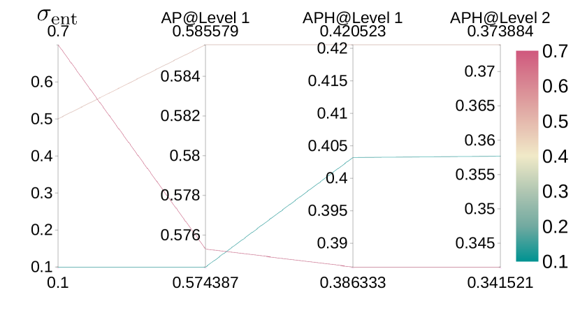
Figure 9: The parallel plot of the impact of $\sigma_{\operatorname{ent}}$ on Waymo.

References

- [1] Sharat Agarwal, Himanshu Arora, Saket Anand, and Chetan Arora. Contextual diversity for active learning. In Proc. European Conference on Computer Vision (ECCV), volume 12361, pages 137–153, 2020.
- [2] Oisin Mac Aodha, Neill D. F. Campbell, Jan Kautz, and Gabriel J. Brostow. Hierarchical subquery evaluation for active learning on a graph. In Proc. IEEE Conference on Computer Vision and Pattern Recognition (CVPR), pages 564–571, 2014.
- [3] Sanjeev Arora, Simon S. Du, Zhiyuan Li, Ruslan Salakhutdinov, Ruosong Wang, and Dingli Yu. Harnessing the power of infinitely wide deep nets on small-data tasks. In Proc. International Conference on Learning Representations (ICLR), 2020.
- [4] Jordan T. Ash, Surbhi Goel, Akshay Krishnamurthy, and Sham M. Kakade. Gone fishing: Neural active learning with fisher embeddings. In Proc. Annual Conference on Neural Information Processing (NeurIPS), pages 8927–8939, 2021.
- [5] Jordan T. Ash, Chicheng Zhang, Akshay Krishnamurthy, John Langford, and Alekh Agarwal. Deep batch active learning by diverse, uncertain gradient lower bounds. In Proc. International Conference on Learning Representations (ICLR), 2020.
- [6] William H. Beluch, Tim Genewein, Andreas Nürnberger, and Jan M. Köhler. The power of ensembles for active learning in image classification. In Proc. IEEE Conference on Computer Vision and Pattern Recognition (CVPR), pages 9368–9377, 2018.
- [7] Shubhang Bhatnagar, Sachin Goyal, Darshan Tank, and Amit Sethi. PAL : Pretext-based active learning. In Proc. British Machine Vision Conference (BMVC), page 195. BMVA Press, 2021.
- [8] Jacob Binia, Moshe Zakai, and Jacob Ziv. On the epsilon -entropy and the rate-distortion function of certain non-gaussian processes. IEEE Transactions on Information Theory, 20(4):517–524, 1974.
- [9] Jiwoong Choi, Ismail Elezi, Hyuk-Jae Lee, Clément Farabet, and Jose M. Alvarez. Active learning for deep object detection via probabilistic modeling. In Proc. International Conference on Computer Vision (ICCV), pages 10244–10253, 2021.
- [10] C. Mario Christoudias, Raquel Urtasun, and Trevor Darrell. Unsupervised feature selection via distributed coding for multi-view object recognition. In Proc. IEEE Conference on Computer Vision and Pattern Recognition (CVPR), 2008.
- [11] Gui Citovsky, Giulia DeSalvo, Claudio Gentile, Lazaros Karydas, Anand Rajagopalan, Afshin Rostamizadeh, and Sanjiv Kumar. Batch active learning at scale. In Proc. Annual Conference on Neural Information Processing (NeurIPS), pages 11933–11944, 2021.
- [12] Thomas M. Cover and Joy A. Thomas. Elements of information theory (2. ed.). 2006.
- [13] Jiajun Deng, Shaoshuai Shi, Peiwei Li, Wengang Zhou, Yanyong Zhang, and Houqiang Li. Voxel R-CNN: towards high performance voxel-based 3d object detection. In Proc. AAAI Conference on Artificial Intelligence (AAAI), pages 1201–1209, 2021.
- [14] Shengheng Deng, Zhihao Liang, Lin Sun, and Kui Jia. VISTA: boosting 3d object detection via dual cross-view spatial attention. In Proc. IEEE Conference on Computer Vision and Pattern Recognition (CVPR), pages 8438–8447. IEEE, 2022.
- [15] Pan Du, Suyun Zhao, Hui Chen, Shuwen Chai, Hong Chen, and Cuiping Li. Contrastive coding for active learning under class distribution mismatch. In Proc. International Conference on Computer Vision (ICCV), pages 8907–8916, 2021.
- [16] Ehsan Elhamifar, Guillermo Sapiro, Allen Y. Yang, and S. Shankar Sastry. A convex optimization framework for active learning. In Proc. International Conference on Computer Vision (ICCV), pages 209–216, 2013.
- [17] M. Everingham, L. Van Gool, C. K. I. Williams, J. Winn, and A. Zisserman. The PASCAL Visual Object Classes Challenge 2007 (VOC2007) Results. http://www.pascal-network.org/challenges/VOC/voc2007/workshop/index.html.
- [18] Di Feng, Xiao Wei, Lars Rosenbaum, Atsuto Maki, and Klaus Dietmayer. Deep active learning for efficient training of a lidar 3d object detector. In Proc. Intelligent Vehicles Symposium, (IV), pages 667–674, 2019.
- [19] Alexander Freytag, Erik Rodner, and Joachim Denzler. Selecting influential examples: Active learning with expected model output changes. In Proc. European Conference on Computer Vision (ECCV), pages 562–577, 2014.
- [20] Yarin Gal and Zoubin Ghahramani. Dropout as a bayesian approximation: Representing model uncertainty in deep learning. In Proc. International Conference on Machine Learning (ICML), volume 48, pages 1050–1059, 2016.
- [21] Andreas Geiger, Philip Lenz, and Raquel Urtasun. Are we ready for autonomous driving? the KITTI vision benchmark suite. In Proc. IEEE Conference on Computer Vision and Pattern Recognition (CVPR), pages 3354–3361, 2012.
- [22] Yuhong Guo. Active instance sampling via matrix partition. In Proc. Annual Conference on Neural Information Processing (NeurIPS), pages 802–810, 2010.
- [23] Ali Harakeh, Michael Smart, and Steven L. Waslander. Bayesod: A bayesian approach for uncertainty estimation in deep object detectors. In Proc. International Conference on Robotics and Automation (ICRA), pages 87–93, 2020.
- [24] Mahmudul Hasan and Amit K. Roy-Chowdhury. Context aware active learning of activity recognition models. In Proc. International Conference on Computer Vision (ICCV), pages 4543–4551, 2015.
- [25] Chenhang He, Ruihuang Li, Shuai Li, and Lei Zhang. Voxel set transformer: A set-to-set approach to 3d object detection from point clouds. In Proc. IEEE Conference on Computer Vision and Pattern Recognition (CVPR), pages 8407–8417. IEEE, 2022.
- [26] Neil Houlsby, Ferenc Huszar, Zoubin Ghahramani, and Máté Lengyel. Bayesian active learning for classification and preference learning. CoRR, abs/1112.5745, 2011.
- [27] Long-Kai Huang, Junzhou Huang, Yu Rong, Qiang Yang, and Ying Wei. Frustratingly easy transferability estimation. In Proc. International Conference on Machine Learning (ICML), volume 162 of Proceedings of Machine Learning Research, pages 9201–9225. PMLR, 2022.
- [28] Arthur Jacot, Clément Hongler, and Franck Gabriel. Neural tangent kernel: Convergence and generalization in neural networks. In Proc. Annual Conference on Neural Information Processing (NeurIPS), pages 8580–8589, 2018.
- [29] Ajay J. Joshi, Fatih Porikli, and Nikolaos Papanikolopoulos. Multi-class active learning for image classification. In Proc. IEEE Conference on Computer Vision and Pattern Recognition (CVPR), pages 2372–2379, 2009.
- [30] Chieh-Chi Kao, Teng-Yok Lee, Pradeep Sen, and Ming-Yu Liu. Localization-aware active learning for object detection. In Proc. Asian Conference on Computer (ACCV), pages 506–522, 2018.
- [31] Kwanyoung Kim, Dongwon Park, Kwang In Kim, and Se Young Chun. Task-aware variational adversarial active learning. In Proc. IEEE Conference on Computer Vision and Pattern Recognition (CVPR), pages 8166–8175, 2021.
- [32] Yoon-Yeong Kim, Kyungwoo Song, JoonHo Jang, and Il-Chul Moon. LADA: look-ahead data acquisition via augmentation for deep active learning. In Proc. Annual Conference on Neural Information Processing (NeurIPS), pages 22919–22930, 2021.
- [33] Andreas Kirsch, Joost van Amersfoort, and Yarin Gal. Batchbald: Efficient and diverse batch acquisition for deep bayesian active learning. In Proc. Annual Conference on Neural Information Processing (NeurIPS), pages 7024–7035, 2019.
- [34] Alex H. Lang, Sourabh Vora, Holger Caesar, Lubing Zhou, Jiong Yang, and Oscar Beijbom. Pointpillars: Fast encoders for object detection from point clouds. In Proc. IEEE Conference on Computer Vision and Pattern Recognition (CVPR), pages 12697–12705. Computer Vision Foundation / IEEE, 2019.
- [35] Jaehoon Lee, Lechao Xiao, Samuel S. Schoenholz, Yasaman Bahri, Roman Novak, Jascha Sohl-Dickstein, and Jeffrey Pennington. Wide neural networks of any depth evolve as linear models under gradient descent. In Neural Tangent Kernel: Convergence and Generalization in Neural Networks, pages 8570–8581, 2019.
- [36] David D. Lewis and Jason Catlett. Heterogeneous uncertainty sampling for supervised learning. In Proc. International Conference on Machine Learning (ICML), pages 148–156, 1994.
- [37] Peng Liu, Lizhe Wang, Rajiv Ranjan, Guojin He, and Lei Zhao. A survey on active deep learning: From model driven to data driven. ACM Computing Surveys, 54(10s):221:1–221:34, 2022.
- [38] Wei Liu, Dragomir Anguelov, Dumitru Erhan, Christian Szegedy, Scott E. Reed, Cheng-Yang Fu, and Alexander C. Berg. SSD: single shot multibox detector. In Proc. European Conference on Computer Vision (ECCV), volume 9905, pages 21–37. Springer, 2016.
- [39] Xin Liu, Zhongdao Wang, Yali Li, and Shengjin Wang. Self-supervised learning via maximum entropy coding. CoRR, abs/2210.11464, 2022.
- [40] Zhuoming Liu, Hao Ding, Huaping Zhong, Weijia Li, Jifeng Dai, and Conghui He. Influence selection for active learning. In Proc. International Conference on Computer Vision (ICCV), pages 9254–9263, 2021.
- [41] Yadan Luo, Zhuoxiao Chen, Zijian Wang, Xin Yu, Zi Huang, and Mahsa Baktashmotlagh. Exploring active 3d object detection from a generalization perspective. In Proc. International Conference on Learning Representations (ICLR), 2023.
- [42] Yi Ma, Harm Derksen, Wei Hong, and John Wright. Segmentation of multivariate mixed data via lossy data coding and compression. IEEE Transactions on Pattern Analysis and Machine Intelligence., 29(9):1546–1562, 2007.
- [43] David J. C. MacKay. Information-based objective functions for active data selection. Journal of Neural Computation, 4(4):590–604, 1992.
- [44] Mohamad Amin Mohamadi, Wonho Bae, and Danica J. Sutherland. Making look-ahead active learning strategies feasible with neural tangent kernels. CoRR, abs/2206.12569, 2022.
- [45] Hieu Tat Nguyen and Arnold W. M. Smeulders. Active learning using pre-clustering. In Carla E. Brodley, editor, Proc. International Conference on Machine Learning (ICML), 2004.
- [46] Roman Novak, Jascha Sohl-Dickstein, and Samuel S. Schoenholz. Fast finite width neural tangent kernel. In Kamalika Chaudhuri, Stefanie Jegelka, Le Song, Csaba Szepesvári, Gang Niu, and Sivan Sabato, editors, Proc. International Conference on Machine Learning (ICML), volume 162, pages 17018–17044. PMLR, 2022.
- [47] Younghyun Park, Soyeong Kim, Wonjeong Choi, Dong-Jun Han, and Jaekyun Moon. Active learning for object detection with evidential deep learning and hierarchical uncertainty aggregation. In Proc. International Conference on Learning Representations (ICLR), 2023.
- [48] Amin Parvaneh, Ehsan Abbasnejad, Damien Teney, Gholamreza (Reza) Haffari, Anton van den Hengel, and Javen Qinfeng Shi. Active learning by feature mixing. In Proc. IEEE Conference on Computer Vision and Pattern Recognition (CVPR), pages 12237–12246, 2022.
- [49] Pengzhen Ren, Yun Xiao, Xiaojun Chang, Po-Yao Huang, Zhihui Li, Brij B. Gupta, Xiaojiang Chen, and Xin Wang. A survey of deep active learning. ACM Computing Surveys, 54(9):180:1–180:40, 2022.
- [50] Dan Roth and Kevin Small. Margin-based active learning for structured output spaces. In Proc. European Conference on Machine Learning (ECML), pages 413–424, 2006.
- [51] Nicholas Roy and Andrew McCallum. Toward optimal active learning through monte carlo estimation of error reduction. In Proc. International Conference on Machine Learning (ICML), pages 441–448, 2001.
- [52] Soumya Roy, Asim Unmesh, and Vinay P. Namboodiri. Deep active learning for object detection. In Proc. British Machine Vision Conference (BMVC), page 91, 2018.
- [53] David Schinagl, Georg Krispel, Horst Possegger, Peter M. Roth, and Horst Bischof. Occam’s laser: Occlusion-based attribution maps for 3d object detectors on lidar data. In Proc. IEEE Conference on Computer Vision and Pattern Recognition (CVPR), pages 1131–1140. IEEE, 2022.
- [54] Sebastian Schmidt, Qing Rao, Julian Tatsch, and Alois C. Knoll. Advanced active learning strategies for object detection. In Proc. Intelligent Vehicles Symposium, (IV), pages 871–876, 2020.
- [55] Ozan Sener and Silvio Savarese. Active learning for convolutional neural networks: A core-set approach. In Proc. International Conference on Learning Representations (ICLR), 2018.
- [56] Burr Settles, Mark Craven, and Soumya Ray. Multiple-instance active learning. In Proc. Annual Conference on Neural Information Processing (NeurIPS), pages 1289–1296, 2007.
- [57] Guangsheng Shi, Ruifeng Li, and Chao Ma. Pillarnet: Real-time and high-performance pillar-based 3d object detection. In Proc. European Conference on Computer Vision (ECCV), volume 13670, pages 35–52, 2022.
- [58] Shaoshuai Shi, Chaoxu Guo, Li Jiang, Zhe Wang, Jianping Shi, Xiaogang Wang, and Hongsheng Li. PV-RCNN: point-voxel feature set abstraction for 3d object detection. In Proc. IEEE Conference on Computer Vision and Pattern Recognition (CVPR), pages 10526–10535, 2020.
- [59] Shaoshuai Shi, Xiaogang Wang, and Hongsheng Li. Pointrcnn: 3d object proposal generation and detection from point cloud. In Proc. IEEE Conference on Computer Vision and Pattern Recognition (CVPR), pages 770–779. Computer Vision Foundation / IEEE, 2019.
- [60] Pei Sun, Henrik Kretzschmar, Xerxes Dotiwalla, Aurelien Chouard, Vijaysai Patnaik, Paul Tsui, James Guo, Yin Zhou, Yuning Chai, Benjamin Caine, Vijay Vasudevan, Wei Han, Jiquan Ngiam, Hang Zhao, Aleksei Timofeev, Scott Ettinger, Maxim Krivokon, Amy Gao, Aditya Joshi, Yu Zhang, Jonathon Shlens, Zhifeng Chen, and Dragomir Anguelov. Scalability in perception for autonomous driving: Waymo open dataset. In Proc. IEEE Conference on Computer Vision and Pattern Recognition (CVPR), pages 2443–2451, 2020.
- [61] Dan Wang and Yi Shang. A new active labeling method for deep learning. In Proc. International Joint Conference on Neural Networks (IJCNN), pages 112–119, 2014.
- [62] Jiaxi Wu, Jiaxin Chen, and Di Huang. Entropy-based active learning for object detection with progressive diversity constraint. In Proc. IEEE Conference on Computer Vision and Pattern Recognition (CVPR), pages 9387–9396. IEEE, 2022.
- [63] Yan Yan, Yuxing Mao, and Bo Li. SECOND: sparsely embedded convolutional detection. Sensors, 18(10):3337, 2018.
- [64] Bin Yang, Wenjie Luo, and Raquel Urtasun. PIXOR: real-time 3d object detection from point clouds. In Proc. IEEE Conference on Computer Vision and Pattern Recognition (CVPR), pages 7652–7660. IEEE, 2018.
- [65] Yi Yang, Zhigang Ma, Feiping Nie, Xiaojun Chang, and Alexander G. Hauptmann. Multi-class active learning by uncertainty sampling with diversity maximization. International Journal of Computer Vision, 113:113–127, 2015.
- [66] Zetong Yang, Yanan Sun, Shu Liu, and Jiaya Jia. 3dssd: Point-based 3d single stage object detector. In Proc. IEEE Conference on Computer Vision and Pattern Recognition (CVPR), pages 11037–11045. Computer Vision Foundation / IEEE, 2020.
- [67] Zetong Yang, Yanan Sun, Shu Liu, Xiaoyong Shen, and Jiaya Jia. STD: sparse-to-dense 3d object detector for point cloud. In Proc. IEEE Conference on Computer Vision and Pattern Recognition (CVPR), pages 1951–1960. IEEE, 2019.
- [68] Donggeun Yoo and In So Kweon. Learning loss for active learning. In Proc. IEEE Conference on Computer Vision and Pattern Recognition (CVPR), pages 93–102, 2019.
- [69] Weiping Yu, Sijie Zhu, Taojiannan Yang, and Chen Chen. Consistency-based active learning for object detection. In Proc. IEEE Conference on Computer Vision and Pattern Recognition Workshops (CVPRW), pages 3950–3959. IEEE, 2022.
- [70] Yaodong Yu, Kwan Ho Ryan Chan, Chong You, Chaobing Song, and Yi Ma. Learning diverse and discriminative representations via the principle of maximal coding rate reduction. In Proc. Annual Conference on Neural Information Processing (NeurIPS), 2020.
- [71] Tianning Yuan, Fang Wan, Mengying Fu, Jianzhuang Liu, Songcen Xu, Xiangyang Ji, and Qixiang Ye. Multiple instance active learning for object detection. In Proc. IEEE Conference on Computer Vision and Pattern Recognition (CVPR), pages 5330–5339, 2021.