Why Does Little Robustness Help? A Further Step Towards Understanding Adversarial Transferability

Abstract

Adversarial examples for deep neural networks (DNNs) have been shown to be transferable: examples that successfully fool one white-box surrogate model can also deceive other black-box models with different architectures. Although a bunch of empirical studies have provided guidance on generating highly transferable adversarial examples, many of these findings fail to be well explained and even lead to confusing or inconsistent advice for practical use.

In this paper, we take a further step towards understanding adversarial transferability, with a particular focus on surrogate aspects. Starting from the intriguing “little robustness” phenomenon, where models adversarially trained with mildly perturbed adversarial samples can serve as better surrogates for transfer attacks, we attribute it to a trade-off between two dominant factors: model smoothness and gradient similarity. Our research focuses on their joint effects on transferability, rather than demonstrating the separate relationships alone. Through a combination of theoretical and empirical analyses, we hypothesize that the data distribution shift induced by off-manifold samples in adversarial training is the reason that impairs gradient similarity.

Building on these insights, we further explore the impacts of prevalent data augmentation and gradient regularization on transferability and analyze how the trade-off manifest in various training methods, thus building a comprehensive blueprint for the regulation mechanisms behind transferability. Finally, we provide a general route for constructing superior surrogates to boost transferability, which optimizes both model smoothness and gradient similarity simultaneously, e.g., the combination of input gradient regularization and sharpness-aware minimization (SAM), validated by extensive experiments. In summary, we call for attention to the united impacts of these two factors for launching effective transfer attacks, rather than optimizing one while ignoring the other, and emphasize the crucial role of manipulating surrogate models.

1 Introduction

Adversarial transferability is an intriguing property of adversarial examples (AEs), where examples crafted against a surrogate DNN could fool other DNNs as well. Various techniques [45, 13, 24, 12, 32, 86, 76, 88, 26] have been proposed for the generation process of AEs to increase transferability, such as integrating momentum to stabilize the update direction [12] or applying transformations at each iteration to create diverse input patterns [76]. At a high level, all these research endeavors to find transferable AEs under given surrogate models by proposing complex tricks to be incorporated into the generation pipeline one after another. However, this approach could result in non-trivial computational expenses and low scalability [49].

With a different perspective, another line of works [22, 23, 72, 34] start to examine the role of surrogate models. One useful observation is that attacking an ensemble of surrogate models with different architectures can obtain a more general update direction for AEs [38, 5]. A recent study [23] also proposed fine-tuning a well-trained surrogate to obtain a set of intermediate models that can be used for an ensemble. However, it remains unclear which type of surrogate performs the best and should be included in the ensemble. Our work taps into this line and tries to manipulate surrogates to launch stronger transfer attacks.

Meanwhile, Demontis et al. [9] started to explain the transferability property and showed that model complexity and gradient alignment negatively and positively correlate with transferability, respectively. Lately, Yang et al. [78] established a transferability lower bound and theoretically connect transferability to two key factors: model smoothness and gradient similarity. Model smoothness captures the general invariance of the gradient w.r.t. input features for a given model, while gradient similarity refers to the alignment of the gradient direction between surrogate and target models. However, there is still much to be understood and explored regarding these factors. For instance, it is unclear which factor plays a more important role in regulating transferability, how existing empirical findings for improving transferability affect these factors, and how to generally optimize them both simultaneously. Such a complex situation makes it challenging to completely understand the role of surrogates. Consequently, there is currently no consensus on how to construct better surrogates to achieve higher adversarial transferability. In support of this, a recent work [42], after performing a large-scale empirical study in real-world settings, concluded that surrogate-level factors that affect the transferability highly chaotically interact and there is no effective solution to obtain a good surrogate except through trial and error.

Table I: The overview of our interactions with literature in the field.

Existing conclusions and viewpoints	Our observations and inferences	Relation
Stronger regularized (smoother) models provide better surrogates on average [9].	(1) AT with large budget yields smoother models that degrade transferability. In Sec. 2.1. (2) Stronger regularizations cannot always outperform less smooth solutions like SAM. In Sec. 4.3.	Partly  conflicting
AT and data augmentation do not show strong correlations to transfer attacks in the “real-world” environment [42].	(1) AT with small budget benefits transfer attack while large budget hinders it. (2) Data augmentation generally impairs transfer attacks, especially for stronger augmentations. In Sec. 6, Q6.	Conflicting
Surrogate models with better generalization performance could result in more transferable AEs [68].	Data augmentations that yield surrogates with the best generalization perform the worst in transfer attacks. In Sec. 6, Q4.	Conflicting
Attacking multiple surrogates from a sufficiently large geometry vicinity (LGV) benefits transferability [23].	Attacking multiple surrogates from arbitrary LGV of a single superior surrogate may degrade transferability. In Sec. 5.2.	Partly  conflicting
Regularizing pressure transfers from the weight space to the input space. [11].	This transfer effect exists, yet is marginal and unstable. In Sec. 4.2.	Partly  conflicting
The poor transferability of ViT is because existing attacks are not strong enough to fully exploit its potential [46].	The transferability of ViT may have been restrained by its default training paradigm. In Sec. 6, Q5	Parallel
Model complexity (the number of local optima in loss surface) correlates with transferability [9].	A smoother model is expected to have less and wider local optima in a finite space. In Sec. 6, Q3	Causal
AEs lie off the underlying manifold of clean data [21].	Adversarial training causes data distribution shift induced by off-manifold AEs, thus impairing gradient similarity.	Dependent
(1) Attacking an ensemble of surrogates in the distribution found by Bayes learning improves the transferability [33]. (2) SAM can be seen as a relaxation of Bayes [44].	SAM yields general input gradient alignment towards every training solution. Attacking SAM solution significantly improves transferability. In Sec. 6, Q7.	Matching

In light of this, we aim to deepen our understanding of adversarial transferability and provide concrete guidelines for constructing better surrogates for improving transferability. Specifically, we offer the following contributions:

Gaining a deeper understanding of the “little robustness” phenomenon. We begin by exploring the intriguing “little robustness” phenomenon [57], where models produced by small-budget adversarial training (AT) serve as better surrogates than standard ones (see Fig. 2). Through tailored definitions of gradient similarity and model smoothness, we recognize this phenomenon comes along with an inherent trade-off effect between these two factors on transferability. Thus we attribute the “little robustness” appearance to the persistent improvement of model smoothness and deterioration of gradient similarity. Further, we identify the observed gradient dissimilarity in AT as the result of the data distribution shift caused by off-manifold samples.

Investigating the impact of data augmentation on transferability. Beyond AT, we explore more general distribution shift cases to confirm our hypothesis on data distribution shift impairing gradient similarity. Specifically, we exploit four popular data augmentation methods, Mixup (MU), Cutmix (CM), Cutout (CO), and Label smoothing (LS) to investigate how these different kinds of distribution shifts affect the gradient similarity. Extensive experiments reveal they unanimously impair gradient similarity in different levels, and the degradation generally aligns with the augmentation magnitude. Moreover, we find different augmentations affect smoothness differently. While LS benefits both datasets, other methods mostly downgrade smoothness in CIFAR-10 and show chaotic performance in ImageNette. Despite their different complex trade-off effects, they consistently yield worse transferability.

Investigating the impact of gradient regularization on transferability. As the concept of gradient similarity is inherently tangled up with unknown target models, it is difficult to directly optimize it in the real scenario. Therefore, we explore solutions that presumably feature better smoothness without explicitly changing the data distribution, i.e., gradient regularization. Concretely, we explore the impact of four gradient regularizations on model smoothness: input gradient regularization (IR) and input Jacobian regularization (JR) in the input space, and explicit gradient regularization (ER) and sharpness-aware minimization (SAM) in the weight space. Our extensive experiments show that gradient regularizations universally improve model smoothness, with regularizations in the input space leading to faster and more stable improvement than regularizations in the weight space. However, while input space regularizations (JR, IR) produce better smoothness, they do not necessarily outperform weight space regularizations like SAM in terms of transferability. We also find this aligns with the fact that they weigh differently on gradient similarity, which plays another crucial role in the overall trade-off.

Proposing a general route for generating surrogates. Considering the practical black-box scenario, we propose a general route for the adversary to obtain surrogates with both superior smoothness and similarity. This involves first assessing the smoothness of different training mechanisms and comparing their similarities, then developing generally effective strategies by combining the best elements of each. Our experimental results show that input regularization and SAM excel at promoting smoothness and similarity, respectively, as well as other complementary properties. Thus, we propose SAM&JR and SAM&IR to obtain better surrogates. Extensive results show our methods significantly outperform existing solutions in boosting transferability. Moreover, we showcase that the design is a plug-and-play method that can be directly integrated with surrogate-independent methods to further improve transferability. The transfer attack results on three commercial Machine-Learning-as-a-Service (MLaaS) platforms also demonstrate the effectiveness of our method against real-world deployed DNNs.

In summary, we study the complex trade-off between model smoothness and gradient similarity (see Fig. 1) under various circumstances and identify a general alignment between the trade-off and transferability. We call for attention that, for effective surrogates, one should handle these two factors well. Throughout our study, we also discover a range of observations correlating existing conclusions and viewpoints in the field, Tab. I provides a glance at them and report the relations.

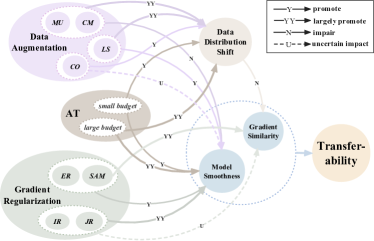
Figure 1: A complete overview of the relationship between factors regulating adversarial transferability of our study.

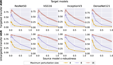
(a) CIFAR-10

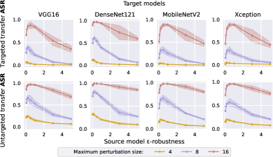
(b) ImageNette

Figure 2: Transfer attack success rates (ASRs) against adversarially trained CIFAR-10 and ImageNette classifiers. We plot the average results of different surrogates obtained by 3 random seeds and the corresponding error bars for each $\epsilon$.

2 Explaining Little Robustness

Understanding adversarial transferability is still a challenging task, and many empirical observations in the literature are rather perplexing. As a typical case, “little robustness” indicates that a model adversarially trained with small perturbation budgets improves the transferability [57, 58]. It remains unclear why small-budget adversarially trained models can serve as better surrogates, whereas large-budget ones do not exhibit this benefit. In this section, we tailor the definitions of gradient similarity and model smoothness, two recently proposed concepts that are believed to be important for transferability [78], to analyze this phenomenon.

Notations. We denote the input space as $\mathcal{X}=\mathbb{R}^{d}$, and the output space as $\mathcal{Y}=\mathbb{R}^{m}$. We also consider a standard classification training dataset $\mathbf{S}=\left\{\left(x_{1},y_{1}\right),\cdots,\left(x_{n},y_{n}\right)\right\}$, where $x_{i}\in\mathcal{M}\subset\mathcal{X}$ and $y_{i}\in\mathcal{L}=\{(0,1)^{m}\}\subset\mathcal{Y}$ are identically and independently distributed (i.i.d.) drawn from the normal data distribution $\mathcal{D}\in\mathcal{P}_{\mathcal{X\times Y}}$. $\mathcal{M}$ denotes the normal (image) feature manifold, $\mathcal{D}$ is supported on $(\mathcal{M},\mathcal{L})$ and $\mathcal{P}_{\mathcal{X\times Y}}$ is the set of distributions on $\mathcal{X\times Y}$. We further denote the marginal distribution on $\mathcal{X}$ and $\mathcal{Y}$ as $\mathcal{P}_{\mathcal{X}}$ and $\mathcal{P}_{\mathcal{Y}}$, respectively. The classification model can be viewed as a mapping function $\mathcal{F}:\mathcal{X}\rightarrow\mathcal{L}$. Specifically, given any input $x\in\mathcal{X}$, $\mathcal{F}$ will find an optimal match $\mathcal{F}(x)=\arg\min_{y\in\mathcal{L}}\ell_{\mathcal{F}}(x,y)$ with the hard labels $\mathcal{L}$, where $\ell_{\mathcal{F}}:\mathcal{X}\times\mathcal{Y}\rightarrow\mathbb{R}_{+}$ can be decomposed to a training loss $\ell$ and the network’s logits output $f(\cdot)$: $\ell_{\mathcal{F}}(x,y):=\ell(f(x),y),(x,y)\in(\mathcal{X},\mathcal{Y}).$

In this paper, we denote the surrogate model and target model as $\mathcal{F}$ and $\mathcal{G}$, respectively. Generally, both $\mathcal{F}$ and $\mathcal{G}$ can be trained within the data distribution $\mathcal{D}$ using $\mathbf{S}$, or a close yet different distribution $\mathcal{D}^{\prime}$ obtained by a specific augmentation mechanism on $\mathbf{S}$. Throughout this paper, we use $\mathcal{D}^{\prime}$ to denote a data distribution different from $\mathcal{D}$. Since this paper focuses on studying the transferability from the surrogate perspective, we assume $\mathcal{G}$ is also well-trained on $\mathcal{D}$ by default. We defer the analysis and results when $\mathcal{G}$ is trained on various $\mathcal{D}^{\prime}$ to Sec. 6, Q2, where the results also support the conclusions drawn from the case of $\mathcal{D}$.

2.1 Transferability Circuit of Adversarial Training

Adversarial training [40] (AT) uses adversarial examples generated on $\mathbf{S}$ as augmented data and minimizes the following adversarial loss:

$$L_{adv}=\frac{1}{\left\|\mathbf{S}\right\|}\sum\limits_{i=1}^{\left\|\mathbf{S}\right\|}\max\limits_{\left\|\delta\right\|_{2}<\epsilon}\ell(f(x_{i}+\delta),y_{i}),$$ (1)

where $\delta\in\mathbb{R}^{d}$ denotes the adversarial perturbation and $\epsilon$ is the adversarial budget. As evidenced by our experiments in Fig. 2, the attack success rates (ASRs) rise with relatively small-budget adversarial trained models and start to decrease with the high-budget ones. This “transferability circuit” is particularly intriguing. We thus revisit the recently proposed transferability lower bound [78] and utilize it as a tool to analyze the underlying reason.

2.2 Lower Bound of Transferability

We first re-define model smoothness, gradient similarity, and the transferability between two models, based on which a lower bound of transferability can be obtained.

Definition 1 (Model smoothness).

Given a model $\mathcal{F}$ and a data distribution $\mathcal{D}$, the smoothness of $\mathcal{F}$ on $\mathcal{D}$ is defined as $\sigma_{\mathcal{F},\mathcal{D}}=\mathbb{E}_{(x,y)\sim\mathcal{D}}[\sigma(\nabla_{x}^{2}\ell_{\mathcal{F}}(x,y))]$, where $\sigma(\cdot)$ denotes the dominant eigenvalue, and $\nabla_{x}^{2}\ell_{\mathcal{F}}(x,y)$ is the Hessian matrix w.r.t. $x$. We abbreviate $\sigma_{\mathcal{F},\mathcal{D}}$ as $\sigma_{\mathcal{F}}$ for simplicity and define the upper smoothness as $\overline{\sigma}_{\mathcal{F}}=\sup\limits_{(x,y)\sim\mathcal{D}}\sigma(\nabla_{x}^{2}\ell_{\mathcal{F}}(x,y))$, where $\sup$ is the supremum function.

A smoother model on $\mathcal{D}$ is featured with smaller $\sigma_{\mathcal{F}}$ and $\overline{\sigma}_{\mathcal{F}}$, indicating more invariance of loss gradient. Different from its original definition where the global Lipschitz constant $\beta_{\mathcal{F}}$ is used [78], we use this curvature metric (i.e., the dominant eigenvalue of the Hessian) to define the model smoothness in a local manner. With this modified definition, we can theoretically and empirically quantify the smoothness of loss surface on $\mathcal{F}$ for a given data distribution $\mathcal{D}$. Moreover, this provides a tighter bound for the model’s loss function gradient, namely, an explicit relation $\overline{\sigma}_{\mathcal{F}}{\color[rgb]{0,0,0}\leq}\beta_{\mathcal{F}}$ holds. Although the true distribution $\mathcal{D}$ is unknown, one can still sample a set of data from $\mathbf{S}$ and use the empirical mean as an approximation to evaluate the model smoothness. Note that our definition is correlated to the model complexity concept introduced in Demontis et al. [9] (see Sec. 6, Q3).

Definition 2 (Gradient similarity).

For two models $\mathcal{F}$ and $\mathcal{G}$ with the loss functions $\ell_{\mathcal{F}}$ and $\ell_{\mathcal{G}}$, the gradient similarity over $(x,y)$ is defined as $\mathcal{S}\left(\ell_{\mathcal{F}},\ell_{\mathcal{G}},x,y\right)=\frac{{\nabla_{x}\ell_{\mathcal{F}}(x,y)}\cdot\nabla_{x}\ell_{\mathcal{G}}(x,y)}{\left\|\nabla_{x}\ell_{\mathcal{F}}(x,y)\right\|_{2}\cdot\left\|\nabla_{x}\ell_{\mathcal{G}}(x,y)\right\|_{2}}.$

Given a distribution $\mathcal{D}$, we can further define the infimum of loss gradient similarity on $\mathcal{D}$ as $\underline{\mathcal{S}}{\color[rgb]{0,0,0}{}_{\mathcal{D}}}\left(\ell_{\mathcal{F}},\ell_{\mathcal{G}}\right)=\inf\limits_{(x,y)\sim\mathcal{D}}\mathcal{S}\left(\ell_{\mathcal{F}},\ell_{\mathcal{G}},x,y\right)$. Similar to Demontis et al. [9], we define the expected loss gradient similarity as $\tilde{\mathcal{S}}{\color[rgb]{0,0,0}{}_{\mathcal{D}}}(\ell_{\mathcal{F}},\ell_{\mathcal{G}})=\mathbb{E}_{(x,y)\sim\mathcal{D}}[\mathcal{S}\left(\ell_{\mathcal{F}},\ell_{\mathcal{G}},x,y\right)]$, which can capture the similarity between two models on $\mathcal{D}$. Naturally, a larger gradient similarity indicates a more general alignment between the adversarial directions of two given models. We can sample a set of data from $\mathbf{S}$ to evaluate this alignment between two models on $\mathcal{D}$.

Definition 3 (Transferability).

Given a normal sample $(x,y)\in\mathcal{D}$, and a perturbed version $x+\delta$ crafted against a surrogate model $\mathcal{F}$. The transferability $T_{r}$ between $\mathcal{F}$ and a target model $\mathcal{G}$ is defined as $T_{r}=\mathbb{I}\left[\mathcal{F}(x)=\mathcal{G}(x)=y\wedge\mathcal{F}\left(x+\delta\right)\neq y\wedge\mathcal{G}\left(x+\delta\right)\neq y\right]$, where $\mathbb{I}$ denotes the indicator function.

Here we define transferability the same way as [78] for untargeted attacks at the instance level. A successful untargeted transfer attack requires both the surrogate and the target models to give correct predictions for the unperturbed input and incorrect predictions for the perturbed one. The targeted version is similar. Note that we abuse the notations $\delta$ and $\epsilon$ in Definitions 3 and 1, while the notations in Eq. 1 have similar meanings under different contexts.

Theorem 1 (Lower bound of transferability).

Given any sample $(x,y)\in\mathcal{D}$, let $x+\delta$ denote a perturbed version of $x$ with fooling probability $\operatorname{Pr}(\mathcal{F}(x+\delta)\neq y)\geq(1-\alpha)$ and perturbation budget $\|\delta\|_{2}\leq\epsilon$. Then the transferability $\operatorname{Pr}\left(T_{r}(\mathcal{F},\mathcal{G},x,y)=1\right)$ between surrogate model $\mathcal{F}$ and target model $\mathcal{G}$ can be lower bounded by
$\operatorname{Pr}\left(T_{r}(\mathcal{F},\mathcal{G},x,y)=1\right)\geq(1-\alpha)-\left(\gamma_{\mathcal{F}}+\gamma_{\mathcal{G}}\right)-\frac{\epsilon(1+\alpha)-c_{\mathcal{F}}(1-\alpha)}{\epsilon-c_{\mathcal{G}}}-\frac{\epsilon(1-\alpha)}{\epsilon-c_{\mathcal{G}}}\sqrt{2-2\underline{\mathcal{S}}_{\mathcal{D}}\left(\ell_{\mathcal{F}},\ell_{\mathcal{G}}\right)}$, where

$$c_{\mathcal{F}} =\min_{(x,y)\sim\mathcal{D}}\frac{\min\limits_{y^{\prime}\in\mathcal{L}:y^{\prime}\neq y}\ell_{\mathcal{F}}\left(x+\delta,y^{\prime}\right)-\ell_{\mathcal{F}}(x,y)-\overline{\sigma}_{\mathcal{F}}\epsilon^{2}/2}{\left\|\nabla_{x}\ell_{\mathcal{F}}(x,y)\right\|_{2}},$$ (2)

$$c_{\mathcal{G}} =\max_{(x,y)\sim\mathcal{D}}\frac{\min\limits_{y^{\prime}\in\mathcal{L}:y^{\prime}\neq y}\ell_{\mathcal{G}}\left(x+\delta,y^{\prime}\right)-\ell_{\mathcal{G}}(x,y)+\overline{\sigma}_{\mathcal{G}}\epsilon^{2}/2}{\left\|\nabla_{x}\ell_{\mathcal{G}}(x,y)\right\|_{2}}.$$

The natural risks (inaccuracy) of models $\mathcal{F}$ and $\mathcal{G}$ on $\mathcal{D}$ are defined as $\gamma_{\mathcal{F}}$ and $\gamma_{\mathcal{G}}$ respectively, and $\overline{\sigma}_{\mathcal{F}}$ and $\overline{\sigma}_{\mathcal{G}}$ are the upper smoothness of $\mathcal{F}$ and $\mathcal{G}$.

Note that we deliver the lower bound of transferability for untargeted attacks as an example, and the targeted attack follows a similar form. The conclusions for the targeted attack agree with the untargeted case, as suggested in [78], so we omit it for space. The proof is provided in the Appendix. Although the theorem is initially for $l_{2}$-norm perturbations, it can be generalized to $l_{\infty}$-norm as demonstrated in [78].

Implications. Different from [78], which seeks to suppress the transferability from both surrogate and target sides, this paper focuses on the surrogate aspect alone to increase transferability. Therefore, we next briefly analyze how all the terms relating to $\mathcal{F}$ influence the lower bound.

• fooling probability $1-\alpha$: this term captures the likelihood of the surrogate $\mathcal{F}$ being fooled by the adversarial instance $x+\delta$. Different AEs generation strategies result in different fooling probabilities. Intuitively, if $x+\delta$ is unable to fool $\mathcal{F}$, we would expect it cannot fool $\mathcal{G}$ as well. The theorem also suggests effective attack strategies to increase the lower bound. Therefore we default to using a strong baseline attack, projected gradient descent (PGD) (Tabs. II and III). We also report the results of AutoAttack (a gradient-based and gradient-free ensemble attack) in the Appendix (Tab. XIII) to ensure the consistency of conclusions.

• natural risk $\gamma_{\mathcal{F}}$: the negative effect of natural risk on the lower bound of transferability is obvious. A model with lame accuracy on $\mathcal{D}$ is certainly undesirable for adversarial attacks. Consequently, we minimize this term by training models with sufficient epochs for CIFAR-10 and fine-tuning pre-trained ImageNet classifiers for ImageNette.

  

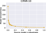
  (a) ResNet18 on CIFAR-10

  

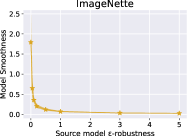
  (b) ResNet50 on ImageNette

  Figure 3: Average model smoothness of $\epsilon$-robust models trained over 3 different random seeds with corresponding error bars at each $\epsilon$. Note that the variances are very small.

• gradient similarity $\underline{\mathcal{S}}_{\mathcal{D}}\left(\ell_{\mathcal{F}},\ell_{\mathcal{G}}\right)$: $\overline{\sigma}_{\mathcal{G}}$ is small compared with the perturbation radius $\epsilon$, and the gradient magnitude $\left\|\nabla_{x}\ell_{\mathcal{G}}\right\|_{2}$ is relatively large, leading to a small $c_{\mathcal{G}}$. Additionally, $1-\alpha$ is large since the attack is generally effective against $\mathcal{F}$. Thus, the right side of the inequality has a form of $C-k\sqrt{1-\underline{\mathcal{S}}_{\mathcal{D}}\left(\ell_{\mathcal{F}},\ell_{\mathcal{G}}\right)}$. Since $C$ and $k$ are both positive, there is a positive relationship between gradient similarity and the lower bound.

• model smoothness $\overline{\sigma}_{\mathcal{F}}$: It’s obvious that a smaller $\overline{\sigma}_{\mathcal{F}}$ generates a larger $c_{\mathcal{F}}$, resulting in a larger lower bound. This indicates smoother models in the input space might serve as better surrogates for transfer attacks.

It is worth noting that a sensible adversary naturally desires to use more precise surrogates and stronger attacks against unknown targets. However, smoothness and similarity are more complex to understand and optimize compared to fooling probability and natural risk. Therefore, we focus on investigating the connection between smoothness, similarity, and transferability as well as how the various training mechanisms regulate them under the restriction that the other two factors above are fairly acceptable. Prior study [9] has shown their link with transferability separately, while we explore their joint effect on transferability.

2.3 Trade-off Under Adversarial Training

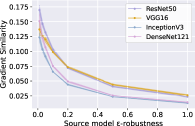
(a) CIFAR-10

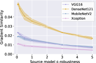
(b) ImageNette

Figure 4: Average gradient similarities between $\epsilon$-robust models and different target models with corresponding error bars at each $\epsilon$ over 3 different random seeds.

Through a combination of theoretical analysis and experimental measurements, here we provide our insights into this “transferability circuit” in adversarial training. Arguably, we make the following two conjectures.

From surrogate’s perspective, the trade-off between model smoothness and gradient similarity can significantly indicate adversarial transferability. First, through mathematical derivation and empirical results, we demonstrate that AT implicitly improves model smoothness. We rewrite the adversarial loss in Eq. 1 as: $\ell(f(x_{i}),y_{i})+[\max\limits_{\left\|\delta\right\|_{2}<\epsilon}\ell(f(x_{i}+\delta),y_{i})-\ell(f(x_{i}),y_{i})]$. The latter term reflects the non-smoothness around point $(x_{i},y_{i})$. Assuming $x_{i}$ is a local minimum of $\ell(f(\cdot),y_{i})$ and applying a Taylor expansion, we get $\max\limits_{\left\|\delta\right\|_{2}\leq\epsilon}\ell(f(x_{i}+\delta),y_{i})-\ell(f(x_{i}),y_{i})=\frac{1}{2}\sigma(\nabla{x}^{2}\ell(f(x_{i}),y_{i}))\cdot\|\delta\|_{2}^{2}+O(\|\delta\|_{2}^{3})$ since the first-order term is 0 at a local minimum. Therefore, AT implicitly penalizes the curvature of $\ell(f(x_{i}),y_{i})$ with a penalty proportional to the norm of adversarial noise $\|\delta\|_{2}^{2}$.

Accordingly, a larger $\epsilon$ strengthens the effect of producing models with greater smoothness. Fig. 3 shows the mean dominant eigenvalues of the Hessian for AT models under various perturbation budgets. It reveals that AT consistently suppresses the dominant eigenvalue, stably producing smoother models. On the other hand, we empirically find that AT impairs gradient similarity. Fig. 4 shows the decay of similarity between surrogate and target models as the budget increases. Notably, for each dataset, smoothness rapidly improves for small $\epsilon$ (as shown by the steep slope in Fig. 3), while gradient similarity gradually decreases. For larger $\epsilon$, improvements in smoothness become marginal since the models are already very smooth. As a reminder, we have controlled the other two terms to be reasonably acceptable. These suggest that:

• The quick improvement in transferability for small $\epsilon$ occurs could be the cause of the rapid gains in smoothness and small decays in gradient similarity.

• The degradation in transferability for large $\epsilon$ occurs may because the smoothness gains have approached the limit while gradient similarity continues to decrease.

Table II: Untargeted and targeted transfer ASRs of AEs crafted against baseline (ST), data augmentations, adversarial training, and gradient regularizations surrogates under the different $L_{\infty}$ budgets (4/255, 8/255, 16/255) on CIFAR-10 using PGD. Results in gray are (more than 0.2%) below the baseline, results in white are close to the baseline ($\pm 0.2\%$). Results in darkest orange are the highest in each respective column, the second darkest are the second highest, and the least dark are others more than 0.2% above the baseline. We conduct experiments using surrogate models trained from 3 different random seeds in each setting and report the average results and the according error bars. In %.

Untargeted
	4/255				8/255				16/255
	ResNet50	VGG16	InceptionV3	DenseNet121	ResNet50	VGG16	InceptionV3	DenseNet121	ResNet50	VGG16	InceptionV3	DenseNet121
ST	54.3±2.9	42.3±1.9	53.6±2.3	70.7±2.0	79.9±3.4	71.4±3.5	80.1±3.2	93.0±1.2	92.8±1.6	90.6±1.9	93.3±2.2	98.6±0.5
MU, $\tau=1$	34.7±2.6	26.7±1.1	35.8±1.8	47.1±3.0	57.1±3.6	49.1±2.2	59.2±2.6	74.0±2.8	76.6±4.1	75.2±3.4	79.9±2.5	90.2±2.4
MU, $\tau=5$	18.5±0.5	15.5±0.2	19.6±0.3	22.8±0.5	31.3±1.7	27.6±0.7	34.5±0.7	40.7±1.2	49.9±1.5	49.1±0.9	54.4±0.3	62.8±1.2
CM, $\tau=1$	29.3±1.2	21.3±0.5	28.4±2.1	39.8±2.0	46.4±2.5	37.6±1.4	45.6±3.2	62.8±2.4	63.3±2.6	60.2±1.4	63.9±3.2	81.1±1.2
CM, $\tau=5$	13.5±0.3	10.8±0.1	13.1±0.4	15.1±0.3	19.5±0.4	15.7±0.2	18.7±0.8	22.6±0.7	29.4±1.4	28.6±1.0	29.3±1.1	34.3±1.5
CO, $\tau=1$	51.5±2.3	41.3±2.4	50.0±1.8	67.7±1.4	78.7±2.4	71.9±3.2	78.2±0.9	92.3±0.9	93.0±2.1	91.8±1.5	93.6±0.7	98.9±0.2
CO, $\tau=5$	37.7±2.8	26.9±1.7	36.9±2.0	49.5±1.2	63.9±4.5	53.1±3.6	64.1±3.9	80.4±1.1	84.7±3.3	79.1±3.5	85.5±3.2	95.3±1.0
LS, $\tau=1$	33.4±1.7	28.6±1.4	33.2±0.6	43.4±1.5	47.5±2.0	44.8±1.1	47.6±0.8	61.8±1.9	59.9±1.5	63.0±1.1	62.9±1.0	75.8±1.4
LS, $\tau=5$	32.8±0.5	28.0±1.3	31.9±0.7	40.8±1.8	50.7±1.4	46.8±2.4	50.6±0.6	63.4±0.9	65.3±2.1	66.1±1.9	66.7±0.5	78.0±0.7
AT	59.0±3.0	50.3±4.4	53.3±2.9	65.3±2.7	87.8±2.8	82.7±4.5	84.7±2.7	92.2±0.8	96.9±1.3	95.8±2.0	96.0±1.4	98.6±0.3
IR	62.3±1.2	55.6±0.5	56.5±2.1	63.7±1.9	96.0±0.4	93.2±0.2	93.8±0.6	96.9±0.6	99.9±0.0	99.7±0.0	99.8±0.1	99.9±0.1
JR	74.2±2.0	65.8±0.8	72.6±0.3	84.1±0.5	94.1±0.7	91.3±0.3	93.4±0.6	97.7±0.5	98.3±0.3	98.3±0.2	98.5±0.4	99.7±0.5
ER	64.9±3.3	52.5±1.9	54.2±6.7	62.8±10.9	94.2±1.4	87.1±5.3	87.9±4.7	92.8±5.3	99.6±0.2	98.7±4.0	98.6±0.8	99.5±0.6
SAM	76.1±1.5	64.3±2.1	74.5±0.7	88.5±0.4	97.5±0.5	94.1±0.8	97.1±0.1	99.6±0.1	99.8±0.0	99.7±0.1	99.9±0.0	100.0±0.0
SAM&IR	64.7±0.3	58.2±0.4	58.4±1.6	65.4±1.0	97.6±0.0	95.5±0.1	95.9±0.4	97.9±0.3	100.0±0.0	99.9±0.0	100.0±0.0	100.0±0.0
SAM&JR	83.1±0.6	70.1±0.9	79.4±0.6	91.5±0.3	98.6±0.2	96.6±0.2	98.3±0.1	99.9±0.0	99.9±0.0	99.9±0.0	99.9±0.0	100.0±0.0
Targeted
ST	18.3±1.4	12.7±0.6	20.4±1.1	34.9±1.9	39.4±4.9	32.7±3.6	43.6±4.0	68.8±4.0	55.7±6.0	53.5±5.5	60.0±5.3	85.4±4.2
MU, $\tau=1$	8.2±0.8	5.9±0.5	10.5±0.6	15.9±1.0	17.0±2.7	13.8±1.4	20.7±2.1	33.3±3.5	28.0±5.1	26.8±2.9	33.1±3.5	50.9±6.2
MU, $\tau=5$	3.0±0.1	2.4±0.1	4.1±0.1	5.0±0.2	6.1±0.5	5.0±0.4	7.9±0.5	10.4±0.5	10.8±0.5	10.7±0.6	13.5±0.6	16.9±0.9
CM, $\tau=1$	6.0±0.4	4.2±0.2	6.8±1.0	11.4±1.1	10.7±0.7	8.3±0.5	11.6±1.8	20.8±1.9	16.4±0.9	14.9±0.8	17.3±2.5	29.6±1.7
CM, $\tau=5$	2.0±0.1	1.6±0.1	2.4±0.2	2.8±0.2	2.8±0.1	2.3±0.0	3.2±0.1	3.7±0.1	4.2±0.2	3.9±0.4	4.4±0.2	4.7±0.3
CO, $\tau=1$	16.0±1.3	11.3±1.2	17.6±1.1	30.6±1.7	35.8±3.0	30.7±2.5	38.6±2.7	63.4±2.2	52.8±4.3	51.5±3.0	55.9±3.1	82.1±1.6
CO, $\tau=5$	7.9±1.1	5.4±0.5	9.5±0.7	14.2±0.7	17.4±2.9	13.6±1.3	20.5±2.1	31.1±0.9	29.1±5.0	24.9±2.8	31.9±4.1	48.5±1.8
LS, $\tau=1$	6.8±0.6	5.4±0.4	7.0±0.3	10.7±1.3	9.9±3.8	9.0±4.0	10.0±3.3	15.6±6.2	15.4±1.9	16.7±1.8	16.3±1.2	23.9±2.9
LS, $\tau=5$	6.7±0.4	5.7±0.1	7.1±0.8	10.5±1.3	13.5±1.1	12.8±0.7	14.0±1.5	20.1±2.0	19.4±0.9	20.0±0.3	20.0±1.4	27.0±1.8
AT	24.9±2.2	18.6±3.4	21.9±2.0	32.5±2.5	60.7±6.7	52.4±7.9	55.6±5.5	72.6±4.0	77.4±7.7	74.6±7.9	72.4±6.7	88.4±4.1
IR	25.7±1.1	20.6±0.2	22.5±1.1	28.8±1.3	70.8±0.5	62.8±0.7	65.0±1.5	75.2±0.6	89.9±0.7	86.7±0.8	86.3±1.3	92.7±0.8
JR	38.6±2.6	30.3±1.2	39.1±0.1	54.0±1.2	75.2±3.9	69.6±2.5	76.0±0.9	90.0±0.8	87.3±2.8	88.9±1.8	88.4±1.0	97.6±0.3
ER	22.7±1.6	15.5±2.8	17.8±3.4	24.1±8.1	54.6±3.3	42.7±6.9	44.1±8.0	55.0±15.9	77.2±3.0	67.2±8.3	66.5±9.6	76.6±16.7
SAM	35.0±1.9	25.2±1.8	36.9±1.3	56.7±0.2	74.7±3.1	65.7±3.5	76.5±1.9	94.0±0.4	92.3±1.5	90.9±2.2	93.4±0.3	99.5±0.2
SAM&IR	28.6±0.2	23.5±0.2	25.0±1.2	31.4±0.7	81.8±0.0	75.7±0.2	77.6±1.1	84.8±0.6	99.2±0.1	98.7±0.1	98.6±0.4	99.6±0.1
SAM&JR	44.2±1.5	32.9±1.1	46.1±1.3	65.7±0.3	85.5±1.4	77.6±1.7	87.3±1.4	97.6±0.1	98.3±0.5	97.5±0.4	98.6±0.4	99.9±0.0

Based on the above analyses, we can infer that the “transferability circuit” of AT may primarily arise from the trade-off effect between smoothness and similarity, given the restriction of surrogates with relatively good accuracies and a highly effective attack strategy. This inference is intuitively inspired by the implications regarding all the surrogate-related factors in Theorem 1.

Meanwhile, we observe that the “transferability circuit” of AT generally exists, though it varies under different non-surrogate circumstances. For example, the optimal $\epsilon$ AT to achieve the best ASRs varies among datasets and perturbation budgets in Fig. 2. This suggests that for different non-surrogate factors, the extent to which model smoothness and gradient similarity contribute to transferability may vary.

Consequently, we make the conjecture that when generating AEs against accurate surrogate models using effective strategies, the trade-off between model smoothness and gradient similarity is strongly correlated with the transferability of those examples from the surrogate models. To test this conjecture, we will investigate changes in model smoothness and gradient similarity alongside the corresponding transfer ASRs under various surrogate training mechanisms in Secs. 3 and 4. Furthermore, in Sec. 6, Q1, we provide a statistical analysis of the correlations between model smoothness, gradient similarity and transferability. Moving forward, the primary concern at hand is to ascertain the rationale of this similarity deterioration in AT, as well as how to generally avoid this and reach a better balance of smoothness and similarity for stronger transfer attacks.

Table III: Transfer ASRs of AEs on ImageNette using PGD. We plot this table in the same way as Tab. II. In %.

Untargeted
	4/255				8/255				16/255
	VGG16	DenseNet121	MobileNetV2	Xception	VGG16	DenseNet121	MobileNetV2	Xception	VGG16	DenseNet121	MobileNetV2	Xception
ST	$\textrm{11.2}_{\pm 1.0}$	$\textrm{17.5}_{\pm 1.1}$	$\textrm{7.6}_{\pm 0.4}$	$\textrm{8.7}_{\pm 0.5}$	$\textrm{28.7}_{\pm 1.1}$	$\textrm{42.7}_{\pm 3.5}$	$\textrm{18.3}_{\pm 0.7}$	$\textrm{18.5}_{\pm 1.3}$	$\textrm{61.7}_{\pm 4.7}$	$\textrm{81.4}_{\pm 4.6}$	$\textrm{49.3}_{\pm 2.7}$	$\textrm{44.1}_{\pm 5.1}$
MU, $\tau=1$	$\textrm{9.2}_{\pm 1.6}$	$\textrm{12.7}_{\pm 0.9}$	$\textrm{7.2}_{\pm 0.6}$	$\textrm{7.2}_{\pm 0.2}$	$\textrm{20.7}_{\pm 1.3}$	$\textrm{22.7}_{\pm 1.3}$	$\textrm{13.7}_{\pm 1.5}$	$\textrm{12.7}_{\pm 1.1}$	$\textrm{43.9}_{\pm 2.3}$	$\textrm{53.3}_{\pm 4.1}$	$\textrm{38.3}_{\pm 3.1}$	$\textrm{29.3}_{\pm 2.9}$
MU, $\tau=5$	$\textrm{6.7}_{\pm 1.1}$	$\textrm{6.7}_{\pm 0.9}$	$\textrm{5.1}_{\pm 0.5}$	$\textrm{5.7}_{\pm 0.5}$	$\textrm{11.5}_{\pm 0.5}$	$\textrm{12.0}_{\pm 0.6}$	$\textrm{8.1}_{\pm 0.7}$	$\textrm{8.1}_{\pm 0.1}$	$\textrm{29.3}_{\pm 0.7}$	$\textrm{29.2}_{\pm 2.4}$	$\textrm{24.1}_{\pm 1.3}$	$\textrm{18.8}_{\pm 0.2}$
CM, $\tau=1$	$\textrm{7.8}_{\pm 0.6}$	$\textrm{10.6}_{\pm 1.0}$	$\textrm{6.1}_{\pm 0.7}$	$\textrm{7.1}_{\pm 0.5}$	$\textrm{16.5}_{\pm 1.3}$	$\textrm{18.1}_{\pm 1.7}$	$\textrm{10.3}_{\pm 0.3}$	$\textrm{10.3}_{\pm 0.1}$	$\textrm{35.8}_{\pm 1.0}$	$\textrm{42.6}_{\pm 2.4}$	$\textrm{29.6}_{\pm 2.0}$	$\textrm{21.5}_{\pm 0.5}$
CM, $\tau=5$	$\textrm{5.5}_{\pm 0.5}$	$\textrm{6.3}_{\pm 0.1}$	$\textrm{4.2}_{\pm 0.4}$	$\textrm{4.6}_{\pm 0.4}$	$\textrm{8.9}_{\pm 0.9}$	$\textrm{9.3}_{\pm 0.3}$	$\textrm{6.7}_{\pm 0.3}$	$\textrm{6.7}_{\pm 0.5}$	$\textrm{19.3}_{\pm 0.5}$	$\textrm{18.3}_{\pm 1.1}$	$\textrm{17.0}_{\pm 0.6}$	$\textrm{11.7}_{\pm 0.5}$
CO, $\tau=1$	$\textrm{11.8}_{\pm 0.4}$	$\textrm{16.7}_{\pm 1.1}$	$\textrm{8.1}_{\pm 0.5}$	$\textrm{8.7}_{\pm 0.3}$	$\textrm{28.3}_{\pm 1.1}$	$\textrm{40.5}_{\pm 2.9}$	$\textrm{18.5}_{\pm 0.7}$	$\textrm{18.4}_{\pm 1.4}$	$\textrm{61.8}_{\pm 1.4}$	$\textrm{79.8}_{\pm 2.4}$	$\textrm{50.9}_{\pm 1.9}$	$\textrm{43.8}_{\pm 0.6}$
CO, $\tau=5$	$\textrm{10.3}_{\pm 0.7}$	$\textrm{14.3}_{\pm 0.3}$	$\textrm{7.3}_{\pm 0.9}$	$\textrm{7.7}_{\pm 0.7}$	$\textrm{25.1}_{\pm 1.7}$	$\textrm{34.5}_{\pm 2.3}$	$\textrm{17.3}_{\pm 1.9}$	$\textrm{15.9}_{\pm 1.1}$	$\textrm{56.4}_{\pm 4.2}$	$\textrm{75.0}_{\pm 3.6}$	$\textrm{46.3}_{\pm 0.9}$	$\textrm{40.1}_{\pm 2.1}$
LS, $\tau=1$	$\textrm{6.8}_{\pm 0.6}$	$\textrm{8.7}_{\pm 0.3}$	$\textrm{5.2}_{\pm 0.4}$	$\textrm{5.9}_{\pm 0.9}$	$\textrm{13.2}_{\pm 0.6}$	$\textrm{14.7}_{\pm 0.1}$	$\textrm{9.5}_{\pm 0.1}$	$\textrm{8.5}_{\pm 0.5}$	$\textrm{27.6}_{\pm 0.2}$	$\textrm{35.5}_{\pm 0.7}$	$\textrm{24.8}_{\pm 0.8}$	$\textrm{18.0}_{\pm 0.6}$
LS, $\tau=5$	$\textrm{6.1}_{\pm 0.3}$	$\textrm{7.1}_{\pm 0.5}$	$\textrm{4.7}_{\pm 0.5}$	$\textrm{5.5}_{\pm 0.5}$	$\textrm{9.1}_{\pm 1.1}$	$\textrm{10.2}_{\pm 0.8}$	$\textrm{7.2}_{\pm 0.2}$	$\textrm{7.8}_{\pm 0.2}$	$\textrm{20.0}_{\pm 1.2}$	$\textrm{23.1}_{\pm 1.3}$	$\textrm{18.6}_{\pm 1.6}$	$\textrm{14.4}_{\pm 0.8}$
AT	$\textrm{14.7}_{\pm 2.1}$	$\textrm{20.5}_{\pm 1.5}$	$\textrm{15.3}_{\pm 1.3}$	$\textrm{15.7}_{\pm 0.9}$	$\textrm{52.1}_{\pm 6.3}$	$\textrm{68.7}_{\pm 2.9}$	$\textrm{59.3}_{\pm 7.1}$	$\textrm{52.3}_{\pm 5.1}$	$\textrm{96.5}_{\pm 1.5}$	$\textrm{98.8}_{\pm 0.4}$	$\textrm{97.5}_{\pm 0.5}$	$\textrm{95.7}_{\pm 0.9}$
IR	$\textrm{21.0}_{\pm 6.6}$	$\textrm{31.7}_{\pm 6.9}$	$\textrm{18.5}_{\pm 5.1}$	$\textrm{19.5}_{\pm 4.3}$	$\textrm{62.5}_{\pm 14.3}$	$\textrm{85.6}_{\pm 9.0}$	$\textrm{65.2}_{\pm 16.4}$	$\textrm{58.4}_{\pm 14.0}$	$\textrm{94.7}_{\pm 6.9}$	$\textrm{99.5}_{\pm 0.3}$	$\textrm{95.7}_{\pm 5.3}$	$\textrm{94.6}_{\pm 5.0}$
JR	$\textrm{26.3}_{\pm 2.1}$	$\textrm{37.3}_{\pm 0.7}$	$\textrm{21.7}_{\pm 1.3}$	$\textrm{20.5}_{\pm 1.3}$	$\textrm{68.5}_{\pm 2.1}$	$\textrm{87.0}_{\pm 0.2}$	$\textrm{67.6}_{\pm 3.6}$	$\textrm{56.0}_{\pm 5.6}$	$\textrm{95.0}_{\pm 1.4}$	$\textrm{99.5}_{\pm 0.1}$	$\textrm{94.7}_{\pm 1.1}$	$\textrm{89.8}_{\pm 3.0}$
ER	$\textrm{13.2}_{\pm 2.8}$	$\textrm{20.9}_{\pm 1.7}$	$\textrm{8.9}_{\pm 1.5}$	$\textrm{9.6}_{\pm 1.0}$	$\textrm{33.3}_{\pm 9.9}$	$\textrm{51.1}_{\pm 8.7}$	$\textrm{20.7}_{\pm 3.7}$	$\textrm{20.5}_{\pm 3.3}$	$\textrm{67.5}_{\pm 15.9}$	$\textrm{89.3}_{\pm 6.7}$	$\textrm{54.5}_{\pm 9.1}$	$\textrm{50.1}_{\pm 8.7}$
SAM	$\textrm{22.8}_{\pm 1.4}$	$\textrm{29.7}_{\pm 1.5}$	$\textrm{12.8}_{\pm 0.8}$	$\textrm{12.8}_{\pm 0.0}$	$\textrm{58.7}_{\pm 2.7}$	$\textrm{72.8}_{\pm 2.0}$	$\textrm{42.3}_{\pm 1.1}$	$\textrm{34.7}_{\pm 1.7}$	$\textrm{91.4}_{\pm 2.0}$	$\textrm{97.1}_{\pm 0.3}$	$\textrm{81.0}_{\pm 1.8}$	$\textrm{75.3}_{\pm 1.7}$
SAM&IR	$\textrm{26.9}_{\pm 5.5}$	$\textrm{39.8}_{\pm 4.8}$	$\textrm{24.3}_{\pm 4.7}$	$\textrm{23.2}_{\pm 4.0}$	$\textrm{72.5}_{\pm 10.9}$	$\textrm{92.6}_{\pm 2.8}$	$\textrm{78.5}_{\pm 9.5}$	$\textrm{68.9}_{\pm 10.3}$	$\textrm{98.1}_{\pm 2.1}$	$\textrm{99.8}_{\pm 0.2}$	$\textrm{98.7}_{\pm 1.5}$	$\textrm{97.7}_{\pm 2.3}$
SAM&JR	$\textrm{32.7}_{\pm 4.3}$	$\textrm{46.3}_{\pm 3.7}$	$\textrm{28.1}_{\pm 4.5}$	$\textrm{24.9}_{\pm 4.1}$	$\textrm{76.6}_{\pm 5.6}$	$\textrm{93.6}_{\pm 1.2}$	$\textrm{73.1}_{\pm 7.7}$	$\textrm{65.9}_{\pm 7.7}$	$\textrm{96.7}_{\pm 7.3}$	$\textrm{99.8}_{\pm 0.2}$	$\textrm{96.6}_{\pm 1.6}$	$\textrm{93.9}_{\pm 4.1}$
Targeted
ST	2.1±0.3	4.1±0.3	0.6±0.4	2.0±0.2	10.4±0.8	19.6±2.8	4.2±0.4	5.7±1.7	33.6±3.8	60.3±7.5	19.5±2.1	19.7±3.1
MU, $\tau=1$	1.3±0.3	2.3±0.3	0.4±0.2	1.0±0.2	5.1±0.7	7.3±1.1	1.5±0.3	2.5±0.1	15.7±1.9	25.1±4.1	9.3±1.5	8.8±2.4
MU, $\tau=5$	0.9±0.1	0.6±0.0	0.1±0.1	0.5±0.1	1.3±0.3	1.1±0.1	0.4±0.4	1.0±0.2	3.8±0.8	3.7±0.7	1.7±0.1	2.8±0.6
CM, $\tau=1$	1.1±0.5	1.4±0.2	0.2±0.2	0.7±0.3	2.3±0.3	3.1±0.5	0.7±0.1	1.7±0.5	6.5±0.5	9.4±0.4	3.7±0.3	4.9±0.3
CM, $\tau=5$	0.7±0.1	0.8±0.0	0.1±0.1	0.4±0.2	0.9±0.3	1.0±0.2	0.2±0.2	0.9±0.1	2.3±0.3	2.5±0.1	1.4±0.4	1.6±0.2
CO, $\tau=1$	2.3±0.5	3.4±0.6	0.4±0.2	1.7±0.3	9.3±1.3	18.2±3.0	3.2±1.0	4.9±0.5	31.0±2.4	62.3±6.9	18.2±1.6	17.4±1.8
CO, $\tau=5$	1.9±0.1	3.1±0.9	0.6±0.2	1.2±0.2	8.8±1.4	14.9±0.9	3.8±1.0	4.3±1.1	28.3±2.9	52.5±2.1	16.2±3.0	16.9±1.3
LS, $\tau=1$	0.9±0.1	1.5±0.5	0.4±0.0	0.7±0.1	1.6±0.0	2.5±0.1	0.5±0.1	1.4±0.2	4.0±0.2	6.3±0.7	3.2±0.6	2.8±0.2
LS, $\tau=5$	0.7±0.1	1.2±0.0	0.3±0.1	0.5±0.3	1.2±0.0	1.9±0.5	0.3±0.1	1.0±0.2	2.7±0.9	3.7±0.9	2.2±0.4	2.3±0.7
AT	2.1±0.9	4.0±0.8	1.1±0.3	2.6±0.2	22.5±3.1	39.3±2.9	26.2±5.4	25.1±4.1	84.7±3.7	94.1±1.5	88.3±2.2	89.3±2.5
IR	4.2±2.0	9.9±3.7	3.4±1.6	3.3±1.1	33.6±13.4	65.3±14.3	34.1±12.7	31.9±13.5	84.5±14.3	98.2±2.2	86.9±12.3	84.6±14.6
JR	6.5±0.5	14.0±0.8	4.6±0.4	4.8±0.6	41.4±5.2	71.7±2.5	36.5±5.7	33.6±5.8	82.5±7.3	98.1±1.3	79.5±6.7	76.0±9.4
ER	2.6±0.8	5.9±1.5	0.7±0.3	1.9±0.3	12.3±5.7	26.7±8.1	4.7±1.5	6.7±2.5	40.4±20.8	75.0±12.8	23.5±9.9	24.6±10.8
SAM	6.1±1.1	8.9±0.9	2.3±0.5	3.3±0.1	28.1±1.1	46.5±1.3	12.6±2.0	11.6±0.8	76.0±0.4	92.1±1.1	52.4±1.0	53.7±1.3
SAM&IR	5.9±2.1	13.2±2.8	5.2±1.6	4.3±0.9	44.2±12.8	76.3±4.5	46.5±12.1	43.6±11.8	92.5±6.7	99.5±0.1	93.5±4.5	92.4±4.8
SAM&JR	9.9±1.3	19.5±1.3	6.4±0.6	5.9±1.1	50.0±6.4	78.7±1.7	41.4±9.0	38.4±7.2	88.7±7.5	99.3±0.1	83.1±5.7	84.1±7.1

Data distribution shift impairs gradient similarity. Different from model smoothness, it is difficult to understand how exactly AT degrades the gradient similarity. In this work, we attribute this degradation to the data distribution shift induced by the off-manifold examples in AT. Since the emerging of adversarial examples [61], there is a long-held belief that: Clean data lies in a low-dimensional manifold. Even though the adversarial examples are close to the clean data, they lie off the underlying data manifold [39, 56, 30, 21, 37]. Nevertheless, recent researches demonstrate that AEs can also be on-manifold [31, 48, 59, 36, 37], and on-manifold and off-manifold AEs may co-exist [75]. With this in mind, we analyze how AT enlarges the data distribution shift along with the increment of adversarial budget $\epsilon$.

Given a regular loss function $\ell(f(x),y)$ on the low-dimensional manifold $\mathcal{M}$, the adversarial perturbation $\delta\in\mathbb{R}^{d}$ could make the loss $\ell(f(x+\delta),y)$ sufficiently high with $x+\delta\in\mathcal{M}$ or $x+\delta\notin\mathcal{M}$ [77]. At a high level, AT augments the dataset by adding adversarial examples during each iteration, obtaining an augmented data distribution on $\mathcal{P}_{\mathcal{X}}$, and the adversarial budget $\epsilon$ can be regarded as a parameter that controls the augmentation magnitude. Intuitively, a larger $\epsilon$ induces more space for off-manifold samples, resulting in a larger distribution shift. On the other hand, it is also widely acknowledged that adversarial training with larger perturbation budgets leads to robust overfitting [73, 14, 60, 50]. Accordingly, a larger $\epsilon$ may cause more disbenefit of underfitting to the normal distribution $\mathcal{D}$. Formally, we formalize our hypothesis as follows:

Hypothesis 1 (Distribution shift impairs gradient similarity).

Given two data distribution $\mathcal{D},\mathcal{D}^{\prime}\in\mathcal{P}_{\mathcal{X}\times\mathcal{Y}}$, and two source models $\mathcal{F}_{\mathcal{D}}$ and $\mathcal{F}_{\mathcal{D}^{\prime}}$ trained on $\mathcal{D}$ and $\mathcal{D}^{\prime}$, respectively, supposing the target model $\mathcal{G}_{\mathcal{D}}$ is also trained on $\mathcal{D}$ and they all share a joint training loss $\ell$, if the distance between $\mathcal{D}$ and $\mathcal{D}^{\prime}$ is large enough, then $\tilde{\mathcal{S}}_{\mathcal{D}}\left(\ell_{\mathcal{F}_{\mathcal{D}^{\prime}}},\ell_{\mathcal{G}_{\mathcal{D}}}\right)<\tilde{\mathcal{S}}_{\mathcal{D}}\left(\ell_{\mathcal{F}_{\mathcal{D}}},\ell_{\mathcal{G}_{\mathcal{D}}}\right)$ is likely to stand.

The intuition behind this hypothesis is that, on average, the two models trained on the same distribution should align better in the gradient direction than those trained with different distributions. Note that, we relax the distribution change of AT on $\mathcal{P}_{\mathcal{X}}$ to $\mathcal{P}_{\mathcal{X}\times\mathcal{Y}}$ here, hypothesizing the general change on $\mathcal{P}_{\mathcal{X}\times\mathcal{Y}}$ impairs gradient similarity. In Sec. 6, we extend this hypothesis to a general version where target models are also trained over $\mathcal{P}_{\mathcal{X}\times\mathcal{Y}}$ (see Hypothesis 2).

3 Investigating Data Augmentation

To extend the distribution shifts of AT to more general cases and further verify Hypothesis 1, we investigate how data augmentations, the popular training paradigm that explicitly changes data distribution, influence gradient similarity. Additionally, we investigate the trade-off effect between similarity and smoothness under data augmentations and observe how they reflect on the transfer attack accordingly.

3.1 Data Augmentation Mechanisms

We explore 4 popular data augmentation mechanisms and choose proper augmentation magnitude parameters to control the degree of data distribution shift from $\mathcal{D}$ to $\mathcal{D}^{\prime}$, aligning the augmentation parameter $\epsilon$ in AT.

Mixup (MU) [84] trains a model on the convex combination of randomly selected sample pairs, i.e., the mixed image $\tilde{x}_{i,j}=bx_{i}+(1-b)x_{j}$ and the corresponding label $\tilde{y}_{i,j}=by_{i}+(1-b)y_{j}$, where $(x_{i},y_{i}),(x_{j},y_{j})\in\mathbf{S}$. Here $b\in[0,1]$ is a random variable drawn from the Beta distribution $\operatorname{Beta}(1,1)$. Additionally, we use a probability parameter $\mathbf{p}$ to control how much $\mathcal{D}^{\prime}$ shifts away from $\mathcal{D}$. Specifically, as $\mathbf{p}\rightarrow 0$, the augmented dataset will be identical to $\mathbf{S}$; as $\mathbf{p}\rightarrow 1$, all the samples will be interpolated. Thus, at a high level, $\mathbf{p}$ controls how much $\mathcal{D}^{\prime}$ shifts away from $\mathcal{D}$. We train augmented models for MU with $\mathbf{p}\in[0.1,0.3,0.5,0.7,0.9]$.

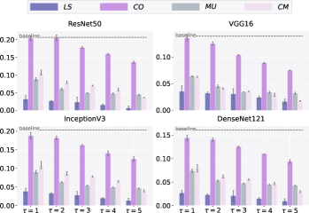
Figure 5: Gradient similarities between augmented surrogate and ST target CIFAR-10 models with error bars at each $\tau$.

Cutmix (CM) [82] also augments both images and labels by mixing samples. The difference is patches are cut and pasted among training samples. A mixed sample $\tilde{x}_{i,j}=\mathbf{M_{b}}\odot x_{i}+(\mathbf{1}-\mathbf{M_{b}})\odot x_{j}$ and its label $\tilde{y}_{i,j}$ are also obtained from two samples $(x_{i},y_{i}),(x_{j},y_{j})\in\mathbf{S}$, where $\mathbf{M_{b}}$ is a binary matrix with the same size of $x_{i}$ to indicate the location for cutting and pasting, $\mathbf{1}$ is a matrix filled with 1, and $b$ is drawn from $\operatorname{Beta}(1,1)$. $\tilde{y}_{i,j}$ is obtained similarly as MU. Similar to in MU, we use a probability parameter $\mathbf{p}$ to control the augmentation magnitude and train augmented models for CM with $\mathbf{p}\in[0.1,0.3,0.5,0.7,0.9]$.

Cutout (CO) [10] augments the dataset by masking out random regions of images with a size less than $M\times M$. In the real implementation, the mask-out region and its size for each image are not deterministic. A bigger $M$ value indicates it is more likely to mask out a bigger region. Hence, we utilize the value of $M$ only to regulate the extent of augmentation since it probabilistically governs the augmentation magnitude, similar to the role of $\mathbf{p}$ in MU and CM. We select $M\in[8,12,16,20,24]$ and $M\in[80,100,120,140,160]$ for CIFAR-10 and ImageNette, respectively.

Label smoothing (LS) [62] augments the dataset by replacing the hard labels $\mathcal{L}$ with soft continuous labels in probability distribution. Specifically, the probability of the ground-truth class is $1-p$, and the probability of other classes will be uniformly assigned to $p/(m-1)$, where $p\in[0,1)$ and $m$ denotes the number of classes. We train models for LS with $p\in[0.1,0.2,0.3,0,4,0.5]$.

These augmentations along with AT change data distributions in distinct manners. For a normal sample $(x,y)\sim\mathcal{D}$, AT associates input feature $x$ with ground-truth $y$ “inaccurately” under a noise $\delta$, while CO associates part of “right” $x$ with ground-truth $y$, thus they explicitly change the distribution on $\mathcal{P}_{\mathcal{X}}$. Contrarily, both MU and CM correlate parts of $x$ with $y$, causing shift in $\mathcal{P}_{\mathcal{X}\times\mathcal{Y}}$. Whereas LS relates the full $x$ to a “wrong” $y^{\prime}$, causing shift in $\mathcal{P}_{\mathcal{Y}}$. Intuitively, these augmentation methods will cause different impacts on the gradient $\nabla\ell_{\mathcal{F}}(x,y)$. As we select 5 augmentation magnitudes for each augmentation, we use a general parameter $\tau\in[1,2,3,4,5]$ to simplify the notations, e.g., $\tau=1$ means $\mathbf{p}=0.1$ for MU and $M=8$ for CO on CIFAR-10.

3.2 Data Augmentation Impairs Similarity

To verify Hypothesis 1, we explore how different data distribution shifts influence gradient similarity. For all the experiments, we train models with 3 different random seeds in each setting. Besides, multiple target models are considered to ensure generality. The results over 3 standard training (ST) models without augmentations are used as baselines.

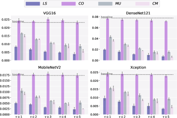
Figure 6: Gradient similarities between augmented surrogate and ST target ImageNette models with error bars at each $\tau$.

Figs. 5 and 6 depict the alignments towards multiple target models for CIFAR-10 and ImageNette. First, we observe that CO harms gradient similarity the least, but its effect varies across different datasets. Specifically, CO slightly degrades gradient similarity in CIFAR-10 while appearing comparable to baselines in ImageNette. The difference in training settings between the two datasets could be the reason for this gap; CIFAR-10 models are trained from scratch, while ImageNette models are obtained by fine-tuning well-trained ImageNet classifiers. These different outcomes suggest that simply removing some pixels is not enough to make the model forget what it has previously “seen”, since ImageNette is a 10-class subset of ImageNet. On the other hand, LS, MU, and CM degrade similarity largely over both datasets. Note that the similarity degradations of these augmentations are in line with their manipulations on $\mathcal{P}_{\mathcal{Y}}$, suggesting modifying the ground-truth $y$ during training results in more impacts on the direction of gradient $\nabla\ell_{\mathcal{F}}(x,y)$.

In summary, despite subtle differences, the results on both datasets support the hypothesis that data distribution shift impairs gradient similarity. Further, the distribution shift in $\mathcal{P}_{\mathcal{Y}}$ may have a greater negative impact on similarity than that in $\mathcal{P}_{\mathcal{X}}$.

3.3 Trade-off Under Data Augmentation

To figure out how these augmentations influence smoothness and transferability, we measure smoothness and the ASRs of AEs w.r.t. these augmented models. To save space, we merely report the $\tau=1,5$ cases for PGD attack in Tabs. II and III, as they represent the smallest and largest augmentation magnitudes. We report the $\tau=1,3,5$ cases for AutoAttack in Tab. XIII. Figs. 7 and 8 plots the smoothness for augmented models on two datasets.

First, LS exhibits a monotonous benefit on smoothness on both datasets due to its implicit effect on reducing the gradient norm during training [62]. However, the tables show that the ASRs of LS are always lower than those of ST, implying this benefit may not completely offset the negative effect of largely degraded similarity in LS. Additionally, there is no monotonicity in ASRs in LS, aligning with the always combating negative and positive effects. In contrast, other augmentations do not exhibit a consistent tendency for smoothness on both datasets. Specifically, in CIFAR-10, CM, MU, and CO mostly degrade the smoothness while the degradation is not strictly monotonous. The situation is even more chaotic in ImageNette, where the variances of smoothness are relatively large. However, the ASRs do reveal some patterns. For CM and MU, their ASRs degrade from $\tau=1$ to $\tau=5$, and the ASRs of CO are generally better than MU and CM. Notably, CO performs slightly better than ST under a few cases, especially when $\tau=1$. This agrees with the fact that CO has slightly better smoothness and less severely degraded similarity. Conclusively, the trade-off under data augmentations is quite complex, and no single augmentation can produce good surrogates.

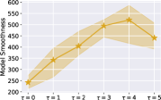
(a) MU

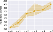
(b) CM

(c) CO

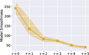
(d) LS

Figure 7: Average model smoothness of augmented models on CIFAR-10 with respective error bars at each $\tau$.

4 Investigating Gradient Regularization

At present, we recognize what may harm gradient similarity, but have no idea of how to generally improve it. Additionally, it is challenging to regulate similarity independently without affecting other factors, especially in black-box scenarios where target models are unknown. In contrast, the standalone model smoothness can be regulated and measured with the surrogate itself. Therefore, we will explore how gradient regularization, which is expected to improve smoothness without changing the data distribution, can be used to enhance surrogates.

4.1 Gradient Regularization Mechanisms

We first formally define gradient regularization and deliver the intuitions on why they are chosen. To sharpen the analysis, we introduce the notation $\theta$ to parameterize a neural network and reform $f(\cdot)$ as $f_{\theta}(\cdot)$ if needed. For concise illustrations, we sometimes abbreviate $l(f(x),y))$ as $l(f(x))$ in this section.

4.1.1 Regularization in the Input Space

Based on the implication that regularizing input space smoothness benefits transferability shown in Sec. 2.2, one should directly optimize the loss surface curvature. However, it is challenging to realize it since the computationally expensive second-order derivative is involved, i.e., $\nabla_{x}^{2}\ell(f_{\theta}(x))$. Fortunately, deep learning and optimization theory [16] allow us to use the first-order derivative to approximate it. We thus choose two well-known first-order gradient regularizations as follows:

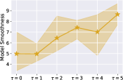
(a) MU

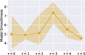
(b) CM

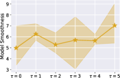
(c) CO

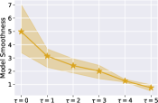
(d) LS

Figure 8: Average model smoothness of augmented models on ImageNette with respective error bars at each $\tau$.

Input gradient regularization (IR): IR directly add the Euclidean norm of gradient w.r.t. input to loss function as:

$$L_{ir}=\frac{1}{\left\|\mathbf{S}\right\|}\sum_{i=1}^{\left\|\mathbf{S}\right\|}[\ell(f(x_{i}))+\lambda_{ir}\|\nabla_{x}\ell(f(x_{i}))\|],$$

where $\lambda_{ir}$ controls the regularization magnitude. IR has been demonstrated improving the generalization and interpretability of DNNs [16, 51]. Here we show that IR can also improve transferability. Regularizing $\|\nabla_{x}\ell(f(x))\|_{2}$ leads to a smaller curvature $\sigma(\nabla_{x}^{2}\ell(x))$ because the spectral norm of a matrix is upper-bounded by the Frobenius norm, i.e., $\sigma(\nabla_{x}^{2}\ell(x))\leq\|\nabla_{x}^{2}\ell(x)\|_{F}\approx\|\nabla_{x}\ell(f(x))^{T}\nabla_{x}\ell(f(x))\|_{F}\leq\|\nabla_{x}\ell(f(x))\|^{2}$. Here we approximate the second-order derivative using the first-order derivative as suggested in [43, 28]. Consequently, smaller $\sigma(\nabla_{x}^{2}\ell(x))$ indicates better smoothness, thereby improving transferability.
Input Jacobian regularization (JR): JR regularizes gradients on the logits output of the network as:

$$L_{jr}=\frac{1}{\left\|\mathbf{S}\right\|}\sum_{i=1}^{\left\|\mathbf{S}\right\|}[\ell(f_{\theta}(x_{i})+\lambda_{jr}\|\nabla_{x}f_{\theta}(x_{i})\|_{F}].$$

JR has been also correlated with the generalization and robustness [28, 80, 4, 25, 64]. Since JR has a similar form with IR, it is reasonable to presume that they have a similar effect. Formally, we prove that when $\|\nabla_{x}f_{\theta}(x_{i})\|_{F}\rightarrow 0$, we have $\|\nabla_{x}\ell(f_{\theta}(x_{i}))\|\rightarrow 0$ using cross-entropy loss as an example (see Proposition 1). This implies that JR also has a positive effect on model smoothness.

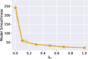
(a) IR

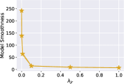
(b) JR

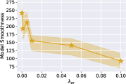
(c) ER

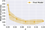
(d) SAM

Figure 9: Model smoothness of regularized models on CIFAR-10 with respective error bars at each $\tau$. The standard accuracy of these models ranges from 90.12% to 95.38%.

4.1.2 Regularization in the Weight Space

Recently, researchers paid attention to the gradient regularization on $\theta$, i.e., the parameters (weights) of the network. A recent study [11] proved that the gradient regularizing pressure on the weight space $\|\nabla_{\theta}f_{\theta}(x)\|_{F}$ can transfer to the input space $\|\nabla_{x}f_{\theta}(x)\|_{F}$. Consequently, regularizing gradients w.r.t. the weight space could also implicitly promote the smoothness in the input space. We next explore two representative weight gradient regularization methods as follows:
Explicit gradient regularization (ER): In ER, the Euclidean norm of gradient w.r.t. $\theta$ is added to the training loss $L_{er}$ to promote flatness as:

$$L_{er}(\theta)=L(\theta)+\frac{\lambda_{er}}{2}\|\nabla_{\theta}L(\theta)\|^{2},$$

where $L$ is the original objective function. Similar to IR and JR, we can directly apply the double-propagation technique to implement the regularization term, using the automatic differentiation framework provided by modern ML libraries like PyTorch [47]. ER has been empirically studied on improving generalization [3, 55, 20], while we investigate it from the transferability perspective.
Sharpness-aware minimization (SAM): SAM also seeks flat solution in the weight space. Specifically, it intends to minimize the original training loss and the worst-case sharpness $L_{sam}(\theta)=L(\theta)+[\max_{\|\boldsymbol{\hat{\theta}-\theta}\|_{2}\leq\rho}L(\hat{\theta})-L(\theta)]=\max_{\|\boldsymbol{\hat{\theta}-\theta}\|_{2}\leq\rho}L(\hat{\theta})$, where $\rho$ denotes the radius to search for the worst neighbor $\hat{\theta}$. As the exact worst neighbor is difficult to track, SAM uses the gradient of ascent direction neighbor for the update after twice approximations:

$$\nabla_{\theta}L_{sam}(\theta)\approx\nabla_{\theta}L(\theta+\rho\frac{\nabla_{\theta}L(\theta)}{||\nabla_{\theta}L(\theta)||}).$$

Recent researches establish SAM as a special kind of gradient normalization [85, 29], where $\rho$ represents the regularization magnitude. SAM has been extensively studied recently for its remarkable performance on generalization [18, 2, 6, 90, 70, 17, 1]. In this paper, for the first time, we substantiate that SAM also features outstanding superiority in boosting transferability.

4.2 Gradient Regularization Promotes Smoothness

We train multiple regularized models for each regularization and use coarse-grained parameter intervals [51, 18, 55] and restrict the largest regularized magnitude to avoid excessive regularization such that the accuracy of these models are above 90%. This allows for a fair comparison of each regularization method in an acceptable accuracy range. We choose 5 parameters in each interval through random grad and binary choices (See Tab. XI).

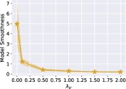
(a) IR

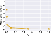
(b) JR

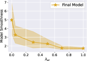
(c) ER

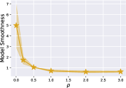
(d) SAM

Figure 10: Model smoothness of regularized models on ImageNette with respective error bars at each $\tau$. The standard accuracy of these models ranges from 90.62% to 96.91%.

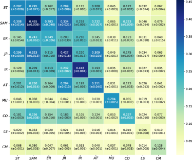
(a) ResNet18 trained over CIFAR-10

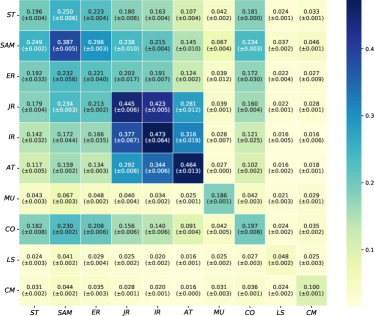
(b) ResNet50 trained over ImageNette

Figure 11: Intra-architecture gradient similarity between different mechanisms. Each cell reports the average result of 3 unique source-target pairs while all pair of models are trained with different random seeds, hence each matrix is asymmetric.

Figs. 9 and 10 depict the model smoothness. We can observe gradient regularizations generally result in smoother models (i.e., smaller values) than the baseline where the regularization magnitude is 0 (ST), and large magnitudes correspond to better smoothness. Moreover, input gradient regularizations yield much better smoothness than weight gradient regularizations, particularly on CIFAR-10. This indicates that the transfer effect from weight space to input space suggested in [11] does exist, yet is somewhat marginal and cannot outperform direct regularizations in input space.

4.3 Trade-off Under Gradient Regularization

One might presume that input gradient regularization (JR, IR) should clearly outperform weight gradient regularization (SAM, ER) in terms of transferability, which agrees with the conclusion that less complexity should exhibit better transferability in Demontis et al. [9], given that smoothness is positively correlated to the model complexity (as analyzed in Sec. 6, Q3). However, our experimental results counter this:

• In Tab. II (CIFAR-10), the fact is that SAM is generally better than IR (11 out of 12 cases for untargeted attacks, 12 out of 12 for targeted), and generally better than JR (11 out of 12 cases for untargeted, 7 out of 12 for targeted).

• In Tab. III (ImageNette), the fact is that SAM is generally worse than IR (11 out of 12 cases for untargeted 10 out of 12 for targeted), and consistently worse than JR (12 out of 12 cases for both targeted and untargeted).

Therefore, these inconsistent results do not allow us to conclude that better smoothness always leads to better or worse transferability. This finding not only weakens the conclusion in Demontis et al. [9], but also suggests an overall examination of these training mechanisms for superior surrogates, as they may weigh differently on similarity.

5 Boosting Transferability with Surrogates

Although we have concluded that gradient regularization can generally improve smoothness, the intangible nature of gradient similarity towards unknown target models still makes it difficult to guide us in obtaining better surrogates. We thus propose a general solution that can simultaneously improve smoothness and similarity, under a strict black-box scenario where target models are inaccessible. Our strategy involves first examining the pros and cons of various training mechanisms w.r.t. smoothness and similarity, and then combining their strengths to train better surrogates.

While gradient similarity cannot be directly measured when target models are unknown, one can assess the similarity between all the training mechanisms under the intra-architecture case instead. This helps to draw general conclusions that can be extended to the cross-architecture case as the angles between gradient directions follow the triangle inequality. Therefore, we measure the similarity between the surrogates we obtained thus far, reported in Fig. 11. Tab. VII in Sec. 6, Q2 can support the consistency posteriorly with observations in the cross-architecture case. As a result, we obtain surrogates featuring both superior smoothness and similarity on average, and extensive experiments demonstrate their superiority in transferability.

5.1 A General Route for Better Surrogates

We first elaborate on some general observations about gradient regularization mechanisms as follows:

Table IV: Untargeted and targeted transfer ASRs when incorporating AE generation strategies under the different $L_{\infty}$ budgets on CIFAR-10. Corresponding results are different from those of Tab. II due to different randomization. In %.

	Untargeted								Targeted
	4/255				8/255				4/255				8/255
	Res-50	VGG16	Inc-V3	Dense-121	Res-50	VGG16	Inc-V3	Dense-121	Res-50	VGG16	Inc-V3	Dense-121	Res-50	VGG16	Inc-V3	Dense-121
ST	55.0±2.4	43.3±2.1	54.9±2.5	71.7±1.2	79.6±2.6	71.3±3.2	80.2±3.8	93.1±1.3	19.0±1.2	13.2±1.0	21.1±1.5	36.4±1.8	41.1±4.7	34.3±3.7	45.8±4.2	70.8±4.6
SAM	76.8±4.7	65.0±5.3	74.9±0.6	87.4±1.2	97.5±1.2	94.3±2.2	97.0±0.2	99.5±0.1	37.1±6.4	27.2±5.0	38.5±2.0	55.8±3.7	77.2±9.2	68.3±8.4	78.4±2.7	93.4±0.9
SAM&JR	81.2±0.7	70.2±0.7	79.4±0.6	91.3±0.1	98.7±0.3	96.6±0.1	98.3±0.0	99.8±0.0	43.6±2.1	32.9±1.2	45.3±2.1	64.5±0.9	85.4±1.4	77.2±9.2	86.8±1.9	97.2±0.3
ST+MI	58.4±2.6	45.0±2.9	58.7±4.0	76.7±2.3	82.9±3.1	75.6±4.1	83.5±3.6	94.6±1.2	22.4±1.8	15.4±1.9	25.6±2.8	46.0±3.9	44.8±4.1	40.2±5.9	50.4±6.3	76.1±4.5
SAM+MI	82.3±3.9	69.6±5.3	80.5±0.1	91.7±1.5	98.1±0.9	95.5±1.9	97.8±0.1	99.7±0.1	46.7±7.0	33.2±5.7	49.0±1.1	69.6±3.8	84.0±6.9	76.9±5.8	84.8±1.2	96.4±0.9
SAM&JR+MI	85.0±0.4	73.8±0.5	83.3±0.5	93.6±0.1	98.9±0.2	97.2±0.2	98.7±0.1	99.8±0.1	52.4±2.0	38.4±1.5	54.0±1.7	74.5±0.4	89.6±1.6	82.9±1.5	90.6±2.1	98.3±0.3
ST+DIM	70.2±3.8	59.2±2.7	69.2±3.5	83.6±3.1	91.9±2.2	88.3±2.8	91.7±2.2	97.2±1.3	33.6±4.8	25.7±3.2	36.6±4.2	54.9±6.3	65.4±6.3	62.0±6.2	69.9±5.3	87.5±5.3
SAM+DIM	84.4±2.6	74.7±2.7	82.2±1.8	91.8±2.2	98.9±0.4	97.7±0.7	99.1±0.8	99.7±0.2	50.4±4.6	38.9±3.2	51.3±4.2	67.8±5.8	89.3±3.5	84.2±2.2	89.6±3.0	96.8±1.9
SAM&JR+DIM	83.6±1.6	74.8±1.0	81.8±1.4	92.1±0.6	99.2±0.2	98.2±0.3	99.0±0.1	99.8±0.1	51.6±3.9	40.7±2.4	52.7±2.9	70.2±2.0	91.5±2.9	86.9±2.8	91.8±2.6	98.1±0.8

• Input regularizations stably yield the best smoothness. Figs. 9 and 10 show that IR and JR yield superior smoothness and their variances are small. This does not hold for other smoothness-benefiting mechanisms like SAM, ER. Further, Fig. 11 suggests that IR, JR, and AT align superiorly well with each other, this could be attributed to the fact that they all have a direct penalty effect on the input space, as analyzed in Secs. 2.3 and 4.1.1.

• SAM yields the best gradient alignments when input regularizations are not involved. Fig. 11 shows that SAM exclusively exhibits better alignment towards every mechanism than ST. However, other mechanisms do not exhibit this advantage. Furthermore, if we exclude the diagonal elements, we can find SAM yields the best gradient similarity in each row and column except for the cases of IR, JR, and AT. This suggests that SAM has an underlying benefit on gradient similarity, which all the other mechanisms do not hold. We defer the detailed analysis on this to Sec. 6, Q7.

• No single mechanism can dominate both datasets. From Tabs. II and III, we observe that SAM yields the best ASRs on average on CIFAR-10. However, it generally performs worse than IR and JR on ImageNette. ER, on the other hand, consistently performs the worst on two datasets. Apparently, there is no one mechanism that can adequately outperform the others on both datasets.

The above observations inspire us that SAM and input regularization are highly complementary, and a straightforward solution to reach a better trade-off between model smoothness and gradient similarity is combining SAM with input regularization, namely SAM&IR or SAM&JR. In other words, we believe SAM&IR and SAM&JR will bring significant improvement in transferability. To validate this hypothesis, we conduct experiments on both CIFAR-10 and ImageNette and report the results on Tabs. II and III for comparison. We can see that SAM&JR and SAM&IR generally perform the best in both datasets. Notably, we do not limit the route of constructing better surrogates to SAM&IR or SAM&JR, and there may exist other effective combinations or approaches as long as the trade-off is well reconciled.

5.2 Incorporating Surrogate-independent Methods

We show that the surrogates obtained from our methods (e.g., SAM and SAM&JR) can be integrated with surrogate-independent methods to further improve transferability.

5.2.1 Incorporating AE generation strategies

Exploiting the generation process of AEs is a popular approach to improve transferability. The most representative methods include momentum iterative (MI) [12] and diversity iterative (DI) [76], and DI is frequently combined with MI and serves as a stronger baseline—diversity iterative with momentum (DIM). Generally, these designs are interpreted as constructing adversarial examples that are less likely to fall into a poor local optimum of the given surrogate. Thus they adjust the update direction with momentum to escape it or apply multiple transformations on inputs to mimic an averagely flat landscape. We conduct experiments to verify that obtaining a better surrogate, which features less and wider local optima (analyzed in Sec. 6, Q3) and general adversarial direction, can further enhance these designs by promoting a larger lower bound.

In Tab. IV, the transfer ASRs under different generation strategies (PGD, MI, and DIM) show that using better surrogates can always significantly boost transferability. This suggests that the optima found in ST are inherently poorer than those in SAM and SAM&JR. Besides, without MI or DIM, SAM&JR using standard PGD alone already outperforms ST+MI and ST+DMI, implying that the lower bound of transferability in a better surrogate is sufficiently high, and even surpasses the upper bound in poor models.

Table V: Transfer ASRs of AEs crafted against single and LGV ensemble surrogates under the different $L_{\infty}$ budgets on CIFAR-10. Single surrogates without fine-tuning are used for baselines and compared with LGV ensembles. We highlight the best ASRs in bold and those lower than baselines in red for each comparison. In %.

	Untargeted								Targeted
	4/255				8/255				4/255				8/255
	Res-50	VGG16	Inc-V3	Dense-121	Res-50	VGG16	Inc-V3	Dense-121	Res-50	VGG16	Inc-V3	Dense-121	Res-50	VGG16	Inc-V3	Dense-121
ST	55.0±2.4	43.3±2.1	54.9±2.5	71.7±1.2	79.6±2.6	71.3±3.2	80.2±3.8	93.1±1.3	19.0±1.2	13.2±1.0	21.1±1.5	36.4±1.8	41.1±4.7	34.3±3.7	45.8±4.2	70.8±4.6
ST+$\rm{LGV_{\text{SGD}}}$	70.7±2.2	57.1±1.1	70.1±0.9	87.1±0.6	94.0±2.0	89.1±2.5	94.3±1.8	99.3±0.2	29.3±2.0	20.4±1.3	32.8±2.1	53.4±2.1	65.6±4.2	56.8±3.2	71.3±2.5	92.0±1.2
ST+$\rm{LGV}_{\textit{SAM}}$	79.5±0.8	66.8±1.1	79.8±1.0	92.3±0.2	98.6±0.2	96.0±0.5	98.7±0.2	99.9±0.0	39.4±1.0	27.7±0.5	44.4±1.7	65.7±0.9	82.5±1.7	74.2±1.0	87.4±0.8	97.8±0.2
ST+$\rm{LGV}_{\textit{SAM}\&\textit{JR}}$	82.0±1.5	69.5±1.7	81.3±1.3	93.4±0.3	99.1±0.3	97.1±0.7	99.0±0.2	99.9±0.0	42.9±2.6	30.3±1.5	46.7±1.4	68.1±1.0	87.1±3.5	79.1±3.4	90.2±1.7	98.5±0.3
SAM	76.8±4.7	65.0±5.3	74.9±0.6	87.4±1.2	97.5±1.2	94.3±2.2	97.0±0.2	99.5±0.1	37.1±6.4	27.2±5.0	38.5±2.0	55.8±3.7	77.2±9.2	68.3±8.4	78.4±2.7	93.4±0.9
SAM+$\rm{LGV_{\text{SGD}}}$	70.8±6.1	57.2±6.5	69.2±0.7	84.2±0.7	93.1±3.9	87.6±5.3	93.2±1.4	98.6±0.3	26.7±1.9	18.7±0.1	31.5±2.2	51.3±2.6	63.6±14.1	53.6±11.8	66.4±5.4	87.6±2.2
SAM+$\rm{LGV}_{\textit{SAM}}$	81.5±4.0	69.5±4.8	79.8±1.3	91.6±1.3	98.9±0.7	96.9±1.3	98.7±0.1	99.9±0.0	42.1±7.3	30.5±5.5	44.3±1.6	63.4±1.9	86.2±6.7	78.4±6.6	87.9±1.1	97.5±0.4
SAM+$\rm{LGV}_{\textit{SAM}\&\textit{JR}}$	82.7±4.2	71.2±5.1	80.9±0.6	92.1±1.2	99.1±0.6	97.4±1.3	99.0±0.3	99.9±0.0	44.7±7.7	32.6±5.9	46.6±0.6	65.6±1.7	87.6±6.9	79.8±7.1	89.1±2.0	97.9±0.5
SAM&JR	81.2±0.7	70.2±0.7	79.4±0.6	91.3±0.1	98.7±0.3	96.6±0.1	98.3±0.0	99.8±0.0	43.6±2.1	32.9±1.2	45.3±2.1	64.5±0.9	85.4±1.4	77.2±2.1	86.8±1.9	97.2±0.3
SAM&JR+$\rm{LGV_{\text{SGD}}}$	73.8±1.8	61.1±1.6	73.1±1.8	88.3±0.5	95.8±1.1	90.9±1.9	95.6±1.1	99.4±0.1	35.6±2.9	25.1±2.4	39.0±2.7	60.2±1.7	70.5±5.0	61.1±5.9	74.5±5.7	93.6±1.5
SAM&JR+$\rm{LGV}_{\textit{SAM}}$	82.5±0.7	71.2±1.0	81.0±0.4	93.0±0.2	99.1±0.1	97.4±0.2	98.9±0.1	99.9±0.1	44.0±1.5	32.2±1.1	46.8±1.4	67.6±0.8	87.6±1.2	80.2±1.7	89.7±1.2	98.4±0.1
SAM&JR+$\rm{LGV}_{\textit{SAM}\&\textit{JR}}$	83.8±0.8	72.9±1.2	82.5±0.9	93.7±0.1	99.3±0.1	97.8±0.3	99.3±0.1	99.9±0.0	46.9±1.4	34.8±1.2	49.5±1.0	70.0±0.5	90.0±0.9	83.2±0.7	91.8±0.7	98.8±0.1

5.2.2 Incorporating ensemble strategies

Using multiple surrogates is widely believed to update adversarial examples in a more general direction that benefits transferability. Recently, [23] proposed constructing the ensemble from a large geometric vicinity (LGV), i.e., first fine-tuning a normally trained model with a high constant learning rate to obtain a set of intermediate models that belongs to a large vicinity, then optimizing AEs iteratively against all these models. We conduct experiments to verify whether SAM and SAM&JR can further enhance this ensemble and analyze how their intrinsic mechanisms correlate with LGV. Specifically, we fine-tune models well-trained with SGD, SAM, and SAM&JR on CIFAR-10 using SGD, SAM, and SAM&JR with a constant learning rate of 0.05.

In Tab. V, the transfer results show that LGV with SAM, SAM&JR can always yield superior ASRs than standard SGD, indicating that the underlying property of SAM and JR allows them to find solutions that benefit transferability. More intriguingly, fine-tuning models obtained by SAM and SAM&JR with SGD always brings non-negligible negative impacts on transferability. These suggest solutions well-trained with SAM and SAM&JR lie in the basin of attractions featuring better transferability, and a relatively high constant learning rate with SGD will arbitrarily minimize the training loss while leaving the basin of attractions. Note that a relatively high constant learning rate is necessary for a large vicinity [23], thus we can infer that a large vicinity may not be a determining factor for transferability since a single surrogate can outperform an ensemble of poor surrogates (see SAM&JR and ST+$\rm{LGV_{\text{SGD}}}$). Instead, a dense subspace whose geometry is intrinsically connected to transferability is more desirable.

5.2.3 Incorporating other strategies

We take AE generation and ensemble strategies, which are the most well-explored methods, to exemplify the universality of better surrogates. We are aware of other factors that could also contribute to transferability, such as loss object modification [86], architecture selection [72], $l_{2}$-norm consideration [42], unrestricted generation [26, 87], patch-based AEs [27]. We leave it to our future work to investigate whether they can be mildly integrated with our design.

6 Analyses and Discussions

Q1: Does the trade-off between smoothness and similarity really “significantly indicate” transferability w.r.t. surrogates? Our theoretical analysis and experimental validation have demonstrated the significant role of smoothness and similarity in regulating transferability among surrogate-side factors. To investigate whether their impact on transferability is significant, we calculate the respective Pearson correlation coefficients between the surrogate-related factors and ASR and run ordinary least squares (OLS) regressions to measure their joint effect on ASR. Tab. VI reports the results under each fixed target model and adversarial budget, which indicates that both smoothness and similarity are highly correlated to ASR, with a clear superiority over other factors. Besides, the joint effect of smoothness and similarity ($R^{2}_{1}$) is significant in each case and very close to that of the 4 factors combined ($R^{2}_{2}$). Further, it does not exhibit a strong correlation with $\epsilon$ under each target model, indicating the joint effect is indeed strong and robust.

Interestingly, we can observe that as $\epsilon$ increases, the relevance w.r.t. smoothness alone increases, and the relevance w.r.t. similarity alone decreases. This agrees with the intuition: smoothness depicts the gradient invariance around origin, while similarity captures the alignment of two gradients in different directions. As $\epsilon$ approaches 0, smoothness becomes less important for the gradient may not vary too much in a small region, and the legitimate direction becomes more crucial since there is limited scope for success. As $\epsilon$ gets bigger, the alignment at the origin requires better smoothness to be further propagated into a bigger region. These suggest an adaptive similarity-smoothness trade-off surrogate could be preferable given different $\epsilon$.

Table VI: The Pearson correlation coefficients ($r$) between ASR and accuracy ($Acc$), fooling probability ($FP$), model smoothness ($MS$), and gradient similarity ($GS$). For the coefficient of determination ($R^{2}$) in OLS, $R_{1}^{2}$ depicts the joint effect of $MS$ and $GS$ on ASR and $R_{2}^{2}$ depicts the joint effect of these 4 factors.

CIFAR-10
	ResNet50			VGG16			InceptionV3			DenseNet121
	$\frac{\textrm{4}}{\textrm{255}}$	$\frac{\textrm{8}}{\textrm{255}}$	$\frac{\textrm{16}}{\textrm{255}}$	$\frac{\textrm{4}}{\textrm{255}}$	$\frac{\textrm{8}}{\textrm{255}}$	$\frac{\textrm{16}}{\textrm{255}}$	$\frac{\textrm{4}}{\textrm{255}}$	$\frac{\textrm{8}}{\textrm{255}}$	$\frac{\textrm{16}}{\textrm{255}}$	$\frac{\textrm{4}}{\textrm{255}}$	$\frac{\textrm{8}}{\textrm{255}}$	$\frac{\textrm{16}}{\textrm{255}}$
$r(Acc,ASR)$	0.121	-0.049	-0.255	0.032	-0.095	-0.259	0.211	0.028	-0.187	0.286	0.130	-0.107
$r(FP,ASR)$	0.118	0.106	0.055	0.197	0.164	0.098	0.105	0.091	0.040	0.051	0.008	-0.033
$r(MS,ASR)$	0.540	0.662	0.753	0.614	0.700	0.774	0.478	0.630	0.732	0.418	0.581	0.701
$r(GS,ASR)$	0.912	0.837	0.759	0.924	0.878	0.816	0.864	0.743	0.653	0.875	0.710	0.585
$R^{2}_{1}$	0.909	0.885	0.879	0.917	0.906	0.893	0.870	0.827	0.838	0.880	0.773	0.765
$R^{2}_{2}$	0.943	0.892	0.894	0.931	0.907	0.913	0.911	0.843	0.852	0.926	0.823	0.799
ImageNette
	VGG16			DenseNet121			MobileNetV2			Xception
	$\frac{\textrm{4}}{\textrm{255}}$	$\frac{\textrm{8}}{\textrm{255}}$	$\frac{\textrm{16}}{\textrm{255}}$	$\frac{\textrm{4}}{\textrm{255}}$	$\frac{\textrm{8}}{\textrm{255}}$	$\frac{\textrm{16}}{\textrm{255}}$	$\frac{\textrm{4}}{\textrm{255}}$	$\frac{\textrm{8}}{\textrm{255}}$	$\frac{\textrm{16}}{\textrm{255}}$	$\frac{\textrm{4}}{\textrm{255}}$	$\frac{\textrm{8}}{\textrm{255}}$	$\frac{\textrm{16}}{\textrm{255}}$
$r(Acc,ASR)$	0.218	0.128	-0.047	0.133	0.023	-0.165	0.093	-0.014	-0.196	0.072	-0.028	-0.177
$r(FP,ASR)$	0.121	0.120	-0.055	0.146	0.117	-0.081	-0.034	0.003	-0.151	0.062	-0.012	-0.156
$r(MS,ASR)$	0.410	0.472	0.516	0.458	0.503	0.492	0.495	0.576	0.625	0.499	0.571	0.624
$r(GS,ASR)$	0.864	0.829	0.764	0.859	0.855	0.853	0.789	0.766	0.780	0.753	0.722	0.721
$R^{2}_{1}$	0.854	0.841	0.780	0.821	0.843	0.832	0.715	0.742	0.804	0.688	0.704	0.752
$R^{2}_{2}$	0.871	0.847	0.798	0.854	0.850	0.867	0.750	0.752	0.833	0.712	0.707	0.781

Q2: What if the target model is not trained on $\mathcal{D}$? So far, we presume the target models are trained within the normal data distribution $\mathcal{D}$ to lay out our analysis and conclusions, which is also set by default in Demontis et al. [9]. To verify the generality of the obtained conclusion, we deliver the results here when the data distribution restrictions of target model $\mathcal{G}$ is relaxed. First, we generalize Hypothesis 1 as:

Hypothesis 2 ($\mathcal{D}$-surrogate aligns general target models better than $\mathcal{D}^{\prime}$-surrogate).

Suppose surrogates $\mathcal{F}_{\mathcal{D}}$ and $\mathcal{F}_{\mathcal{D}^{\prime}}$ are trained on $\mathcal{D}$ and $\mathcal{D}^{\prime}$ respectively. Denote the data distribution of target model $\mathcal{G}_{\mathcal{D}_{t}}$ as $\mathcal{D}_{t}\in\mathcal{P}_{\mathcal{X}\times\mathcal{Y}}$. They share a joint training loss $\ell$. Then $\mathbb{E}_{\mathcal{D}_{t}\sim P_{\mathcal{X}\times\mathcal{Y}}}[\tilde{\mathcal{S}}_{\mathcal{D}}\left(\ell_{\mathcal{F}_{\mathcal{D}^{\prime}}},\ell_{\mathcal{G}_{\mathcal{D}_{t}}}\right)-\tilde{\mathcal{S}}\left(\ell_{\mathcal{F}_{\mathcal{D}}},\ell_{\mathcal{G}_{\mathcal{D}_{t}}}\right)]<0$ generally holds.

This hypothesis considers a more practical case that the adversary has no knowledge of $\mathcal{D}_{t}$, and tries to attack $\mathcal{G}_{\mathcal{D}_{t}}$ with AEs constructed on normal samples $(x,y)\in\mathcal{D}$. The adversary hopes its surrogate aligns well with any $\mathcal{G}_{\mathcal{D}_{t}}$ regardless of what $\mathcal{D}_{t}$ is. We show that $\mathcal{D}$-surrogate $\mathcal{F}_{\mathcal{D}}$ is still better than $\mathcal{D}^{\prime}$-surrogate $\mathcal{F}_{\mathcal{D}}^{\prime}$ based on the expectation over various $\mathcal{D}_{t}$.

Tab. VII reports the general surrogate-target gradient similarities. It’s obvious that $\mathcal{D}^{\prime}$ surrogates (above AT) generally worsen the gradient alignments as their increment scores are all negative, except for AT with a small budget $\epsilon=0.01$. Conversely, the scores of $\mathcal{D}$ surrogates (below AT) are all non-negative and most of them improve the general alignment. Note that when $\mathcal{D}^{\prime}$ happens to be $\mathcal{D}_{t}$, the gradient similarity between $\mathcal{F}_{\mathcal{D}}^{\prime}$ and $\mathcal{G}_{\mathcal{D}_{t}}$ is high, especially for CM and MU. However, these surrogates lower the similarity towards all other targets. In general, they are not good surrogates since $\mathcal{D}_{t}$ is unknown to the adversary.

The same observations apply to the transfer ASRs. Tab. VIII reports the transfer ASRs against various $\mathcal{G}_{\mathcal{D}_{t}}$ that are not trained on $\mathcal{D}$. Even when surrogates have the same training mechanisms as the corresponding target models, the best surrogate is still either SAM&IR or SAM&JR,  regardless of what $\mathcal{D}_{t}$ is. This finding is in line with the results in Tab. II.

Table VII: Cross-architecture gradient similarity between surrogate-target pairs (ResNet18-VGG16) on CIFAR-10. The first row reports the results of ST surrogate, below which report the difference to ST. The last column rates the score of the surrogates based on the general alignment toward multiple targets. (Accumulate +1 for positive, -1 for negative values.)

		ST	CO	CM	MU	LS	AT	Increment Score
$\,\,\mathcal{D}\,\,$	ST	0.141	0.135	0.056	0.038	0.014	0.131	0
$\,\,\mathcal{D^{\prime}}\,\,$	CO	-0.038	+0.005	-0.001	+0.004	-0.001	-0.041	-2
	CM	-0.105	-0.084	+0.008	-0.021	-0.006	-0.098	-4
	MU	-0.106	-0.092	-0.030	+0.122	-0.003	-0.102	-4
	LS	-0.094	-0.098	-0.033	-0.013	+0.008	-0.090	-4
	AT	-0.002	-0.005	-0.013	+0.001	+0.001	+0.047	0
$\,\,\mathcal{D}\,\,$	IR	-0.002	-0.014	-0.020	+0.008	+0.007	+0.043	0
	JR	+0.044	+0.028	+0.004	+0.012	+0.004	+0.072	+6
	ER	+0.012	+0.006	-0.013	+0.011	+0.005	+0.031	+4
	SAM	+0.055	+0.057	+0.007	+0.029	+0.006	+0.058	+6
	SAM&IR	+0.012	+0.001	-0.021	+0.016	+0.010	+0.065	+4
	SAM&JR	+0.078	+0.072	+0.008	+0.035	+0.010	+0.093	+6

Q3: What is the relationship between model smoothness and model complexity? Model complexity has been investigated in Demontis et al. [9] to figure out whether it correlates with transferability, which is defined as the variability of the loss landscape, deriving from the number of local optima of the surrogates. Here we correlate the number of local optima with model smoothness. It is obvious that a high-complexity model featuring multiple local optima will cause a larger variance to the loss landscape of AE optimization. Formally, for a feature $x$, the fewer optima in its $\epsilon$-neighbor, the smaller the variance would be. Thus, supposing the loss function used to optimize adversarial points is continuously differentiable, by promoting the smoothness, we can expect fewer optima in the finite $\epsilon$-neighbor space since all the local optima are wider. Consequently, model smoothness negatively correlates with model complexity, i.e., a smoother model indicates lower complexity.

Table VIII: Transfer ASRs of AEs crafted from various ResNet18 surrogates against VGG16 target models trained with AT and augmentations on CIFAR-10. $\bigstar$ denotes that surrogates have the same training methods as the corresponding target models. ‘T’ represents ‘Targeted’ attack and ‘U’ represents ‘Untargeted’ attack.

	AT, $\epsilon=0.01$		AT, $\epsilon=0.05$		CM		CO		LS		MU
	T	U	T	U	T	U	T	U	T	U	T	U
ST	20.18	51.33	4.83	22.49	42.42	79.49	38.80	76.33	34.62	72.34	37.46	69.25
$\bigstar$	43.01	76.96	35.54	69.56	14.20	54.57	32.91	79.11	11.90	46.66	15.81	54.43
IR	60.08	91.23	31.84	73.98	59.80	91.82	60.78	92.14	63.20	93.52	60.79	90.06
JR	57.24	83.54	14.57	41.77	73.44	92.47	74.77	93.03	72.27	92.30	68.34	86.90
ER	32.61	77.14	9.55	40.41	41.94	86.92	43.04	87.39	44.51	87.77	42.12	82.66
SAM	40.35	79.31	8.41	35.05	75.34	96.59	67.72	94.84	62.68	93.57	65.37	90.43
SAM&IR	71.88	94.01	48.38	80.88	70.81	93.75	73.05	94.31	74.02	95.47	70.81	92.68
SAM&JR	58.81	89.23	15.11	47.11	83.56	97.57	80.19	97.02	77.95	96.92	75.06	94.49

Q4: Does a smaller model generalization gap imply higher adversarial transferability? It is natural to raise this question as the idea of adversarial transferability in a way resembles the concept of model generalization. The former captures the effectiveness of AEs against unseen models, while the latter evaluates the model’s ability to adapt properly to previously unseen data. A concurrent work [68] attempts to show the positive relationship between model generalization and adversarial transferability, by applying a spectral normalization method constraining the $L_{2}$-operator norm of the surrogate’s weight matrix to empirically demonstrate the increase of both transferability and generalization.

Nevertheless, we emphasize that we cannot over-generalize the alignment between generalization and transferability. It is easy to find some cases that boost generalization yet degrades transferability (e.g., through damaging similarity). For example, the results in Tabs. II, III, XIII and X have shown augmentations that boost generalization could sacrifice transferability. More typically, the strong data augmentations that yield the smallest generalization gaps (see Tab. XII) perform the worst in transfer attacks. In fact, the product of spectral norm of model’s layer-wise weight matrices is a loose upper bound of $\|\nabla_{x}f_{\theta}(x)\|_{2}$ [52, 80]. When $\|\nabla_{x}f_{\theta}(x)\|_{2}\rightarrow 0$, we have $\|\nabla_{x}f_{\theta}(x)\|_{F}\rightarrow 0$. Utilizing Proposition 1, we also have $\|\nabla_{x}\ell(f_{\theta}(x),y)\|\rightarrow 0$. This suggests that spectral normalization actually benefits transferability by promoting smoothness.

Q5: What is restraining the adversarial transferability of ViT? Recently, ViT [15] receives notable attention for its outstanding performance on various tasks. Meanwhile, some works [54, 41] have demonstrated that ViT models exhibit lower adversarial transferability than CNNs when used as surrogates, and a recent work [46] argues that this is because the current attacks are not strong enough to fully exploit the transferability potential of ViT. Complementarily, we provide a different viewpoint that the transferability of ViT may have been restrained by its own training paradigm. ViT is known to have poor trainability [7, 6], and thus generally requires large-scale pre-training and fine-tuning with strong data augmentations. This training paradigm is used by default since its appearance. However, as we discussed in this paper, changing the data distribution could have negative impacts on similarity. Using data augmentation is plausible for accuracy performance, yet not ideal for transfer attacks.

Table IX: Untargeted transfer ASRs of AEs crafted against ViT ImageNet surrogates on target models. In %.

Source	Acc	Normally Trained				Adversarially Trained
		Res101	Dense121	VGG16	IncV3	IncV3 ${}_{\textit{AT}}$	IncResV3${}_{\textit{AT}}$
ViT-B/16	84.5	23.8	37.6	50.0	45.9	48.6	27.6
ViT-B/16-SAM	80.2	48.4	69.9	75.2	70.2	59.5	40.5
ViT-B/32	80.7	19.6	35.7	50.0	49.1	51.9	29.7
ViT-B/32-SAM	73.7	34.0	55.8	68.9	64.3	63.1	43.9
ViT-B/16+DIM	84.5	60.7	75.3	79.9	80.0	61.4	43.8
ViT-B/16-SAM+DIM	80.2	81.6	95.6	93.9	94.6	82.4	79.9
ViT-B/32+DIM	80.7	48.4	66.4	75.2	81.6	68.6	54.4
ViT-B/32-SAM+DIM	73.7	48.9	78.1	78.4	82.5	79.3	72.3

To validate this standpoint, we show that with a different training method such as SAM, the transferability of ViT can be significantly improved. Our experiments are conducted on well-trained ImageNet classifiers, all publicly available from PyTorch image model library timm [71]. We consider standard ViT surrogates ViT-B/16 and ViT-B/32, which are both first pre-trained on a large-scale dataset and then fine-tuned on ImageNet using a combination of MU and RandAugment [8]. In contrast, their SAM versions ViT-B/16-SAM and ViT-B/32-SAM are merely trained from scratch. We use both normally and adversarially trained CNN classifiers as target models. We craft AEs on these 4 surrogates using both standard PGD and DIM under $\epsilon=16/255$ on the ImageNet-compatible dataset as in [49]. The accuracy of these surrogates (referring to [71]) and ASRs are reported in Tab. IX. The results indicate that standard ViT models have much weaker transferability than their SAM versions, despite the fact that they have higher accuracy.

Q6: Will the transferability benefit of better surrogate in “lab” generalize to “real-world” environment? Recently, Mao et al. [42] suggests that many conclusions about adversarial transferability done in the simplistic controlled “lab” environments may not hold in the real world. We thus conduct experiments to verify the generality of our conclusions using AEs crafted against our ImageNette surrogates.

Specifically, aligning with Mao et al. [42], we conduct transfer attacks on three commercial MLaaS platforms—AWS Rekognition, Alibaba Cloud, and Baidu Cloud, using their code, and report the results in Tab. X. The results are generally consistent with that in Tab. III. Particularly, we highlight here that our experimental results on MLaaS platforms contradict the observation in Mao et al. [42] that “adversarial training and data augmentation do not show strong correlations to the transfer attack”. Tab. X indicates that strong data augmentations like CM and MU generally exhibit lower ASRs than ST for both targeted and untargeted attacks. In addition, we can observe that “little robustness” (see AT, $\epsilon=1$) improves transferability while large adversarial magnitude (see AT, $\epsilon=5$) degrades it.

Q7: How does SAM yield superior alignment towards every training solution? Given its superior performance on transferability and gradient alignment, it is natural to wonder why SAM exhibits this property. Recent works [22, 33] empirically demonstrate that attacking an ensemble of models in the distribution obtained via Bayesian learning substantially improves the transferability.

Table X: Transfer ASRs under the different $L_{\infty}$ budgets on 3 MLaaS platforms using AEs reported in Tab. III.

	Untargeted						Targeted
	AWS		Baidu		Aliyun		AWS		Baidu		Aliyun
Model	$\frac{\textrm{8}}{\textrm{255}}$	$\frac{\textrm{16}}{\textrm{255}}$	$\frac{\textrm{8}}{\textrm{255}}$	$\frac{\textrm{16}}{\textrm{255}}$	$\frac{\textrm{8}}{\textrm{255}}$	$\frac{\textrm{16}}{\textrm{255}}$	$\frac{\textrm{8}}{\textrm{255}}$	$\frac{\textrm{16}}{\textrm{255}}$	$\frac{\textrm{8}}{\textrm{255}}$	$\frac{\textrm{16}}{\textrm{255}}$	$\frac{\textrm{8}}{\textrm{255}}$	$\frac{\textrm{16}}{\textrm{255}}$
ST	9.4	13.4	30.0	53.8	18.6	52.2	23.0	23.8	11.6	16.6	2.6	6.4
MU	8.6	10.8	20.4	39.6	12.4	33.8	20.4	23.8	9.6	15.0	1.4	2.8
CM	8.0	10.8	19.4	35.0	12.4	29.2	22.2	23.0	10.0	11.2	1.2	3.0
CO	9.6	13.0	27.2	48.4	18.6	51.8	23.2	26.4	14.0	16.8	2.0	6.8
LS	9.6	12.0	23.4	43.0	12.2	33.6	22.2	23.0	12.6	14.4	1.4	2.0
AT, $\epsilon=1$	9.6	24.0	38.2	60.4	35.0	82.6	24.8	33.2	14.8	27.6	3.6	13.8
AT, $\epsilon=5$	7.8	16.0	22.2	53.4	15.6	60.0	22.0	27.6	11.0	17.0	1.2	5.0
IR	10.4	23.6	45.8	60.0	48.8	86.0	25.0	34.4	17.2	26.4	8.0	15.4
JR	9.8	22.6	46.4	60.6	48.2	79.6	26.8	32.0	17.2	25.0	7.8	12.4
ER	9.8	13.4	28.2	56.2	24.0	56.6	23.8	26.4	14.2	20.0	3.2	8.0
SAM	10.2	16.4	37.2	59.2	36.2	68.2	23.4	30.0	13.8	19.2	4.6	9.8
SAM&IR	11.0	28.4	54.2	63.8	55.8	93.4	29.2	36.2	16.8	28.0	9.8	18.0
SAM&JR	11.4	16.2	45.8	61.2	48.0	79.0	25.4	33.2	18.8	21.8	8.2	11.8

Another concurrent work [44] theoretically establishes SAM as an optimal relaxation of Bayes object. Consequently, this suggests that the transferability benefit of SAM may owe to the fact it optimizes a single model that represents an ensemble (expectation) of models, i.e., attacking a SAM solution is somewhat equivalent to attacking an ensemble of solutions. We conjecture that the strong input gradient alignment towards every training solution may reflect this “expectation” effect of SAM (Bayes). Notably, our interpretation here is merely intuitive and speculative, however, SAM still remains poorly understood to date. We believe that uncovering the exact reason is far beyond the scope of our study, while our experimental observations provide valuable insights and may contribute to a better understanding of SAM for future study.

7 Related Work

In this work, we aim to provide a comprehensive overview of adversarial transferability, i.e., the transferabi-lity of adversarial examples, through the lens of surrogate model training. Here we connect our works to research that studies transferability beyond the adversarial perspective and approaches that improve adversarial transferability beyond surrogate training.

7.1 Beyond Adversarial Transferability

In recent research, adversarial transferability, the property that depicts the machine learning similarities from the adversarial perspective, has been connected to another form of transferability, namely, domain transferability (or knowledge transferability). Domain transferability describes the ability of a pre-trained model to transfer knowledge from the source domain to the target domain, allowing it to perform well on various downstream tasks.

Typically, Liang et al. [35] have shed light on the bidirectional relationship between these two forms of transferability. They presented theoretical and empirical results showing that domain transferability implies adversarial transferability, and vice versa. This finding suggests that approaches aimed at enhancing domain transferability during model training may also have a positive impact on adversarial transferability.

Within the line of research [81, 69, 83, 65] investigating factors influencing domain transferability, several works [79, 53, 63] have focused on the impact of adversarial training. These works consistently showed that adversarially trained models transfer better than non-robust models on tasks in different target domains, i.e., adversarial training improves domain transferability, thus asserting a connection between adversarial robustness and domain transferability.

However, recently, Xu et al. [77] challenged this connection and contended that robustness alone is neither necessary nor sufficient for domain transferability. Through comprehensive experiments, they demonstrated that models with better robustness do not necessarily guarantee enhanced domain transferability. Instead, the regularization effect of adversarial training offers a fundamental explanation for the relationship between adversarial training and domain transferability, namely, adversarial training improves domain transferability through its regularization effect.

Taken together, the conclusions of these researches suggest that adversarial training is expected to improve both two kinds of transferability with its regularization effect. However, in this work, though we find the regularization effect induced by adversarial training does play a crucial role in improving model smoothness, leading to enhanced adversarial transferability, the situation is much more complex: adversarially trained models with small budgets yield better adversarial transferability, large budgets perform worse [57, 58], and yet, these same robust models does uniformly transfer better in downstream tasks [53].

Our work dissects this nuanced relationship and establishes a connection between the drawbacks of adversarial training in adversarial transferability and the data distribution shift. From the distribution perspective, the key distinction between these two kinds of transferability is that domain transferability does not necessarily require the model to match the source domain perfectly since the target domain is independent of it, yet successful untargeted (targeted) adversarial attacks owe to pulling (pushing) the generated AEs out of (into) the original (target) sample distribution [89], thus demanding the models fitting the data domain well.

7.2 Beyond Surrogate Training

Intriguingly, besides the perspective of surrogate training, we notice that some concurrent works adopt similar design philosophies as ours from other perspectives to improve adversarial transferability. Wu et al. [74] and Ge et al. [19] both suggest a regularization term that encourages small loss gradient norms in the input space during AE generation, while the latter also performs gradient averaging on multiple randomly sampled neighbors. On the other hand, Chen et al. [5] study the model ensemble perspective and propose a common weakness attack, which adopts SAM and a cosine similarity encourager to optimize AEs, aiming to converge to points close to the flat local optimum of each model. These works also demonstrate the effectiveness of optimizing smoothness and similarity for improving adversarial transferability.

Other approaches that study from the surrogate perspective transform the model at the test time (i.e., after training, when performing the attack). Ghost network [34] attacks a set of ghost networks generated by densely applying dropout at intermediate features. SGM [72] incorporates more gradients from the skip connections of ResNet to generate AEs, while LinBP [24] and BPA [66] both restore the truncated gradient caused by non-linear layers.

Our work complements them all since we view adversarial transferability as an inherent property of the surrogate model itself and propose methods to construct surrogate models specialized for transfer attacks at the training time. We leave the exploration and discussion regarding a unified framework [67] that can reason adversarial transferability from all perspectives for future work.

8 Conclusion

In this paper, we have conducted a comprehensive analysis of the transferability of adversarial examples from the surrogate perspective. To the best of our knowledge, this is the first in-depth study on obtaining better surrogates for transfer attacks. Specifically, we investigate the impact of different training mechanisms on two key factors: model smoothness and gradient similarity. By exploring these factors, we seek to gain insights into the dynamics of transferability and its relationship with various training approaches.

Through the dissection of adversarial training, we propose and then verify two working hypotheses. The first one is that the trade-off between model smoothness and gradient similarity largely dictates adversarial transferability from the perspective of surrogate models. The other one is that the data distribution shift will impair gradient similarity, thereby producing worse surrogates on average. As a result, the practical guide for more effective transfer attacks is to handle these model smoothness and similarity well simultaneously, validated by the superiority of our proposed methods, i.e., the combination of input gradient regularization (ER and JR) and sharpness-aware minimization (SAM).

On the other front, our study also exemplifies the conflicting aspects of current research and further provides plausible explanations for some intriguing puzzles while revealing other unsolved issues in the study of transferability.

.1 Experimental Settings

Tab. XI reports the detailed training settings. Code and models are available at https://github.com/CGCL-codes/TransferAttackSurrogates.

Table XI: Hyperparameters for training on CIFAR-10 and ImageNette. MU, CM, CO  and LS refer to the X-axis parameters of Figs. 5, 7, 8 and 6. AT  refer to  Figs. 2, 3 and 4. IR, JR, ER and SAM refer to Figs. 9 and 10, respectively. The bold items in parameter lists correspond to Tabs. II and III.

	CIFAR-10	ImageNette
Surrogate Architecture	ResNet18	ResNet50
Input size	$32\times 32$	$224\times 224$
Batch size	128	128
Epoch	200	50
Warmup epoch	10	5
Finetune	False	True
Peak learning rate	0.1	1
Learning rate decay	cosine
Optimizer	SGD
(MU) $\mathbf{p}$	{0.1, 0.3, 0.5, 0.7, 0.9}
(CM) $\mathbf{p}$	{0.1, 0.3, 0.5, 0.7, 0.9}
(CO) $M$	{8, 12, 16, 20, 24}	{80, 100, 120, 140, 160}
(LS) p	{0.1, 0.2, 0.3, 0.4, 0.5}
(AT) Step	10	5
(AT) Step_size	$0.25\times\epsilon$	$0.4\times\epsilon$
(AT) $\epsilon$	{0.01, 0.03, 0.05, 0.1, 0.2, 0.5, 1}	{0.05, 0.1, 0.2, 0.5, 1, 3, 5}
(IR) $\lambda_{ir}$	{0.1, 0.3, 0.5, 0.7, 1}	{0.1, 0.5, 1, 1.5, 2}
(JR) $\lambda_{jr}$	{1e-5, 1e-4, 0.01, 0.05, 0.1}	{0.001, 0.01, 0.1, 0.5, 1}
(ER) $\lambda_{er}$	{1e-3, 5e-3, 0.01, 0.05, 0.1}	{0.05, 0.3, 0.5, 0.7, 1}
(SAM) $\rho$	{0.01, 0.05, 0.1, 0.15, 0.2}	{0.2, 0.5, 1, 2, 3}

Table XII: Clean accuracy of models in Tabs. II, III and X. We report the results of a fixed random seed here.

	CIFAR10		ImageNette
	Clean Acc Train/Test	Generalization Gap ($\downarrow$)	Clean Acc Train/Test	Generalization Gap ($\downarrow$)
ST	100.00/94.40	5.60	97.75/96.74	1.01
MU, $\tau=1$	100.00/95.04	4.96	95.53/97.10	-1.57
MU, $\tau=5$	100.00/96.13	3.87	84.23/97.58	-13.35
CM, $\tau=1$	100.00/95.45	4.55	94.84/97.10	-2.26
CM, $\tau=5$	99.99/95.93	4.06	82.46/97.73	-15.27
CO, $\tau=1$	100.00/95.09	4.91	97.40/96.94	0.46
CO, $\tau=5$	100.00/95.79	4.21	95.41/96.97	-1.56
LS, $\tau=1$	100.00/94.84	5.16	98.09/97.48	0.61
LS, $\tau=5$	100.00/94.35	5.65	98.38/98.04	0.34
AT	100.00/94.30	5.70	96.15/95.99	0.16
IR	100.00/92.76	7.24	97.24/96.13	1.11
JR	100.00/94.46	5.54	97.51/96.28	1.23
ER	100.00/92.83	7.17	97.86/97.12	0.74
SAM	100.00/95.20	4.80	96.54/97.53	-0.99
SAM&IR	99.87/92.72	7.15	95.49/96.51	-1.02
SAM&JR	100.00/95.16	4.84	95.62/96.79	-1.17

Table XIII: Transfer ASRs of AEs crafted against different surrogates on CIFAR-10 and ImageNette using AutoAttack. We plot this table in the same way as Tab. II. In %.

CIFAR-10
	4/255				8/255				16/255
	ResNet50	VGG16	InceptionV3	DenseNet121	ResNet50	VGG16	InceptionV3	DenseNet121	ResNet50	VGG16	InceptionV3	DenseNet121
ST	41.2±5.6	30.1±3.5	41.7±5.3	58.6±7.1	62.9±7.9	54.5±6.5	64.8±6.0	80.5±6.8	83.2±5.2	81.0±5.5	84.2±3.8	91.0±3.3
MU, $\tau=1$	27.9±5.1	20.9±2.5	29.0±4.8	40.2±7.0	48.5±6.9	40.6±3.7	51.4±5.9	65.3±7.5	73.1±6.4	71.3±4.5	76.5±4.7	85.2±5.1
MU, $\tau=3$	20.4±0.6	16.4±0.5	23.3±1.2	27.8±1.6	37.7±0.9	31.2±1.1	42.0±1.4	51.1±1.3	68.0±1.9	64.7±1.7	72.9±1.2	80.4±1.2
MU, $\tau=5$	18.8±0.3	15.7±0.3	20.8±1.0	24.5±0.8	33.8±1.7	28.6±0.9	37.5±1.0	44.9±1.6	64.1±1.5	60.5±1.9	68.3±0.4	76.4±1.5
CM, $\tau=1$	22.4±0.9	16.7±1.3	21.8±0.6	30.3±1.3	39.6±1.7	32.42±.5	39.0±1.0	53.4±2.5	64.5±2.0	62.4±3.2	64.9±1.7	77.8±3.2
CM, $\tau=3$	14.3±1.2	11.5±0.4	14.2±1.1	17.2±2.0	25.8±3.0	20.2±1.8	25.1±2.6	32.1±4.4	48.9±4.1	47.1±2.7	49.8±3.0	60.6±4.6
CM, $\tau=5$	12.3±0.5	10.4±0.2	12.0±1.1	13.7±1.2	21.9±1.3	17.5±0.6	21.3±0.9	26.5±1.8	44.4±1.6	41.5±1.6	44.3±1.9	53.4±1.8
CO, $\tau=1$	40.7±7.0	31.1±7.0	39.8±5.9	55.9±8.1	62.4±6.9	55.3±8.1	63.1±6.2	78.2±5.9	82.5±5.6	79.9±6.3	82.8±5.3	89.9±3.7
CO, $\tau=3$	34.6±5.2	24.9±2.8	33.7±5.1	47.1±8.0	55.5±5.8	46.0±4.7	55.8±6.7	70.7±8.0	79.6±5.4	74.4±5.1	79.2±5.6	86.8±5.0
CO, $\tau=5$	30.8±2.5	22.3±2.0	31.0±3.3	42.1±6.7	49.5±5.0	41.3±4.8	51.3±5.8	63.9±7.8	73.2±5.6	69.3±6.3	74.5±6.4	81.7±7.0
LS, $\tau=1$	35.5±4.8	28.2±5.7	35.5±3.3	48.4±5.7	54.3±9.4	49.7±10.7	56.0±6.4	69.4±8.4	76.1±7.8	76.9±8.3	78.3±6.0	85.9±5.1
LS, $\tau=3$	34.2±7.5	27.3±4.6	33.9±5.6	44.1±2.8	55.0±13.6	50.0±10.0	55.9±11.0	68.2±5.9	76.8±12.1	76.6±10.0	78.3±9.3	85.5±5.3
LS, $\tau=5$	31.3±3.5	26.6±3.5	30.2±3.1	41.2±2.9	51.1±8.2	48.6±8.0	51.2±6.9	65.6±7.0	72.2±7.7	74.5±8.2	73.5±6.2	83.3±5.4
AT	54.4±2.3	45.3±1.5	49.5±3.6	61.0±3.5	80.2±5.8	73.7±5.9	77.5±4.1	86.4±4.2	90.8±3.0	89.5±3.2	89.8±2.8	92.9±2.3
IR	51.9±1.4	45.3±1.1	48.0±0.6	54.4±1.1	85.9±3.4	82.4±3.9	83.8±3.3	87.4±3.2	92.4±2.1	92.2±2.3	91.8±2.1	92.0±2.0
JR	63.5±8.7	53.1±7.1	62.4±5.7	75.1±4.5	78.9±6.8	73.7±6.1	79.5±4.1	88.7±2.6	87.6±4.3	87.2±3.9	88.1±2.4	92.1±2.1
ER	55.0±5.5	42.9±5.6	46.2±7.4	55.2±13.8	82.3±5.5	74.1±7.9	76.1±8.8	81.1±12.2	90.6±4.0	89.3±4.6	88.9±4.0	89.8±4.4
SAM	66.1±8.6	53.4±5.8	66.0±8.8	81.1±6.9	88.4±4.7	83.4±4.5	88.7±4.8	94.1±2.4	94.3±3.0	94.0±3.0	94.2±2.9	94.8±2.4
SAM&IR	52.9±0.6	47.0±1.0	48.2±1.2	54.1±1.7	88.3±2.3	85.5±2.7	85.7±2.4	88.7±2.0	92.8±2.0	92.9±2.0	92.2±2.0	92.4±1.9
SAM&JR	69.8±3.0	57.2±2.9	69.2±2.5	82.7±2.1	90.4±3.9	86.2±4.7	90.3±3.5	94.6±1.8	94.8±1.9	94.6±2.1	94.6±1.7	94.9±1.6
ImageNette
	4/255				8/255				16/255
	VGG16	DenseNet121	MobileNetV2	Xception	VGG16	DenseNet121	MobileNetV2	Xception	VGG16	DenseNet121	MobileNetV2	Xception
ST	10.1±0.7	16.0±1.0	7.1±0.5	6.7±0.1	27.4±3.0	41.0±2.8	17.7±0.7	16.9±1.1	61.5±6.5	83.3±4.9	51.5±2.7	44.8±4.6
MU, $\tau=1$	7.9±1.5	11.1±1.1	5.9±0.5	6.1±0.5	20.3±1.5	23.6±2.2	13.5±1.3	11.1±0.3	43.8±0.8	60.5±4.5	39.1±2.3	29.5±1.9
MU, $\tau=3$	6.8±0.4	7.8±0.6	5.1±0.5	5.5±0.5	13.3±0.9	14.3±0.9	8.7±0.9	9.0±0.8	30.8±2.8	35.6±1.6	26.4±2.2	19.3±1.7
MU, $\tau=5$	5.9±0.5	7.0±0.2	4.2±0.4	5.3±0.3	10.4±1.0	11.6±0.6	8.2±0.6	7.5±0.5	24.9±0.9	27.3±1.1	20.7±1.3	17.2±0.8
CM, $\tau=1$	7.3±0.7	9.1±1.1	5.3±0.3	5.7±0.3	15.3±0.7	17.9±1.5	9.3±0.7	8.6±0.4	33.1±1.7	44.0±3.6	25.6±2.0	18.7±0.9
CM, $\tau=3$	5.8±0.4	6.4±0.6	4.2±0.6	5.3±0.3	9.3±0.9	11.4±1.2	7.1±1.1	6.9±0.5	20.2±0.8	24.7±2.3	17.2±0.6	12.7±1.7
CM, $\tau=5$	4.5±0.3	5.7±0.5	3.8±0.4	4.7±0.3	7.9±0.5	8.5±0.7	5.7±0.3	6.3±0.7	16.6±1.0	16.9±0.9	14.7±1.3	9.9±0.7
CO, $\tau=1$	10.9±1.1	15.3±0.7	6.9±0.7	7.2±0.0	26.7±2.5	41.3±3.5	17.9±0.7	16.3±1.1	60.2±4.6	83.9±4.1	50.6±3.4	43.1±3.1
CO, $\tau=3$	10.3±1.5	14.6±0.2	7.2±0.4	7.6±0.4	26.3±1.9	40.3±2.3	18.9±0.9	15.7±3.3	59.6±3.4	82.4±1.6	51.2±5.4	42.1±4.3
CO, $\tau=5$	9.7±1.3	13.2±0.4	6.2±1.0	6.6±0.4	24.4±3.2	35.4±4.6	14.8±0.8	15.0±0.4	58.2±5.4	79.9±2.1	47.1±3.9	39.8±1.6
LS, $\tau=1$	5.9±0.7	7.7±0.3	4.7±0.9	5.2±0.2	11.1±1.1	14.2±1.0	8.1±0.5	7.9±0.3	24.8±0.8	32.8±0.6	22.8±1.6	15.5±0.9
LS, $\tau=3$	4.9±0.3	6.4±0.2	4.1±0.7	5.2±0.4	9.5±0.3	11.7±0.7	7.3±0.3	7.1±0.3	22.0±0.6	26.6±1.0	19.4±0.8	14.3±1.9
LS, $\tau=5$	5.1±0.5	5.7±0.5	3.9±0.1	4.8±0.0	8.6±1.8	9.6±1.2	6.5±0.7	6.9±0.9	18.1±2.5	22.8±0.2	17.2±2.2	14.1±0.5
AT	11.3±0.9	15.7±0.9	11.4±0.6	11.1±0.3	50.3±5.9	68.9±2.5	57.8±5.0	51.6±3.6	94.9±0.7	97.1±0.3	95.5±1.1	93.8±0.8
IR	19.1±6.1	29.9±6.3	16.7±5.1	16.7±4.7	60.7±14.7	82.7±9.5	64.1±16.7	55.9±13.5	91.2±7.6	96.2±0.8	92.0±5.6	90.3±6.5
JR	23.4±2.2	37.3±2.3	20.0±1.8	19.1±1.1	67.3±3.5	88.2±0.5	66.6±1.8	57.7±3.5	93.1±1.5	97.4±0.4	93.5±0.3	91.9±1.1
ER	12.1±2.7	19.6±2.4	7.5±0.5	8.1±1.5	32.5±9.3	51.9±9.5	22.1±4.5	21.5±5.5	65.7±17.9	89.2±5.2	55.0±8.4	50.1±11.9
SAM	22.6±2.6	30.1±0.5	12.7±0.5	11.5±0.1	55.5±1.9	72.5±3.1	39.4±3.4	34.8±3.0	89.8±1.0	97.1±0.7	86.1±10.3	82.0±13.8
SAM&IR	23.7±4.1	37.5±2.3	22.0±2.8	19.7±1.5	68.9±8.3	91.1±2.3	73.5±6.9	64.3±7.5	94.6±1.3	96.9±0.5	95.4±1.2	94.1±1.3
SAM&JR	32.7±4.5	47.3±3.1	27.1±3.3	24.9±3.3	74.3±7.3	92.7±1.5	72.8±7.0	65.3±8.7	95.1±3.1	98.4±0.6	95.0±3.0	93.5±2.7

.2 Proof of Transferability Lower Bound

Here we present the proof of Theorem 1. The following two lemmas are used in the proof.

Lemma 1.

For arbitrary vector $\delta,x,y$, suppose $\|\delta\|_{2}\leq\epsilon,x$ and y are unit vectors, i.e., $\|x\|_{2}=$ $\|y\|_{2}=1$. Let $\cos\langle x,y\rangle=\frac{x\cdot y}{\|x\|_{2}\cdot\|y\|_{2}}$. Let $c$ denote any real number. Then

$$\delta\cdot y<c-\epsilon\sqrt{2-2\cos\langle x,y\rangle}\Rightarrow\delta\cdot x<c.$$ (3)

Proof.

$\delta\cdot x=\delta\cdot y+\delta\cdot(x-y)<c-\epsilon\sqrt{2-2\cos\langle x,y\rangle}+\delta\cdot(x-y)$. By law of cosines, $\delta\cdot(x-y)\leq\|\delta\|_{2}\cdot\|(x-y)\|_{2}\leq\epsilon\sqrt{2-2\cos\langle x,y\rangle}$. Hence, $\delta\cdot x<c$ ∎

Lemma 2.

For arbitrary events $A$ and $B$, we have $\operatorname{Pr}(\neg A\cap\neg B)\geq 1-\operatorname{Pr}(A)-\operatorname{Pr}(B)$, where $\operatorname{Pr}(\cdot)$ denotes the probability of a event.

Proof.

For events $A$ and $B$, we have $\operatorname{Pr}(A\cup B)+\operatorname{Pr}(\neg(A\cup B))=1$. And it’s true that $\operatorname{Pr}(A)+\operatorname{Pr}(B)\geq\operatorname{Pr}(A\cup B)$ and $\neg(A\cup B)=\neg A\cap\neg B$. Then we have $\operatorname{Pr}(A)+\operatorname{Pr}(B)+\operatorname{Pr}(\neg A\cap\neg B)\geq\operatorname{Pr}(A\cup B)+\operatorname{Pr}(\neg(A\cup B))=1$, thus $\operatorname{Pr}(\neg A\cap\neg B)\geq 1-\operatorname{Pr}(A)-\operatorname{Pr}(B)$. ∎

Note that this is a generalizable property. Given any number of events $A_{1},A_{2},...,A_{n}$, we can also have $\operatorname{Pr}(A_{1})+\operatorname{Pr}(A_{2})+...+\operatorname{Pr}(A_{n})+\operatorname{Pr}(\neg A_{1}\cap\neg A_{2}...\cap\neg A_{n})\geq 1$, thus $\operatorname{Pr}(\neg A_{1}\cap\neg A_{2}...\neg A_{n})\geq 1-\operatorname{Pr}(A_{1})-\operatorname{Pr}(A_{2})-...-\operatorname{Pr}(A_{n})$.

Proof for Theorem 1

The proof builds upon the derivations in Yang et al. [78], with the primary modifications focusing on the definition of smoothness. We omit some intermediate steps to save space.

Proof.

Define auxiliary function $f$, $g$ : $\mathcal{M}\times\mathcal{L}\rightarrow\mathbb{R}$ such that

$$f(x,y) =\frac{\min_{y^{\prime}\in\mathcal{L}:y^{\prime}\neq y}\ell_{\mathcal{F}}\left(x+\delta,y^{\prime}\right)-\ell_{\mathcal{F}}(x,y)-\overline{\sigma}_{\mathcal{F}}\epsilon^{2}/2}{\left\|\nabla_{x}\ell_{\mathcal{F}}\left(x,y\right)\right\|_{2}},$$

$$g(x,y) =\frac{\min_{y^{\prime}\in\mathcal{L}:y^{\prime}\neq y}\ell_{\mathcal{G}}\left(x+\delta,y^{\prime}\right)-\ell_{\mathcal{G}}(x,y)+\overline{\sigma}_{\mathcal{G}}\epsilon^{2}/2}{\left\|\nabla_{x}\ell_{\mathcal{G}}\left(x,y\right)\right\|_{2}}.$$ (4)

The $f$ and $g$ are orthogonal to the confidence score functions of model $\mathcal{F}$ and $\mathcal{G}$, we reuse the notation $f$ here in the Appendix. Note that $c_{\mathcal{F}}=\min_{(x,y)\sim\mathcal{D}}f(x,y),c_{\mathcal{G}}=\max_{(x,y)\sim\mathcal{D}}g(x,y).$

Observing Definition 3, the transferability concern a successful transfer requiring 4 events, i.e., $\mathcal{F}(x)=y,\mathcal{G}(x)=y$, $\mathcal{F}(x+\delta)\neq y$, and $\mathcal{G}(x+\delta)\neq y$. In other words, both $\mathcal{F}$ and $\mathcal{G}$ give the correct prediction for $x$, and the wrong prediction for $x+\delta$, we have:

$$\operatorname{Pr}\left(T_{r}(\mathcal{F},\mathcal{G},x,y)=1\right)$$

$$= \operatorname{Pr}\left(\mathcal{F}(x)=y\cap\mathcal{G}(x)=y\cap\mathcal{F}\left(x+\delta\right)\neq y\cap\mathcal{G}\left(x+\delta\right)\neq y\right)$$

$$\geq 1-\operatorname{Pr}(\mathcal{F}(x)\neq y)-\operatorname{Pr}(\mathcal{G}(x)\neq y)-\operatorname{Pr}\left(\mathcal{F}\left(x+\delta\right)=y\right)$$

$$-\operatorname{Pr}\left(\mathcal{G}\left(x+\delta\right)=y\right)$$

$$\geq 1-\gamma_{\mathcal{F}}-\gamma_{\mathcal{G}}-\alpha-\operatorname{Pr}\left(\mathcal{G}\left(x+\delta\right)=y\right).$$ (5)

Here we use the general version for 4 events of Lemma 2 to derive the first inequality. Note that $\mathcal{F}(x)\neq y$, $\mathcal{G}(x)\neq y$, $\mathcal{F}(x+\delta)=y$ and $\mathcal{G}(x+\delta)=y$ are the corresponding complementary events of $\mathcal{F}(x)=y$, $\mathcal{G}(x)=y$, $\mathcal{F}(x+\delta)\neq y$, and $\mathcal{G}(x+\delta)\neq y$. In the second inequality, we use the definitions of the model risks $\gamma_{\mathcal{F}}$, $\gamma_{\mathcal{G}}$ and $\alpha$ ($\operatorname{Pr}\left(\mathcal{F}\left(x+\delta\right)=y\right)<\alpha$ holds, see Theorem 1).

Consider $\operatorname{Pr}\left(\mathcal{F}\left(x+\delta\right)=y\right)$ and $\operatorname{Pr}\left(\mathcal{G}\left(x+\delta\right)=y\right)$. Given that model predicts the label for which training loss is minimized, $\mathcal{F}\left(x+\delta\right)=y\Longleftrightarrow\ell_{\mathcal{F}}\left(x+\delta,y\right)<\min_{y^{\prime}\in\mathcal{L}:y^{\prime}\neq y}\ell_{\mathcal{F}}(x+\delta,y^{\prime})$. Similarly, $\mathcal{G}\left(x+\delta\right)=y\Longleftrightarrow\ell_{\mathcal{G}}\left(x+\delta,y\right)<\min_{y^{\prime}\in\mathcal{L}:y^{\prime}\neq y}\ell_{\mathcal{G}}(x+\delta,y^{\prime})$.

Following Taylor’s Theorem with Lagrange remainder, we have

$$\ell_{\mathcal{F}}\left(x+\delta,y\right) =\ell_{\mathcal{F}}\left(x,y\right)+\delta\nabla_{x}\ell_{\mathcal{F}}\left(x,y\right)+\frac{1}{2}\xi^{\top}\mathbf{H}_{\mathcal{F}}\xi,$$ (6)

$$\ell_{\mathcal{G}}\left(x+\delta,y\right) =\ell_{\mathcal{G}}\left(x,y\right)+\delta\nabla_{x}\ell_{\mathcal{G}}\left(x,y\right)+\frac{1}{2}\xi^{\top}\mathbf{H}_{\mathcal{G}}\xi.$$ (7)

In Eq. 6 and Eq. 7, $\|\xi\|<\|\delta\|$. $\mathbf{H}_{\mathcal{F}}$ and $\mathbf{H}_{\mathcal{G}}$ are Hessian matrices of $\ell_{\mathcal{F}}$ and $\ell_{\mathcal{G}}$ respectively.

Since $\ell_{\mathcal{F}}\left(x+\delta,y\right)$ and $\ell_{\mathcal{G}}\left(x+\delta,y\right)$ have upper smoothness $\overline{\sigma}_{\mathcal{F}}$ and $\overline{\sigma}_{\mathcal{G}}$, the maximum eigenvalues of $\mathbf{H}_{\mathcal{F}}$ and $\mathbf{H}_{\mathcal{G}}$ (both defined generally) are bounded. As the result, $\left|\xi^{\top}\mathbf{H}_{\mathcal{F}}\xi\right|\leq\overline{\sigma}_{\mathcal{F}}\cdot\|\xi\|_{2}^{2}\leq\overline{\sigma}_{\mathcal{F}}\epsilon^{2}$.

Applying them to Eq. 6 and Eq. 7, we thus have

$$\ell_{\mathcal{F}}+\delta\nabla_{x}\ell_{\mathcal{F}}-\frac{1}{2}\overline{\sigma}_{\mathcal{F}}\epsilon^{2} \leq\ell_{\mathcal{F}}\left(x+\delta,y\right)\leq\ell_{\mathcal{F}}+\delta\nabla_{x}\ell_{\mathcal{F}}+\frac{\epsilon^{2}}{2}\overline{\sigma}_{\mathcal{F}},$$ (8)

$$\ell_{\mathcal{G}}+\delta\nabla_{x}\ell_{\mathcal{G}}-\frac{1}{2}\overline{\sigma}_{\mathcal{G}}\epsilon^{2} \leq\ell_{\mathcal{G}}(x+\delta,y)\leq\ell_{\mathcal{G}}+\delta\nabla_{x}\ell_{\mathcal{G}}+\frac{\epsilon^{2}}{2}\overline{\sigma}_{\mathcal{G}}.$$ (9)

Here we abbreviate the notations $\nabla_{x}\ell_{\mathcal{G}}(x,y)$ and $\nabla_{x}\ell_{\mathcal{F}}(x,y)$ as $\nabla_{x}\ell_{\mathcal{G}}$ and $\nabla_{x}\ell_{\mathcal{F}}$ respectively to save space, as often needed hereinafter. Apply right hand side of Eq. 8 to $\operatorname{Pr}\left(\mathcal{F}\left(x+\delta\right)=y\right)\leq\alpha$:

$$\operatorname{Pr}\left(\mathcal{F}\left(x+\delta\right)=y\right)$$

$$= \operatorname{Pr}\left(\ell_{\mathcal{F}}\left(x+\delta,y\right)<\min_{y^{\prime}\in\mathcal{L}:y^{\prime}\neq y}\ell_{\mathcal{F}}(x+\delta,y^{\prime})\right)$$

$$\geq \operatorname{Pr}\left(\ell_{\mathcal{F}}+\delta\nabla_{x}\ell_{\mathcal{F}}+\frac{1}{2}\overline{\sigma}_{\mathcal{F}}\epsilon^{2}<\min_{y^{\prime}\in\mathcal{L}:y^{\prime}\neq y}\ell_{\mathcal{F}}(x+\delta,y^{\prime})\right)$$

$$= \operatorname{Pr}\left(\delta\cdot\frac{\nabla_{x}\ell_{\mathcal{F}}}{\left\|\nabla_{x}\ell_{\mathcal{F}}\right\|_{2}}<f(x,y)\right),$$

$$\Longrightarrow \operatorname{Pr}\left(\delta\cdot\frac{\nabla_{x}\ell_{\mathcal{F}}}{\left\|\nabla_{x}\ell_{\mathcal{F}}\right\|_{2}}<f(x,y)\right)\leq\alpha.$$ (10)

Apply left hand side of Eq. 9 to $\operatorname{Pr}\left(\mathcal{G}\left(x+\delta\right)=y\right)$:

$$\operatorname{Pr}\left(\mathcal{G}\left(x+\delta\right)=y\right)$$

$$= \operatorname{Pr}\left(\ell_{\mathcal{G}}\left(x+\delta,y\right)<\min_{y^{\prime}\in\mathcal{L}:y^{\prime}\neq y}\ell_{\mathcal{G}}(x+\delta,y)\right)$$

$$\leq \operatorname{Pr}\left(\ell_{\mathcal{G}}+\delta\nabla_{x}\ell_{\mathcal{G}}-\frac{1}{2}\overline{\sigma}_{\mathcal{G}}\epsilon^{2}<\min_{y^{\prime}\in\mathcal{L}:y^{\prime}\neq y}\ell_{\mathcal{G}}(x+\delta,y)\right)$$

$$= \operatorname{Pr}\left(\delta\cdot\frac{\nabla_{x}\ell_{\mathcal{G}}}{\left\|\nabla_{x}\ell_{\mathcal{G}}\right\|_{2}}<g(x,y)\right)$$

$$\leq \operatorname{Pr}\left(\delta\cdot\frac{\nabla_{x}\ell_{\mathcal{G}}}{\left\|\nabla_{x}\ell_{\mathcal{G}}\right\|_{2}}<c_{\mathcal{G}}\right)$$ (11)

Eq. 11 use the definition of $g$ in Eq. 4 and the definition of $c_{\mathcal{G}}$. Since $\|\delta\|_{2}\leq\epsilon$, from Lemma 1 in Lemma 1, we can deduce

$$\delta\cdot\frac{\nabla_{x}\ell_{\mathcal{G}}}{\left\|\nabla_{x}\ell_{\mathcal{G}}\right\|_{2}}<f(x,y)-\epsilon\sqrt{2-2\underline{\mathcal{S}}_{\mathcal{D}}\left(\ell_{\mathcal{F}},\ell_{\mathcal{G}}\right)}$$ (12)

$$\Longrightarrow \delta\cdot\frac{\nabla_{x}\ell_{\mathcal{G}}}{\left\|\nabla_{x}\ell_{\mathcal{G}}\right\|_{2}}<f(x,y)-\epsilon\sqrt{2-2\cos\left\langle\nabla_{x}\ell_{\mathcal{F}},\nabla_{x}\ell_{\mathcal{G}}\right\rangle}$$ (13)

$$\Longrightarrow \delta\cdot\frac{\nabla_{x}\ell_{\mathcal{F}}}{\left\|\nabla_{x}\ell_{\mathcal{F}}\right\|_{2}}<f(x,y).$$ (14)

From Eq. 12 to Eq. 13, the definition of $\underline{\mathcal{S}}_{\mathcal{D}}$ is used, since it indicates that $\underline{\mathcal{S}}_{\mathcal{D}}\left(\ell_{\mathcal{F}},\ell_{\mathcal{G}}\right)\leq\cos\left\langle\nabla_{x}\ell_{\mathcal{F}}\left(x,y\right),\nabla_{x}\ell_{\mathcal{G}}\left(x,y\right)\right\rangle.$ Eq. 13 to Eq. 14 uses the Lemma directly. As a result, using Eq. 10, we have

$$\operatorname{Pr}\left(\delta\cdot\frac{\nabla_{x}\ell_{\mathcal{G}}\left(x,y\right)}{\left\|\nabla_{x}\ell_{\mathcal{G}}\left(x,y\right)\right\|_{2}}<f(x,y)-\epsilon\sqrt{2-2\underline{\mathcal{S}}_{\mathcal{D}}\left(\ell_{\mathcal{F}},\ell_{\mathcal{G}}\right)}\right)$$

$$\leq \operatorname{Pr}\left(\delta\cdot\frac{\nabla_{x}\ell_{\mathcal{F}}\left(x,y\right)}{\left\|\nabla_{x}\ell_{\mathcal{F}}\left(x,y\right)\right\|_{2}}<f(x,y)\right)\leq\alpha.$$

Since $c_{\mathcal{F}}\leq f(x,y)$, we also have

$$\operatorname{Pr}\left(\delta\cdot\frac{\nabla_{x}\ell_{\mathcal{G}}\left(x,y\right)}{\left\|\nabla_{x}\ell_{\mathcal{G}}\left(x,y\right)\right\|_{2}}<c_{\mathcal{F}}-\epsilon\sqrt{2-2\underline{\mathcal{S}}_{\mathcal{D}}\left(\ell_{\mathcal{F}},\ell_{\mathcal{G}}\right)}\right)\leq\alpha.$$

Given the minimum of $\delta\cdot\frac{\nabla_{x}\ell_{\mathcal{G}}\left(x,y\right)}{\left\|\nabla_{x}\ell_{\mathcal{G}}\left(x,y\right)\right\|_{2}}$ is lower bounded by $-\max\|\delta\|_{2}=-\epsilon$. Therefore, its expectation can be bounded:

$$\mathbb{E}\left[\delta\cdot\frac{\nabla_{x}\ell_{\mathcal{G}}}{\left\|\nabla_{x}\ell_{\mathcal{G}}\right\|_{2}}\right]\geq-\epsilon\alpha+\left(c_{\mathcal{F}}-\epsilon\sqrt{2-2\underline{\mathcal{S}}_{\mathcal{D}}\left(\ell_{\mathcal{F}},\ell_{\mathcal{G}}\right)}\right)(1-\alpha).$$ (15)

According to Markov’s inequality, from Eq. 15, we can deduce that

$$\operatorname{Pr}\left(\delta\cdot\frac{\nabla_{x}\ell_{\mathcal{G}}}{\left\|\nabla_{x}\ell_{\mathcal{G}}\right\|_{2}}<c_{\mathcal{G}}\right)$$ (16)

$$\leq \frac{\epsilon(1+\alpha)-\left(c_{\mathcal{F}}-\epsilon\sqrt{2-2\underline{\mathcal{S}}_{\mathcal{D}}\left(\ell_{\mathcal{F}},\ell_{\mathcal{G}}\right)}\right)(1-\alpha)}{\epsilon-c_{\mathcal{G}}}$$

Combining Eq. 11 and Eq. 16, we have

$$\operatorname{Pr}\left(\mathcal{G}\left(x+\delta\right)=y\right)$$ (17)

$$\leq \frac{\epsilon(1+\alpha)-\left(c_{\mathcal{F}}-\epsilon\sqrt{2-2\underline{\mathcal{S}}_{\mathcal{D}}\left(\ell_{\mathcal{F}},\ell_{\mathcal{G}}\right)}\right)(1-\alpha)}{\epsilon-c_{\mathcal{G}}}$$

Thus, we conclude our proof by plugging Eq. 17 into Eq. 5. ∎

.3 Proof of connection between IR and JR

Proposition 1.

Let a neural network parameterized by $\theta$, and $f_{\theta}$ represents its logit network. Given a sample $(x,y)$, if $\|\nabla_{x}f_{\theta}(x)\|_{F}\rightarrow 0$, $\|\nabla_{x}\ell(f_{\theta}(x),y)\|\rightarrow 0$, where $\ell$ denotes the cross-entropy loss function.

Proof.

Define the logit output of $f_{\theta}$ given input feature $x$ with respect to each class as $z_{1},z_{2},...,z_{k}$, including the according logit of target class $z_{y}$. Accordingly, $\nabla_{x}f_{\theta}(x)=(z_{1},z_{2},...,z_{k})^{T}$. Thus, we have

$$\|\nabla_{x}f_{\theta}(x)\|_{F} =\sum_{i}^{k}\|\nabla_{x}z_{i}\|$$ (18)

The cross-entropy loss of $(x,y)$ is computed as follows:

$$\ell(f_{\theta}(x),y)=-\log(\frac{e^{z_{y}}}{\sum_{i}^{k}e^{z_{i}}})=-z_{y}+\log(\sum_{i}^{k}e^{z_{i}}).$$

As a result, the gradient w.r.t. $x$ $\nabla_{x}\ell(f_{\theta}(x),y)$ is

$$\nabla_{x}\ell(f_{\theta}(x),y)=-\nabla_{x}z_{y}+\frac{\sum_{i}^{k}e^{z_{i}}\nabla_{x}z_{i}}{\sum_{i}^{k}e^{z_{i}}}$$

Thus,

$$\|\nabla_{x}\ell(f_{\theta}(x),y)\| =\|\frac{1}{\sum_{i}^{k}e^{z_{i}}}\cdot\sum_{i}^{k}e^{z_{i}}\nabla_{x}z_{i}-\nabla_{x}z_{y}\|$$

$$\leq\frac{1}{\sum_{i}^{k}e^{z_{i}}}\cdot\|\sum_{i}^{k}e^{z_{i}}\nabla_{x}z_{i}\|+\|\nabla_{x}z_{y}\|$$

$$\leq\frac{1}{\sum_{i}^{k}e^{z_{i}}}\cdot\sum_{i}^{k}e^{z_{i}}\|\nabla_{x}z_{i}\|+\|\nabla_{x}z_{y}\|$$

$$<\sum_{i}^{k}\|\nabla_{x}z_{i}\|+\|\nabla_{x}z_{y}\|$$ (19)

Note that if $\sum_{i}^{k}\|\nabla_{x}z_{i}\|\rightarrow 0,\|\nabla_{x}z_{y}\|\rightarrow 0$. Observing Eqs. 18 and 19, we can conclude that if $\|\nabla_{x}f_{\theta}(x)\|_{F}\rightarrow 0$, $\|\nabla_{x}\ell(f_{\theta}(x),y)\|\rightarrow 0$. ∎

References

- [1] Momin Abbas, Quan Xiao, Lisha Chen, Pin-Yu Chen, and Tianyi Chen. Sharp-MAML: Sharpness-Aware Model-Agnostic Meta Learning. In Proceedings of the 39th International Conference on Machine Learning (ICML’22), pages 10–32, 2022.
- [2] Maksym Andriushchenko and Nicolas Flammarion. Towards Understanding Sharpness-Aware Minimization. In Proceedings of the 39th International Conference on Machine Learning (ICML’22), pages 639–668, 2022.
- [3] David Barrett and Benoit Dherin. Implicit Gradient Regularization. In International Conference on Learning Representations, 2021.
- [4] Alvin Chan, Yi Tay, Yew Soon Ong, and Jie Fu. Jacobian Adversarially Regularized Networks for Robustness. In Proceedings of the 8th International Conference on Learning Representations (ICLR’20), 2020.
- [5] Huanran Chen, Yichi Zhang, Yinpeng Dong, and Jun Zhu. Rethinking Model Ensemble in Transfer-based Adversarial Attacks. arXiv preprint arXiv:2303.09105, 2023.
- [6] Xiangning Chen, Cho-Jui Hsieh, and Boqing Gong. When Vision Transformers Outperform ResNets without Pre-training or Strong Data Augmentations. In Proceedings of the 10th International Conference on Learning Representations (ICLR’22), 2022.
- [7] Xinlei Chen, Saining Xie, and Kaiming He. An Empirical Study of Training Self-Supervised Vision Transformers. In Proceedings of IEEE/CVF International Conference on Computer Vision (ICCV’21), pages 9640–9649, 2021.
- [8] Ekin D. Cubuk, Barret Zoph, Jonathon Shlens, and Quoc V. Le. Randaugment: Practical Automated Data Augmentation With a Reduced Search Space. In Proceedings of the IEEE/CVF Conference on Computer Vision and Pattern Recognition Workshops (CVPRW’20), pages 702–703, 2020.
- [9] Ambra Demontis, Marco Melis, Maura Pintor, Matthew Jagielski, Battista Biggio, Alina Oprea, Cristina Nita-Rotaru, and Fabio Roli. Why Do Adversarial Attacks Transfer? Explaining Transferability of Evasion and Poisoning Attacks. In Proceedings of the 28th USENIX Security Symposium (Security’19), 2019.
- [10] Terrance DeVries and Graham W Taylor. Improved Regularization of Convolutional Neural Networks with Cutout. arXiv preprint arXiv:1708.04552, 2017.
- [11] Benoit Dherin, Michael Munn, Mihaela Rosca, and David Barrett. Why Neural Networks Find Simple Solutions: the Many Regularizers of Geometric Complexity. In Proceedings of the 36th Annual Conference on Neural Information Processing Systems (NeurIPS’22), pages 2333–2349, 2022.
- [12] Yinpeng Dong, Fangzhou Liao, Tianyu Pang, Hang Su, Jun Zhu, Xiaolin Hu, and Jianguo Li. Boosting Adversarial Attacks with Momentum. In Proceedings of the 2018 IEEE Conference on Computer Vision and Pattern Recognition (CVPR’18), pages 9185–9193, 2018.
- [13] Yinpeng Dong, Tianyu Pang, Hang Su, and Jun Zhu. Evading Defenses to Transferable Adversarial Examples by Translation-Invariant Attacks. In Proceedings of the 2019 IEEE/CVF Conference on Computer Vision and Pattern Recognition (CVPR’19), 2019.
- [14] Yinpeng Dong, Ke Xu, Xiao Yang, Tianyu Pang, Zhijie Deng, Hang Su, and Jun Zhu. Exploring Memorization in Adversarial Training. In Proceedings of the 10th International Conference on Learning Representations (ICLR’22), 2022.
- [15] Alexey Dosovitskiy, Lucas Beyer, Alexander Kolesnikov, Dirk Weissenborn, Xiaohua Zhai, Thomas Unterthiner, Mostafa Dehghani, Matthias Minderer, Georg Heigold, Sylvain Gelly, Jakob Uszkoreit, and Neil Houlsby. An Image is Worth 16x16 Words: Transformers for Image Recognition at Scale. In Proceedings of the 9th International Conference on Learning Representations (ICLR’21), 2021.
- [16] Harris Drucker and Yann Le Cun. Improving Generalization Performance Using Double Backpropagation. IEEE Transactions on Neural Networks, 3(6):991–997, 1992.
- [17] Jiawei Du, Hanshu Yan, Jiashi Feng, Joey Tianyi Zhou, Liangli Zhen, Rick Siow Mong Goh, and Vincent Tan. Efficient Sharpness-aware Minimization for Improved Training of Neural Networks. In Proceedings of the 10th International Conference on Learning Representations (ICLR’22), 2022.
- [18] Pierre Foret, Ariel Kleiner, Hossein Mobahi, and Behnam Neyshabur. Sharpness-aware Minimization for Efficiently Improving Generalization. In Proceedings of the 9th International Conference on Learning Representations (ICLR’21), 2021.
- [19] Zhijin Ge, Fanhua Shang, Hongying Liu, Yuanyuan Liu, and Xiaosen Wang. Boosting adversarial transferability by achieving flat local maxima. arXiv preprint arXiv:2306.05225, 2023.
- [20] Jonas Geiping, Micah Goldblum, Phil Pope, Michael Moeller, and Tom Goldstein. Stochastic Training is Not Necessary for Generalization. In Proceedings of the 10th International Conference on Learning Representations (ICLR’22), 2022.
- [21] Justin Gilmer, Luke Metz, Fartash Faghri, Samuel S. Schoenholz, Maithra Raghu, Martin Wattenberg, and Ian J. Goodfellow. Adversarial Spheres. In Proceedings of the 6th International Conference on Learning Representations Workshops (ICLRW’18), 2018.
- [22] Martin Gubri, Maxime Cordy, Mike Papadakis, Yves Le Traon, and Koushik Sen. Efficient and Transferable Adversarial Examples from Bayesian Neural Networks. In Proceedings of the 38th Conference on Uncertainty in Artificial Intelligence (UAI’22), pages 738–748. PMLR, 2022.
- [23] Martin Gubri, Maxime Cordy, Mike Papadakis, Yves Le Traon, and Koushik Sen. LGV: Boosting Adversarial Example Transferability from Large Geometric Vicinity. In Proceedings of the 17th European Conference on Computer Vision (ECCV’22), pages 603–618, 2022.
- [24] Yiwen Guo, Qizhang Li, and Hao Chen. Backpropagating Linearly Improves Transferability of Adversarial Examples. In Proceedings of the 34th Annual Conference on Neural Information Processing Systems (NeurIPS’20), pages 85–95, 2020.
- [25] Judy Hoffman, Daniel A Roberts, and Sho Yaida. Robust Learning with Jacobian Regularization. arXiv preprint arXiv:1908.02729, 2019.
- [26] Shengshan Hu, Xiaogeng Liu, Yechao Zhang, Minghui Li, Leo Yu Zhang, Hai Jin, and Libing Wu. Protecting Facial Privacy: Generating Adversarial Identity Masks via Style-robust Makeup Transfer. In Proceedings of the IEEE/CVF Conference on Computer Vision and Pattern Recognition (CVPR’22), pages 15014–15023, 2022.
- [27] Shengshan Hu, Yechao Zhang, Xiaogeng Liu, Leo Yu Zhang, Minghui Li, and Hai Jin. Advhash: Set-to-set Targeted Attack on Deep Hashing with One Single Adversarial Patch. In Proceedings of the 29th ACM International Conference on Multimedia (MM’21), pages 2335–2343, 2021.
- [28] Daniel Jakubovitz and Raja Giryes. Improving DNN Robustness to Adversarial Attacks using Jacobian Regularization. In Proceedings of 15th the European Conference on Computer Vision (ECCV’18), pages 514–529, 2018.
- [29] Ryo Karakida, Tomoumi Takase, Tomohiro Hayase, and Kazuki Osawa. Understanding Gradient Regularization in Deep Learning: Efficient Finite-Difference Computation and Implicit Bias. arXiv preprint arXiv:2210.02720, 2022.
- [30] Marc Khoury and Dylan Hadfield-Menell. On the Geometry of Adversarial Examples, 2019.
- [31] Junhyung Kwon and Sangkyun Lee. Improving the Robustness of Model Compression by On-Manifold Adversarial Training. Future Internet, 13(12):300, 2021.
- [32] Maosen Li, Cheng Deng, Tengjiao Li, Junchi Yan, Xinbo Gao, and Heng Huang. Towards Transferable Targeted Attack. In Proceedings of the IEEE/CVF Conference on Computer Vision and Pattern Recognition (CVPR’20), 2020.
- [33] Qizhang Li, Yiwen Guo, Wangmeng Zuo, and Hao Chen. Making Substitute Models More Bayesian Can Enhance Transferability of Adversarial Examples. In Proceedings of the 11th International Conference on Learning Representations (ICLR’23), 2023.
- [34] Yingwei Li, Song Bai, Yuyin Zhou, Cihang Xie, Zhishuai Zhang, and Alan Yuille. Learning Transferable Adversarial Examples via Ghost Networks. In Proceedings of the 34th AAAI Conference on Artificial Intelligence (AAAI’20), pages 11458–11465, 2020.
- [35] Kaizhao Liang, Jacky Y Zhang, Boxin Wang, Zhuolin Yang, Sanmi Koyejo, and Bo Li. Uncovering the Connections between Adversarial Transferability and Knowledge Transferability. In Proceedings of the 38th International Conference on Machine Learning (ICML’21), pages 6577–6587. PMLR, 2021.
- [36] Wei-An Lin, Chun Pong Lau, Alexander Levine, Rama Chellappa, and Soheil Feizi. Dual Manifold Adversarial Robustness: Defense against Lp and non-Lp Adversarial Attacks. In Proceedings of the 34th Annual Conference on Neural Information Processing Systems (NeurIPS’20), pages 3487–3498, 2020.
- [37] Xiaogeng Liu, Haoyu Wang, Yechao Zhang, Fangzhou Wu, and Shengshan Hu. Towards efficient data-centric robust machine learning with noise-based augmentation. arXiv preprint arXiv:2203.03810, 2022.
- [38] Yanpei Liu, Xinyun Chen, Chang Liu, and Dawn Song. Delving into Transferable Adversarial Examples and Black-box Attacks. In Proceedings of the 5th International Conference on Learning Representations (ICLR’17), 2017.
- [39] Xingjun Ma, Bo Li, Yisen Wang, Sarah M. Erfani, Sudanthi Wijewickrema, Grant Schoenebeck, Michael E. Houle, Dawn Song, and James Bailey. Characterizing Adversarial Subspaces Using Local Intrinsic Dimensionality. In Proceedings of the 6th International Conference on Learning Representations (ICLR’18), 2018.
- [40] Aleksander Madry, Aleksandar Makelov, Ludwig Schmidt, Dimitris Tsipras, and Adrian Vladu. Towards Deep Learning Models Resistant to Adversarial Attacks. In Proceedings of the 6th International Conference on Learning Representations (ICLR’18), 2018.
- [41] Kaleel Mahmood, Rigel Mahmood, and Marten van Dijk. On the Robustness of Vision Transformers to Adversarial Examples. In Proceedings of IEEE/CVF International Conference on Computer Vision (ICCV’21), pages 7838–7847, 2021.
- [42] Yuhao Mao, Chong Fu, Saizhuo Wang, Shouling Ji, Xuhong Zhang, Zhenguang Liu, Jun Zhou, Alex Liu, Raheem Beyah, and Ting Wang. Transfer Attacks Revisited: A Large-Scale Empirical Study in Real Computer Vision Settings. In Proceedings of the 43rd IEEE Symposium on Security and Privacy (S&P’22), pages 1423–1439, 2022.
- [43] James Martens, Ilya Sutskever, and Kevin Swersky. Estimating the Hessian by Back-propagating Curvature. In Proceedings of the 29th International Conference on Machine Learning (ICML’12), pages 963–970, 2012.
- [44] Thomas Möllenhoff and Mohammad Emtiyaz Khan. SAM as an Optimal Relaxation of Bayes. In Proceedings of the 11th International Conference on Learning Representations (ICLR’23), 2023.
- [45] Muzammal Naseer, Salman Khan, Munawar Hayat, Fahad Shahbaz Khan, and Fatih Porikli. On Generating Transferable Targeted Perturbations. In Proceedings of the 2021 IEEE/CVF International Conference on Computer Vision (ICCV’21), pages 7708–7717, 2021.
- [46] Muzammal Naseer, Kanchana Ranasinghe, Salman Khan, Fahad Khan, and Fatih Porikli. On Improving Adversarial Transferability of Vision Transformers. In Proceedings of the 10th International Conference on Learning Representations (ICLR’22), 2022.
- [47] Adam Paszke, Sam Gross, Soumith Chintala, Gregory Chanan, Edward Yang, Zachary DeVito, Zeming Lin, Alban Desmaison, Luca Antiga, and Adam Lerer. Automatic Differentiation in PyTorch. 2017.
- [48] Kanil Patel, William Beluch, Dan Zhang, Michael Pfeiffer, and Bin Yang. On-manifold Adversarial Data Augmentation Improves Uncertainty Calibration. In Proceedings of the 25th International Conference on Pattern Recognition (ICPR’20), pages 8029–8036, 2020.
- [49] Zeyu Qin, Yanbo Fan, Yi Liu, Li Shen, Yong Zhang, Jue Wang, and Baoyuan Wu. Boosting the Transferability of Adversarial Attacks with Reverse Adversarial Perturbation. In Proceedings of the 36th Annual Conference on Neural Information Processing Systems (NeurIPS’22), 2022.
- [50] Leslie Rice, Eric Wong, and Zico Kolter. Overfitting in Adversarially Robust Deep Learning. In Hal Daumé III and Aarti Singh, editors, Proceedings of the 37th International Conference on Machine Learning (ICML’20), volume 119 of Proceedings of Machine Learning Research, pages 8093–8104. PMLR, 13–18 Jul 2020.
- [51] Andrew Ross and Finale Doshi-Velez. Improving the Adversarial Robustness and Interpretability of Deep Neural Networks by Regularizing Their Input Gradients. In Proceedings of the 32th AAAI Conference on Artificial Intelligence (AAAI’18), 2018.
- [52] Kevin Roth, Yannic Kilcher, and Thomas Hofmann. Adversarial Training Is A Form of Data-dependent Operator Norm Regularization. In Proceedings of the 34th Annual Conference on Neural Information Processing Systems (NeurIPS’20), volume 33, pages 14973–14985, 2020.
- [53] Hadi Salman, Andrew Ilyas, Logan Engstrom, Ashish Kapoor, and Aleksander Madry. Do Adversarially Robust Imagenet Models Transfer better? In Proceedings of the 34th Annual Conference on Neural Information Processing Systems (NeurIPS’20), volume 33, pages 3533–3545, 2020.
- [54] Rulin Shao, Zhouxing Shi, Jinfeng Yi, Pin-Yu Chen, and Cho-jui Hsieh. On the Adversarial Robustness of Vision Transformers. In Proceedings of the 36th Annual Conference on Neural Information Processing Systems (NeurIPS’22), 2022.
- [55] Samuel L Smith, Benoit Dherin, David Barrett, and Soham De. On the Origin of Implicit Regularization in Stochastic Gradient Descent. In Proceedings of the 9th International Conference on Learning Representations (ICLR’21), 2021.
- [56] Yang Song, Taesup Kim, Sebastian Nowozin, Stefano Ermon, and Nate Kushman. PixelDefend: Leveraging Generative Models to Understand and Defend against Adversarial Examples. In Proceedings of the 6th International Conference on Learning Representations (ICLR’18), 2018.
- [57] Jacob Springer, Melanie Mitchell, and Garrett Kenyon. A Little Robustness Goes a Long Way: Leveraging Robust Features for Targeted Transfer Attacks. In Proceedings of the 35th Annual Conference on Neural Information Processing Systems (NeurIPS’21), pages 9759–9773, 2021.
- [58] Jacob M Springer, Melanie Mitchell, and Garrett T Kenyon. Uncovering Universal Features: How Adversarial Training Improves Adversarial Transferability. In ICML 2021 Workshop on Adversarial Machine Learning, 2021.
- [59] David Stutz, Matthias Hein, and Bernt Schiele. Disentangling Adversarial Robustness and Generalization. In Proceedings of the IEEE/CVF Conference on Computer Vision and Pattern Recognition (CVPR’19), 2019.
- [60] David Stutz, Matthias Hein, and Bernt Schiele. Relating Adversarially Robust Generalization to Flat Minima. In Proceedings of the 2021 IEEE/CVF International Conference on Computer Vision (CVPR’21), pages 7807–7817, 2021.
- [61] Christian Szegedy, Wojciech Zaremba, Ilya Sutskever, Joan Bruna, Dumitru Erhan, Ian Goodfellow, and Rob Fergus. Intriguing Properties of Neural Networks. arXiv preprint arXiv:1312.6199, 2013.
- [62] Szegedy, Christian and Vanhoucke, Vincent and Ioffe, Sergey and Shlens, Jon and Wojna, Zbigniew. Rethinking the Inception Architecture for Computer Vision. In Proceedings of the IEEE Conference on Computer Vision and Pattern Recognition (CVPR’16), pages 2818–2826, 2016.
- [63] Francisco Utrera, Evan Kravitz, N. Benjamin Erichson, Rajiv Khanna, and Michael W. Mahoney. Adversarially-Trained Deep Nets Transfer Better: Illustration on Image Classification. In Proceedings of the 9th International Conference on Learning Representations (ICLR’21), 2021.
- [64] Dániel Varga, Adrián Csiszárik, and Zsolt Zombori. Gradient Regularization Improves Accuracy of Discriminative Models. arXiv preprint arXiv:1712.09936, 2017.
- [65] Jindong Wang, Cuiling Lan, Chang Liu, Yidong Ouyang, Tao Qin, Wang Lu, Yiqiang Chen, Wenjun Zeng, and Philip Yu. Generalizing to Unseen Domains: A survey on Domain Generalization. IEEE Transactions on Knowledge and Data Engineering, 2022.
- [66] Xiaosen Wang, Kangheng Tong, and Kun He. Rethinking the Backward Propagation for Adversarial Transferability. arXiv preprint arXiv:2306.12685, 2023.
- [67] Xin Wang, Jie Ren, Shuyun Lin, Xiangming Zhu, Yisen Wang, and Quanshi Zhang. A Unified Approach to Interpreting and Boosting Adversarial Transferability. In Proceedings of the 9th International Conference on Learning Representations (ICLR’21).
- [68] Yilin Wang and Farzan Farnia. On the Role of Generalization in Transferability of Adversarial Examples. arXiv preprint arXiv:2206.09238, 2022.
- [69] Zirui Wang, Zihang Dai, Barnabás Póczos, and Jaime Carbonell. Characterizing and avoiding negative transfer. In Proceedings of the IEEE/CVF Conference on Computer Vision and Pattern Recognition, pages 11293–11302, 2019.
- [70] Kaiyue Wen, Tengyu Ma, and Zhiyuan Li. How Does Sharpness-Aware Minimization Minimize Sharpness? In Proceedings of the 11th International Conference on Learning Representations (ICLR’23), 2023.
- [71] Ross Wightman. PyTorch Image Models. https://github.com/rwightman/pytorch-image-models, 2019.
- [72] Dongxian Wu, Yisen Wang, Shu-Tao Xia, James Bailey, and Xingjun Ma. Skip Connections Matter: On the Transferability of Adversarial Examples Generated with ResNets. In Proceedings of the 8th International Conference on Learning Representations (ICLR’20), 2020.
- [73] Dongxian Wu, Shu-Tao Xia, and Yisen Wang. Adversarial Weight Perturbation Helps Robust Generalization. In Proceedings of the 34th Annual Conference on Neural Information Processing Systems (NeurIPS’20), pages 2958–2969, 2020.
- [74] Tao Wu, Tie Luo, and Donald C Wunsch. Gnp attack: Transferable adversarial examples via gradient norm penalty. arXiv preprint arXiv:2307.04099, 2023.
- [75] Jiancong Xiao, Liusha Yang, Yanbo Fan, Jue Wang, and Zhi-Quan Luo. Understanding Adversarial Robustness Against On-manifold Adversarial Examples. arXiv preprint arXiv:2210.00430, 2022.
- [76] Cihang Xie, Zhishuai Zhang, Yuyin Zhou, Song Bai, Jianyu Wang, Zhou Ren, and Alan L Yuille. Improving Transferability of Adversarial Examples with Input Diversity. In Proceedings of the IEEE/CVF Conference on Computer Vision and Pattern Recognition (CVPR’19), pages 2730–2739, 2019.
- [77] Xiaojun Xu, Jacky Y Zhang, Evelyn Ma, Hyun Ho Son, Sanmi Koyejo, and Bo Li. Adversarially Robust Models may not Transfer Better: Sufficient Conditions for Domain Transferability from the View of Regularization. In Proceedings of the 39th International Conference on Machine Learning, pages 24770–24802. PMLR, 2022.
- [78] Zhuolin Yang, Linyi Li, Xiaojun Xu, Shiliang Zuo, Qian Chen, Pan Zhou, Benjamin Rubinstein, Ce Zhang, and Bo Li. TRS: Transferability Reduced Ensemble via Promoting Gradient Diversity and Model Smoothness. In Proceedings of the 35th Annual Conference on Neural Information Processing Systems (NeurIPS’21), pages 17642–17655, 2021.
- [79] Mingyang Yi, Lu Hou, Jiacheng Sun, Lifeng Shang, Xin Jiang, Qun Liu, and Zhiming Ma. Improved OOD Generalization via Adversarial Training and Pretraing. In Proceedings of the 38th International Conference on Machine Learning, pages 11987–11997. PMLR, 2021.
- [80] Yuichi Yoshida and Takeru Miyato. Spectral Norm Regularization for Improving the Generalizability of Deep Learning. arXiv preprint arXiv:1705.10941, 2017.
- [81] Jason Yosinski, Jeff Clune, Yoshua Bengio, and Hod Lipson. How Transferable Are Features in Deep Neural Networks? In Proceedings of the 28th Annual Conference on Neural Information Processing Systems (NeurIPS’14), 2014.
- [82] Sangdoo Yun, Dongyoon Han, Seong Joon Oh, Sanghyuk Chun, Junsuk Choe, and Youngjoon Yoo. CutMix: Regularization Strategy to Train Strong Classifiers with Localizable Features. In Proceedings of the IEEE/CVF International Conference on Computer Vision (ICCV’19), pages 6023–6032, 2019.
- [83] Guojun Zhang, Han Zhao, Yaoliang Yu, and Pascal Poupart. Quantifying and improving transferability in domain generalization. In Proceedings of the 35th Annual Conference on Neural Information Processing Systems (NeurIPS’21), pages 10957–10970, 2021.
- [84] Hongyi Zhang, Moustapha Cisse, Yann N Dauphin, and David Lopez-Paz. Mixup: Beyond Empirical Risk Minimization. In International Conference on Learning Representations (ICLR’18), 2018.
- [85] Yang Zhao, Hao Zhang, and Xiuyuan Hu. Penalizing Gradient Norm for Efficiently Improving Generalization in Deep Learning. In Proceedings of the 39th International Conference on Machine Learning (ICML’22), 2022.
- [86] Zhengyu Zhao, Zhuoran Liu, and Martha Larson. On Success and Simplicity: A Second Look at Transferable Targeted Attacks. In Proceedings of the 35th Annual Conference Neural Information Processing Systems (NeurIPS’21), pages 6115–6128, 2021.
- [87] Ziqi Zhou, Shengshan Hu, Minghui Li, Hangtao Zhang, Yechao Zhang, and Hai Jin. AdvCLIP: Downstream-agnostic Adversarial Examples in Multimodal Contrastive Learning. In Proceedings of the 31st ACM International Conference on Multimedia (ACM MM’23), 2023.
- [88] Ziqi Zhou, Shengshan Hu, Ruizhi Zhao, Qian Wang, Leo Yu Zhang, Junhui Hou, and Hai Jin. Downstream-agnostic adversarial examples. In Proceedings of the IEEE/CVF International Conference on Computer Vision (ICCV’23), 2023.
- [89] Yao Zhu, Yuefeng Chen, Xiaodan Li, Kejiang Chen, Yuan He, Xiang Tian, Bolun Zheng, Yaowu Chen, and Qingming Huang. Toward Understanding and Boosting Adversarial Transferability from a Distribution Perspective. IEEE Transactions on Image Processing, 31:6487–6501, 2022.
- [90] Juntang Zhuang, Boqing Gong, Liangzhe Yuan, Yin Cui, Hartwig Adam, Nicha Dvornek, Sekhar Tatikonda, James Duncan, and Ting Liu. Surrogate gap minimization improves sharpness-aware training. In International Conference on Learning Representations (ICLR), 2022.