Does Double Descent Occur in Self-Supervised Learning?

Abstract

Most investigations into double descent have focused on supervised models while the few works studying self-supervised settings find a surprising lack of the phenomenon. These results imply that double descent may not exist in self-supervised models. We show this empirically using a standard and linear autoencoder, two previously unstudied settings. The test loss is found to have either a classical U-shape or to monotonically decrease instead of exhibiting a double-descent curve. We hope that further work on this will help elucidate the theoretical underpinnings of this phenomenon.

1 Introduction and background

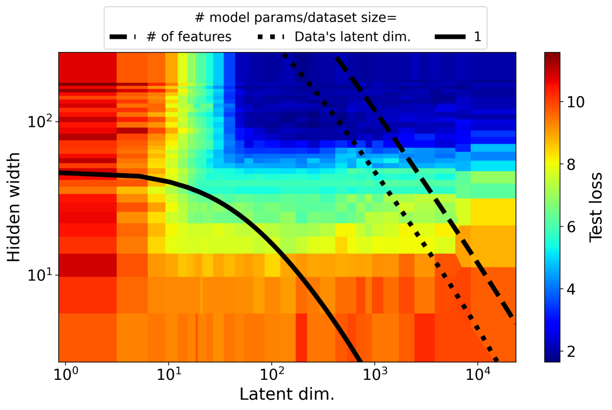
Figure 1: No double descent-like interpolation peak is observed across different latent and hidden widths. When going from a small latent dimension to a high one the loss has a bias-variance-like U-shape. However, when increasing the hidden dimension the loss only decreases. The black lines signify locations where the interpolation peak would be if different output sizes are assumed.

Double descent is a hallmark phenomenon of deep learning, showing the rift between classical learning theory and the generalization capabilities of deep learning systems (Belkin et al., 2019). It manifests as a model’s test loss deviating from the classical U-shape in the bias-variance tradeoff as the model becomes overparameterized (Neal et al., 2018; Belkin et al., 2019; Nakkiran et al., 2019). This form of the phenomenon is known as model-wise double descent, where once the model’s number of parameters is increased the test loss reaches a local maxima known as the interpolation peak. This peak occurs when the number of parameters is approximately equal to the product of the dataset’s size and the dimension of the model’s output, where the model can just interpolate the data (Belkin et al., 2019). After passing the peak the model improves, resulting in the training loss decreasing further and the test loss monotonically decreasing as model capacity increases.

However, previous works study almost only supervised settings. This raises the question, what happens in the self-supervised case? The few works that asked this found that double descent is not as universal as it seemed. For example, Gedon et al. (2023) showed analytically and empirically that double descent does not occur in PCA. Luzi et al. (2021) found that Generative Adversarial Networks (GANs) do not exhibit it either, except in an artificial pseudo-supervised setting. Dar et al. (2020) contrasted the unsupervised and supervised settings by showing that when going from the former to the latter in subspace fitting tasks, double descent gradually appears. Dubova (2022) observed double descent in an autoencoder (AE) but the implications of their results are not obvious as it is unclear whether their task is supervised and the location of their interpolation peak seems to be independent of the model’s capacity.

Following these findings, we hypothesize that double descent does not occur in self-supervised settings. We provide evidence for this claim through an empirical analysis of an autoencoder (AE) (Kramer, 1991; Hinton et al., 2011), showing that it does not exhibit double descent. We choose an AE because of the tension with Dubova (2022)’s results. We hope that our findings will help elucidate the theory of overparameterized models.

2 Experiments

We search for double descent when training an AE on artificial data, akin to the analysis done in Gedon et al. (2023). A detailed overview of the experiment can be found in Appendix A. The dataset $\{\bm{x}_{i}\}_{i=1}^{N}$ is generated through the relation,

$$\bm{x}_{i}=D\bm{z}_{i}+\bm{\epsilon}_{i}$$

where $\bm{z}_{i}\sim\mathcal{N}(0,I_{d})$ are the latent variables, $\bm{\epsilon}_{i}\sim\mathcal{N}(0,I_{n})$ are noise vectors, $n$ is the number of features, $d$ is the latent dimension of the data, and $D_{ij}\sim\mathcal{N}(0,r)$ is a random matrix used to project the latent features into a higher-dimensional space, where $r$ is a constant used to control the signal-to-noise ratio (SNR).

To learn the latent distribution of the data, we used an AE with fully-connected single-layer decoders and encoders, each with the same number of hidden units. The latent layer’s width was varied independently of the hidden layers’ widths because of uncertainty regarding where double descent would occur. Previous results (Dubova, 2022) imply that if double descent occurs in AEs then it might be independent of the hidden width. Although the interpolation peak is where the number of model parameters is equal to the dataset’s size multiplied by the dimension of the output, it is unclear what is the output’s size. For example, one could argue it is the AE’s latent dimension or its number of features. This ambiguity is dealt with by using a wide range of hidden and latent dimensions in the AE to cover both cases. The results are shown in Figure 1. The test loss never exhibits double descent, with its specific behavior depending on how the model was overparameterized.

The training loss corresponding to the results shown in Figure 1 is given in Figure 2. The autoencoder transitions to the interpolation regime in a large part of the parameter space, which is necessary for double descent to occur. This transition happens when the latent dimension is about 20, which is the latent dimension of the data, or when the hidden width is about 28. This could imply that interpolation is possible only when the autoencoder does not have an information bottleneck induced by its layers’ widths.

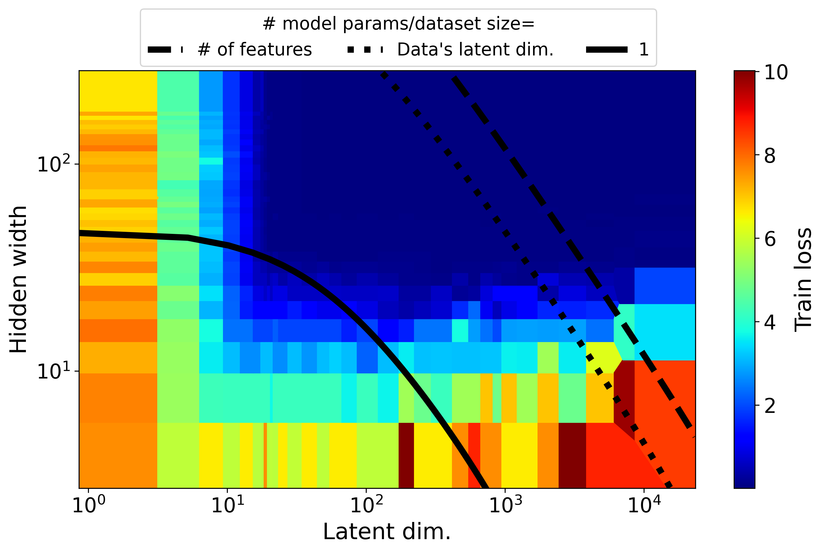
Figure 2: The training loss for the AE experiment. A large part of parameter space is within the interpolation regime.

As double descent is also known to occur in linear regression (Nakkiran, 2019; Derezinski et al., 2019; Bach, 2023), it is natural to test this hypothesis on a similar task. This prompts the use of a linear autoencoder—an autoencoder with no non-linear activation functions. Given the ambiguity in the interpolation peak’s location, this autoencoder’s architecture was kept constant while the dataset size was varied, from being lower than the input dimension to far larger than the number of parameters. The experiments’ hyperparameters are given in Appendix B. The resulting test loss, relative to different parameterization ratios, is shown in Figure 3. No discernible interpolation peak is seen.

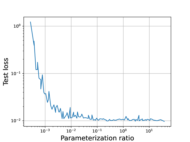
Figure 3: The test loss for different parameterization ratios in the linear AE experiment. Again, no double descent curve is seen.

3 Discussion

We have found evidence that double descent does not occur in self-supervised settings. This hypothesis is based on experiments with a normal and linear autoencoder that add to the literature supporting this finding. The discrepancy between supervised and self-supervised settings may be because of their different formulations—while the former assumes noisy data, in the latter case, the model tries to learn a distribution. A fundamental analysis and more extensive experiments are necessary to test this claim. As a theory is best understood through its shortcomings, we believe that building on these conjectures will help advance our understanding of overparameterized systems.

Appendix A AE Experiment

A.1 Hyperparameters

The parameters used for the data generation and training procedures are given in Table 2. The optimizer used for training was Adam (Kingma and Ba, 2014) and the reconstruction loss was MSE.

Parameter Name	Value
Learning rate	0.001
Epochs	200
Batch size	10
Data’s latent dimension, $d$	20
Number of features, $n$	50
Train dataset size, $N$	5000
Test dataset size	10000
SNR	10

Table 1: Parameters used for the AE experiments.

Parameter Name	Value
Learning rate	$0.001$
Epochs	$1000$
Batch size	$20$
Data’s latent dimension, $d$	$10$
Number of features, $n$	$25$
AE hidden dimension	$100$
AE latent dimension	$20$
Train dataset size, $N$	$8\cdot 10^{0}-1.1\cdot 10^{6}$
Test dataset size	$1000$

Table 2: Parameters used for the linear AE experiments.

A.2 SNR

To control the SNR, $r$ is chosen such that $\frac{\mathbb{E}[||D\bm{z}||_{2}]}{\mathbb{E}[||\bm{\epsilon}||_{2}]}$ has the desired value. As all the random variables are Gaussian, this amounts to setting $r=\frac{\text{SNR}^{2}}{d}$.

A.3 Plot details

The parameter space shown in Figure 1 was not sampled in a linear or logarithmic grid because some regions are expected to have a higher chance of exhibiting double descent than others. To show all the results at once, the parameter space was colored based on the loss of the closest measured point. Logarithmic instead of normal distance is used, so 100 is closer to 1000 than it is to 1.

Appendix B Linear AE Hyperparameters

The experiment’s hyperparameters are given in Table 2. In this setting, the model had $29,445$ trainable parameters.

References

- Bach (2023) Francis R. Bach. High-dimensional analysis of double descent for linear regression with random projections. ArXiv, abs/2303.01372, 2023.
- Belkin et al. (2019) Mikhail Belkin, Daniel Hsu, Siyuan Ma, and Soumik Mandal. Reconciling modern machine-learning practice and the classical bias–variance trade-off. Proceedings of the National Academy of Sciences, 116(32):15849–15854, jul 2019. 10.1073/pnas.1903070116. URL \urlhttps://doi.org/10.1073
- Dar et al. (2020) Yehuda Dar, Paul Mayer, Lorenzo Luzi, and Richard G. Baraniuk. Subspace fitting meets regression: The effects of supervision and orthonormality constraints on double descent of generalization errors, 2020. URL \urlhttps://arxiv.org/abs/2002.10614.
- Derezinski et al. (2019) Michal Derezinski, Feynman T. Liang, and Michael W. Mahoney. Exact expressions for double descent and implicit regularization via surrogate random design. ArXiv, abs/1912.04533, 2019.
- Dubova (2022) Marina Dubova. Generalizing with overly complex representations. In NeurIPS 2022 Workshop on Information-Theoretic Principles in Cognitive Systems, 2022. URL \urlhttps://openreview.net/forum?id=qeu7F3VW8qS.
- Gedon et al. (2023) Daniel Gedon, Antonio H. Ribeiro, and Thomas B. Schön. No double descent in PCA: Training and pre-training in high dimensions, 2023. URL \urlhttps://openreview.net/forum?id=ieWqvOiKgz2.
- Hinton et al. (2011) Geoffrey E Hinton, Alex Krizhevsky, and Sida D Wang. Transforming auto-encoders. In Artificial Neural Networks and Machine Learning–ICANN 2011: 21st International Conference on Artificial Neural Networks, Espoo, Finland, June 14-17, 2011, Proceedings, Part I 21, pages 44–51. Springer, 2011.
- Kingma and Ba (2014) Diederik P. Kingma and Jimmy Ba. Adam: A method for stochastic optimization, 2014. URL \urlhttps://arxiv.org/abs/1412.6980.
- Kramer (1991) Mark A. Kramer. Nonlinear principal component analysis using autoassociative neural networks. Aiche Journal, 37:233–243, 1991.
- Luzi et al. (2021) Lorenzo Luzi, Yehuda Dar, and Richard G. Baraniuk. Double descent and other interpolation phenomena in GANs. CoRR, abs/2106.04003, 2021. URL \urlhttps://arxiv.org/abs/2106.04003.
- Nakkiran (2019) Preetum Nakkiran. More data can hurt for linear regression: Sample-wise double descent, 2019. URL \urlhttps://arxiv.org/abs/1912.07242.
- Nakkiran et al. (2019) Preetum Nakkiran, Gal Kaplun, Yamini Bansal, Tristan Yang, Boaz Barak, and Ilya Sutskever. Deep double descent: Where bigger models and more data hurt, 2019. URL \urlhttps://arxiv.org/abs/1912.02292.
- Neal et al. (2018) Brady Neal, Sarthak Mittal, Aristide Baratin, Vinayak Tantia, Matthew Scicluna, Simon Lacoste-Julien, and Ioannis Mitliagkas. A modern take on the bias-variance tradeoff in neural networks, 2018.