Semi-Elastic LiDAR-Inertial Odometry

Abstract

Existing LiDAR-inertial state estimation methods treats the state at the beginning of current sweep as equal to the state at the end of previous sweep. However, if the previous state is inaccurate, the current state cannot satisfy the constraints from LiDAR and IMU consistently, and in turn yields local inconsistency in the estimated states (e.g., zigzag trajectory or high-frequency oscillating velocity). To address this issue, this paper proposes a semi-elastic LiDAR-inertial state estimation method. Our method provides the state sufficient flexibility to be optimized to the correct value, thus preferably ensuring improved accuracy, consistency, and robustness of state estimation. We integrate the proposed method into an optimization-based LiDAR-inertial odometry (LIO) framework. Experimental results on four public datasets demonstrate that our method outperforms existing state-of-the-art LiDAR-inertial odometry systems in terms of accuracy. In addition, our semi-elastic LiDAR-inertial state estimation method can better enhance the accuracy, consistency, and robustness. We have released the source code of this work to contribute to advancements in LiDAR-inertial state estimation and benefit the broader research community.

I Introduction

3D light detection and ranging (LiDAR) has become the commonly used sensor in robot and autonomous driving fields. In theory, LiDAR-only odometry [28, 29, 16, 2, 19, 20, 8, 7] can achieve pose estimation in real time, and transform the points collected at different times to a unified coordinate system to obtain the global map. However, the Iterative Closest Point (ICP) algorithm used in LiDAR odometry can hardly solve an accurate pose without a reliable initial motion value. Meanwhile, there are not enough geometric features in the scene at all times to provide reliable constraints for pose estimation. By introducing Inertial Measurement Unit (IMU), the above defects can be solved with very low memory and time consumption.

At present, the ICP pose estimation methods utilized in LiDAR odometry are mainly divided into two categories: 1) the widely used ICP algorithm (named traditional ICP algorithm) represented by LOAM [28, 29], which only optimize the pose at the end of a sweep; 2) the elastic ICP algorithm represented by CT-ICP [7]. These two ICP algorithm suffers their own problem when fusing IMU.

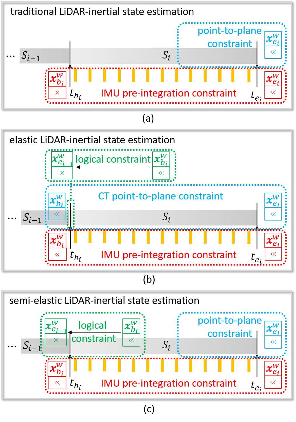
Figure 1: Illustration of (a) traditional LIO optimization, (b) elastic LIO optimization and (c) semi-elastic LIO optimization. Different colors correspond to different constraints on states. $\ll$ means the state can be updated during the optimization, and $\times$ means the state is fixed and cannot be updated.

As illustrated in Fig. 1 (a), the traditional LiDAR-inertial state estimation makes the state at the beginning of current sweep (i.e., $\boldsymbol{x}_{b_{i}}^{w}$) being identical to the state at the end of last sweep (i.e., $\boldsymbol{x}_{e_{i-1}}^{w}$). Thus the state at the end of current sweep (i.e., $\boldsymbol{x}_{e_{i}}^{w}$) is subject to IMU constraints based on $\boldsymbol{x}_{b_{i}}^{w}$($\boldsymbol{x}_{e_{i-1}}^{w}$), which is fixed. If $\boldsymbol{x}_{b_{i}}^{w}$ is inaccurate, the kinematical constraint cannot function correctly. Then the state is not able to satisfy the point-to-plane constraint and the IMU pre-integration [13] constraint at the same time, resulting in local inconsistency of the solved state (e.g., zigzag trajectory or high-frequency oscillating velocity).

Similar as LIWO [27] which extend elastic ICP to elastic LiDAR-inertial-wheel state estimation, the elastic ICP algorithm can be extended to elastic LiDAR-inertial state estimation accordingly. As illustrated in Fig. 1 (b), the elastic LiDAR-inertial state estimation utilize continuous-time (CT) point-to-plane constraint [7] and IMU pre-integration constraint to optimize both $\boldsymbol{x}_{b_{i}}^{w}$ and $\boldsymbol{x}_{e_{i}}^{w}$. Meanwhile, a logical constraint is utilized to make $\boldsymbol{x}_{b_{i}}^{w}$ approach $\boldsymbol{x}_{e_{i-1}}^{w}$ infinitely, while $\boldsymbol{x}_{e_{i-1}}^{w}$ is fixed. The elastic LiDAR-inertial state estimation algorithm is designed to give more elastic space to the state to be optimized. $\boldsymbol{x}_{b_{i}}^{w}$ is not fixed, so it can be updated with IMU pre-integration even if the initial value is inaccurate. Then, $\boldsymbol{x}_{b_{i}}^{w}$ and $\boldsymbol{x}_{e_{i}}^{w}$ are optimized to satisfy the point-to-plane constraint and the IMU pre-integration constraint consistently. However, the logical constraint is not strictly valid and stable at all times. If the irregular geometry (e.g., tree) in the scene causes the CT point-to-plane error large, the weight of the logical constraint will be less relatively. Once the logical constraint is not satisfied, both $\boldsymbol{x}_{b_{i}}^{w}$ and $\boldsymbol{x}_{e_{i}}^{w}$ are not accurate and consistent. If the weight of logical constraint is set too large, the elastic space for states will be insufficient when the geometry in the scene is rich, and the elastic LiDAR-inertial state estimation will degenerate into traditional LiDAR-inertial state estimation.

In this paper, we propose a semi-elastic LiDAR-inertial state estimation method, which is illustrated in Fig. 1 (c). We utilize the point-to-plane constraint to ensure the pose at $t_{e_{i}}$ (i.e., $\boldsymbol{x}_{e_{i}}^{w}$) is accurate, and utilize the logical constraint to make $\boldsymbol{x}_{b_{i}}^{w}$ approach $\boldsymbol{x}_{e_{i-1}}^{w}$ infinitely. The IMU pre-integration constraints both $\boldsymbol{x}_{b_{i}}^{w}$ and $\boldsymbol{x}_{e_{i}}^{w}$ to make them satisfy kinematic constraints within elastic range. Unlike point-to-plane residuals whose error varies greatly with the scene, the error of IMU pre-integration constraint often depends on the noise parameters of the sensor itself. Thus the weight relationship between logical constraint and IMU pre-integration constraint is relatively valid and stable. Meanwhile, the scene-depending point-to-plane constraint cannot affect $\boldsymbol{x}_{b_{i}}^{w}$ directly. Consequently, the logical constraint is always valid and stable. We embed the proposed semi-elastic LiDAR-inertial state estimation into an optimization based LiDAR-inertial odometry (LIO) framework. The experimental results on the public dataset $nclt$ [5], $utbm$ [25], $ulhk$ [22], $kaist$ [10] demonstrate that: 1) our system outperforms existing state-of-the-art LIO systems (i.e., [11, 17, 23, 6]) in term of smaller absolute trajectory error (ATE); 2) the semi-elastic LiDAR-inertial state estimation can better ensure the accuracy, consistency and robustness. The demo video of our supplementary material demonstrates that our system is also compatible with 16-line Robosense LiDAR.

To summarize, the main contributions of this work are three folds: 1) We propose a semi-elastic LiDAR-inertial state estimation method, which can better ensure the accuracy, consistency and robustness of the estimated state; 2) We embed the proposed state estimation into an optimization based LIO system, and achieve the state-of-the-art accuracy; 3) We have release the source code of this work for the development of the community.

The rest of this paper is structured as follows. In Sec. II, we briefly discuss the relevant literature. Sec. III provides preliminaries. Then Sec. IV and Sec. V illustrates the overview and details of our system, followed by experimental evaluation in Sec. VI. Sec. VII concludes the paper.

II Related Work

LiDAR-Only Odometry. LOAM [28] is the earliest LiDAR odometry which is divided into four modules: edge and surface feature extraction, sweep-to-sweep pose estimation, sweep-to-map pose optimization and point cloud registration. LeGO-LOAM [16] proposed to cluster the raw input points into point clusters, and then removed clusters with weak geometric structure information to reduce computation. However, accurately removing clusters with weak geometry is a nontrivial task, and incorrect removal of useful clusters would degrade the accuracy and robustness of pose estimation. In addition, LeGO-LOAM proposed to utilize edge-to-line residuals to constrain 3 horizontal DOF, and utilize point-to-plane residuals to constrain 3 vertical DOF. However, this approach reduces the accuracy and robustness of pose estimation in practice. SuMa [2] proposed to represent the map via a surfel-based representation that aggregates information from points. However, GPU acceleration is necessary for SuMa to achieve real-time performance, and the pose estimation accuracy of SuMa is not better than systems based on the framework of LOAM. Fast-LOAM [19] eliminated the sweep-to-sweep pose estimation module and keep only the sweep-to-map pose estimation module to make the system lightweight. Meanwhile, Fast-LOAM utilized analytic derivative instead of automatic derivation to speed up the Ceres Solver [1]. In [20], authors propose intensity scan context (ISC) to improve the performance of loop detection based on Fast-LOAM. CT-ICP is the first open-sourced elastic LiDAR odometry framework, where the state at the beginning of current sweep and the state at the end of current sweep are variables to be optimized, and a logical constraint is added to make the beginning state approaches to the end state of last sweep. This sweep expression enables to perform pose estimation and the distortion calibration simultaneously. However, adaptively setting the weight of logical constraint is a nontrivial task, and the estimated pose is usually inconsistent if the logical constraint is not strictly satisfied.

LiDAR-Inertial Odometry. LIO-SAM [17] proposed an open-sourced graph optimization based LIO framework, where the state solved by LiDAR ICP is the initial value of the node, and the IMU pre-integration constraint is as the edge. LINs [14] proposed an open-sourced iterated extended Kalman filter (iEKF) based LIO framework. The state is estimated by balancing the weight of the LiDAR ICP constraint and the IMU pre-integration constraint according to the iteratively updated Kalman gain. Fast-LIO [24] utilized the mathematical technique [18] to optimize the process of solving Kalman gain, which converts the inverse calculation of the $N$-dimensional matrix to $18$-dimensional matrix, where $N$ is the number of point-to-plane residuals and $18$ is the dimensional of state vector. This transformation greatly speeds up the solving speed, and makes more point-to-plane residual terms can be added to LIO optimization framework, thus improving the accuracy. Fast-LIO2 [23] proposed to build point-to-plane residuals directly on down-sampled input points. At the same time, the ikdtree [4] is proposed to manage the map. Compared to the traditional kdtree, the ikdtree takes less time to traverse, add, and delete elements. DLIO [6] proposed to retain a 3-order minimum in state prediction and point distortion calibration to obtain more accurate pose estimation results.

In addition to the above single sweep-to-map approaches, there are several LIO systems that use multi-sweep joint optimization framework. LIO_mapping [26] is an open-sourced LIO system based on bundle adjustment (BA) framework. It utilized a multi-sweep joint optimization framework similar to VINs-Mono [15] to ensure the accuracy of state estimation, however, the resulting large computational load causes LIO_mapping cannot run in real time (but closer to real time). LiLi-OM [11] selects some representative key-sweeps from original sweeps, and performs multi-sweep joint optimization to optimize the state of key-sweeps. However, the real-time performance cannot be guaranteed steadily. LIO_Livox [12] is an official open-sourced LIO framework proposed by Livox company. For the point cloud of input sweep, the dynamic points are removed, and the edge, surface and irregular features are extracted. Then the state is estimated by multi-sweep joint optimization. However, the official LIO_Livox cannot ensure the real-time performance if utilizing more than 3 sweeps to perform multi-joint LIO optimization. Ssl_slam3 [21] utilized the point-to-plane constraints from of a single sweep and IMU pre-integration constraints from multiple sweeps to improve real-time performance. All of above systems utilized multi-sweep joint optimization to perform LIO state estimation. Because in addition to eliminating accumulated errors, multi-sweep joint optimization gives sufficient elasticity to state, making them more likely to update to the correct value. However, introducing more variables and residuals will also increase the amount of computation, so the side effect is also very significant. By contrast, our semi-elastic LIO optimization framework avoids additional computation while providing enough elasticity for state variables.

III Preliminary

III-A Coordinate Systems

We denote $(\cdot)^{w}$, $(\cdot)^{l}$ and $(\cdot)^{o}$ as a 3D point in the world coordinates, the LiDAR coordinates and the IMU coordinates respectively. The world coordinate is coinciding with $(\cdot)^{o}$ at the starting position.

We denote the LiDAR coordinate for taking the $i_{th}$ sweep at time $t_{i}$ as $l_{i}$ and the corresponding IMU coordinate at $t_{i}$ as $o_{i}$, then the transformation matrix (i.e., external parameters) from $l_{i}$ to $o_{i}$ is denoted as $\mathbf{T}_{l_{i}}^{o_{i}}\in SE(3)$:

$$\mathbf{T}_{l_{i}}^{o_{i}}=\left[\begin{array}[]{cc}\mathbf{R}_{l_{i}}^{o_{i}}&\mathbf{t}_{l_{i}}^{o_{i}}\\ \mathbf{0}&1\end{array}\right]$$ (1)

where $\mathbf{T}_{l_{i}}^{o_{i}}$ consists of a rotation matrix $\mathbf{R}_{l_{i}}^{o_{i}}\in SO(3)$ and a translation vector $\mathbf{t}_{l_{i}}^{o_{i}}\in\mathbb{R}^{3}$. The external parameters are usually calibrated once offline and remain constants during online state estimation; therefore, we can represent $\mathbf{T}_{l_{i}}^{o_{i}}$ using $\mathbf{T}_{l}^{o}$ for simplicity. In the following statement, we omit the index that represents the coordinate system for simplified notation. For instance, the pose from the IMU coordinate to the world coordinate is strictly defined as $\mathbf{T}_{o_{i}}^{w}$. Now we define it as $\mathbf{T}_{i}^{w}$ for simplify.

In addition to pose, we also estimate the velocity $\mathbf{v}$, the accelerometer bias ${\mathbf{b}}_{\mathbf{a}}$ and the gyroscope bias ${\mathbf{b}}_{\boldsymbol{\omega}}$, which are represented uniformly by a state vector:

$$\boldsymbol{x}=\left[\mathbf{t}^{T},\mathbf{q}^{T},\mathbf{v}^{T},\mathbf{b}_{\mathbf{a}}{}^{T},\mathbf{b}_{\boldsymbol{\omega}}{}^{T}\right]^{T}$$ (2)

where $\mathbf{q}$ is the quaternion form of the rotation matrix $\mathbf{R}$.

III-B IMU Measurement Model

A IMU consists of an accelerometer and a gyroscope. The raw accelerometer and gyroscope measurements from IMU, $\hat{\mathbf{a}}_{t}$ and $\hat{\boldsymbol{\omega}}_{t}$, are given by:

$$\begin{gathered}\hat{\mathbf{a}}_{t}=\mathbf{a}_{t}+\mathbf{b}_{\mathbf{a}_{t}}+\mathbf{R}_{w}^{t}\mathbf{g}^{w}+\mathbf{n}_{\mathbf{a}}\\ \hat{\boldsymbol{\omega}}_{t}=\boldsymbol{\omega}_{t}+\mathbf{b}_{\boldsymbol{\omega}_{t}}+\mathbf{n}_{\boldsymbol{\omega}}\end{gathered}$$ (3)

IMU measurements, which are measured in IMU coordinates, combine the force for countering gravity and the platform dynamics, and are affected by acceleration bias $\mathbf{b}_{\mathbf{a}_{t}}$, gyroscope bias $\mathbf{b}_{\boldsymbol{\omega}_{t}}$, and additive noise. As mentioned in VINs-Mono [15], the additive noise in acceleration and gyroscope measurements are modeled as Gaussian white noise, $\mathbf{n}_{\mathbf{a}}\sim N\left(\mathbf{0},\boldsymbol{\sigma}_{\mathbf{a}}^{2}\right)$, $\mathbf{n}_{\boldsymbol{\omega}}\sim N\left(\mathbf{0},\boldsymbol{\sigma}_{\boldsymbol{\omega}}^{2}\right)$. Acceleration bias and gyroscope bias are modeled as random walk, whose derivatives are Gaussian, $\dot{\mathbf{b}}_{\mathbf{a}_{t}}=\mathbf{n}_{\mathbf{b}_{\mathbf{a}}}\sim N\left(\mathbf{0},\boldsymbol{\sigma}_{\mathbf{b}_{\mathbf{a}}}^{2}\right)$, $\dot{\mathbf{b}}_{{\boldsymbol{\omega}}_{t}}=\mathbf{n}_{\mathbf{b}_{\boldsymbol{\omega}}}\sim N\left(\mathbf{0},\boldsymbol{\sigma}_{\mathbf{b}_{\boldsymbol{\omega}}}^{2}\right)$.

III-C Sweep State Expression

The same as CT-ICP [7], we represent the state of a sweep $S$ by: 1) the state at the beginning time $t_{b}$ of $S$ (e.g., $\boldsymbol{x}_{b}$) and 2) the state at the end time $t_{e}$ of $S$ (e.g., $\boldsymbol{x}_{e}$). There are two ways for LiDAR point distortion calibration in our system: utilizing IMU integrated pose to calibrate or utilizing uniform motion model. For vehicle platforms that are mostly in uniform motion state, we recommend the uniform motion distortion calibration model because IMU measurements are sometimes affected by large noise.

IV System Overview

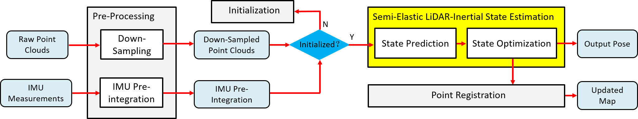
Figure 2: Overview of our LIO system which consists of four main modules: a pre-processing module, an initialization module, a semi-elastic LiDAR-inertial state estimation module and a point registration module. The yellow part is the core contribution we proposed.

Fig. 2 illustrates the framework of our system which consists of four main modules: a pre-processing module, an initialization module, a semi-elastic LiDAR-inertial state estimation module and a point registration module. The pre-processing module takes sensor raw data as input, and outputs down-sampled point clouds and IMU pre-integration. The initialization module is used to estimate some state parameters such as gravitational acceleration, accelerometer bias, gyroscope bias, and initial velocity. The semi-elastic LiDAR-inertial state estimation module executes state prediction and state optimization in turn, which is detailed in Sec. V-C. After state estimation, the point registration adds the new points to the map and delete the points that are far away from current position.

V System Details

V-A Pre-processing

V-A1 Down-Sampling

The down-sampling module can be divided into quantitative down-sampling and spatial down-sampling. The quantitative down-sampling strategy keep only one out of every four points to reduce the computational complexity. Then we follow the strategy utilized by CT-ICP to perform the spatial down-sampling to ensure that the density distribution of points is uniform.

V-A2 IMU Pre-integration

Typically, the IMU sends out data at a much higher frequency than the LiDAR. Pre-integration of all IMU measurements between two consecutive sweeps $S_{i}$ and $S_{i+1}$ can well summarize the dynamics of the hardware platform from time $t_{e_{i}}$ to $t_{e_{i+1}}$, where $e_{i}$ and $e_{i+1}$ are the end time stamp of $S_{i}$ and $S_{i+1}$ respectively. In this work, we employ the discrete-time quaternion-based derivation of IMU pre-integration approach [13], and incorporate IMU bias using the method in [15]. Specifically, the pre-integrations between $S_{i}$ and $S_{i+1}$ in the corresponding IMU coordinates $o_{e_{i}}$ and $o_{e_{i+1}}$, i.e., $\hat{\boldsymbol{\alpha}}_{e_{i+1}}^{e_{i}}$, $\hat{\boldsymbol{\beta}}_{e_{i+1}}^{e_{i}}$, and $\hat{\boldsymbol{\gamma}}_{e_{i+1}}^{e_{i}}$, are calculated, where $\boldsymbol{\alpha}_{e_{i+1}}^{e_{i}}$, $\boldsymbol{\beta}_{e_{i+1}}^{e_{i}}$, $\boldsymbol{\gamma}_{e_{i+1}}^{e_{i}}$ are the pre-integration of translation, velocity, rotation from IMU measurements respectively. In addition, the Jacobian of pre-integration with respect to bias, i.e., $\mathbf{J}_{\mathbf{b}_{\mathbf{a}}}^{\boldsymbol{\alpha}}$, $\mathbf{J}_{\mathbf{b}_{\boldsymbol{\omega}}}^{\boldsymbol{\alpha}}$, $\mathbf{J}_{\mathbf{b}_{\mathbf{a}}}^{\boldsymbol{\beta}}$, $\mathbf{J}_{\mathbf{b}_{\boldsymbol{\omega}}}^{\boldsymbol{\beta}}$, $\mathbf{J}_{\mathbf{b}_{\boldsymbol{\omega}}}^{\boldsymbol{\gamma}}$, are also calculated according to the error state kinematics.

V-B Initialization

The initialization module aims to estimate all necessary values including initial pose, velocity, gravitational acceleration, accelerometer bias and gyroscope bias, for subsequent state estimation. We adopt static initialization in our system. Please refer to [9] for more details about our initialization module.

V-C Semi-Elastic LiDAR-Inertial State Estimation

V-C1 State Prediction

When every new down-sampled sweep $P_{i+1}$ completes, we use IMU measurements to predict the state at the beginning of $P_{i+1}$ (i.e., $\boldsymbol{x}_{b_{i+1}}^{w}$) and the state at the end of $P_{i+1}$ (i.e., $\boldsymbol{x}_{e_{i+1}}^{w}$), which are provided as the prior motion for LIO-optimization. Specifically, the predicted state $\boldsymbol{x}_{b_{i+1}}^{w}$ (i.e., $\mathbf{t}_{b_{i+1}}^{w}$, $\mathbf{R}_{b_{i+1}}^{w}$, $\mathbf{v}_{b_{i+1}}^{w}$, ${\mathbf{b}}_{\mathbf{a}_{b_{i+1}}}$ and ${\mathbf{b}}_{\boldsymbol{\omega}_{b_{i+1}}}$) is assigned as:

$$\boldsymbol{x}_{b_{i+1}}^{w}=\boldsymbol{x}_{e_{i}}^{w}$$ (4)

and $\boldsymbol{x}_{e_{i+1}}^{w}$ (i.e., $\mathbf{t}_{e_{i+1}}^{w}$, $\mathbf{R}_{e_{i+1}}^{w}$, $\mathbf{v}_{e_{i+1}}^{w}$, ${\mathbf{b}}_{\mathbf{a}_{e_{i+1}}}$ and ${\mathbf{b}}_{\boldsymbol{\omega}_{e_{i+1}}}$) is calculated as:

$$\begin{gathered}\mathbf{R}_{n+1}^{w}=\mathbf{R}_{n}^{w}Exp\left(\left(\frac{\hat{\boldsymbol{\omega}}_{n}+\hat{\boldsymbol{\omega}}_{n+1}}{2}-\mathbf{b}_{\boldsymbol{\omega}_{e_{i}}}\right)\delta t\right)\\ \mathbf{v}_{n+1}^{w}=\mathbf{v}_{n}^{w}+\left(\frac{\hat{\mathbf{a}}_{n}+\hat{\mathbf{a}}_{n+1}}{2}-\mathbf{b}_{\mathbf{a}_{e_{i}}}-\mathbf{R}_{w}^{n}\mathbf{g}^{w}\right)\delta t\\ \mathbf{t}_{n+1}^{w}=\mathbf{t}_{n}^{w}+\mathbf{v}_{n}^{w}\delta t+\frac{1}{2}\left(\frac{\hat{\mathbf{a}}_{n}+\hat{\mathbf{a}}_{n+1}}{2}-\mathbf{b}_{\mathbf{a}_{e_{i}}}-\mathbf{R}_{n}^{w}\mathbf{g}^{w}\right)\delta t^{2}\end{gathered}$$ (5)

where $\mathbf{g}^{w}$ is the gravitational acceleration in world coordinates, $n$ and $n+1$ are two time instants of obtaining an IMU measurement during $\left[t_{e_{i}},t_{e_{i+1}}\right]$, $\delta t$ is the time interval between $n$ and $n+1$. We iteratively increase $n$ from $0$ to $\left(t_{e_{i+1}}-t_{e_{i}}\right)/\delta t$ to obtain $\boldsymbol{x}_{e_{i+1}}^{w}$. When $n=0$, $\boldsymbol{x}_{n}^{w}=\boldsymbol{x}_{e_{i}}^{w}$. For $\mathbf{b}_{\mathbf{a}_{e_{i+1}}}$ and $\mathbf{b}_{\boldsymbol{\omega}_{e_{i+1}}}$, we set the predicted values of them by: $\mathbf{b}_{\mathbf{a}_{e_{i+1}}}=\mathbf{b}_{\mathbf{a}_{e_{i}}}$ and $\mathbf{b}_{\boldsymbol{\omega}_{e_{i+1}}}=\mathbf{b}_{\boldsymbol{\omega}_{e_{i}}}$.

V-C2 State Optimization

We jointly utilize measurements of the LiDAR and IMU to optimize the beginning state (i.e., $\boldsymbol{x}_{b_{i+1}}^{w}$) and the end state (i.e., $\boldsymbol{x}_{e_{i+1}}^{w}$) of the current sweep $P_{i+1}$, where the variable vector is expressed as:

$$\boldsymbol{\chi}=\left\{\boldsymbol{x}_{b_{i+1}}^{w},\boldsymbol{x}_{e_{i+1}}^{w}\right\}$$ (6)

Residual from the LiDAR constraint. For a distortion-calibrated point $\mathbf{p}$, we first project $\mathbf{p}$ to the world coordinate to obtain $\mathbf{p}^{w}$, and then find 20 nearest points around $\mathbf{p}^{w}$ from the volume. To search for the nearest neighbor of $\mathbf{p}^{w}$. We only search in the voxel $V$ to which $\mathbf{p}^{w}$ belongs, and the 8 voxels adjacent to $V$. The 20 nearest points are used to fit a plane with a normal $\mathbf{n}$ and a distance $d$. Accordingly, we can build the point-to-plane residual $r^{\mathbf{p}}$ for $\mathbf{p}$ as:

$$\begin{gathered}r^{\mathbf{p}}=\omega_{\mathbf{p}}\left(\mathbf{n}^{T}\mathbf{p}^{w}+d\right)\\ \mathbf{p}^{w}=\mathbf{q}_{e_{i+1}}^{w}\mathbf{p}+\mathbf{t}_{e_{i+1}}^{w}\end{gathered}$$ (7)

where $\omega_{\mathbf{p}}$ is a weight parameter utilized in [7], $\mathbf{q}_{e_{i+1}}^{w}$ is the rotation with respect to $(\cdot)^{w}$ at $t_{e_{i+1}}$, $\mathbf{t}_{e_{i+1}}^{w}$ is the translation with respect to $(\cdot)^{w}$ at $t_{e_{i+1}}$. Both $\mathbf{q}_{e_{i+1}}^{w}$, $\mathbf{t}_{e_{i+1}}^{w}$ are variables to be refined, and the initial value of them are obtained from Sec. V-C1.

Residual from the IMU constraint. Considering the IMU measurements during $\left[t_{e_{i}},t_{e_{i+1}}\right]$, according to pre-integration introduced in Sec. V-A2, the residual for pre-integrated IMU measurements can be computed as:

$$\begin{gathered}{{\mathbf{r}_{o}}_{{e_{i+1}}}^{b_{i+1}}}=\\ {\left[\begin{array}[]{c}\mathbf{R}_{w}^{b_{i+1}}\left(\mathbf{t}_{e_{i+1}}^{w}-\mathbf{t}_{b_{i+1}}^{w}+\frac{1}{2}\mathbf{g}^{w}\Delta t^{2}-\mathbf{v}_{b_{i+1}}^{w}\Delta t\right)-\hat{\boldsymbol{\alpha}}_{e_{i+1}}^{e_{i}}\\ \mathbf{R}_{w}^{b_{i+1}}\left(\mathbf{v}_{e_{i+1}}^{w}+\mathbf{g}^{w}\Delta t-\mathbf{v}_{b_{i+1}}^{w}\right)-\hat{\boldsymbol{\beta}}_{e_{i+1}}^{e_{i}}\\ 2\left[\mathbf{q}_{b_{i+1}}^{{w}^{-1}}\otimes\mathbf{q}_{e_{i+1}}^{w}\otimes\left(\hat{\boldsymbol{\gamma}}_{e_{i+1}}^{e_{i}}\right)^{-1}\right]_{xyz}\\ \mathbf{b}_{\mathbf{a}_{i+1}}-\mathbf{b}_{\mathbf{a}_{i}}\\ \mathbf{b}_{\boldsymbol{\omega}_{i+1}}-\mathbf{b}_{\boldsymbol{\omega}_{i}}\end{array}\right]}\end{gathered}$$ (8)

where $[\cdot]_{xyz}$ extracts the vector part of a quaternion q for error state representation. At the end of each iteration, we update $\left[\hat{\boldsymbol{\alpha}}_{e_{i+1}}^{e_{i}},\hat{\boldsymbol{\beta}}_{e_{i+1}}^{e_{i}},\hat{\boldsymbol{\gamma}}_{e_{i+1}}^{e_{i}}\right]^{T}$ with the first order Jacobian approximation [15].

Residual from the consistency constraint. $\boldsymbol{x}_{b_{i+1}}^{w}$ and $\boldsymbol{x}_{e_{i}}^{w}$ are two states at the same time stamp $t_{b_{i+1}}$($t_{e_{i}}$). Logically, $\boldsymbol{x}_{e_{i}}^{w}$ and $\boldsymbol{x}_{b_{i+1}}^{w}$ should be the same. Therefore, we build the consistency residual as follow:

$$\mathbf{r}_{c}=\left[\begin{array}[]{c}\mathbf{r}_{c}^{\mathbf{t}}\\ \mathbf{r}_{c}^{\mathbf{q}}\\ \mathbf{r}_{c}^{\mathbf{v}}\\ \mathbf{r}_{c}^{\mathbf{b}_{\mathbf{a}}}\\ \mathbf{r}_{c}^{\mathbf{b_{\boldsymbol{\omega}}}}\end{array}\right]=\left[\begin{array}[]{c}\mathbf{t}_{b_{i+1}}^{w}-\mathbf{t}_{e_{i}}^{w}\\ 2\left[{\mathbf{q}_{e_{i}}^{w}}^{-1}\otimes\mathbf{q}_{b_{i+1}}^{w}\right]_{xyz}\\ \mathbf{v}_{b_{i+1}}^{w}-\mathbf{v}_{e_{i}}^{w}\\ \mathbf{b}_{\mathbf{a}_{b_{i+1}}}-\mathbf{b}_{\mathbf{a}_{e_{i}}}\\ \mathbf{b}_{\boldsymbol{\omega}_{b_{i+1}}}-\mathbf{b}_{\boldsymbol{\omega}_{e_{i}}}\end{array}\right]$$ (9)

where $\mathbf{t}_{b_{i+1}}^{w}$, $\mathbf{q}_{b_{i+1}}^{w}$, $\mathbf{v}_{b_{i+1}}^{w}$, $\mathbf{b}_{\mathbf{a}_{b_{i+1}}}$, $\mathbf{b}_{\boldsymbol{\omega}_{b_{i+1}}}$ are varibales to be optimized.

By minimizing the sum of point-to-plane residuals, the IMU pre-integration residuals, and the consistency residuals, we maximize a posteriori estimation as:

$$\begin{gathered}\boldsymbol{\chi}=\min_{\boldsymbol{\chi}}\\ \left\{\rho\left(\sum_{\mathbf{p}\in P_{i+1}}\left\|r^{\mathbf{p}}\right\|_{\mathbf{P}_{L}}^{2}+\left\|{\mathbf{r}_{o}}_{e_{i+1}}^{b_{i+1}}\right\|_{\mathbf{P}_{e_{i+1}}^{e_{i}}}^{2}+\left\|\mathbf{r}_{c}\right\|^{2}\right)\right\}\end{gathered}$$ (10)

where $\rho$ is the Huber kernel to eliminate the influence of outlier residuals. $\mathbf{P}_{e_{i+1}}^{e_{i}}$ is the covariance matrix of pre-integrated IMU measurements. The inverse of $\mathbf{P}_{e_{i+1}}^{e_{i}}$ is utilized as the weight of IMU pre-integration residuals. $\mathbf{P}_{L}$ is a constant (e.g., 0.001 in our system) to indicate the reliability of the point-to-plane residuals. The inverse of $\mathbf{P}_{L}$ is utilized as the weight of point-to-plane residuals. After finishing the state optimization, we selectively add the points of current sweep to the map.

V-D Point Registration

Following CT-ICP [7], the cloud map is stored in a volume, and the size of each voxel is 1.0$\times$1.0$\times$1.0 (unit: m). Each voxel contains a maximum of 20 points. When the state of current down-sampled sweep $P_{i+1}$ has been estimated, we transform $P_{i+1}$ to the world coordinate system $(\cdot)^{w}$, and add the transformed points into the volume map. If a voxel already has 20 points, the new points cannot be added to it. Meanwhile, we delete the points that are far away from current position.

VI Experiments

TABLE I: Datasets for Evaluation

	Velodyne LiDAR		IMU
	Type	Rate	Type	Rate
nclt	32	7.5	9-axis	100 Hz
utbm	32	10	6-axis	100 Hz
ulhk	32	10	9-axis	100 Hz
kaist	16	10	9-axis	200 Hz

TABLE II: Datasets of All Sequences for Evaluation

	Name	Duration (min:sec)	Distance (km)
$nclt\_1$	2012-01-08	92:16	6.4
$nclt\_2$	2012-01-22	86:11	6.1
$nclt\_3$	2012-02-04	77:39	5.5
$nclt\_4$	2012-02-05	93:40	6.5
$nclt\_5$	2012-02-12	85:17	5.8
$nclt\_6$	2012-03-17	81:51	5.8
$nclt\_7$	2012-04-29	43:17	3.1
$nclt\_8$	2012-05-11	83:36	6.0
$nclt\_9$	2012-05-26	97:23	6.3
$nclt\_10$	2012-06-15	55:10	4.1
$nclt\_11$	2012-08-04	79:27	5.5
$nclt\_12$	2012-08-20	88:44	6.0
$nclt\_13$	2012-09-28	76:40	5.6
$nclt\_14$	2012-11-04	79:53	4.8
$nclt\_15$	2012-12-01	75:50	5.0
$nclt\_16$	2013-01-10	17:02	1.1
$utbm\_1$	2018-07-19	15:26	4.98
$utbm\_2$	2019-01-31	16:00	6.40
$utbm\_3$	2019-04-18	11:59	5.11
$utbm\_4$	2018-07-20	16:45	4.99
$utbm\_5$	2018-07-17	15:59	4.99
$utbm\_6$	2018-07-16	15:59	4.99
$utbm\_7$	2018-07-13	16:59	5.03
$ulhk\_1$	2019-01-17	5:18	0.60
$ulhk\_2$	2019-04-26-1	2:30	0.55
$kaist\_1$	urban_07	9:16	2.55
$kaist\_2$	urban_08	5:07	1.56
$kaist\_3$	urban_13	24:14	2.36

We evaluated our system on the public datasets $nclt$ [5], $utbm$ [25], $ulhk$ [22] and $kaist$ [10]. $nclt$ is a large-scale, long-term autonomy unmanned ground vehicle dataset collected in the University of Michigans North Campus. The $nclt$ dataset contains a full data stream from a Velodyne HDL-32E LiDAR and 50 Hz data from Microstrain MS25 IMU. The $nclt$ dataset has a much longer duration and amount of data than other datasets and contains several open scenes, such as a large open parking lot. Different from the other three datasets (e.g., $utbm$, $ulhk$ and $kaist$), the LiDAR of $nclt$ need 130$\sim$140 ms to finish a 360 deg sweep, which means the frequency of sweep is around 7.5 Hz. In addition, 50 Hz IMU measurements cannot meet the requirements of some systems (e.g., LIO-SAM [17]). Therefore, we increase the frequency of the IMU to 100 Hz by interpolation. The $utbm$ dataset is collected with a human-driving robocar in maximum 50 km/h speed, which has two 10 Hz Velodyne HDL-32E LiDAR5 and 100 Hz Xsens MTi-28A53G25 IMU. For point clouds, we only utilize the data from the left LiDAR. $ulhk$ contains 10 Hz LiDAR sweep from Velodyne HDL-32E and 100 Hz IMU data from a 9-axis Xsens MTi-10 IMU. $kaist$ contains two 10 Hz Velodyne VLP-16, 200 Hz Ssens MTi-300 IMU and 100 Hz RLS LM13 wheel encoder. Two 3D LiDARs are tilted by approximately $45^{\circ}$. For point clouds, we utilize the data from both two 3D LiDARs. All the sequences of $utbm$, $ulhk$ and $kaist$ are collected in structured urban areas by a human-driving vehicle. The datasets’ information, including the sensors’ type and data rate, are illustrated in Table I. Due to the above three datasets both utilize the vehicle platform, we utilize uniform motion distortion calibration model in our system. The details about all the 28 sequences used in this section, including name, duration, and distance, are listed in Table II. For all four datasets, we utilize the universal evaluation metrics – absolute translational error (ATE) as the evaluation metrics. A consumer-level computer equipped with an Intel Core i7-12700 and 32 GB RAM is used for all experiments.

VI-A Comparison of the State-of-the-Arts

TABLE III: RMSE of ATE Comparison of State-of-the-art (Unit: m)

	LiLi-OM	LIO-SAM	Fast-LIO2	DLIO	Ours
$nclt\_1$	50.71	1.85*	3.57	3.27	1.76
$nclt\_2$	91.20	9.70*	2.24	2.82	1.82
$nclt\_3$	92.93	2.16*	2.77	5.35*	1.85
$nclt\_4$	215.91	2.70*	3.60	18.10*	1.55
$nclt\_5$	145.52	2.74*	5.23	2.01*	1.82
$nclt\_6$	262.30	$\times$	3.04	6.39	2.17
$nclt\_7$	93.61	1.75	1.40	1.51	1.38
$nclt\_8$	185.24	$\times$	2.46	3.14	2.20
$nclt\_9$	141.83	$\times$	2.60	12.44	2.22
$nclt\_10$	50.42	2.97	2.37	2.98	2.24
$nclt\_11$	137.05	2.26*	2.59	7.84	2.25
$nclt\_12$	224.68	10.68*	4.01	2.46	2.23
$nclt\_13$	$\times$	$\times$	2.65	7.72	2.13
$nclt\_14$	229.66	7.89*	3.83	3.15	2.19
$nclt\_15$	$\times$	$\times$	4.37	3.89	2.16
$nclt\_16$	$\times$	1.78	0.90	0.91	0.92
$utbm\_1$	67.16	-	15.13	14.25	15.27
$utbm\_2$	38.17	-	21.21	13.85	18.58
$utbm\_3$	10.70	-	10.81	55.28	10.16
$utbm\_4$	70.98	-	15.20	18.05	13.44
$utbm\_5$	86.80	-	13.16	12.66	11.71
$utbm\_6$	84.77	-	14.67	13.42	13.40
$utbm\_7$	62.57	-	13.24	14.95	12.15
$ulhk\_1$	$\times$	1.68	1.20	2.44	0.93
$ulhk\_2$	3.11	3.13	3.24	$\times$	3.24
$kaist\_1$	$\times$	16.96	0.88	1.04	0.86
$kaist\_2$	$\times$	$\times$	16.27	1.91	3.44
$kaist\_3$	$\times$	$\times$	$\times$	$\times$	1.04

We compare our system with four state-of-the-art LIO systems, i.e., LiLi-OM [11], LIO-SAM [17], Fast-LIO2 [23] and DLIO [6]. LiLi-OM selects key-sweeps from raw input sweeps, and joint the constraints from LiDAR and IMU in a multi-sweep joint optimization framework. LIO-SAM joints the IMU factor and the LiDAR point-to-plane factor into a graph optimization based framework. Both Fast-LIO2 and DLIO are iEKF framework based LIO systems, where Fast-LIO2 utilizes the ikdtree [4] and DLIO utilizes the nanoflan [3] to manage the map. For a fair comparison, we obtain the results of above systems based on the source code provided by the authors.

Results in Table III demonstrate that our system outperforms LiLi-OM, LIO-SAM and Fast-LIO2 for almost all sequences in terms of smaller ATE. Although our accuracy is not the best on $nclt\_16$ and $ulhk\_2$, we are very close to the best accuracy, where the ATE is only 2 cm more on $nclt\_16$ and 13 cm more on $ulhk\_4$. “-” means the corresponding value is not available. LIO-SAM needs 9-axis IMU data as imput, while the utbm dataset only provides 6-axis IMU data. Therefore, we cannot provide the results of LIO-SAM on $utbm$ dataset. “$\times$” means the system fails to run entirety on the corresponding sequence, and “*” means the system crashes towards the end of this sequence. Although DLIO achieves more accurate results than our system on some sequences (i.e., $utbm\_1$, $utbm\_2$ and $kaist\_2$), it cannot run completely on more sequences or can run but achieve a huge ATE error (i.e., $nclt\_3$, $nclt\_4$, $nclt\_5$, $nclt\_9$, $utbm\_3$, $ulhk\_2$ and $kaist\_3$). LiLi-OM and LIO-SAM fails or crashes on most sequences, and the state-of-the-art Fast-LIO also fails on $kaist\_3$ and achieves a huge ATE error on $kaist\_2$. In contrast, our system can run properly on almost all sequences, which also demonstrates the good robustness of our system.

VI-B Ablation Study of Semi-Elastic State Estimation

TABLE IV: Ablation Study of Semi-Elastic State Estimation on Accuracy

	traditional	elastic	semi-elastic
$nclt\_16$	0.95	0.92	0.92
$utbm\_6$	13.53	$\times$	13.45
$ulhk\_1$	1.54	1.03	0.93
$kaist\_3$	76.94	$\times$	1.04

We examine the effectiveness of our proposed semi-elastic state estimation on accuracy by comparing the ATE result utilizing the traditional LiDAR-inertial state estimation, the elastic LiDAR-inertial state estimation and the semi-elastic LiDAR-inertial state estimation. We use one sequence from each of the four datasets to complete the evaluation of this ablation experiment. Results in Table IV demonstrate that the proposed semi-elastic LiDAR-inertial state estimation can greatly improve the accuracy and robustness of our system.

In addition, we also examine the effectiveness of our method on consistency by comparing the smoothness of estimated trajectory and the curve of estimated velocity. In theory, the estimated trajectory should be smooth but not zigzag. If there is a zigzag somewhere, the consistency of estimated state there is very poor. As illustrated in Fig. 3, the local trajectory with zigzag shape is easy to appear utilizing traditional LiDAR-inertial state estimation method, which means the strong local inconsistency. The trajectory corresponding to elastic LiDAR-inertial state estimation drifts directly. By contrast, our semi-elastic LiDAR-inertial state estimation can obtain a smooth trajectory.

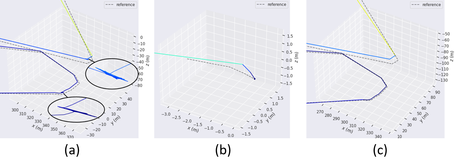
Figure 3: (a) The local zigzag of trajectory estimated by traditional LiDAR-inertial state estimation. (b) The drifting trajectory estimated by elastic LiDAR-inertial state estimation. (c) The smooth trajectory estimated by our semi-elastic LiDAR-inertial state estimation.

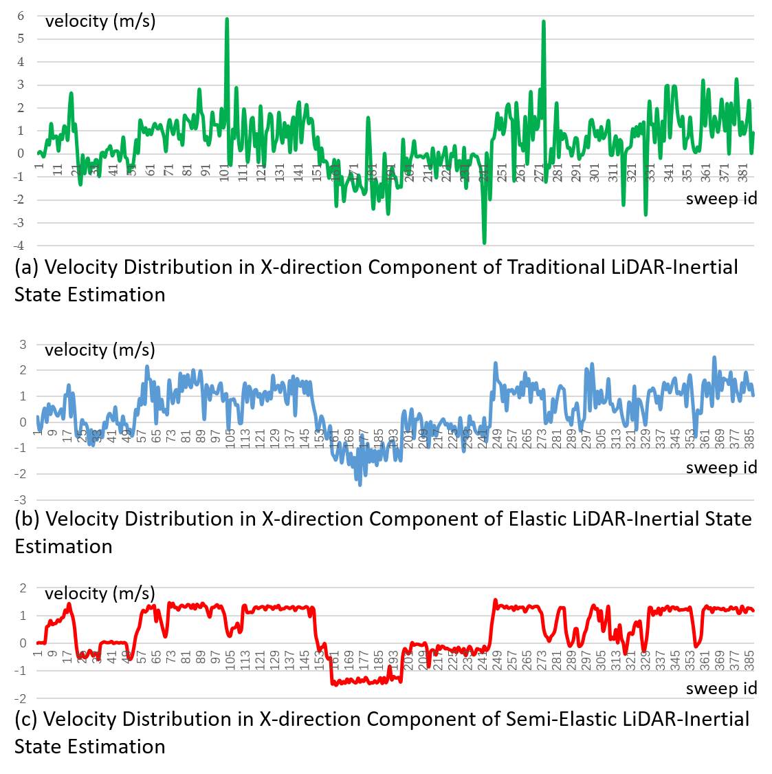
Figure 4: The curve of estimated velocity in X-direction Component by three state estimation methods on $nclt\_16$. We downsampled the sample size by 1/20 when plotting.

In practice, it is difficult for us to obtain the ground truth value of velocity. However, we can still make a stereotypical evaluation of the accuracy of velocity based on the kinematic attempt. In theory, the velocity of a moving vehicle should be continuous and smooth, but not oscillating at a high frequency. Therefore, the smoother the curve of a velocity function with respect to time, the better the curve fits the kinematics attempt. We utilize the sequence $nclt\_16$ as example. As illustrated in Fig. 4, compared to the high frequency oscillation curve of traditional and elastic LiDAR-inertial state estimation, the curve of proposed semi-elastic LiDAR-inertial state estimation is much smoother. That means there is still a gap in consistency even if the ATE of estimated pose by the three methods is similar (recorded in Table IV). In addition, although the groundtruth of velocity vector cannot be obtained, the nclt dataset has the observation from wheel odometer encoder to provide the magnitude of velocity whose maximum value is 1.5m/s on $nclt\_16$, which is also in good agreement with the velocity curve estimated by our method. This shows that our method can not only ensure the consistency, but also greatly improve the accuracy of estimated velocity, demonstrating the effectiveness of semi-elastic LiDAR-inertial state estimation method.

VI-C Time Consumption

TABLE V: Time Consumption Per Sweep (unit: ms)

	Semi-Elastic State Estimation	Point Registration	Total
$nclt\_1$	47.06	11.56	61.10
$nclt\_2$	59.19	9.24	70.88
$nclt\_3$	55.55	10.26	67.55
$nclt\_4$	59.74	5.82	68.23
$nclt\_5$	46.12	12.75	61.10
$nclt\_6$	46.67	10.71	59.08
$nclt\_7$	52.60	6.20	61.22
$nclt\_8$	52.44	12.03	66.40
$nclt\_9$	54.07	11.02	66.97
$nclt\_10$	52.20	9.13	62.10
$nclt\_11$	48.18	11.68	61.45
$nclt\_12$	48.41	11.57	61.69
$nclt\_13$	47.70	11.41	60.76
$nclt\_14$	46.69	9.67	57.86
$nclt\_15$	50.79	10.14	65.27
$nclt\_16$	52.11	2.63	57.06
$utbm\_1$	47.55	11.65	60.71
$utbm\_2$	46.90	11.82	60.20
$utbm\_3$	47.27	9.57	58.47
$utbm\_4$	48.73	11.61	61.78
$utbm\_5$	48.57	11.07	61.06
$utbm\_6$	48.59	11.23	61.27
$utbm\_7$	46.02	12.01	59.27
$ulhk\_1$	40.09	1.43	43.09
$ulhk\_2$	26.05	1.54	29.26
$kaist\_1$	31.14	6.73	38.73
$kaist\_2$	28.16	4.99	34.00
$kaist\_3$	55.42	6.98	63.36

We evaluate the runtime breakdown (unit: ms) of our system for all sequences. In general, the most time-consuming modules are the semi-elastic state estimation module, and the point registration module. Therefore, for each sequence, we test the time cost of above two modules, and the total time for handling a sweep. Results in Table V show that our system takes 60$\sim$70 ms to handle a sweep, while the time interval of two consecutive input sweeps is 100 ms. That means our system can not only run in real time, but also save 30$\sim$40 ms per sweep.

VI-D Visualization for map

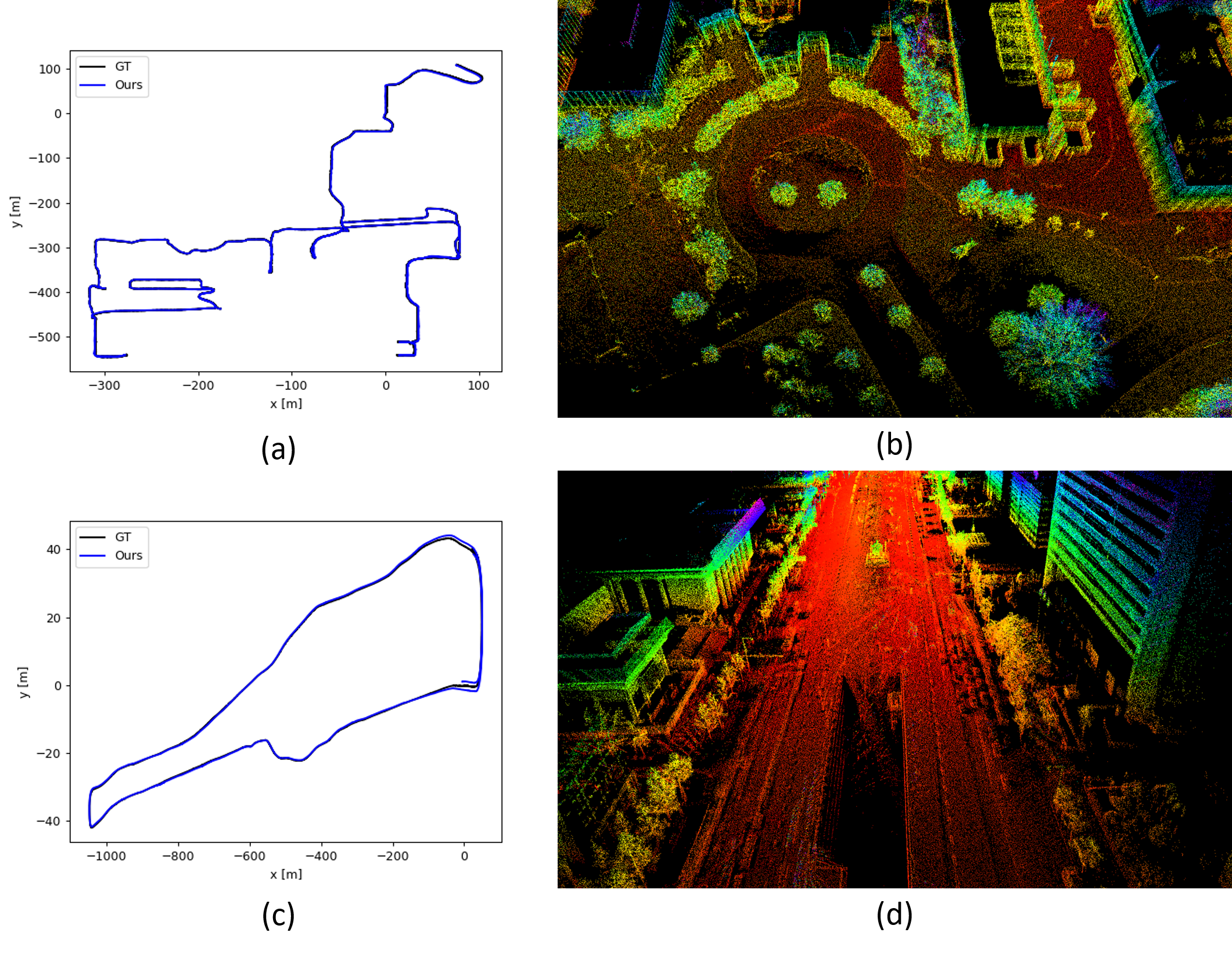
Figure 5: (a) and (c) are the comparison results between our estimated trajectories and ground truth on the exemplar sequences $nclt\_7$ and $kaist\_3$. (b) and (d) are the local point cloud map of $nclt\_7$ and $kaist\_3$ respectively.

We visualize the trajectories and local point cloud maps estimated by our system. The comparison result between our estimated trajectory and ground truth of the exemplar sequences $nclt\_7$ and $kaist\_3$ is shown in Fig. 5 (a) and (c), where our estimated trajectories and ground truth almost exactly coincide. Fig. 5 (b) and (d) show sufficient accuracy for some local structures, where the distribution of the points is also uniform. The demo video of our supplementary material demonstrates that our system can also estimate accurate pose using 16-line Robosense LiDAR.

VII Conclusion

This paper proposes the semi-elastic LiDAR-inertial state estimation method, which can give the state enough flexibility to be optimized to the correct value, thus preferably ensure the accuracy, consistency and robustness of state estimation. We embed the proposed LiDAR-inertial state estimation method into an optimization based LIO framework.

Our system achieves state-of-the-art accuracy and robustness on four public datasets. Meanwhile, the ablation study demonstrates that the proposed semi-elastic LiDAR-inertial method can achieve better consistency for the estimated state.

References

- [1] S. Agarwal, K. Mierle, and T. C. S. Team, “Ceres Solver,” 3 2022. [Online]. Available: https://github.com/ceres-solver/ceres-solver
- [2] J. Behley and C. Stachniss, “Efficient surfel-based slam using 3d laser range data in urban environments.” in Robotics: Science and Systems, vol. 2018, 2018, p. 59.
- [3] J. L. Blanco and P. K. Rai, “nanoflann: a C++ header-only fork of FLANN, a library for nearest neighbor (NN) with kd-trees,” https://github.com/jlblancoc/nanoflann, 2014.
- [4] Y. Cai, W. Xu, and F. Zhang, “ikd-tree: An incremental kd tree for robotic applications,” arXiv preprint arXiv:2102.10808, 2021.
- [5] N. Carlevaris-Bianco, A. K. Ushani, and R. M. Eustice, “University of michigan north campus long-term vision and lidar dataset,” The International Journal of Robotics Research, vol. 35, no. 9, pp. 1023–1035, 2016.
- [6] K. Chen, R. Nemiroff, and B. T. Lopez, “Direct lidar-inertial odometry: Lightweight lio with continuous-time motion correction,” in 2023 IEEE International Conference on Robotics and Automation (ICRA). IEEE, 2023, pp. 3983–3989.
- [7] P. Dellenbach, J.-E. Deschaud, B. Jacquet, and F. Goulette, “Ct-icp: Real-time elastic lidar odometry with loop closure,” in 2022 International Conference on Robotics and Automation (ICRA). IEEE, 2022, pp. 5580–5586.
- [8] J.-E. Deschaud, “Imls-slam: Scan-to-model matching based on 3d data,” in 2018 IEEE International Conference on Robotics and Automation (ICRA). IEEE, 2018, pp. 2480–2485.
- [9] P. Geneva, K. Eckenhoff, W. Lee, Y. Yang, and G. Huang, “Openvins: A research platform for visual-inertial estimation,” in 2020 IEEE International Conference on Robotics and Automation (ICRA). IEEE, 2020, pp. 4666–4672.
- [10] J. Jeong, Y. Cho, Y.-S. Shin, H. Roh, and A. Kim, “Complex urban dataset with multi-level sensors from highly diverse urban environments,” The International Journal of Robotics Research, vol. 38, no. 6, pp. 642–657, 2019.
- [11] K. Li, M. Li, and U. D. Hanebeck, “Towards high-performance solid-state-lidar-inertial odometry and mapping,” IEEE Robotics and Automation Letters, vol. 6, no. 3, pp. 5167–5174, 2021.
- [12] Livox, “Lio-livox: A robust lidar-inertial odometry for livox lidar,” https://github.com/Livox-SDK/LIO-Livox, 2021.
- [13] T. Lupton and S. Sukkarieh, “Visual-inertial-aided navigation for high-dynamic motion in built environments without initial conditions,” IEEE Transactions on Robotics, vol. 28, no. 1, pp. 61–76, 2011.
- [14] C. Qin, H. Ye, C. E. Pranata, J. Han, S. Zhang, and M. Liu, “Lins: A lidar-inertial state estimator for robust and efficient navigation,” in 2020 IEEE international conference on robotics and automation (ICRA). IEEE, 2020, pp. 8899–8906.
- [15] T. Qin, P. Li, and S. Shen, “Vins-mono: A robust and versatile monocular visual-inertial state estimator,” IEEE Transactions on Robotics, vol. 34, no. 4, pp. 1004–1020, 2018.
- [16] T. Shan and B. Englot, “Lego-loam: Lightweight and ground-optimized lidar odometry and mapping on variable terrain,” in 2018 IEEE/RSJ International Conference on Intelligent Robots and Systems (IROS). IEEE, 2018, pp. 4758–4765.
- [17] T. Shan, B. Englot, D. Meyers, W. Wang, C. Ratti, and D. Rus, “Lio-sam: Tightly-coupled lidar inertial odometry via smoothing and mapping,” in 2020 IEEE/RSJ international conference on intelligent robots and systems (IROS). IEEE, 2020, pp. 5135–5142.
- [18] H. W. Sorenson, “Kalman filtering techniques,” in Advances in control systems. Elsevier, 1966, vol. 3, pp. 219–292.
- [19] H. Wang, C. Wang, C.-L. Chen, and L. Xie, “F-loam: Fast lidar odometry and mapping,” in 2021 IEEE/RSJ International Conference on Intelligent Robots and Systems (IROS). IEEE, 2021, pp. 4390–4396.
- [20] H. Wang, C. Wang, and L. Xie, “Intensity scan context: Coding intensity and geometry relations for loop closure detection,” in 2020 IEEE International Conference on Robotics and Automation (ICRA). IEEE, 2020, pp. 2095–2101.
- [21] ——, “Lightweight 3-d localization and mapping for solid-state lidar,” IEEE Robotics and Automation Letters, vol. 6, no. 2, pp. 1801–1807, 2021.
- [22] W. Wen, Y. Zhou, G. Zhang, S. Fahandezh-Saadi, X. Bai, W. Zhan, M. Tomizuka, and L.-T. Hsu, “Urbanloco: A full sensor suite dataset for mapping and localization in urban scenes,” in 2020 IEEE international conference on robotics and automation (ICRA). IEEE, 2020, pp. 2310–2316.
- [23] W. Xu, Y. Cai, D. He, J. Lin, and F. Zhang, “Fast-lio2: Fast direct lidar-inertial odometry,” IEEE Transactions on Robotics, vol. 38, no. 4, pp. 2053–2073, 2022.
- [24] W. Xu and F. Zhang, “Fast-lio: A fast, robust lidar-inertial odometry package by tightly-coupled iterated kalman filter,” IEEE Robotics and Automation Letters, vol. 6, no. 2, pp. 3317–3324, 2021.
- [25] Z. Yan, L. Sun, T. Krajník, and Y. Ruichek, “Eu long-term dataset with multiple sensors for autonomous driving,” in 2020 IEEE/RSJ International Conference on Intelligent Robots and Systems (IROS). IEEE, 2020, pp. 10 697–10 704.
- [26] H. Ye, Y. Chen, and M. Liu, “Tightly coupled 3d lidar inertial odometry and mapping,” in 2019 International Conference on Robotics and Automation (ICRA). IEEE, 2019, pp. 3144–3150.
- [27] Z. Yuan, F. Lang, T. Xu, and X. Yang, “Liw-oam: Lidar-inertial-wheel odometry and mapping,” arXiv preprint arXiv:2302.14298, 2023.
- [28] J. Zhang and S. Singh, “Loam: Lidar odometry and mapping in real-time.” in Robotics: Science and Systems, vol. 2, no. 9. Berkeley, CA, 2014, pp. 1–9.
- [29] ——, “Low-drift and real-time lidar odometry and mapping,” Autonomous Robots, vol. 41, pp. 401–416, 2017.