Joint Adversarial and Collaborative Learning for Self-Supervised Action Recognition

Abstract

Considering the instance-level discriminative ability, contrastive learning methods, including MoCo and SimCLR, have been adapted from the original image representation learning task to solve the self-supervised skeleton-based action recognition task. These methods usually use multiple data streams (i.e., joint, motion, and bone) for ensemble learning, meanwhile, how to construct a discriminative feature space within a single stream and effectively aggregate the information from multiple streams remains an open problem. To this end, we first apply a new contrastive learning method called BYOL to learn from skeleton data and formulate SkeletonBYOL as a simple yet effective baseline for self-supervised skeleton-based action recognition. Inspired by SkeletonBYOL, we further present a joint Adversarial and Collaborative Learning (ACL) framework, which combines Cross-Model Adversarial Learning (CMAL) and Cross-Stream Collaborative Learning (CSCL). Specifically, CMAL learns single-stream representation by cross-model adversarial loss to obtain more discriminative features. To aggregate and interact with multi-stream information, CSCL is designed by generating similarity pseudo label of ensemble learning as supervision and guiding feature generation for individual streams. Exhaustive experiments on three datasets verify the complementary properties between CMAL and CSCL and also verify that our method can perform favorably against state-of-the-art methods using various evaluation protocols. Our code and models are publicly available at https://github.com/Levigty/ACL.

I Introduction

HUMAN action recognition is a fast-developing task due to its wide applications in human-computer interaction, video surveillance, and health care [1, 2, 3]. The underline feature learning algorithms may also benefit image and video applications [4, 5, 6, 7]. Compared with RGB videos or depth data, 3D skeleton data encodes high-level representations of human actions and it is robust to background clutter, illumination changes, and appearance variation [8, 9, 10]. In addition, with the popularity of depth sensors [11] and the development of advanced human pose estimation algorithms [12, 13, 14, 15, 16], the acquisition of skeleton data has become accessible. Thus, skeleton-based action recognition has gradually become a significant branch of action recognition.

Some efforts have been made in previous works. Traditional skeleton-based action recognition methods [17, 18, 19] mainly focus on designing hand-crafted features to model the pattern of the skeleton sequences. With the increasing development of deep learning technologies, Recurrent Neural Networks (RNNs) and Long-Short Term Memory (LSTM) have been exploited to model the temporal dynamics of skeleton sequences [20, 21, 22]. Further, Convolutional Neural Networks (CNNs) based methods [23, 24, 25, 26] propose to convert skeleton sequences to RGB images and then adopt CNNs to learn the discriminative spatio-temporal features. In recent years, due to the similarity between the human skeleton and graph structure, some methods [27, 28, 29] have also been proposed to capture the spatiotemporal relationship based on Graph Convolutional Networks (GCNs), which have achieved superior performances. Nevertheless, the methods mentioned above are all trained in a supervised manner, which requires numerous labeled data to learn the action representation. The cost of labeling large-scale datasets is particularly high. Therefore, self-supervised skeleton-based action recognition has recently received more and more attention [30, 31, 32, 33, 34, 35, 36, 37, 38] due to its ability to better utilize unlabeled data to learn more general feature representations.

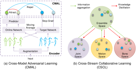
Figure 1: Illustration of our Adversarial and Collaborative Learning (ACL) framework, which mainly involves an Encoder block, a Cross-Model Adversarial Learning (CMAL) block, and a Cross-Stream Collaborative Learning (CSCL) block. (a) For a single stream, better intra-stream representation is learned by CMAL with “Attract” and “Repel” operations on features extracted from an Encoder. (b) For multiple streams, CSAL aggregates inter-stream information and makes the feature space of a single stream to be consistent with the ensemble space. (Best viewed in color)

For self-supervised skeleton-based action recognition, several works [30, 31] design specific generative pretext tasks like reconstruction and prediction to learn representations from unlabeled skeleton sequences. With the development of contrastive self-supervised learning, several works [32, 33, 34] relying on the contrastive learning framework are proposed. They apply data augmentations on the skeleton sequence to construct contrastive pairs (i.e., positive pairs and negative pairs) and hope to learn general representations by pulling the positive pairs closer and pushing the negative pairs away. There are also some methods [35, 36, 37, 38] that combine the generative task with the contrastive task to extract discriminative representations in the multi-task learning manner.

Among them, compared with the generative methods, the contrastive methods pay more attention to the instance-level information rather than the detailed information and then construct a more discriminative feature space that is more suitable for downstream tasks, so it has received extensive attention. Currently, existing contrastive methods for self-supervised skeleton-based action recognition [33, 32, 34] need a careful treatment of negative samples by either relying on large batch sizes, memory banks, or negative sampling strategies to retrieve the negative samples. However, BYOL [39] does not use negative samples, and learns better feature representation through a simple framework, which provides a new idea for the development of contrastive learning in the field of skeleton action recognition. Further, we rethink existing contrastive self-supervised skeleton-based action recognition methods and find several drawbacks. We hope to come up with effective solutions to these problems and then improve the contrastive self-supervised skeleton-based action recognition methods.

1) How to construct a discriminative feature space within a single stream? Although the above methods have improved the skeleton representation ability to a certain extent, it is believed that the ability of self-supervised methods has not been fully explored. Using the BYOL framework [39] directly is not necessarily the most suitable for skeleton action recognition tasks, and the learned feature discrimination could be further improved. Constructing a more discriminative feature space within a single stream is a very challenging problem, especially for the contrastive learning framework without negative samples.

2) How to interact and aggregate the information from multiple streams? In skeleton action recognition, joint, motion, and bone data are three common types of data used to describe human motion. Joint data provides information about the position of each joint in the human body. Motion data describes how the joints are moving over time while bone data describes the spatial relationship between adjacent joints. They are complementary because they each provide unique information and by combining these three types of data, we can get a more complete understanding of the action. However, existing methods often use simple ensemble learning, which cannot perform information interaction well. If such complementary information could be fully utilized and explored, a better feature representation would be obtained. Thus, how to better fuse information between streams needs to be carefully considered.

To this end, we present an Adversarial and Collaborative Learning (ACL) framework to enhance both single-stream and multi-stream representations for self-supervised skeleton-based action recognition. Specifically, SkeletonBYOL is first proposed following BYOL [39] as the baseline. Secondly, Cross-Model Adversarial Learning (CMAL) is proposed to effectively learn single-stream representation as shown in Fig. 1 (a). Unlike BYOL, CMAL is proposed to make the feature “Attract” or “Repel”, and then get a more discriminative feature space. Thirdly, Cross-Stream Collaborative Learning (CSCL) is proposed to aggregate cross-stream information as shown in Fig. 1 (b). The feature distribution of the three streams (i.e., joint, motion, and bone) is fused into an ensemble similarity pseudo-label and the pseudo-label is used as a supervision signal to optimize the feature space of every single stream. Then the pseudo-label continuously updates and iterates to enhance the representations.

In summary, our main contributions are three-fold:

• We present an Adversarial and Collaborative Learning (ACL) framework to effectively enhance both single-stream and multi-stream representations for self-supervised skeleton-based action recognition.

• We formulate a simple yet effective baseline, i.e., SkeletonBYOL. Based on the encoder of SkeletonBYOL, our ACL framework further involves Cross-Model Adversarial Learning (CMAL) and Cross-Stream Collaborative Learning (CSCL) to learn distinctive representations from both single-stream and multi-streams.

• We achieve state-of-the-art performance under a variety of evaluation protocols on three benchmark datasets with observed higher-quality action representations.

The remainder of this paper is organized as follows. We first discuss the related work in Section II. Then we introduce our method in Section III. After that, Section IV provides the experimental results, and Section V concludes this paper.

II Related Work

Supervised Skeleton-based Action Recognition. Traditional skeleton-based action recognition methods [17, 18, 19] mainly design hand-crafted features to represent the skeleton sequences. With the rapid development of deep learning in recent years, some methods [20, 21, 22] use RNNs to model the temporal feature of the skeleton sequence. Since RNNs suffer from gradient vanishing, some methods [23, 24, 40] convert the 3D skeleton sequence into a pseudo image and leverage CNNs to achieve competitive results. However, both RNNs and CNNs fail to fully represent the structure of the skeleton data because the skeleton data are naturally embedded in the form of graphs rather than a vector sequence or 2D matrices. Recently, with the introduction of ST-GCN [27], GCNs have been widely used in the field of skeleton-based action recognition, and a variety of GCN-based methods [28, 29, 41, 42, 43, 44] have emerged on the basis of ST-GCN [27] to better model the spatiotemporal relationship. In this paper, to verify the superiority of our proposed framework, the widely-used ST-GCN is adopted as the encoder to extract features.

Self-supervised Skeleton-based Action Recognition. Self-supervised learning is a specific type of unsupervised learning. It defines specific pretext tasks as the learning targets to learn powerful representations from unlabeled data. For the skeleton sequence data, there are generative pretext tasks [30, 31, 45, 46, 47], contrastive pretext tasks [32, 33, 48, 34, 49, 50, 51, 52], and multiple pretext tasks.

For generative pretext tasks, LongTGAN [30] proposes to use the encoder-decoder to reconstruct the input sequence to obtain useful feature representation. P&C [31] is also based on the reconstruction pretext task, it proposes a training strategy to weaken the decoder, forcing the encoder to learn more discriminative features. Cheng et al. [45] propose to predict the motion of the 3D skeleton as a pretext task and use the Hierarchical Transformer to encode the skeleton sequence. Yang et al. [46] design a novel skeleton cloud colorization technique to learn skeleton representations. Xu et al. [47] propose the Motion Capsule Autoencoder (MCAE) to address the “transformation invariance” challenge in the motion representations. These methods based on frame-level generation are considered not inherently appropriate for representation learning for skeleton-based action recognition [48].

For contrastive pretext tasks, AS-CAL [32] proposes to use plenty of spatiotemporal augmentations and use momentum LSTM and memory bank. SkeletonCLR [33] is built based on MoCo v2 [53, 54] and uses Shear and Crop as the augmentations, which achieves competitive performance. Further, CrosSCLR [33] proposes a cross-view consistent knowledge mining strategy to improve the performance of SkeletonCLR. ST-CL [48] acquires action-specific features by regarding the spatiotemporal continuity of motion tendency as the supervisory signal. Thoker et al. [34] propose inter-skeleton contrastive learning, which learns from multiple different input skeleton representations in a cross-contrastive manner. Xu et al. [49] propose a novel spatiotemporal decouple-and-squeeze contrastive learning (SDS-CL) framework that jointly contrasts spatial-squeezing features, temporal-squeezing features, and global features and use a new attention mechanism to learn better feature. Moliner et al. [50] propose to use vanilla BYOL and asymmetric augmentation, but its gain mainly comes from using a larger number of encoder channels. CMD [51] also uses the MoCo v2 framework and proposes cross-modal mutual distillation to improve the performance. Pang et al. [52] propose a novel contrastive GCN-Transformer network (ConGT), focusing on designing a stronger encoder.

The generative pretext tasks pay more attention to the detailed information of the skeleton sequence, and the contrastive pretext task pays more attention to the discriminative information of the skeleton sequence at the instance level. In order to learn more general features, there are also several methods to do multiple pretext tasks. MS²L [35] proposes to use multiple pretext tasks (i.e., motion prediction, jigsaw puzzle recognition, and contrastive learning) and combine them to encourage the Bi-GRU encoder to capture more suitable features. CP-STN [36] combines contrastive learning paradigms and generative pretext tasks in one framework by using asymmetric spatial and temporal augmentations to enable network-extracting discriminative representations. Tanfous et al. [37] propose to reconcile AS-CAL and P&C by developing a taxonomy of self-supervised learning for action recognition. PCRP [38] proposes a novel framework by prototypical contrast and reverse prediction to fully learn inherent semantic similarity.

Our method belongs to the category of using contrastive pretext tasks. Different from the existing methods[33, 32, 48], our method focuses on exploring a new baseline to obtain more discriminative features within a single stream and focuses on how to interact and aggregate information between different streams to obtain a more discriminative feature space than ensemble learning. The proposed method has a simpler structure and is applicable to a variety of encoders.

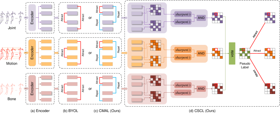
Figure 2: Comparison between our proposed Adversarial and Collaborative Learning (ACL) framework and our proposed simple baseline, i.e., SkeletonBYOL. Our ACL framework consists of (a) Encoder, (c) CMAL, and (d) CSCL. Meanwhile, the SkeletonBYOL consists of (a) Encoder and (b) BYOL. Noting that the Encoder contains Augmentation, Online Network, and Target Network. (Best viewed in color)

III Method

III-A SkeletonBYOL

Contrastive learning has been widely used due to its instance discrimination capability. Inspired by this, we develop SkeletonBYOL to learn single-stream 3D action representations based on the recent advanced practice, i.e., Bootstrap Your Own Latent (BYOL) [39]. It is a non-negative samples method for skeleton representation, which only considers one sample’s different augments as its positive samples. In each training step, the positive samples are embedded close to each other. SkeletonBYOL consists of four major components.

Augmentation. Data augmentations $\mathcal{T}$ are used to randomly transform the given skeleton sequence $s$ into different augments $x$ and $x^{\prime}$ that are considered as positive pairs. For skeleton data, Shear and Crop are adopted as the augmentation strategy following SkeletonCLR [33].

(i) Shear: The shear augmentation is a linear transformation in the spatial dimension. The shape of 3D coordinates of body joints is slanted with a random angle. The transformation matrix is defined as:

$$A=\left[\begin{array}[]{ccc}1&a_{12}&a_{13}\\ a_{21}&1&a_{23}\\ a_{31}&a_{32}&1\end{array}\right],$$ (1)

where $a_{12}$, $a_{13}$, $a_{21}$, $a_{23}$, $a_{31}$, $a_{32}$ are shear factors that randomly sampled from a uniform distribution $[-\beta,\beta]$, where $\beta$ is the shear amplitude. Following SkeletonCLR, $\beta=0.5$, then the skeleton sequence is multiplied by the transformation matrix $A$ on the channel dimension.

(ii) Crop: For image classification, crop is a commonly used data augmentation, because it can increase the diversity while maintaining the distinction of original samples. For the temporal skeleton sequence, specifically, we symmetrically pad some frames to the sequence and then randomly crop it to the original length. The padding length is defined as $T/\gamma$, where $\gamma$ is the padding ratio, and here we set $\gamma=6$.

Online Network. The online network is defined by a set of weights $\theta$ and is comprised of three components: an encoder $f_{\theta}$, a projector $g_{\theta}$, and a predictor $q_{\theta}$. The encoder $f_{\theta}$ embeds $x$ into feature space: $y_{\theta}={f_{\theta}}(x)$. The projector $g_{\theta}$ is a multi-layer perceptron (MLP), which consists of a linear layer followed by batch normalization, a rectified linear unit (ReLU), and a final linear layer. $g_{\theta}$ is used to project the feature vector to a new feature space: $z_{\theta}={g_{\theta}}({y_{\theta}})$. The predictor $q_{\theta}$ is used to predict the output of the target network, which has the same structure as $g_{\theta}$. The parameters $\theta$ of the online network are updated via gradients.

Target Network. The target network is comprised of two components: an encoder $f_{\xi}$ and a projector $g_{\xi}$. They have the same architecture as that in online network but use a different set of weights $\xi$. The target network provides the regression targets to train the online network: $y^{\prime}_{\xi}={f_{\xi}}(x^{\prime})$, $z^{\prime}_{\xi}={g_{\xi}}({y^{\prime}_{\xi}})$. Its parameters $\xi$ are an exponential moving average of the online parameters $\theta$. More precisely, given a target decay rate $\tau\in\left[{0,1}\right]$, after each training step we perform the update:

$${\xi}\leftarrow\tau{\xi}+(1-\tau){\theta}.$$ (2)

BYOL. Finally we define the following mean squared error between the $l_{2}$-normalized prediction ${q_{\theta}}({z_{\theta}})$ and target projections ${{z^{\prime}}_{\xi}}$:

$$\mathcal{L}_{\theta,\xi} =\left\|{{q_{\theta}}({z_{\theta}})-sg({{z^{\prime}}_{\xi}})}\right\|_{2}^{2}$$ (3)

$$=2-2\cdot\frac{{\left\langle{{q_{\theta}}({z_{\theta}}),sg({{z^{\prime}}_{\xi}})}\right\rangle}}{{{{\left\|{{q_{\theta}}({z_{\theta}})}\right\|}_{2}}\cdot{{\left\|{sg({{z^{\prime}}_{\xi}})}\right\|}_{2}}}},$$

where $\left\langle,\right\rangle$ denotes the inner product and $sg(\cdot)$ means stop-gradient. We symmetrize the loss $\mathcal{L}_{\theta,\xi}$ in Eq. (3) by feeding $x^{\prime}$ to the online network and $x$ to the target network to compute $\tilde{\mathcal{L}}_{\theta,\xi}$. At each training step, a stochastic optimization step is performed to minimize $\mathcal{L}_{BYOL}=\mathcal{L}_{\theta,\xi}+\tilde{\mathcal{L}}_{\theta,\xi}$.

Algorithm 1  Pseudocode of the Encoder and CMAL

$\mathcal{D}$ is a training set

$\mathcal{L}_{total}$ is the loss value

1:$\mathcal{L}_{total}\leftarrow 0$

2:for a minibatch $s$ in $\mathcal{D}$ with $n$ samples do

3:     get the augmented sample $x$ and $x^{\prime}$

4:     use the online network to obtain the online feature $z_{\theta}$ and $z_{\theta}^{\prime}$ $\leftarrow x,x^{\prime}$

5:     use the online predictor to obtain the predicted feature $p_{\theta}$ and $p_{\theta}^{\prime}$ $\leftarrow z_{\theta},z_{\theta}^{\prime}$

6:     use the target network to obtain the online feature $z_{\xi}$ and $z_{\xi}^{\prime}$ $\leftarrow x,x^{\prime}$

7:     use the mean square error to obtain the loss value in a mini-batch:

8:$\mathcal{L}_{CMAL}=mse(p_{\theta},p_{\theta}^{\prime})-\frac{1}{2}(mse(p_{\theta},z_{\xi})+mse(p_{\theta}^{\prime},z_{\xi}^{\prime}))$

9:     loss backward

10:     update the online network with gradient

11:     update the target network with momentum update

12:     $\mathcal{L}_{total}\leftarrow\mathcal{L}_{total}+\mathcal{L}_{CMAL}$

13:end for

14:return $\mathcal{L}_{total}$

III-B CMAL

SkeletonBYOL predicts the output of the target network from an online network. It discards the negative samples completely and achieves good performance. However, it is difficult to understand intuitively why this direct prediction is valid. It is difficult to obtain a more discriminative feature space. Inspired by RAFT [55], we hope to better use the framework and optimize two goals at the same time: (i) keeping representations of two augmented samples of the same action sequence aligned and (ii) keeping a sample’s online representation differing from its target representation. Thus, CMAL is proposed to learn single-stream representation more effectively.

For an input sequence $s$, features $z_{\theta}$, $z^{\prime}_{\theta}$, $z_{\xi}$ and $z^{\prime}_{\xi}$ are extracted. Then prediction head is used to obtain $q_{\theta}(z_{\theta})$ and $q_{\theta}(z^{\prime}_{\theta})$. In order to obtain a more discriminative feature space and avoid collapse solutions, we first hope to align representations of $x$ and $x^{\prime}$ similar by ${\mathcal{L}}_{min}$:

$$\mathcal{L}_{min}=\left\|{{q_{\theta}}({z_{\theta}})-{q_{\theta}}({{z^{\prime}}_{\theta}})}\right\|_{2}^{2}.$$ (4)

On the other hand, we also hope the feature of the online encoder could be different from the target encoder by ${\mathcal{L}}_{max}$ to obtain a more discriminative feature space:

$$\begin{split}\mathcal{L}_{max}=-\frac{1}{2}&\left(\left\|{{q_{\theta}}({z_{\theta}})-sg({z_{\xi}})}\right\|_{2}^{2}\right.\\ &+\left.\left\|{{q_{\theta}}({{z^{\prime}}_{\theta}})-sg({{z^{\prime}}_{\xi}})}\right\|_{2}^{2}\right).\end{split}$$ (5)

To joint optimize these two goals, our final cross-model adversarial loss is as follows: $\mathcal{L}_{CMAL}=\alpha{\mathcal{L}_{min}}+\beta{\mathcal{L}_{max}}$, where $\alpha$ and $\beta$ are the coefficients to balance the loss. The two models are updated through momentum, but at the same time, the extracted features are expected to maximize the similarity as much as possible, which forms an implicit confrontation, effectively avoiding model collapse and constructing a more discriminative feature space. The pseudocode of using both the Encoder and the CMAL is in Algorithm 1.

III-C CSCL

Considering easily-obtained multi-stream skeleton data (i.e., joint, motion, and bone), fusing complementary information preserved in different streams can definitely learn better spatiotemporal information. We design CSCL to mine more ideal feature space in multiple streams.

(i) Intra-stream similarity. In single-stream, we gather ${q_{\theta}}({z_{\theta}})$, ${q_{\theta}}({z^{\prime}_{\theta}})$, $sg({z_{\xi}})$, $sg({z^{\prime}_{\xi}})$ in a batch and do L2-normalization to get ${Q,Q^{\prime},K,K^{\prime}}\in\mathbb{R}^{N\times C}$, respectively. $N$ represents the batch size and $C$ represents the feature dimension. As shown in Fig. 3 (a), we first calculate the cosine similarity in a mini-batch for a single stream. Take “joint stream” as an example:

$${\mathcal{S}_{joint}}=QK^{\prime\top},{\mathcal{S^{\prime}}_{joint}}=Q^{\prime}K^{\top},$$ (6)

where ${\mathcal{S}_{joint}},{\mathcal{S^{\prime}}_{joint}}\in\mathbb{R}^{N\times N}$. Correspondingly, the similarity matrix $\mathcal{S}_{bone}$, $\mathcal{S}^{\prime}_{bone}$ of bone stream and $\mathcal{S}_{motion}$, $\mathcal{S}^{\prime}_{motion}$ of motion stream can also be obtained in a similar way.

(ii) Intra-stream fusion. We hope to get a sharper similarity matrix to obtain a more discriminative feature space. As shown in Fig. 3 (b), we use $sharpen(\cdot)$ to make the similarity matrix sharp in a single stream:

$${\hat{\mathcal{S}}_{J}}=sharpen({\mathcal{S}}_{joint})\;{\rm AND}\;sharpen({\mathcal{S}}^{\prime}_{joint}),$$ (7)

here, $sharpen(\cdot)$ operation means setting the diagonal elements and the top-$k$ elements of each row of the similarity matrix to $1$, and the others to $0$ to obtain a sharper similarity matrix. Then perform an “AND” operation to obtain the similarity pseudo-label within the stream. In a similar way, we can get ${\hat{\mathcal{S}}_{B}}$ and ${\hat{\mathcal{S}}_{M}}$, respectively.

(iii) Inter-stream voting. In Fig. 3 (c), we propose to fuse the similarity matrix of three streams to obtain a more ideal similarity matrix ${\hat{\mathcal{S}}}=vote({\hat{\mathcal{S}}_{J}},{\hat{\mathcal{S}}_{B}},{\hat{\mathcal{S}}_{M}})$, where $vote(\cdot)$ means ensembling the results to determine the value of each element is $1$ or $0$. Specifically, when there are more than two streams that think the element should be 1, it will be 1, otherwise, it will be 0. Undoubtedly, the result of ensemble learning is better than that of a single stream, so the sharper similarity matrix ${\hat{\mathcal{S}}}$ is more discriminative than ${\hat{\mathcal{S}}_{J}}$, ${\hat{\mathcal{S}}_{B}}$, and ${\hat{\mathcal{S}}_{M}}$.

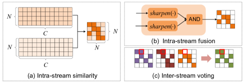
Figure 3: Three key components of our proposed CSCL. (Best viewed in color)

(iv) Optimization goal. A very intuitive idea is to use ${\hat{\mathcal{S}}}$ as a supervision signal to optimize the similarity matrix of each stream, then the optimized similarity matrix of each stream can better generate ${\hat{\mathcal{S}}}$. In this way, information between different streams can be effectively aggregated, thereby obtaining better feature representations. Thus, the similarity difference minimization loss can be calculated like this:

$${{\cal L}_{CSCL}}=-\frac{1}{2}\sum\limits{\left[{\hat{\mathcal{S}}\log({{\mathcal{S}}_{i}})+(1-\hat{\mathcal{S}})\log(1-{{\mathcal{S}}_{i}})}\right]},$$ (8)

where ${\mathcal{S}}_{i}\in\{{\mathcal{S}_{joint}},{\mathcal{S^{\prime}}_{joint}},{\mathcal{S}_{motion}},{\mathcal{S^{\prime}}_{motion}},{\mathcal{S}_{bone}},{\mathcal{S^{\prime}}_{bone}}\}$. This loss is expected to make the feature similarity of every single stream approach the feature similarity of the ensemble feature. Minimizing the difference in similarity rather than minimizing the difference in features is a softer way to obtain a better feature space.

Training. In the early training stage, the encoder of each stream is not stable and strong enough to perform cross-stream information aggregation. Thus, for the ACL framework, the Encoder is trained with the Cross-Model Adversarial Loss: ${\cal L}_{1}={\cal L}_{CMAL}$ in the first training stage. Then in the second training stage, the loss function is ${\cal L}_{2}=\lambda{{\cal L}_{CMAL}}+\gamma{{\cal L}_{CSCL}}$ to start aggregating cross-stream information. Here, $\lambda$ and $\gamma$ are the coefficients to balance the loss.

IV Experiments

IV-A Datasets

PKU-MMD Dataset [56] consists of two subsets that contain almost 20,000 action sequences covering 51 action classes. Part I is an easier version for action recognition, while part II is more challenging due to the large view variation causing more skeleton noise. We conduct experiments under the cross-subject protocol on the two subsets.

NTU-60 Dataset [57] contains 56,578 action sequences and 60 action classes. There are two evaluation protocols: cross-subject (xsub) and cross-view (xview). In xsub, half of the subjects are used as training sets, and the rest are used as test sets. In xview, the sequences of camera 2 and 3 are used for training while the sequences of camera 1 are used for testing.

NTU-120 Dataset [58] contains 120 action classes and 113,945 sequences. There are also two evaluation protocols: cross-subject (xsub) and cross-setup (xset). In xsub, actions performed by 53 subjects are for training and the others are for testing. In xset, all 32 setups are separated as half for training and the other half for testing.

IV-B Experimental Settings

TABLE I: Comparison under KNN evaluation protocol with joint stream.

Method	PKU-MMD(%)		NTU-60(%)		NTU-120(%)
	part I	part II	xsub	xview	xsub	xset
SkeletonCLR [33]	65.9	17.9	57.7	67.3	44.9	45.8
CMAL (Ours)	77.1	36.6	64.2	72.3	50.0	52.1

TABLE II: Linear evaluation results on three datasets.

Method	Encoder	Classifier	NTU-60(%)		NTU-120(%)		PKU-MMD(%)		Publication&Year
			xsub	xview	xsub	xset	part I	part II
LongTGAN [30]	GRU	FC	39.1	48.1	-	-	67.7†	26.0†	AAAI’2018
MS2L [35]	GRU	GRU	52.6	-	-	-	64.9	27.6	ACMMM’2020
P&C [31]	GRU	FC	50.7	61.1	41.7	42.7	-	-	CVPR’2020
PCRP [38]	GRU	FC	53.9	63.5	41.7	45.1	-	-	TMM’2021
AS-CAL [32]	LSTM	FC	58.5	64.8	48.6	49.2	-	-	Infomation Science’2021
ACL (Ours)	GRU	FC	63.7	69.0	54.6	55.0	84.0	39.9	-
4s-MG-AL [59]	ST-GCN	FC	64.7	68.0	46.2	49.5	-	-	TCSVT’2022
Cheng et al. [45]	Transformer	FC	69.3	72.8	-	-	-	-	ICME’2021
MCAE [47]	MCAE	FC	65.6	74.7	52.8	54.7	-	-	NIPS’2021
CP-STN [36]	ST-GCN	FC	69.4	76.6	55.7	54.7	-	-	ACML’2021
ST-CL [48]	GCN	FC	68.1	69.4	54.2	55.6	-	-	TMM’2022
SDS-CL [49]	DSTA	FC	73.6	78.9	50.6	55.6	-	-	TNNLS’2023
3s-CrosSCLR [33]	ST-GCN	FC	77.8	83.4	67.9	66.7	84.9†	21.2†	CVPR’2021
Yang et al. [46]	DGCNN	FC	75.2	83.1	-	-	-	-	ICCV’2021
Thoker et al. [34]	GRU+CNN	FC	76.3	85.2	67.1	67.9	80.9	36.0	ACMMM’2020
3s-AimCLR [60]	ST-GCN	FC	78.9	83.8	68.2	68.8	87.8	38.5	AAAI’2022
ACL (Ours)	ST-GCN	FC	78.6	84.5	68.5	71.1	88.1	53.4	-

• ^† denotes the result is reproduced according to the provided code.

TABLE III: Semi-supervised evaluation results.

Method	PKU-MMD(%)		NTU-60(%)
	part I	part II	xsub	xview
1% labeled data:
LongT GAN [30]	35.8	12.4	35.2	-
MS2L [35]	36.4	13.0	33.1	-
ISC [34]	37.7	-	35.7	38.1
3s-Colorization [46]	-	-	48.3	52.5
3s-CrosSCLR [33]	49.7	10.2	51.1	50.0
ACL (Ours)	58.7	17.7	51.1	49.7
10% labeled data:
LongT GAN [30]	69.5	25.7	62.0	-
MS2L [35]	70.3	26.1	65.2	-
ISC [34]	72.1	-	65.9	72.5
3s-Colorization [46]	-	-	71.7	78.9
3s-CrosSCLR [33]	82.9	28.6	74.4	77.8
ACL (Ours)	86.7	37.2	76.2	79.6

TABLE IV: Finetuned results on NTU-60 and NTU-120 dataset.

Method	NTU-60(%)		NTU-120(%)
	xsub	xview	xsub	xset
ST-GCN [27]	82.8	91.0	76.4	76.8
CMAL (Ours)	83.9	91.6	77.4	79.4
3s-ST-GCN [27]	85.1	91.8	80.0	80.4
3s-CrosSCLR [33]	86.2	92.5	80.5	80.4
3s-AimCLR [60]	86.9	92.8	80.1	80.9
ACL (Ours)	86.9	92.8	81.7	82.7

TABLE V: Exploration of different pretext datasets for fine-tuning on PKU-MMD dataset.

Pretext Task Dataset	PKU-MMD(%)
	part I	part II
w/o pretext task	92.3	53.7
PKU-MMD	94.1 (+1.8)	58.5 (+4.8)
NTU-60 xsub	95.1 (+2.8)	61.2 (+7.5)
NTU-120 xsub	94.7 (+2.4)	62.4 (+8.7)

TABLE VI: Ablation study results on NTU-60 dataset.

Method	NTU-60(%)
	xsub	xview
SkeletonCLR [33]	75.0	79.8
SkeletonBYOL (Baseline: Encoder + BYOL)	77.3	82.6
CMAL (Encoder + CMAL)	78.0	83.6
CSCL (Encoder + CSCL)	78.5	84.2
ACL (Encoder + CMAL + CSCL)	78.6	84.5

TABLE VII: Linear evaluation results compared with SkeletonCLR on NTU-60, PKU-MMD, and NTU-120 datasets.

Method	Stream	NTU-60(%)				PKU-MMD(%)				NTU-120(%)
		xsub		xview		part I		part II		xsub		xset
		acc.	$\Delta$	acc.	$\Delta$	acc.	$\Delta$	acc.	$\Delta$	acc.	$\Delta$	acc.	$\Delta$
SkeletonCLR [33]	J	68.3		76.4		80.9		35.2		56.8		55.9
CMAL (Ours)	J	73.0	$\uparrow$ 4.7	79.4	$\uparrow$ 3.0	86.3	$\uparrow$ 5.4	47.7	$\uparrow$ 12.5	61.6	$\uparrow$ 4.8	63.2	$\uparrow$ 7.3
SkeletonCLR [33]	M	53.3		50.8		63.4		13.5		39.6		40.2
CMAL (Ours)	M	57.7	$\uparrow$ 4.4	62.4	$\uparrow$ 11.6	72.1	$\uparrow$ 8.7	29.1	$\uparrow$ 15.6	43.5	$\uparrow$ 3.9	46.2	$\uparrow$ 6.0
SkeletonCLR [33]	B	69.4		67.4		72.6		30.4		48.4		52.0
CMAL (Ours)	B	70.0	$\uparrow$ 0.6	74.0	$\uparrow$ 6.6	83.3	$\uparrow$ 10.7	34.1	$\uparrow$ 3.7	59.2	$\uparrow$ 10.8	59.2	$\uparrow$ 7.2
3s-SkeletonCLR [33]	J+M+B	75.0		79.8		85.3		40.4		60.7		62.6
CMAL (Ours)	J+M+B	78.0	$\uparrow$ 3.0	83.6	$\uparrow$ 3.8	87.4	$\uparrow$ 2.1	52.8	$\uparrow$ 12.4	66.8	$\uparrow$ 6.1	70.0	$\uparrow$ 7.4
3s-CrosSCLR [33]	J+M+B	77.8		83.4		84.9		21.2		67.9		66.7
ACL (Ours)	J+M+B	78.6	$\uparrow$ 0.8	84.5	$\uparrow$ 0.9	88.1	$\uparrow$ 3.2	53.4	$\uparrow$ 32.2	68.5	$\uparrow$ 0.6	71.1	$\uparrow$ 4.4

• $\Delta$ represents the gain compared to SkeletonCLR using the same stream data. J, M and B indicate joint stream, motion stream, bone stream, respectively. 3s means using three stream.

Pretext Training. All experiments are conducted on the PyTorch framework [61] with a single GeForce GTX 3090 GPU. For data pre-processing, mini-batch size, and encoder, we all follow CrosSCLR [33] for fair comparisons. The representation $y_{\theta}$ has a feature dimension of 512. The projection head consists of a linear layer with output size 2048 followed by batch normalization, a rectified linear unit (ReLU), and a final linear layer with output dimension 512. The architecture of the prediction head is the same as the projection head. The target decay rate $\tau$ is set to 0.996. For optimization, we use SGD with momentum (0.9), weight decay (0.0001), and a learning rate of 0.1. Since the size of the three datasets varies greatly, it is favourable to set different training epochs for them to avoid overfitting and achieve better convergence. For NTU-60, we set the training epoch to 100 (the first 60 epoch is the first training stage). For NTU-120, we set the training epoch to 80 (the first 40 epoch is the first training stage). For PKU-MMD Part I, we set the training epoch to 150 (the first 100 epoch is the first training stage). For PKU-MMD Part II, we set the training epoch to 250 (the first 200 epoch is the first training stage).

Downstream Testing. We evaluate the trained encoder under multiple protocols after the pretext training.

(i) KNN Evaluation Protocol. A K-Nearest Neighbor (KNN) classifier is used on the features of the trained encoder. It can reflect the quality of the features learned by the encoder. For all reported KNN results, $K=20$.

(ii) Linear Evaluation Protocol. The encoder is verified by linear evaluation for the action recognition task. To train a classification head, we fix the encoder and use an SGD with an initial learning rate of 3.0 to train the classification head (a fully connected layer followed by a softmax layer) for 100 epochs. The learning rate decreases to 0.3 at epoch 80. The batch size is set to 128.

(iii) Semi-supervised Evaluation Protocol. We append a linear classifier to the trained encoder and then train the whole model with only 1% or 10% randomly selected labeled data. An SGD with an initial learning rate of 0.1 (decreases by 10 at epoch 80) is used. The whole network is also trained for 150 epochs with batch size set to 128, except for PKU-MMD part II under 1% semi-supervised evaluation protocol (set to 52 due to the limited data).

(iv) Finetune Evaluation Protocol. We append a linear classifier to the trained encoder and then train the whole model with all labeled data to compare it with end-to-end training methods. An SGD with an initial learning rate of 0.1 (decreases to 0.01 at epoch 80) is used to train the network for 150 epochs. The batch size is set to 128.

TABLE VIII: Results of different stream on NTU-60 dataset.

Method	Stream	xsub(%)	xview(%)
CMAL	J	73.0	79.4
CMAL	M	58.8	62.9
CMAL	B	70.1	74.0
CMAL ‡	J + B	74.8	80.5
CMAL ‡	J + M	74.5	79.3
CMAL ‡	M + B	73.3	78.1
CMAL ‡	J + M + B	76.2	81.4
ACL	J + B	77.8	83.1
ACL	J + M	75.4	83.9
ACL	M + B	76.4	81.7
ACL	J + M + B	78.6	84.5

• ${\ddagger}$ represents directly ensemble the results.

IV-C Comparison with State-of-the-Art Methods

KNN Evaluation Results. Compared with the linear classifier, the KNN classifier does not require learning extra weights. The results in Table I are fair comparisons under the sample value of $K$, and we can see that our single-stream CMAL is better than SkeletonCLR [33] on the three datasets under the KNN classifier. The obvious gains of using a simple classifier also show that the features learned by our CMAL are more discriminative.

Linear Evaluation Results. As shown in Table II, we compare the proposed ACL with other recent methods. For using GRU as the encoder, our ACL outperforms other methods on the three datasets under the linear evaluation protocol. For using stronger encoders, our ACL also leads 3s-AimCLR under many protocols. For the performance on NTU-120, our ACL still outperforms other methods by a large margin. This shows that our ACL is very competitive on multi-class large-scale datasets. For PKU-MMD dataset, Part II is more challenging with more skeleton noise caused by the view variation. Notably, 3s-CrosSCLR suffers on part II while our ACL performs very well. It also proves that our methods have a strong ability to cope with movement patterns caused by skeleton noise. Based on the above, our ACL performs well on both large-scale and small-scale datasets, which demonstrates the effectiveness and generalization of our method.

Semi-Supervised Evaluation Results. With only 1% or 10% labeled data, the spatial-temporal representations learned by the encoder in pretext task are important because the small amount of data can lead to difficult convergence or overfitting problems. From Table III, even only with a small labeled subset, our ACL performs better than other methods. The results of using 1% and 10% labeled data exceed ISC [34], 3s-CrosSCLR [27], and 3s-Colorization [46]. It also proves that our method effectively learns intra-inter stream information and obtains a more discriminative feature space.

Finetuned Evaluation Results. We compare our method with supervised ST-GCN and supervised 3s-ST-GCN, which have the same structure and parameters as ours. As shown in Table IV, our CMAL achieves better results than supervised ST-GCN, which means that our framework could learn more information to get a better weight initialization. For the results of three streams, the finetuned results also outperform supervised 3s-ST-GCN and finetuned 3s-CrosSCLR, which indicates the effectiveness of our method.

Transfer Learning Results. As a common practice, transfer learning performs self-supervised pre-training on the large-scale ImageNet [62], then initialize the network with the learned weights and finally train on the small dataset. We also conduct experiments to do pretext tasks on a larger dataset without labels, then finetune on the small dataset. In Table V, when training from scratch, the accuracy of part I and part II is 92.3% and 53.7%. When we do the pretext task on the PKU-MMD dataset itself, we can gain the improvement of 1.8% and 4.8%. When applying the NTU-60 and NTU-120 datasets for self-supervised pre-training, we can significantly improve the accuracy by a large margin in part II, which illustrates the benefits of the transferability of learned representation.

IV-D Ablation Study

TABLE IX: Feature dimension search experiments on joint stream of NTU-60 dataset.

$d_{y}$	$h_{mlp}$	$d_{z}$	xsub(%)	xview(%)	Avg.(%)
256	1024	256	69.4	74.0	71.7
256	1024	512	69.4	74.3	71.9
256	1024	1024	69.7	73.7	71.7
512	1024	256	70.8	76.9	73.9
512	1024	512	72.7	75.4	74.1
512	1024	1024	71.0	77.0	74.0
512	512	512	71.3	76.7	74.0
512	2048	512	73.2	78.2	75.7

TABLE X: Results of different target decay rate $\tau$. (%)

$\tau$	xsub	xview	Avg.
1	54.7	58.6	56.7
0.999	70.8	76.1	73.4
0.996	73.0	79.4	76.2
0.99	73.2	78.2	75.7
0.9	68.9	74.0	71.5
0	55.2	54.8	55.0

TABLE XI: Results of different Top-$K$ in ISIA on NTU-60 dataset. (%)

Top-$K$	xsub	xview
$0$	78.0	83.6
$1$	78.7	84.4
$2$	78.6	84.5
$3$	78.3	83.9
$4$	77.6	83.4
$5$	76.6	78.5

TABLE XII: Results of different weights to balance $\mathcal{L}_{min}$ and $\mathcal{L}_{max}$. (%)

$\alpha$	$\beta$	xsub	xview
$1$	$0$	8.0	7.9
$0$	$1$	31.9	40.4
$1$	$0.1$	60.3	68.6
$1$	$1$	73.0	79.4
$1$	$10$	62.1	60.3

TABLE XIII: Results of different weights to balance ${\cal L}_{CMAL}$ and ${\cal L}_{CSCL}$. (%)

$\lambda$	$\gamma$	xsub	xview
$1$	$0$	78.0	83.5
$0$	$1$	77.4	82.3
$1$	$0.1$	77.2	81.5
$1$	$1$	64.1	53.6
$1$	$10$	78.6	84.5

TABLE XIV: Results of our CMAL on NTU-60 joint stream with different backbone.

Backbone	Setting	NTU-60(%)
		xsub	xview
ST-GCN	Supervised	82.8	91.0
	Finetuned	83.9	91.6
CTR-GCN	Supervised	84.0	91.2
	Finetuned	85.5	91.7
UNIK	Supervised	83.2	89.8
	Finetuned	84.4	91.6

Effectiveness of CMAL and CSCL. We also verify the effectiveness of our proposed individual components. In Table VI, SkeletonCLR [33] achieves 75.0% on xsub and 79.8% on xview while the proposed SkeletonBYOL achieves 77.3% on xsub and 82.6% on xview. Our CMAL outperforms these results by 0.7% and 1.0%. For the proposed CSCL, applying it to the Encoder also brings significant gains, which also shows the effectiveness of the strategy. For our complete method ACL, it achieves 78.6% and 84.5%.

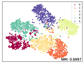
(a) SkeletonCLR [33]

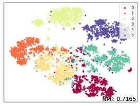
(b) SkeletonBYOL (Ours)

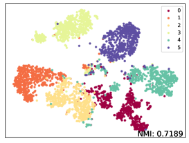
(c) CMAL (Ours)

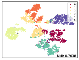
(d) 3s-CrosSCLR [33]

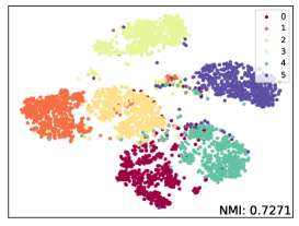
(e) 3s-CMAL (Ours)

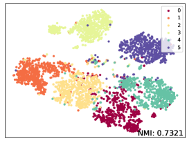
(f) ACL (Ours)

Figure 4: The t-SNE visualization of embeddings on NTU-60 xview. Different methods extract features for 6 categories of samples, and the visualization results after feature dimensionality reduction are shown in the figure. Noting that 3s-CMAL means using CMAL on three streams.

Comparisons with SkeletonCLR. We compare our CMAL with the SkeletonCLR in more detail. As shown in Table VII, for the three different streams (i.e., joint, motion, and bone) of three datasets, our CMAL outperforms SkeletonCLR. For the direct ensemble results, our CMAL also outperforms 3s-SkeletonCLR. It is worth mentioning that both 3s-CrosSCLR and our ACL explore the information interaction between streams, but our method outperforms 3s-CrosSCLR on three datasets on account that our method better aggregates information from multiple streams.

Choice of Feature Dimension. Since the predictor has the same structure as the projector, there are three hyper-parameters of feature dimension: the dimension of feature $y$ after encoder $d_{y}$, the dimension of projector’s hidden layer $h_{mlp}$ and the dimension of projector’s final layer $d_{z}$. To determine them, we first fix $h_{mlp}$ and find that the performance of $d_{y}=512$ is better than that of $d_{y}=256$ as shown in Table IX. Then we fix $d_{z}$ to search for the best $h_{mlp}$. Based on the results, we choose $d_{y}=512$, $h_{mlp}=2048$, $d_{z}=512$ as our default settings.

Influence of Target Decay Rate $\tau$. The value of $\tau$ is a trade-off between updating the target network too often and updating too slowly in Table XI. When $\tau=1$, the target network is never updated and remains at a constant value corresponding to its initialization. When $\tau=0$, the target network is instantaneously updated to the online network at each step. Both $\tau=0$ and $\tau=1$ destabilize training, yielding very poor performance. The values of the decay rate between 0.9 and 0.999 yield better performance and we choose $\tau=0.996$.

Influence of Top-$K$. From Table XI, $K=0$ means that do not use the ISIA. It is worth mentioning that ISIA brings clear gains when $0<K<4$. This is because the $Sharpen(\cdot)$ and inter-stream voting retain high confidence samples to learn better feature representations. When $K$ continues to increase, it has a bad impact on performance due to the introduction of too many low-confidence samples. Finally, we take $K$ to 2 according to performance.

Influence of Weights in $\mathcal{L}_{CMAL}$. We also conducted experiments to verify the performance of different weights in $\mathcal{L}_{CMAL}$. In Table XIII, using only $\mathcal{L}_{min}$ ($\alpha=1$, $\beta=0$) or $\mathcal{L}_{max}$ ($\alpha=0$, $\beta=1$) does not perform well. The best performance is achieved when $\mathcal{L}_{min}$ and $\mathcal{L}_{max}$ are equally important ($\alpha=1$, $\beta=1$), which is also in line with our original intention when designing cross-model adversarial loss.

Influence of Weights to Balance ${\cal L}_{CMAL}$ and ${\cal L}_{CSCL}$. As shown in Table XIII, when do not use the ${\cal L}_{CSCL}$ ($\lambda=1$, $\gamma=0$), the performance is also good. However, there is a drop in performance when only using ${\cal L}_{CSCL}$ ($\lambda=0$, $\gamma=1$), but not that noticeable. Interestingly, the performance degrades when the weights of ${\cal L}_{CMAL}$ and ${\cal L}_{CSCL}$ are the same. Moreover, for our ACL, $\lambda=1$ and $\gamma=10$ are the best choice. We argue that it is because information aggregation is more important in the second stage of training.

Robustness to Different Backbones. ST-GCN [27] is widely used as a backbone in the field of skeleton-based action recognition. To verify the robustness of our method to different backbones, we explore the performance of our method when using a more advanced backbone. We tried CTR-GCN [63] (GCN-based) and UNIK [64] (CNN-based). Due to the limitation of computing resources, for fair comparisons, like ST-GCN, the input frames of CTR-GCN and UNIK are also 50 frames, and the number of channels in the network is also reduced to 1/4 of the original. Due to these changes, the fully supervised results drop somewhat compared to the results in the original paper. But thankfully, as shown in Table XIV, under the same experimental setting, our method can improve the performance of end-to-end training. This also illustrates the potential and generalizability of our method to different backbones.

Qualitative Results. We apply t-SNE [65] with fix settings to show the embedding distribution in Fig. 4. The reported t-SNE results are fair comparisons with the same randomly selected 6 class samples. From the visual results and the calculated NMI (Normalized Mutual Information), we can draw a conclusion that our SkeletonBYOL and CMAL could cluster the embeddings of the same class closer than SkeletonCLR. For multi-streams, even without CA, our 3s-CMAL achieves a more competitive NMI compared to the 3s-CrosSCLR (0.7271 vs 0.7038). Our final ACL achieves the best NMI.

V Conclusion

This paper focuses on self-supervised representation learning in skeleton-based action recognition and design an ACL framework to enhance intra-inter stream representations from unlabeled data. The SkeletonBYOL based on the BYOL framework is first constructed. On this basis, CMAL is proposed to leverage cross-model adversarial loss to learn intra-stream representation more effectively. For multi-streams, CSCL is proposed to aggregate inter-stream information to further enhance the representations. Experiments show that our proposed ACL framework performs favorably against state-of-the-art methods under a variety of evaluation protocols.

References

- [1] Z. Tu, H. Li, D. Zhang, J. Dauwels, B. Li, and J. Yuan, “Action-stage emphasized spatiotemporal vlad for video action recognition,” IEEE Transactions on Image Processing (TIP), vol. 28, no. 6, pp. 2799–2812, 2019.
- [2] M. Liu, F. Meng, and Y. Liang, “Generalized pose decoupled network for unsupervised 3d skeleton sequence-based action representation learning,” Cyborg and Bionic Systems (CBS), vol. 2022, p. 0002, 2022.
- [3] J. Zhang, Y. Jia, W. Xie, and Z. Tu, “Zoom transformer for skeleton-based group activity recognition,” IEEE Transactions on Circuits and Systems for Video Technology (TCSVT), vol. 32, no. 12, pp. 8646–8659, 2022.
- [4] F.-L. Zhang, M.-M. Cheng, J. Jia, and S.-M. Hu, “Imageadmixture: Putting together dissimilar objects from groups,” IEEE Transactions on Visualization and Computer Graphics (TVCG), vol. 18, no. 11, pp. 1849–1857, 2012.
- [5] H.-C. Liu, F.-L. Zhang, D. Marshall, L. Shi, and S.-M. Hu, “High-speed video generation with an event camera,” The Visual Computer (TVC), vol. 33, pp. 749–759, 2017.
- [6] Z.-H. Zheng, H.-T. Zhang, F.-L. Zhang, and T.-J. Mu, “Image-based clothes changing system,” Computational Visual Media (CVM), vol. 3, pp. 337–347, 2017.
- [7] F.-L. Zhang, X. Wu, R.-L. Li, J. Wang, Z.-H. Zheng, and S.-M. Hu, “Detecting and removing visual distractors for video aesthetic enhancement,” IEEE Transactions on Multimedia (TMM), vol. 20, no. 8, pp. 1987–1999, 2018.
- [8] Z. Tu, J. Zhang, H. Li, Y. Chen, and J. Yuan, “Joint-bone fusion graph convolutional network for semi-supervised skeleton action recognition,” IEEE Transactions on Multimedia (TMM), 2022.
- [9] M. Liu, F. Meng, C. Chen, and S. Wu, “Novel motion patterns matter for practical skeleton-based action recognition,” in AAAI Conference on Artificial Intelligence (AAAI), 2023.
- [10] J. Liu, X. Wang, C. Wang, Y. Gao, and M. Liu, “Temporal decoupling graph convolutional network for skeleton-based gesture recognition,” IEEE Transactions on Multimedia (TMM), 2023.
- [11] Z. Zhang, “Microsoft kinect sensor and its effect,” IEEE Multimedia, vol. 19, no. 2, pp. 4–10, 2012.
- [12] Z. Cao, G. Hidalgo, T. Simon, S.-E. Wei, and Y. Sheikh, “OpenPose: Realtime multi-person 2D pose estimation using part affinity fields,” IEEE Transactions on Pattern Analysis and Machine Intelligence (TPAMI), vol. 43, no. 1, pp. 172–186, 2019.
- [13] H.-S. Fang, S. Xie, Y.-W. Tai, and C. Lu, “RMPE: Regional multi-person pose estimation,” in Proceedings of the IEEE International Conference on Computer Vision (ICCV), 2017, pp. 2334–2343.
- [14] J. Martinez, R. Hossain, J. Romero, and J. J. Little, “A simple yet effective baseline for 3D human pose estimation,” in Proceedings of the IEEE International Conference on Computer Vision (ICCV), 2017, pp. 2640–2649.
- [15] D. Pavllo, C. Feichtenhofer, D. Grangier, and M. Auli, “3D human pose estimation in video with temporal convolutions and semi-supervised training,” in Proceedings of the IEEE Conference on Computer Vision and Pattern Recognition (CVPR), 2019, pp. 7753–7762.
- [16] W. Li, H. Liu, R. Ding, M. Liu, P. Wang, and W. Yang, “Exploiting temporal contexts with strided transformer for 3D human pose estimation,” IEEE Transactions on Multimedia, 2022.
- [17] J. Wang, Z. Liu, Y. Wu, and J. Yuan, “Mining actionlet ensemble for action recognition with depth cameras,” in Proceedings of the IEEE Conference on Computer Vision and Pattern Recognition (CVPR), 2012, pp. 1290–1297.
- [18] R. Vemulapalli, F. Arrate, and R. Chellappa, “Human action recognition by representing 3D skeletons as points in a lie group,” in Proceedings of the IEEE Conference on Computer Vision and Pattern Recognition (CVPR), 2014, pp. 588–595.
- [19] R. Vemulapalli and R. Chellapa, “Rolling rotations for recognizing human actions from 3D skeletal data,” in Proceedings of the IEEE Conference on Computer Vision and Pattern Recognition (CVPR), 2016, pp. 4471–4479.
- [20] Y. Du, W. Wang, and L. Wang, “Hierarchical recurrent neural network for skeleton based action recognition,” in Proceedings of the IEEE Conference on Computer Vision and Pattern Recognition (CVPR), 2015, pp. 1110–1118.
- [21] S. Song, C. Lan, J. Xing, W. Zeng, and J. Liu, “Spatio-temporal attention-based LSTM networks for 3D action recognition and detection,” IEEE Transactions on Image Processing (TIP), vol. 27, no. 7, pp. 3459–3471, 2018.
- [22] P. Zhang, C. Lan, J. Xing, W. Zeng, J. Xue, and N. Zheng, “View adaptive neural networks for high performance skeleton-based human action recognition,” IEEE Transactions on Pattern Analysis and Machine Intelligence (TPAMI), vol. 41, no. 8, pp. 1963–1978, 2019.
- [23] Y. Du, Y. Fu, and L. Wang, “Skeleton based action recognition with convolutional neural network,” in Proceedings of the Asian Conference on Pattern Recognition (ACPR), 2015, pp. 579–583.
- [24] Q. Ke, M. Bennamoun, S. An, F. Sohel, and F. Boussaid, “A new representation of skeleton sequences for 3D action recognition,” in Proceedings of the IEEE Conference on Computer Vision and Pattern Recognition (CVPR), 2017, pp. 3288–3297.
- [25] C. Cao, C. Lan, Y. Zhang, W. Zeng, H. Lu, and Y. Zhang, “Skeleton-based action recognition with gated convolutional neural networks,” IEEE Transactions on Circuits and Systems for Video Technology (TCSVT), vol. 29, no. 11, pp. 3247–3257, 2018.
- [26] A. Banerjee, P. K. Singh, and R. Sarkar, “Fuzzy integral-based CNN classifier fusion for 3D skeleton action recognition,” IEEE Transactions on Circuits and Systems for Video Technology (TCSVT), vol. 31, no. 6, pp. 2206–2216, 2020.
- [27] S. Yan, Y. Xiong, and D. Lin, “Spatial temporal graph convolutional networks for skeleton-based action recognition,” in Proceedings of the AAAI Conference on Artificial Intelligence (AAAI), vol. 32, no. 1, 2018.
- [28] L. Shi, Y. Zhang, J. Cheng, and H. Lu, “Two-stream adaptive graph convolutional networks for skeleton-based action recognition,” in Proceedings of the IEEE Conference on Computer Vision and Pattern Recognition (CVPR), 2019, pp. 12 026–12 035.
- [29] Z. Chen, S. Li, B. Yang, Q. Li, and H. Liu, “Multi-scale spatial temporal graph convolutional network for skeleton-based action recognition,” in Proceedings of the AAAI Conference on Artificial Intelligence (AAAI), vol. 35, no. 2, 2021, pp. 1113–1122.
- [30] N. Zheng, J. Wen, R. Liu, L. Long, J. Dai, and Z. Gong, “Unsupervised representation learning with long-term dynamics for skeleton based action recognition,” in Proceedings of the AAAI Conference on Artificial Intelligence (AAAI), vol. 32, no. 1, 2018.
- [31] K. Su, X. Liu, and E. Shlizerman, “Predict & Cluster: Unsupervised skeleton based action recognition,” in Proceedings of the IEEE Conference on Computer Vision and Pattern Recognition (CVPR), 2020, pp. 9631–9640.
- [32] H. Rao, S. Xu, X. Hu, J. Cheng, and B. Hu, “Augmented skeleton based contrastive action learning with momentum LSTM for unsupervised action recognition,” Information Sciences, vol. 569, pp. 90–109, 2021.
- [33] L. Li, M. Wang, B. Ni, H. Wang, J. Yang, and W. Zhang, “3D human action representation learning via cross-view consistency pursuit,” in Proceedings of the IEEE Conference on Computer Vision and Pattern Recognition (CVPR), 2021, pp. 4741–4750.
- [34] F. M. Thoker, H. Doughty, and C. G. Snoek, “Skeleton-contrastive 3D action representation learning,” in ACM International Conference on Multimedia (ACMMM), 2021, pp. 1655–1663.
- [35] L. Lin, S. Song, W. Yang, and J. Liu, “MS2L: Multi-task self-supervised learning for skeleton based action recognition,” in Proceedings of the ACM International Conference on Multimedia (ACM MM), 2020, pp. 2490–2498.
- [36] Y. Zhan, Y. Chen, P. Ren, H. Sun, J. Wang, Q. Qi, and J. Liao, “Spatial temporal enhanced contrastive and pretext learning for skeleton-based action representation,” in Asian Conference on Machine Learning (ACML), 2021, pp. 534–547.
- [37] A. B. Tanfous, A. Zerroug, D. Linsley, and T. Serre, “How and what to learn: Taxonomizing self-supervised learning for 3D action recognition,” in IEEE Winter Conference on Applications of Computer Vision (WACV), 2022, pp. 2888–2897.
- [38] S. Xu, H. Rao, X. Hu, J. Cheng, and B. Hu, “Prototypical contrast and reverse prediction: Unsupervised skeleton based action recognition,” IEEE Transactions on Multimedia (TMM), 2021.
- [39] J.-B. Grill, F. Strub, F. Altché, C. Tallec, P. Richemond, E. Buchatskaya, C. Doersch, B. Avila Pires, Z. Guo, M. Gheshlaghi Azar et al., “Bootstrap your own latent-a new approach to self-supervised learning,” Proceedings of the Advances in Neural Information Processing Systems (NeurIPS), vol. 33, pp. 21 271–21 284, 2020.
- [40] M. Liu, H. Liu, and C. Chen, “Enhanced skeleton visualization for view invariant human action recognition,” Pattern Recognition, vol. 68, pp. 346–362, 2017.
- [41] H. Zheng and X. Zhang, “A cross view learning approach for skeleton-based action recognition,” IEEE Transactions on Circuits and Systems for Video Technology (TCSVT), 2021.
- [42] J. Kong, H. Deng, and M. Jiang, “Symmetrical enhanced fusion network for skeleton-based action recognition,” IEEE Transactions on Circuits and Systems for Video Technology (TCSVT), vol. 31, no. 11, pp. 4394–4408, 2021.
- [43] S. Miao, Y. Hou, Z. Gao, M. Xu, and W. Li, “A central difference graph convolutional operator for skeleton-based action recognition,” IEEE Transactions on Circuits and Systems for Video Technology (TCSVT), 2021.
- [44] C. Wu, X.-J. Wu, and J. Kittler, “Graph2net: Perceptually-enriched graph learning for skeleton-based action recognition,” IEEE Transactions on Circuits and Systems for Video Technology (TCSVT), 2021.
- [45] Y.-B. Cheng, X. Chen, J. Chen, P. Wei, D. Zhang, and L. Lin, “Hierarchical transformer: Unsupervised representation learning for skeleton-based human action recognition,” in IEEE International Conference on Multimedia and Expo (ICME), 2021, pp. 1–6.
- [46] S. Yang, J. Liu, S. Lu, M. H. Er, and A. C. Kot, “Skeleton cloud colorization for unsupervised 3D action representation learning,” in Proceedings of the IEEE International Conference on Computer Vision (ICCV), 2021.
- [47] Z. Xu, X. Shen, Y. Wong, and M. S. Kankanhalli, “Unsupervised motion representation learning with capsule autoencoders,” Advances in Neural Information Processing Systems (NeurIPS), vol. 34, 2021.
- [48] X. Gao, Y. Yang, Y. Zhang, M. Li, J.-G. Yu, and S. Du, “Efficient spatio-temporal contrastive learning for skeleton-based 3D action recognition,” IEEE Transactions on Multimedia (TMM), 2021.
- [49] B. Xu, X. Shu, J. Zhang, G. Dai, and Y. Song, “Spatiotemporal decouple-and-squeeze contrastive learning for semi-supervised skeleton-based action recognition,” IEEE Transactions on Neural Networks and Learning Systems (TNNLS), 2023.
- [50] O. Moliner, S. Huang, and K. Åström, “Bootstrapped representation learning for skeleton-based action recognition,” in Proceedings of the IEEE Conference on Computer Vision and Pattern Recognition Workshop (CVPRW), 2022, pp. 4154–4164.
- [51] Y. Mao, W. Zhou, Z. Lu, J. Deng, and H. Li, “CMD: Self-supervised 3D action representation learning with cross-modal mutual distillation,” in Proceedings of the European Conference on Computer Vision (ECCV), 2022, pp. 734–752.
- [52] C. Pang, X. Lu, and L. Lyu, “Skeleton-based action recognition through contrasting two-stream spatial-temporal networks,” IEEE Transactions on Multimedia (TMM), 2023.
- [53] K. He, H. Fan, Y. Wu, S. Xie, and R. Girshick, “Momentum contrast for unsupervised visual representation learning,” in Proceedings of the IEEE Conference on Computer Vision and Pattern Recognition (CVPR), 2020, pp. 9729–9738.
- [54] X. Chen, H. Fan, R. Girshick, and K. He, “Improved baselines with momentum contrastive learning,” arXiv preprint arXiv:2003.04297, 2020.
- [55] H. Shi, D. Luo, S. Tang, J. Wang, and Y. Zhuang, “Run away from your teacher: Understanding BYOL by a novel self-supervised approach,” arXiv preprint arXiv:2011.10944, 2020.
- [56] J. Liu, S. Song, C. Liu, Y. Li, and Y. Hu, “A benchmark dataset and comparison study for multi-modal human action analytics,” ACM Transactions on Multimedia Computing, Communications, and Applications, vol. 16, no. 2, pp. 1–24, 2020.
- [57] A. Shahroudy, J. Liu, T.-T. Ng, and G. Wang, “NTU RGB + D: A large scale dataset for 3D human activity analysis,” in Proceedings of the IEEE Conference on Computer Vision and Pattern Recognition (CVPR), 2016, pp. 1010–1019.
- [58] J. Liu, A. Shahroudy, M. Perez, G. Wang, L.-Y. Duan, and A. C. Kot, “NTU RGB + D 120: A large-scale benchmark for 3D human activity understanding,” IEEE Transactions on Pattern Analysis and Machine Intelligence (TPAMI), vol. 42, no. 10, pp. 2684–2701, 2019.
- [59] Y. Yang, G. Liu, and X. Gao, “Motion guided attention learning for self-supervised 3D human action recognition,” IEEE Transactions on Circuits and Systems for Video Technology (TCSVT), 2022.
- [60] T. Guo, H. Liu, Z. Chen, M. Liu, T. Wang, and R. Ding, “Contrastive learning from extremely augmented skeleton sequences for self-supervised action recognition,” in Proceedings of the AAAI Conference on Artificial Intelligence (AAAI), vol. 36, no. 1, 2022, pp. 762–770.
- [61] A. Paszke, S. Gross, F. Massa, A. Lerer, J. Bradbury, G. Chanan, T. Killeen, Z. Lin, N. Gimelshein, L. Antiga et al., “Pytorch: An imperative style, high-performance deep learning library,” Proceedings of the Advances in Neural Information Processing Systems (NeurIPS), vol. 32, pp. 8026–8037, 2019.
- [62] O. Russakovsky, J. Deng, H. Su, J. Krause, S. Satheesh, S. Ma, Z. Huang, A. Karpathy, A. Khosla, M. Bernstein et al., “Imagenet large scale visual recognition challenge,” International Journal of Computer Vision (IJCV), vol. 115, no. 3, pp. 211–252, 2015.
- [63] Y. Chen, Z. Zhang, C. Yuan, B. Li, Y. Deng, and W. Hu, “Channel-wise topology refinement graph convolution for skeleton-based action recognition,” in IEEE International Conference on Computer Vision (ICCV), 2021, pp. 13 359–13 368.
- [64] D. Yang, Y. Wang, A. Dantcheva, L. Garattoni, G. Francesca, and F. Bremond, “UNIK: A unified framework for real-world skeleton-based action recognition,” arXiv preprint arXiv:2107.08580, 2021.
- [65] L. Van der Maaten and G. Hinton, “Visualizing data using t-sne,” Journal of Machine Learning Research, vol. 9, no. 11, 2008.