Reducing operator complexity in Algebraic Multigrid with Machine Learning Approaches

Abstract

We propose a data-driven and machine-learning-based approach to compute non-Galerkin coarse-grid operators in algebraic multigrid (AMG) methods, addressing the well-known issue of increasing operator complexity. Guided by the AMG theory on spectrally equivalent coarse-grid operators, we have developed novel ML algorithms that utilize neural networks (NNs) combined with smooth test vectors from multigrid eigenvalue problems. The proposed method demonstrates promise in reducing the complexity of coarse-grid operators while maintaining overall AMG convergence for solving parametric partial differential equation (PDE) problems. Numerical experiments on anisotropic rotated Laplacian and linear elasticity problems are provided to showcase the performance and compare with existing methods for computing non-Galerkin coarse-grid operators.

65M55, 65F08, 65F10, 15A60

1 Introduction

Algebraic Multigrid (AMG) methods are one of the most efficient and scalable iterative methods for solving linear systems of equations

(1) $$Au=f$$

where the coefficient matrix $A\in\mathbb{R}^{N\times N}$ is sparse and large, and $u\in\mathbb{R}^{N}$ and $f\in\mathbb{R}^{N}$ are the solution and right-hand-side vectors respectively. For the systems that arise from elliptic-type partial differential equations (PDEs), AMG methods often exhibit optimal linear computational complexities. Nevertheless, there is ongoing research focused on further improving the efficiency and scalability of AMG methods, in particular for large-scale and challenging problems. By and large, the overall efficiency of iterative methods is determined by not only the convergence rate of the iterations but also the arithmetic complexity per iteration and the corresponding throughput on the underlying computing platform. In this work, we address a common issue in AMG methods that is the growth of the coarse-grid operator complexity in the hierarchy. This operator is typically computed as the Galerkin product from the operators in the fine level. Assuming $A$ is symmetric positive definite (SPD), the Galerkin operator is optimal in the sense that it yields an orthogonal projector as the coarse-grid correction that guarantees to reduce the $A$-norm of the error. However, on the other hand, this operator can lead to the issue of increasing operator sparsity, particularly at deeper levels of the AMG hierarchy. This can impair the overall performance of AMG by introducing challenges in terms of computational efficiency, memory requirements, and the communication cost in distributed computing environments. Moreover, the increasing operator complexity can also affect the effectiveness and robustness of other AMG components such as the coarsening and interpolation algorithms. To demonstrate this problem, we consider classical AMG methods for solving the 3-D Poisson’s equation discretized on a $100\times 100\times 100$ grid with a 7-point stencil. The sparsity patterns of the operator matrix $A^{(l)}$ at the levels $l=0,3,5$ are shown in Fig. 1. From these patterns, it is evident that the matrix bandwidth increases as the level goes deeper, as well as the stencil size (i.e., the average number of nonzeros per row). The increased sparsity often leads to not only a growth in computational cost but also an increase in data movement, which corresponds to the communication expense in parallel solvers. Fig. 2 shows the time spent in the computation and communication in the first 6 levels of the AMG hierarchies for solving this 3-D Poisson’s problem. As depicted, there is a steep increase in the computational cost at level 2, coinciding with the level where the communication cost reaches its maximum.

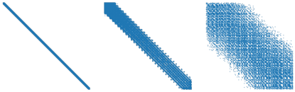
level	N	NNZ	RNZ
0	1,000,000	6,940,000	7
1	500,000	8,379,408	17
2	128,630	5,814,096	45
3	23,023	1,727,541	75
4	11,688	1,371,218	117

Figure 1: The sparsity patterns of $A^{(0)}$, $A^{(3)}$, and $A^{(5)}$ in the AMG hierarchy for solving the 3-D Poisson’s equation (top). The size of the operator matrix (N), the number of nonzeros (NNZ) and the average number of nonzeros per row (RNZ) across the AMG levels (bottom).

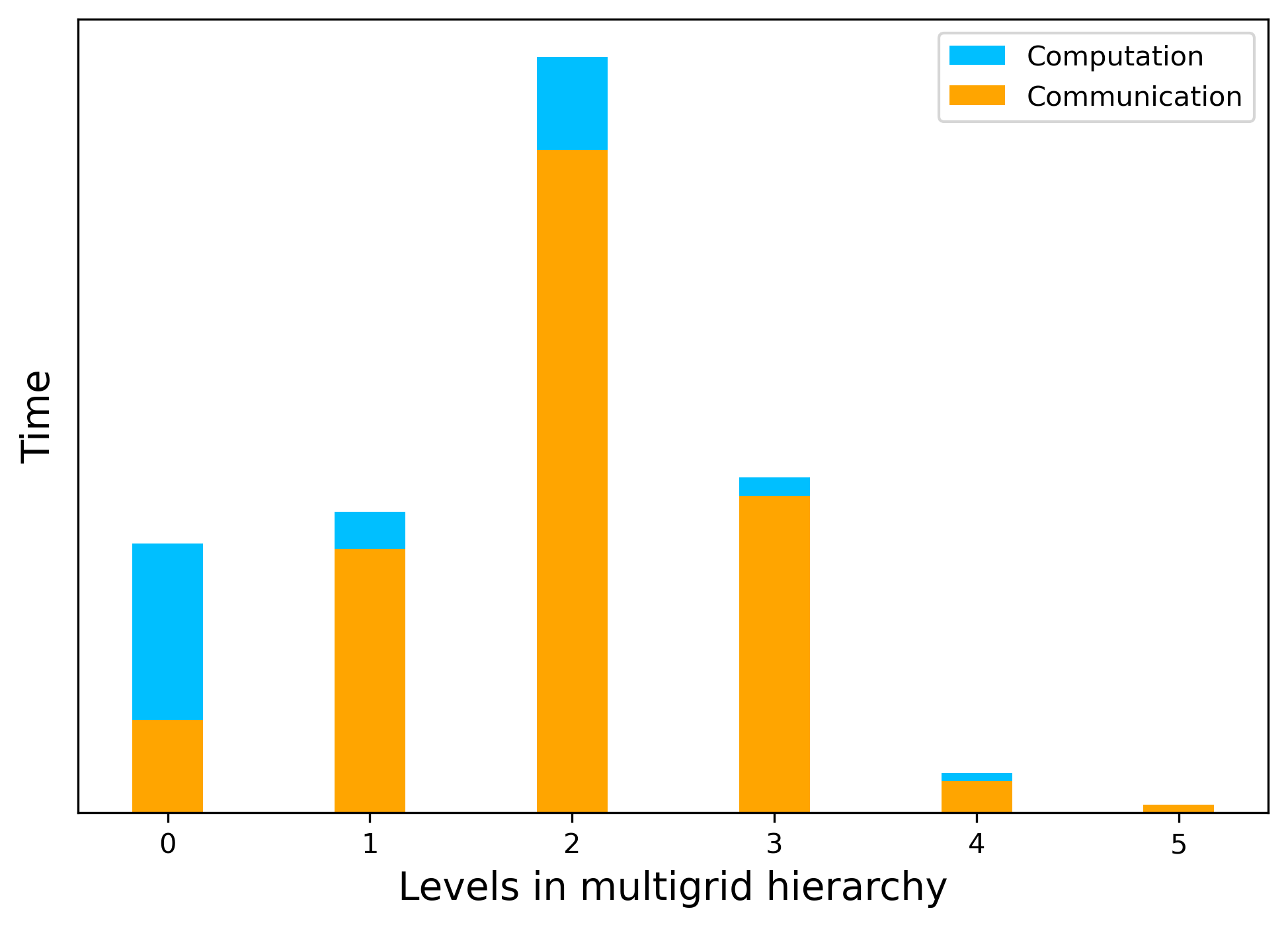
Figure 2: The cost of computation and communication in the first 6 levels of parallel AMG methods for solving the 3-D Poisson’s equation. Image source: [4]

One approach to reducing the coarse-grid operator complexity is to “sparsify” the Galerkin operator after it is computed, i.e., removing some nonzeros outside a given sparsity pattern. The obtained sparsified operator is often called a “non-Galerkin” coarse-grid operator. The methods developed in [30, 28] leverage algebraically smooth basis vectors and the approximations to the fine grid operator to explicitly control the coarse grid sparsity pattern. The algorithms introduced in [10, 27] first determine the patterns of the sparsified operator based on heuristics on the path of edges in the corresponding graph and then compute the numerical values to ensure the spectral equivalence to the Galerkin operator for certain types of PDEs. Improving the parallel efficiency of AMG by reducing the communication cost with the non-Galerkin operator was discussed in [3]. These existing algorithms for computing non-Galerkin operators are usually based on heuristics on the associated graph and the characteristic of the underlying PDE problem, such as the information of the near kernels of $A$. Therefore, they are problem-dependent, and often times it can be difficult to devise such heuristics that are suitable for a broader class of problems.

Recently, there has been a line of work in the literature to leverage data-driven and ML-based methods to improve the robustness of AMG. In particular, [23, 21, 11] deal with learning better prolongation operators. Techniques of deep reinforcement learning (DRL) are exploited in [26] to better tackle the problem of AMG coarsening combined with the diagonal dominance ratio of the F-F block. Both the works in [19] and [22] focus on the problem of designing better smoothers. In [19], smoothers are directly parameterized by multi-layer convolution neural networks (CNNs) while [22] optimizes the weights in the weighted Jacobi smoothers. In this paper, we follow this line of research and propose a data-driven and ML-based method for non-Galerkin operators. The innovations and features of the proposed method are summarized as follows: 1) Introduction of a multi-level algorithm based on ML methods to sparsify all coarse-grid operators in the AMG hierarchy; 2) Successful reduction of operator density while preserving the convergence behavior of the employed AMG method; 3) Applicability of the proposed NN model to a class of parametric PDEs with parameters following specific probability distributions; 4) Ability to train the sparsified coarse-grid operator on each level in parallel once the training data is prepared; 5) Flexibility for the user to choose the average number of non-zero entries per row in the coarse-grid operators, with a minimum threshold requirement. To the best of our knowledge, our proposed work is the first to utilize ML models for controlling sparsity within the hierarchy of AMG levels.

The rest of the paper is organized as follows. We first briefly review the preliminaries of AMG methods and the non-Galerkin algorithms in Section 2. We elaborate on our proposed sparsification algorithm in Section 3. Numerical experiments and results are presented in Section 4. Finally, we conclude in Section 5.

2 AMG preliminaries and coarse-grid operators

In this section, we give a brief introduction to AMG methods and the Galerkin coarse-grid operators. The AMG method is a multilevel method that utilizes a hierarchy of grids, consisting of fine and coarse levels, and constructs coarse-level systems at different scales that can capture the essential information of the fine-level system while reducing the problem size. AMG algorithms employ techniques such as coarsening, relaxation, restriction and interpolation to transfer information between the grid levels to accelerate the solution process. Algorithm 1 presents the most commonly used AMG V-cycle scheme. It uses $\nu$ steps of pre- and post-smoothing, where $M$ and $M^{\mathsf{T}}$ are the smoothing operators. Matrices $R$ and $P$ are the restriction and prolongation operators, respectively. The coarse-grid operator is computed in Step 3 via the Galerkin product, $A_{g}=RAP$. The aim of the smoothings is to quickly annihilate the high-frequency errors via simple iterative methods such as relaxation, whereas the low-frequency errors are targeted by the Coarse-Grid Correction (CGC) operator, $I-P(RAP)^{-1}RA$. When $R=P^{\mathsf{T}}$, the CGC operator is $A$-orthogonal with the Galerkin operator $A_{g}$.

Algorithm 1 Multigrid V-Cycle for solving $A^{(l)}u^{(l)}=f^{(l)}$ at level $l$

1:  Pre-smoothing: $u^{(l)}:=(I-(M^{(l)})^{-1}A^{(l)})u^{(l)}+(M^{(l)})^{-1}f^{(l)}$ for $\nu$ steps

2:  Compute residual $r^{(l)}=f^{(l)}-A^{(l)}u^{(l)}$ and the restriction $r^{(l+1)}=R^{(l)}r^{(l)}$

3:  Compute Galerkin operator $A_{g}=R^{(l)}A^{(l)}P^{(l)}$ and let $A^{(l+1)}=A_{g}$

4:  if $l=L-1$ then

5:     Solve $A^{(l+1)}u^{(l+1)}=r^{(l+1)}$ with an arbitrary method

6:  else

7:     Let $u^{(l+1)}=0$ and $f^{(l+1)}=r^{(l+1)}$. Go to Step 1 with $l:=l+1$.

8:  end if

9:  Prolongate and correct: $u^{(l)}:=u^{(l)}+P^{(l)}u^{(l+1)}$

10:  Post-smoothings: $u^{(l)}:=(I-(M^{(l)})^{-\mathsf{T}}A^{(l)})u^{(l)}+(M^{(l)})^{-\mathsf{T}}f^{(l)}$ for $\nu$ steps

2.1 Non-Galerkin operators

Naive approaches, such as indiscriminately removing nonzero entries in the Galerkin operators based on the magnitude often result in slow convergence of the overall AMG method (see the example provided in Section 3 of [10]). To address the aforementioned challenges arising from the increased operator complexity in the Galerkin operator $A_{g}$, alternative operators, denoted by $A_{c}$, that are not only sparser than $A_{g}$ but also spectrally equivalent have been studied and used in lieu of the Galerkin operator.

Definition 2.1.

SPD matrices $A_{g}$ and $A_{c}$ are spectrally equivalent if

(2) $$0<\alpha\leq\lambda(A_{g}^{-1}A_{c})\leq\beta,$$

with $\alpha$ and $\beta$ both close to 1.

The convergence rate of AMG can be analyzed through the spectral radius of the error propagation matrix. For example, the two-grid error propagation matrix corresponding to the V-cycle in Algorithm 1 reads

(3) $$E_{g}=(I-M^{-\mathsf{T}}A)^{\nu}(I-PA_{g}^{-1}RA)(I-M^{-1}A)^{\nu}.$$

With the replacement of $A_{g}$ by $A_{c}$, it becomes

(4) $$E_{c}=(I-M^{-\mathsf{T}}A)^{\nu}(I-PA_{c}^{-1}RA)(I-M^{-1}A)^{\nu}.$$

The spectrum property of $E_{c}$ is analyzed in the following theorem.

Theorem 2.2 ([10]).

Denoting by $B_{g}$ and $B_{c}$ respectively the corresponding preconditioning matrices induced by $E_{g}=I-B_{g}^{-1}A$ and $E_{c}=I-B_{c}^{-1}A$, and assuming $A_{c}$ and $A_{g}$ are both SPD and

(5) $$\theta=\|I-A_{c}A_{g}^{-1}\|_{2}=\|I-A_{g}^{-1}A_{c}\|_{2}<1,$$

for the preconditioned matrix, we have

(6) $$\kappa(B^{-1}_{c}A)\leq\frac{1+\theta}{1-\theta}\kappa(B^{-1}_{g}A),$$

and moreover

(7) $$\rho(E_{c})\leq\max\left(\frac{\lambda_{\max}(B^{-1}_{g}A)}{1-\theta}-1,1-\frac{\lambda_{\min}(B_{g}^{-1}A)}{1+\theta}\right),$$

where $\lambda_{\mathrm{max}}(\cdot)$ and $\lambda_{\mathrm{min}}(\cdot)$ are the largest and smallest eigenvalues respectively, $\kappa(\cdot)$ denotes the condition number and $\rho(\cdot)$ denotes the spectrum radius.

The quantity $\theta$ measures the degree of spectral equivalence between the operators $A_{g}$ and $A_{c}$, i.e., only when $\theta$ is small, these operators are spectrally equivalent. Clearly, the condition number of the preconditioned matrix and the two-grid convergence with respect to $E_{c}$ deteriorate as $\theta$ increases. With fixed $B_{g}^{-1}A$, we can establish a criterion for the convergence of $E_{c}$ with respect to $\theta$, as shown in the next result.

Corollary 2.3.

Suppose $\theta<1-\lambda_{\max}(B_{g}^{-1}A)/2$, the two-grid method Eq. 4 converges.

Proof 2.4.

Note that $\theta<1-\lambda_{\max}(B_{g}^{-1}A)/{2}$ implies that ${\lambda_{\max}(B_{g}^{-1}A)}/{(1-\theta)}-1<1$. Since $\lambda(B_{g}^{-1}A)>0$, $1-\lambda_{\min}(B_{g}^{-1}A)/{(1+\theta)}<1$. Therefore, from (7), it follows that $\rho(E_{c})<1$.

2.2 Spectrally equivalent stencils

In this paper, we focus on structured matrices that can be represented by stencils and grids. These structured matrices exhibit a unique property wherein two spectrally equivalent stencils can determine two sequences of spectrally equivalent matrices with increasing sizes and thus ensures the convergence of $E_{c}$ with increasing matrix sizes.

Definition 2.5 ([1, 5]).

Let $\{A_{j}\}$ and $\{B_{j}\}$ be two sequences of (positive definite) matrices with increasing size $N_{j}$, where $A_{j}$ and $B_{j}\in\mathbb{R}^{N_{j}\times N_{j}}$. If $A_{j}$ and $B_{j}$ are spectrally equivalent as defined in Eq. 2 for all $j$ with $\alpha$ and $\beta$ that are independent of $N_{j}$, then the sequences $\{A_{j}\}$ and $\{B_{j}\}$ are called spectrally equivalent sequences of matrices.

The above definition yields the definition of spectrally equivalent stencils.

Definition 2.6 ([5]).

Suppose the sequences of matrices $\{A_{j}\}$ and $\{B_{j}\}$ are constructed with the stencils $\mathcal{A}$ and $\mathcal{B}$ respectively, where $A_{j}$ and $B_{j}$ have the same size for all $j$. We call $\mathcal{A}$ and $\mathcal{B}$ are spectrally equivalent if $\{A_{j}\}$ and $\{B_{j}\}$ are spectrally equivalent sequences of matrices.

At the end of this section, we provide an example of spectrally equivalent stencils. Consider the following 9-point stencil that was used in the study of the AMG method for circulant matrices [5]:

(8) $$\left[\begin{array}[]{ccc}c&b&c\\ a&-2(a+b)-4c&a\\ c&b&c\\ \end{array}\right].$$

It was proved that the associated 5-point stencil

(9) $$\left[\begin{array}[]{ccc}&b+2c&\\ a+2c&-2(a+b)-8c&a+2c\\ &b+2c&\\ \end{array}\right].$$

is spectrally equivalent to Eq. 8. Results for the 7-point stencil in 3-D that is spectrally equivalent to a 27-point stencil can be also found in [5].

2.3 Numerical heuristics for spectral equivalence

Directly optimizing Eq. 5 to find a spectrally equivalent $A_{c}$ appears to be challenging. Instead, a more viable approach is to utilize test vectors that correspond to the low-frequency modes of $A_{g}$ (see, e.g., [10, 30]). These low-frequency modes represent the algebraically smooth modes at a coarse level, which are important for the interpolation to transfer to the fine level within the AMG hierarchy. From the perturbed error propagation operator Eq. 4, it follows that after the pre-smoothing steps, the remaining error, denoted by $e$, that is algebraically smooth in terms of $A$ (i.e., $Ae\approx 0$) needs to be efficiently annihilated by the coarse-grid. By the construction of the interpolation operator, the smoothed error is in the range of $P$, meaning that, $e=Pe_{c}$ with some coarse-grid error $e_{c}$. Furthermore, $e_{c}$ is smooth with respect to $A_{g}$, since $A_{g}e_{c}=RAPe_{c}=RAe$ is small. Therefore, for an effective CGC with non-Galerkin coarse-grid operator $A_{c}$, it is essential for $(I-PA_{c}^{-1}RA)e=(I-PA_{c}^{-1}RA)Pe_{c}=P(I-A_{c}^{-1}A_{g})e_{c}$ to be small, which implies $A_{g}e_{c}\approx A_{c}e_{c}$. That is to enforce the accuracy of the application of $A_{c}$ on low-frequencies vectors with respect to that of $A_{g}$.

In this paper, we adopt the approach of multigrid eigensolver (MGE) [6] to compute the smooth vectors in the AMG hierarchy. First, consider two-grid AMG methods. The Rayleigh quotient of $Pe_{c}$ with respect to $A$ reads

(10) $$r(A,Pe_{c})=\frac{(APe_{c},Pe_{c})}{(Pe_{c},Pe_{c})}=\frac{(P^{\mathsf{T}}APe_{c},e_{c})}{(P^{\mathsf{T}}Pe_{c},e_{c})}=\frac{(A_{g}e_{c},e_{c})}{(Te_{c},e_{c})},$$

where $T=P^{\mathsf{T}}P$. Therefore, the desired smooth modes that minimize Eq. 10 relate to the eigenvectors that correspond to the small eigenvalues of the generalized eigenvalue problem

(11) $$A_{g}u=\lambda Tu,\quad T=P^{\mathsf{T}}P.$$

For AMG methods with more than 2 levels, we can compute the smooth vectors at each coarse level by recursively applying Eq. 11 at the previous fine level.

3 An ML method for coarse-grid operators

We aim to utilize ML techniques to compute non-Galerkin operators in the AMG method for solving Eq. 1, where $A$ is a stencil-based coefficient matrix that corresponds to PDE problems discretized on Cartesian grids. On a given AMG level $l>1$, with stencil $\mathcal{A}_{g}^{(l)}$ associated with the Galerkin matrix $A_{g}^{(l)}$, we construct a sparser stencil $\mathcal{A}_{c}^{(l)}$ in the following 3 steps:

1. Select the pattern of $\mathcal{A}_{c}^{(l)}$, i.e., the positions of the nonzero entries, where the corresponding entries are assumed to be nonzero;

2. Compute the numerical values of the nonzero entries;

3. Construct $\mathcal{A}_{c}^{(l)}$ by the point-wise multiplication of the pattern and values,

which are explained in detail below and illustrated in Fig. 3.

Step 1

The NN in this step, denoted by $F_{\theta^{(l)}}$, is parametrized by $\theta^{(l)}$. It computes the location probability for each of the stencil entries of $\mathcal{A}_{g}^{(l)}$. We apply the NN $F_{\theta^{(l)}}$ to the vectorized stencil $v_{g}^{(l)}=\mbox{vec}(\mathcal{A}_{g}^{(l)})$, i.e., the vector reshaped from the stencil array, followed by a softmax layer. Therefore, the output of the NN can be written as

(12) $$\mathcal{P}^{(l)}=\mbox{softmax}(F_{\theta^{(l)}}(v_{g}^{(l)})),$$

which is then reshaped back to match the shape of $\mathcal{A}_{g}^{(l)}$. Given that $0<\mathcal{P}^{(l)}<1$, each entry can be interpreted as the probability of the entry appearing (being nonzero) in the sparsified stencil $\mathcal{A}_{c}^{(l)}$. With that, we select the largest $k$ entries of $\mathcal{P}^{(l)}$,

(13) $$\mathcal{I}^{(l)}=\left\{i\,\Bigr{|}\,\mathcal{P}^{(l)}(i)\,\,\text{is one of the largest $k$ entries of }\mathcal{P}^{(l)}\right\},$$

where $\mathcal{I}^{(l)}$ denotes the set of the indices of those entries, from which we build a mask Boolean vector $\mathcal{M}^{(l)}$ defined as

(14) $$\mathcal{M}^{(l)}\left(i\right)=\begin{cases}1,\quad&\text{if}\,\,i\in\mathcal{I}^{(l)}\\ 0,\quad&\text{otherwise}\end{cases}\ ,$$

that determines the positions of the nonzeros in the non-Galerkin stencil.

Step 2

The NN in this step, denoted by $G_{\psi^{(l)}}$, is parametrized by $\psi^{(l)}$ which is applied to the same input as in Step 1. The output from NN of this step reads

(15) $$\mathcal{V}^{(l)}=G_{\psi^{(l)}}(v_{g}^{(l)}),$$

which determines the numerical values of the nonzero entries.

Step 3

The final non-Galerkin stencil is computed by the Hadamard (or element-wise) product

(16) $$\mathcal{A}_{c}^{(l)}=\mathcal{M}^{(l)}\odot\mathcal{V}^{(l)}.$$

We summarize these steps in Algorithm 2. The AMG V-cycle using the sparsified coarse grid is outlined in Algorithm 3, which closely resembles Algorithm 1, whereas, instead of using the Galerkin operator for coarser levels, the non-Galerkin operator $A_{c}$ is constructed from the sparsified stencil generated by Algorithm 2.

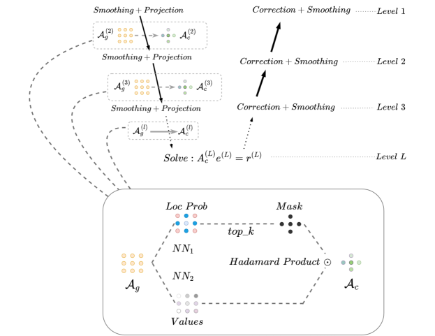
Figure 3: Illustration of the ML algorithm for computing coarse-grid operators with NNs.

Remark 3.1.

A few remarks on Algorithm 2 and Algorithm 3 follow. To begin with, the parameter $k$ of Algorithm 2 signifies the number of the nonzero entries in the sparsified stencil. This effectively gives us the ability to directly manipulate the complexity of the resulting non-Galerkin operator. Secondly, in the NN implementations, we ensure that the shapes of $\mathcal{M}^{(l)}$ and $\mathcal{V}^{(l)}$ are identical. This enables the proper application of the Hadamard product. Lastly, it is assumed that the NNs, $F_{\theta_{l}}$ and $G_{\psi_{l}}$, have undergone sufficient training. Therefore, Step 7 of Algorithm 3 involves merely the application of the trained NNs.

Algorithm 2 SparsifyStencil

0:  $\mathcal{A}_{g},F_{\theta},G_{\psi},k$

1:  Apply the NNs to compute $\mathcal{P}=F_{\theta}(\mathcal{A}_{g})$ and $\mathcal{V}=G_{\psi}(\mathcal{A}_{g})$

2:  $\mathcal{M}$ has the same shape as $\mathcal{V}$ and has a value of 1 at the entries corresponding to the $k$ largest values of $\mathcal{P}$, with 0 elsewhere.

3:  return  $\mathcal{A}_{c}=\mathcal{M}\odot\mathcal{V}$

Algorithm 3 AMG V-Cycle with sparsified coarse-grid operator

1:  Pre-smoothing: $u^{(l)}:=(I-(M^{(l)})^{-1}A^{(l)})u^{(l)}+(M^{(l)})^{-1}f^{(l)}$ for $\nu$ steps

2:  Compute the residual $r^{(l)}=f^{(l)}-A^{(l)}u^{(l)}$ and restriction $r^{(l+1)}=R^{(l)}r^{(l)}$

3:  Compute the Galerkin operator $A_{g}^{(l+1)}=R^{(l)}A^{(l)}P^{(l)}$

4:  if $l=L-1$ then

5:     Solve $A_{g}^{(l+1)}u^{(l+1)}=r^{(l+1)}$ with an arbitrary method

6:  else

7:     Apply Algorithm 2: $\mathcal{A}_{c}^{(l+1)}=\mbox{SparsifyStencil}(\mathcal{A}_{g}^{(l+1)},F_{\theta^{(l+1)}},G_{\psi^{(l+1)}},k)$

8:     Let $A^{(l+1)}=A_{c}^{(l+1)}$, $u^{(l+1)}=0$ and $f^{(l+1)}=r^{(l+1)}$. Go to Step 1 with $l:=l+1$

9:  end if

10:  Prolongate and correct: $u^{(l)}:=u^{(l)}+P^{(l)}u^{(l+1)}$

11:  Post-smoothings: $u^{(l)}:=(I-(M^{(l)})^{-\mathsf{T}}A^{(l)})u^{(l)}+(M^{(l)})^{-\mathsf{T}}f^{(l)}$ for $\nu$ steps

3.1 NN training algorithm

In this section, we delve into the specifics of the training algorithm that enables NNs to generate stencils with a higher level of sparsity compared to the Galerkin stencil, without impairing the overall convergence of the AMG method. A key component of Algorithm 3 is line 7 where $F_{\theta}$ and $G_{\psi}$ are the pre-trained NNs. The loss function, another crucial component, is pivotal to the training procedure. Based on the discussion in Section 2.3, we aim to minimize the discrepancy between $A_{g}v$ and $A_{c}v$ where $v$ is an algebraically smooth vector.

For each PDE coefficient $\beta\in\mathbb{R}^{p}$ possessing a probability distribution $p_{\beta}$ in $\mathscr{B}$, the loss function tied to $F_{\theta}$ and $G_{\psi}$ is defined as:

(17) $$\mathcal{L}_{\beta}\left(F_{\theta},G_{\psi},\mathcal{A}_{g}^{\beta},\{v^{\beta}_{j}\}_{j=1}^{s}\right)=\sum_{j=1}^{s}\lVert A_{g}^{\beta}v^{\beta}_{j}-A_{c}^{\beta}v^{\beta}_{j}\rVert_{2}^{2},$$

where $\{v^{\beta}_{j}\}$ represents the set of algebraically smooth vectors, $s$ is the number of these vectors, and $\mathcal{A}_{c}^{\beta}$ is computed by Algorithm 2. The objective is to minimize the expectation of $\mathcal{L}_{\beta}$ under the distribution of $\beta$, symbolized as $\mathbb{E}_{\beta\sim p_{\beta}}\left[\mathcal{L}_{\beta}\right]$, throughout the training. It is worth mentioning that instead of explicitly forming the matrices $A_{g}^{\beta}$ and $A_{c}^{\beta}$, we adopt a stencil-based approach where the matrix-vector multiplications are performed as the convolutions of the stencils $\mathcal{A}_{g}^{\beta}$ and $\mathcal{A}_{c}^{\beta}$ with vectors that are padded with zero layers. The stencil-based approach and the convolution formulation greatly enhance memory efficiency during training.

3.2 Details of Training and Testing

In this section, we provide details of the training and testing algorithms.

Architecture of the multi-head attention

We use multi-head attention [29] to compute both location probability in Step 1 with $F_{\theta^{(l)}}$ and numerical values in Step 2 with $G_{\theta^{(l)}}$ as discussed in Section 3. We adopt the standard architecture that comprises a set of $n_{h}$ independent attention heads, each of which extracts different features from each stencil entry of $\mathcal{A}_{g}^{(l)}$. In essence, each head generates a different learned weighted sum of the input values, where the weights are determined by the attention mechanism and reflect the importance of each value. The weights are calculated using a softmax function applied to the scaled dot-product of the input vectors. The output from each head is then concatenated and linearly transformed to produce the final output.

The multi-head attention mechanism in our study is formally defined as follows: Let $v_{g}^{(l)}$ denote the input vectors. For each attention head $h_{i},i=1,\ldots,n_{h}$, we first transform the inputs using parameterized linear transformations, $W^{Q}_{i}$, $W^{K}_{i}$, and $W^{V}_{i}$ to produce the vectors of query $Q_{i}$, key $K_{i}$, and value $V_{i}$ as follows:

(18) $$Q_{i}=v_{g}^{(l)}W^{Q}_{i},\quad K_{i}=v_{g}^{(l)}W^{K}_{i},\quad V_{i}=v_{g}^{(l)}W^{V}_{i}.$$

The attention scores for each input vector in head $h_{i}$ are then computed using the scaled dot-product of the query and key vectors, followed by a softmax function:

(19) $$\text{Attention}_{i}=\text{softmax}\left(\frac{Q_{i}K_{i}^{T}}{\sqrt{d_{k}}}\right)V_{i}\ ,$$

where $d_{k}$ is the dimension of the key vectors. This process captures the dependencies among the input vectors based on their similarities. The output of each attention head $h_{i}$ is then concatenated, and a linear transformation is applied using a parameterized weight matrix $W^{O}$ with softmax activation, which ensures positive outputs:

(20) $$\text{MultiHead}(v_{g}^{(l)})=\text{Concat}(\text{Attention}_{1},\ldots,\text{Attention}_{n_{h}})W^{O}.$$

This architecture empowers the model to learn complex PDE stencil patterns effectively. The design is flexible, and the number of heads can be adjusted as per the complexity of the task.

Intuition of selection of multi-head attention

We first briefly explain why multi-head attention is beneficial for PDE stencil learning than other types of NNs. This work is about teaching the NNs to generate stencils, which are essentially small patterns or templates used in the discretization of PDEs. These stencils represent the relationship between a grid point and its neighbors. In the context of PDE stencil learning, multi-head attention can be highly beneficial for several reasons:

1. Feature diversification: The multi-head attention allows the model to focus on various features independently, and thus, can capture a wider variety of patterns in the data. For PDE stencil learning, this means that the model can understand the relationships between different grid points more comprehensively.

2. Context awareness: Attention mechanisms inherently have the capacity to consider the context, i.e., the relationships between different parts of the input data. In PDE stencil learning, this translates to understanding the interactions between a grid point and its surrounding neighboring points.

3. Flexibility: Multi-head attention adds flexibility to the model. Each head can learn to pay attention to different features, making the model more adaptable. In the context of PDEs, this means that one head can learn to focus on local features (such as the values of nearby points), while another might focus more on global or structural aspects.

We note here that these explanations owe to the empirical observation that such an architecture works better than vanilla deep NNs on our task.

Details of training and testing

The PDE coefficient $\beta_{i}$ is sampled from distribution $\mathscr{B}$ according to the probability density function $p_{\beta}$ to get the set of $N_{t}$ parameters, $\{\beta_{i}\}$, $i=1,\ldots,{N_{t}}$. Then, we construct the corresponding set of fine-grid stencils $\{\mathcal{A}^{\beta_{i}}\}$. For all the tests in this paper, we use full coarsening, full-weighting restriction, and the corresponding bi-linear interpolation for all the levels of AMG. At each level $l>1$, the ML model is built with the Galerkin stencils $\{(\mathcal{A}_{g}^{\beta_{i}})^{(l)}\}$ and a set of smooth test vectors $\{(v_{j}^{\beta_{i}})^{(l)}\}$, $j=1,\ldots,{s_{l}}$, associated with each of the stencil, using the loss function

(21) $$\mathcal{L}=\frac{1}{N_{t}}\sum_{i=1}^{N_{t}}\mathcal{L}_{\beta_{i}}\left(F_{\theta^{(l)}},G_{\psi^{(l)}},(\mathcal{A}_{g}^{\beta_{i}})^{(l)},\{(v^{\beta_{i}}_{j})^{(l)}\}\right)$$

that is used to approximate $\mathbb{E}_{\beta\sim p_{\beta}}\left[\mathcal{L}_{\beta}\right]$. The complete training procedure is summarized in Algorithm 4. It is important to note that the NN trainings are independent of each other on different levels. Therefore, the training of the NNs for each level can be carried out simultaneously once the training data is prepared, taking advantage of parallel computing resources. The testing set is constructed with parameters that differ from those in the training set. This means that we test the model on a set of PDE parameters $\{\beta_{j}\}$, $j=1,\ldots,{N_{v}}$, that have not been encountered by the models during training. The purpose of the testing set is to assess the generalization capability of new problem instances.

Algorithm 4 Training NNs for computing coarse-grid operator at level $l$

0:  Interpolation operator $P^{(l)}$, Galerkin coarse-grid stencils $\{(\mathcal{A}_{g}^{\beta_{i}})^{(l)}\}$, the number of test vectors $s_{l}$ and the target stencil complexity $k$

0:  NNs $F_{\theta^{(l)}}$ and $G_{\psi^{(l)}}$

1:  Generate test vectors $(v^{\beta_{i}}_{j})^{(l)}$, $j=1,\ldots,s_{l}$, for each $(\mathcal{A}_{g}^{\beta_{i}})^{(l)}$ as follows

• Compute $T^{(l)}=(P^{(l)})^{\mathsf{T}}P^{(l)}$

• Compute the eigenvalues and vectors of

  $$(A_{g}^{\beta_{i}})^{(l)}u=\lambda_{i}^{(l)}T^{(l)}u$$

• The test vectors are the eigenvectors associated with the $s_{l}$ smallest eigenvalues

2:  Initialize $G_{\theta^{(l)}}$ and $G_{\psi^{(l)}}$

3:  repeat

4:     Apply Algorithm 2: $(\mathcal{A}_{c}^{\beta_{i}})^{(l)}=\mbox{SparsifyStencil}\left((\mathcal{A}_{g}^{\beta_{i}})^{(l)},F_{\theta^{(l)}},G_{\psi^{(l)}},k\right)$

5:     Compute the gradient of the loss Eq. 21

6:     Update the weights $\theta^{(l)}$ and $\psi^{(l)}$

7:  until the prescribed number of training epochs is reached

4 Numerical Results

We report the numerical results of the proposed ML-based non-Galerkin coarse-grid method in this section. All the ML models in the work were written with PyTorch 1.9.0 [24]. We use PyAMG 4.2.3 [2] to build the AMG hierarchy. All the experiments were performed on a workstation with Intel Core i7-6700 CPUs.

4.1 Evaluation Metrics

In this section, we evaluate the performance of the proposed ML-based approach by comparing the average number of iterations required by the AMG method using different coarse-grid operators to converge. Additionally, we verify the spectral equivalence of the Galerkin and sparsified non-Galerkin stencils by computing the spectra of the corresponding matrices on meshes of various sizes.

4.2 Spectrally equivalent stencils

We first examine the proposed ML-based method on the 9-point stencil problem Eq. 8 that allows direct evaluation of the learned non-Galerkin operator by the comparison with the theoretical result Eq. 9, which is a spectrally equivalent 5-point stencil. We use the 9-point stencil $\mathcal{A}$ of the form Eq. 8 with $a=2.720$, $b=1.417$ and $c=0.000114$, i.e.,

(25) $$\mathcal{A} =\left[\begin{array}[]{ccc}0.000114&2.720&0.000114\\ 1.417&-8.275&1.417\\ 0.000114&2.720&0.000114\\ \end{array}\right]$$

as the fine-level $A$-operator, and the 2-D full-weighting stencil,

(26) $$\mathcal{R}=\dfrac{1}{4}\begin{bmatrix}1&2&1\\ 2&4&2\\ 1&2&1\end{bmatrix},$$

for the restriction operator. Thus, the stencil of the Galerkin operator is

(27) $$\mathcal{A}_{g}=\left[\begin{array}[]{ccc}0.129&0.096&0.129\\ 0.422&-1.551&0.422\\ 0.129&0.096&0.129\\ \end{array}\right],$$

which has the same form as $\mathcal{A}$. From Eq. 9, a 5-point stencil that is spectrally equivalent to Eq. 27 is given by

(28) $$\mathcal{A}_{c}=\begin{bmatrix}0&0.354&0\\ 0.680&-2.069&0.680\\ 0&0.354&0\end{bmatrix}.$$

Using Algorithm 4 with the prescribed stencil complexity $k=5$ on the $31\times 31$ grid, the pre-trained NNs produced the following 5-point stencil

(29) $$\mathcal{A}_{nn}=\begin{bmatrix}0&0.348&0\\ 0.666&-2.024&0.663\\ 0&0.347&0\end{bmatrix},$$

denoted by $\mathcal{A}_{nn}$, which is close to the theoretical result Eq. 28. To assess the convergence behavior of the AMG method, we solve a linear system using the coefficient matrix defined by (25). We conduct these tests on larger-sized grids and use the two-grid AMG methods employing $\mathcal{A}_{g}$, $\mathcal{A}_{c}$, and $\mathcal{A}_{nn}$ as the coarse-level operators, respectively. The right-hand-side vector is generated randomly. The stopping criterion with respect to the relative residual norm is set to be $10^{-6}$. The results are shown in Table 1, from which we can observe that all three methods require the same number of iterations.

Table 1: The number of iterations required by the two-level AMG methods for solving a linear system corresponding to the coefficient matrix stencil (25) to $10^{-6}$ accuracy in terms of the relative residual. The AMG methods utilize $\mathcal{A}_{g}$, $\mathcal{A}_{c}$, and $\mathcal{A}_{nn}$ as the coarse-level operator respectively. The tests are carried out on grid sizes up to $511\times 511$.

	grid size
	63	95	127	191	255	383	511
$\mathcal{A}_{g}$	11	10	10	10	10	10	10
$\mathcal{A}_{c}$	11	10	10	10	10	10	10
$\mathcal{A}_{nn}$	11	10	10	10	10	10	10

4.3 2-D rotated Laplacian problem

In this section, we consider the 2-D anisotropic rotated Laplacian problem

(30) $$-\nabla\cdot(T_{\theta,\xi}\nabla u(x,y))=f(x,y),$$

where the $2\times 2$ vector field $T_{\theta,\xi}$ parameterized by $\theta$ and $\xi$ is defined as

$$T_{\theta,\xi}=\begin{bmatrix}\cos^{2}{\theta}+\xi\sin^{2}{\theta}&\cos{\theta}\sin{\theta}(1-\xi)\\ \cos{\theta}\sin{\theta}(1-\xi)&\sin^{2}{\theta}+\xi\cos^{2}{\theta}\end{bmatrix}$$

with $\theta$ being the angle of the anisotropy and $\xi$ being the conductivity.

We show that the proposed approach is not limited to a particular set of parameters but remains effective across a range of values for both $\xi$ and $\theta$. In the first set of experiments, we fix the value $\xi$ while allowing $\theta$ to follow a uniform distribution within a specified interval. We conduct 12 experiments where each $\xi\in\{100,200,300,400\}$ is paired up with $\theta$ sampled from intervals $\{({\pi}/{4},{\pi}/{3}),({\pi}/{3},{5\pi}/{12}),({\pi}/{2},{7\pi}/{12})\}$. The AMG methods for solving these problems use full-coarsening, full-weighting restriction, and the Gauss-Seidel method for both pre-smoothing and post-smoothing. AMG V-cycles are executed until the residual norm is reduced by $6$ orders of magnitude. The number of the nonzero elements is $9$ in the Galerkin coarse-grid stencil across the AMG levels, whereas we choose to reduce the number to $5$ for the non-Galerkin operator.

During the training phase of each experiment, the model is provided with 5 distinct instances that share the same $\xi$ but have different $\theta$ values evenly distributed within the chosen interval. For example, for $\xi=100$ and $\theta\in({\pi}/{4},{\pi}/{3})$, the parameters for the $5$ instances of $(\xi,\theta)$ are selected as follows:

(31) $$\left\{(100,{\pi}/{4}),(100,{3.25\pi}/{12}),(100,{3.5\pi}/{12}),(100,{3.75\pi}/{12}),(100,{\pi}/{3})\right\}.$$

The size of the fine-level matrix in the training instances is set to be $31\times 31$. In the testing phase, $10$ distinct $\theta$ values are randomly selected from the chosen interval. The AMG parameters are consistent with those used in the training phase. In the testing, it should be noted that the fine-level problem size is $511\times 511$, which is approximately 256 times larger than that in the training instances. This larger problem size in the testing allows for a more rigorous evaluation of the performance of AMG and the ability to handle larger-scale problems. We record the number of iterations required by the 3-level AMG method to converge with the Galerkin and non-Galerkin operators, shown in Table 2. These results indicate that the convergence behavior of the AMG method remains largely unchanged when the alternative sparser non-Galerkin coarse-grid operators are used as replacements.

Table 2: The average number of iterations required by the 3-level AMG to converge with the Galerkin and non-Galerkin coarse-grid operators for solving (30) with different PDE parameter $\xi$ and $\theta$. The mesh size is $511\times 511$. The parameters are selected so that $\xi\in\{100,200,300,400\}$ is fixed and $\theta$ is randomly sampled from a uniform distribution in each interval. The iteration number is averaged over 10 different sampled $\theta$ values.

	$\xi$	$\theta$
		(${\pi}/{6}$, ${\pi}/{4}$)	(${\pi}/{4}$,${\pi}/{3}$)	(${\pi}/{2}$, ${7\pi}/{12}$)
$\mathcal{A}_{g}$	100	92.1	102.8	126.9
${\mathcal{A}_{nn}}$		89.0	93.0	135.2
$\mathcal{A}_{g}$	200	191.7	196.6	203.1
${\mathcal{A}_{nn}}$		174.2	177.8	204.9
$\mathcal{A}_{g}$	300	248.0	269.7	342.3
${\mathcal{A}_{nn}}$		246.5	231.4	356.2
$\mathcal{A}_{g}$	400	337.1	351.1	438.2
${\mathcal{A}_{nn}}$		326.3	327.7	441.5

In the second set of experiments, we keep the parameter $\theta$ fixed and vary $\xi$ following a uniform distribution within the selected intervals. A total of 12 experiments were conducted where each $\theta\in\{{\pi}/{6},{\pi}/{4},{\pi}/{3},{5\pi}/{12}\}$ is paired with $\xi$ sampled from the intervals $\{(5,10),(80,100),(100,200)\}$. The AMG configurations used in these experiments remain the same as in the previous set. The training and testing processes are also similar. For each experiment, we train the model using 5 different instances evenly distributed within the selected intervals and then test it with 10 randomly sampled $\xi$ values from the same interval. The size of the fine-level linear system in the training instances is set to be $31\times 31$, while in each testing instance, it has a much larger size that is $511\times 511$. The averaged numbers of iterations from all the experiments are presented in Table 3.

Table 3: The average number of iterations required by the 3-level AMG to converge with the Galerkin and non-Galerkin coarse-grid operators for solving (30) with different PDE parameter $\xi$ and $\theta$. The mesh size is $511\times 511$. The parameters are selected such that $\theta\in\{{\pi}/{6},{\pi}/{4},{\pi}/{3},{5\pi}/{12}\}$ is fixed and $\xi$ is randomly sampled from a uniform distribution in each interval. The iteration number is averaged over 10 different sampled $\xi$ values.

	$\theta$	$\xi$
		(100, 200)	(80, 100)	(5, 10)
$\mathcal{A}_{g}$	$\pi/6$	90.4	72.1	13.5
${\mathcal{A}_{nn}}$		100.2	84.4	13.8
$\mathcal{A}_{g}$	$\pi/4$	172.5	105.2	14.1
${\mathcal{A}_{nn}}$		123.1	79.0	15.9
$\mathcal{A}_{g}$	$\pi/3$	99.4	80.9	14.3
${\mathcal{A}_{nn}}$		79.1	88.8	15.4
$\mathcal{A}_{g}$	$5\pi/12$	92.5	76.4	16.5
${\mathcal{A}_{nn}}$		107.4	88.2	16.6

In the subsequent experiment, we specifically consider the Laplacian problem with parameters $\theta={\pi}/{6}$ and $\xi=0.1$ as an example to demonstrate the measurement of spectral equivalence as defined in Eq. 2. We examine the eigenvalues of $A_{nn}^{-1}A_{g}$ on meshes of varying sizes, as depicted in Fig. 4. We observe that all the eigenvalues are approximately equal to 1, and the distribution of eigenvalues remains consistent regardless of the mesh size. This observation suggests the presence of spectral equivalence between the two coarse-grid operators across meshes of different sizes.

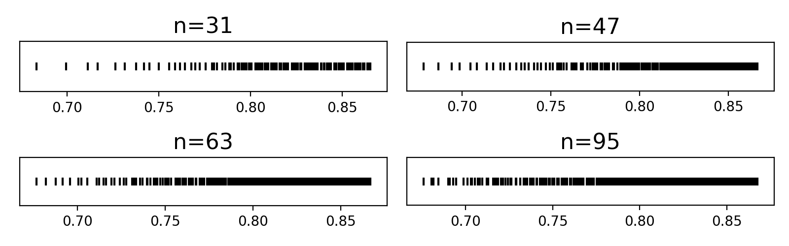
Figure 4: The eigenvalues of $A_{nn}^{-1}A_{g}$ on meshes of different sizes ($n\times n$) for solving the rotated Laplacian problem with $\theta={\pi}/{6}$ and $\xi=0.1$.

The target stencil complexity $k$ in Algorithm 2 is a parameter left to be chosen by the users. It is an adjustable parameter that allows users to control the sparsity level in the trained NN-model and of the resulting coarse-grid operator. The appropriate value of $k$ typically depends on the problem domain and the desired balance between accuracy and computational efficiency. It may be necessary to perform experiments to determine the optimal value of $k$ for a particular application. In the final experiment, we perform this study for the rotated Laplacian problem with $\xi=10$ and $\theta={\pi}/{4}$. Note that the Galerkin operator has a 9-point stencil, so we vary the stencil complexity from $4$ to $6$ in the non-Galerkin operator and record the convergence behavior of the corresponding AMG method. The results, as depicted in Fig. 5, show the findings regarding the convergence behavior of the AMG method with different values of $k$ in the sparsified stencil $\mathcal{A}_{nn}$. Notably, when $k=4$, the AMG method fails to converge. However, for $k=5$ and $k=6$, the convergence behavior closely resembles that of the 9-point Galerkin operator. This observation suggests that a minimum stencil complexity of $k=5$ appears to be required for $\mathcal{A}_{nn}$ to achieve convergence, which coincides with the operator complexity of the fine-grid operator.

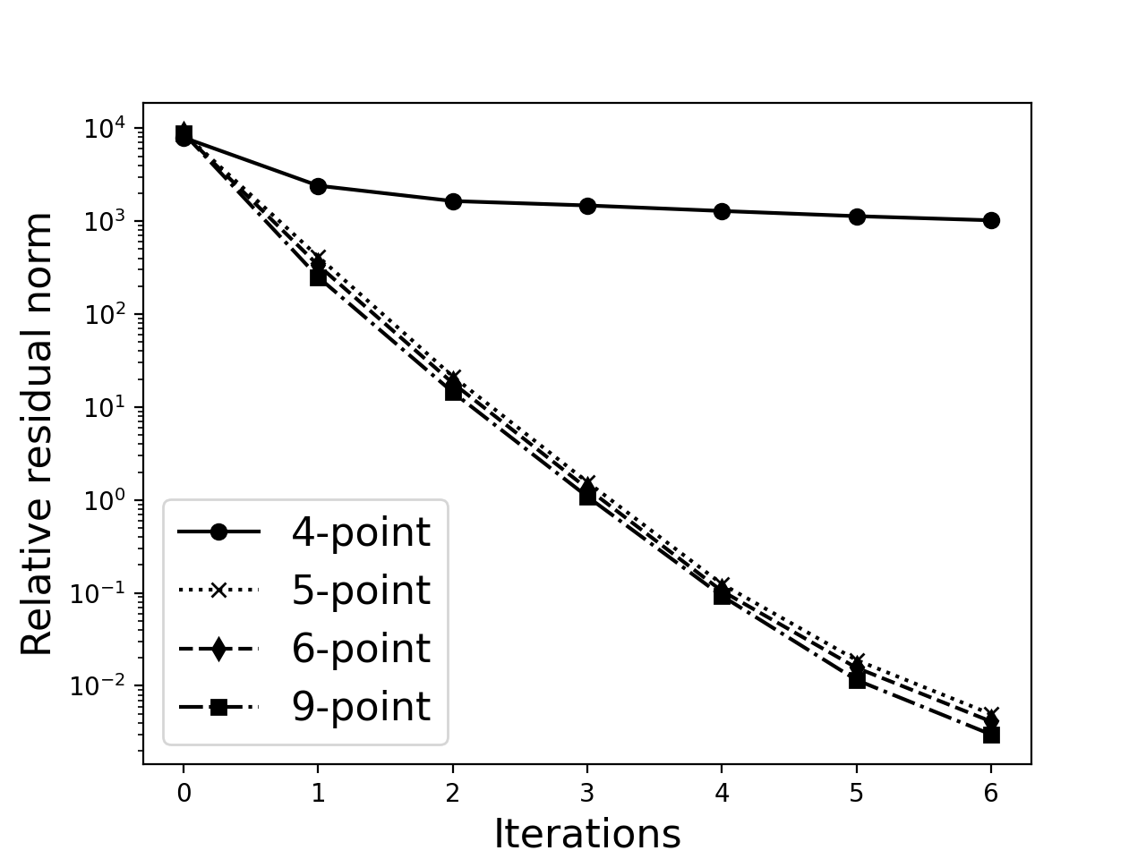
Figure 5: The convergence in terms of the residual norm of the two-grid AMG methods using the coarse-grid operator from the NN model of stencil complexity $k=4,5,6$ and the Galerkin operator for solving the rotated Laplacian problem with $\xi=10$ and $\theta={\pi}/{4}$.

4.4 2-D linear elasticity problem

In this section, we consider the 2-D time-independent linear elasticity problem in an isotropic homogeneous medium:

(32) $$\mu\nabla^{2}u+(\mu+\lambda)(\frac{\partial^{2}u}{\partial x^{2}}+\frac{\partial^{2}v}{\partial x\partial y})+f_{x} =0,$$

(33) $$\mu\nabla^{2}v+(\mu+\lambda)(\frac{\partial^{2}v}{\partial x^{2}}+\frac{\partial^{2}u}{\partial x\partial y})+f_{y} =0,$$

where $u$ and $v$ are the solution in the direction of $x$- and $y$-axis respectively, $f_{x}$ and $f_{y}$ are forcing terms, and $\mu$ and $\lambda$ are Lame coefficients that are determined by Young’s modulus $E$ and Poisson’s ratio $\nu$ as

(34) $$\mu=\frac{E}{2(1+\nu)}\ ,\quad\lambda=\frac{E\nu}{(1+\nu)(1-2\nu)}\ .$$

In our tests, we set $E=10^{-5}$ and vary the value of $\nu$. For the discretization, we adopt the optimal 2-D 9-point stencil in terms of local truncation errors [20] on rectangular Cartesian grid with the mesh step sizes $h$ and $b_{y}h$, respectively, along the $x$- and $y$-axes ($b_{y}$ is the aspect ratio of the mesh),

(35) $$\mathcal{A}_{uu} =\begin{bmatrix}a_{uu}^{nw}&a_{uu}^{n}&a_{uu}^{ne}\\ a_{uu}^{w}&1&a_{uu}^{e}\\ a_{uu}^{sw}&a_{uu}^{s}&a_{uu}^{se}\\ \end{bmatrix},\quad\mathcal{A}_{uv}=\begin{bmatrix}a_{uv}^{nw}&0&a_{uv}^{ne}\\ 0&0&0\\ a_{uv}^{sw}&0&a_{uv}^{se}\\ \end{bmatrix},\;$$

where the coefficients are given by

(36) $$a_{uu}^{n} =a_{uu}^{s}=\frac{(b_{y}^{2}-1)\lambda+2(b_{y}^{2}-2)\mu}{2(2\lambda b_{y}^{2}+\lambda+4(b_{y}^{2}+1)\mu)}\ ,$$

(37) $$a_{uu}^{w} =a_{uu}^{e}=-\frac{2\lambda b_{y}^{2}+4\mu b_{y}^{2}+\lambda+\mu}{2(2\lambda b_{y}^{2}+\lambda+4(b_{y}^{2}+1)\mu)}\ ,$$

(38) $$a_{uu}^{nw} =a_{uu}^{ne}=a_{uu}^{sw}=a_{uu}^{se}=\frac{-\lambda b_{y}^{2}-2\mu b_{y}^{2}+\lambda+\mu}{4(2\lambda b_{y}^{2}+\lambda+4(b_{y}^{2}+1)\mu)}\ ,$$

(39) $$a_{uv}^{nw} =a_{uv}^{se}=-a_{uv}^{ne}=-a_{uv}^{sw}=\frac{3b_{y}(\lambda+\mu)}{8(2\lambda b_{y}^{2}+\lambda+4(b_{y}^{2}+1)\mu)}\ .$$

These stencils define the $2\times 2$ block linear system

(40) $$\begin{bmatrix}A_{uu}&A_{uv}\\ A_{vu}&A_{vv}\end{bmatrix}\begin{bmatrix}u\\ v\end{bmatrix}=\begin{bmatrix}f_{x}\\ f_{y}\end{bmatrix},$$

where ${A}_{uu}={A}_{vv}$ and ${A}_{vu}={A}_{uv}^{\mathsf{T}}$. A node-based AMG approach is used to solve Eq. 40, where the same red-black coarsening is used in $u\mathchar 45\relax u$ and $v\mathchar 45\relax v$ blocks and the interpolation and restriction operators have the same block form

(41) $$R=\begin{bmatrix}R_{uu}&R_{uv}\\ R_{vu}&R_{vv}\end{bmatrix},\quad P=\begin{bmatrix}P_{uu}&P_{uv}\\ P_{vu}&P_{vv}\end{bmatrix},$$

which interpolate and restrict within and across the two types of variables $u$ and $v$. The stencils of the operators in Eq. 41 are given by, respectively,

(48) $$\mathcal{R}_{uu} =\mathcal{R}_{vv}=\frac{1}{8}\left[\begin{array}[]{ccc}&1&\\ 1&4&1\\ &1&\\ \end{array}\right],\quad\mathcal{P}_{uu}=\mathcal{P}_{vv}=\frac{1}{4}\left]\begin{array}[]{ccc}&1&\\ 1&4&1\\ &1&\\ \end{array}\right[\ ,$$

(55) $$\mathcal{R}_{uv} =\frac{1}{8}\left[\begin{array}[]{ccc}&1&\\ -1&0&-1\\ &1&\\ \end{array}\right],\quad\mathcal{P}_{uv}=\frac{1}{4}\left]\begin{array}[]{ccc}&1&\\ -1&0&-1\\ &1&\\ \end{array}\right[\ ,$$

(62) $$\mathcal{R}_{vu} =\frac{1}{8}\left[\begin{array}[]{ccc}&-1&\\ 1&0&1\\ &-1&\\ \end{array}\right],\quad\mathcal{P}_{vu}=\frac{1}{4}\left]\begin{array}[]{ccc}&-1&\\ 1&0&1\\ &-1&\\ \end{array}\right[\ .$$

As stated in [7], to interpolate exactly the smoothest function that is locally constant, it requires the interpolation weights for $u\mathchar 45\relax u$ and $v\mathchar 45\relax v$ to sum to 1 and for the $u\mathchar 45\relax v$ and $v\mathchar 45\relax u$ weights to sum to 0. The Gauss-Seidel smoother is used with the AMG V-cycle and the iterations are stopped when the relative residual norm is below $10^{-6}$.

We train the NN model on 4 different instances with $\nu\in\{0.1,0.2,0.3,0.4\}$ to reduce the complexity of the Galerkin operator by 50%. The coarse-grid Galerkin operator has the same block structure as Eq. 40 and only 2 distinct stencils due to the symmetry of the matrix. In the training, we combine these 2 stencils and pass them to the NNs as the input. It turns out that the NN model trained in this way yields better coarse-grid operators than learning the stencils of $u\mathchar 45\relax u$ and $u\mathchar 45\relax v$ separately.

The mesh size used in the training set is set to be $9\times 9$. We test the model on instances with $\nu$ randomly drawn from each interval of $\{(0.1,0.2),(0.2,0.3),(0.3,0.4)\}$. The size of the mesh used in the testing is $65\times 65$. The average numbers of iterations are presented in Table 4. Similar to the results observed in the rotated Laplacian problems, the convergence behavior of the two-grid AMG method is not negatively affected by the replacement with the non-Galerkin coarse-grid operator obtained from the NN model.

Table 4: The average number of iterations required by the 2-grid AMG to converge with the Galerkin and non-Galerkin coarse-grid operators for solving (32) with 10 different Poisson’s ratios $\nu$ randomly sampled from each interval. The mesh size is set to be $65\times 65$.

$\nu$	$(0.1,0.2)$	$(0.2,0.3)$	$(0.3,0.4)$
$\mathcal{A}_{g}$	10.1	10.2	10.6
${\mathcal{A}_{nn}}$	11.0	10.7	11.5

4.5 Comparison with existing non-Galerkin methods

In this section, we compare the performance of the proposed NN-based algorithm with the Sparsified Smooth Aggregation (SpSA) method proposed in [27] for solving the rotated Laplacian problem. The SpSA method is based on Smooth Aggregation (SA) AMG methods. In these methods, a tentative aggregation-based interpolation operator $P_{t}$ is first constructed, followed by a few steps of smoothing of $P_{t}$ that generate the final interpolation operator $P$, which is typically considerably denser than $P_{t}$. The SpSA algorithm aims to reduce the complexity of the Galerkin operator $P^{\mathsf{T}}AP$ to have the same sparsity pattern as $P_{t}^{\mathsf{T}}AP_{t}$. Given that we utilize the standard Ruge-Stüben AMG (as opposed to SA AMG) combined with the NN-based approach, conducting a direct comparison between the two approaches becomes challenging due to the different AMG hierarchies obtained. To ensure an equitable comparison, we impose a requirement that the number of nonzero entries per row in the coarse-level operator generated by SpSA should not be smaller than the operator produced by our algorithm. Consequently, any observed disparities in performance can be attributed to the specific characteristics of the selected sparsity pattern and numerical values of the coarse-grid operator, rather than the variations in the level of the sparsity. The number of iterations required by the GMRES method preconditioned by 3-level AMG methods with different coarse-grid operators for solving the rotated Laplacian problem (30) are presented in Table 5 and Table 6, with varied PDE coefficients. For the majority of cases, the AMG method with NN-based coarse-grid operators exhibits better performance compared to SpSA, as it requires fewer iterations to converge to the $10^{-6}$ stopping tolerance and achieves convergence rate that is much closer to that using the Galerkin operator. There are a few exceptions where SpSA outperforms the NN-based method, and in some cases, it performs even better than the AMG method using the Galerkin operator.

Table 5: The average number of iterations required by the GMRES method preconditioned by 3-level AMG methods with different coarse-grid operators for solving (30) with different sets of PDE parameters. The mesh size is $511\times 511$. The parameters are selected so that $\theta\in\{{\pi}/{6},{\pi}/{4},{\pi}/{3},{5\pi}/{12}\}$ is fixed and $\xi$ is randomly sampled from a uniform distribution in each interval. The iteration number is averaged over 10 different sampled $\theta$’s. $\mathcal{A}_{g}$ denotes the Galerkin coarse-grid operator, $\mathcal{A}_{nn}$ is the coarse-grid operator obtained from Algorithm 4, and SpSA refers to the coarse-grid operator from the Sparsified Smooth Aggregation (SpSA) algorithm [27].

	$\xi$	$\theta$
		(${\pi}/{6}$, ${\pi}/{4}$)	(${\pi}/{4}$,${\pi}/{3}$)	(${\pi}/{2}$, ${7\pi}/{12}$)
$\mathcal{A}_{g}$	100	11.3	11.1	11.5
${\mathcal{A}_{nn}}$		16.5	16.9	19.9
SpSA		40.4	36.9	11.5
$\mathcal{A}_{g}$	200	15.9	15.3	14.5
${\mathcal{A}_{nn}}$		20.5	19.6	29.8
SpSA		50.4	46.7	9.1
$\mathcal{A}_{g}$	300	18.1	21.5	17.9
${\mathcal{A}_{nn}}$		25.4	33.1	25.6
SpSA		53.0	52.1	12.3
$\mathcal{A}_{g}$	400	21.1	20.2	19.9
${\mathcal{A}_{nn}}$		27.2	30.9	26.2
SpSA		59.7	56.3	12.9

Table 6: The average number of iterations required by the GMRES method preconditioned by 3-level AMG methods with different coarse-grid operators for solving (30) with different sets of PDE parameters. The mesh size is $511\times 511$. The parameters are selected so that $\theta\in\{\pi/6,\pi/4,\pi/3,5\pi/12\}$ is fixed and $\xi$ is randomly sampled from a uniform distribution in each interval. The iteration number is averaged over 10 different sampled $\xi$’s. $\mathcal{A}_{g}$ denotes the Galerkin coarse-grid operator, $\mathcal{A}_{nn}$ is the coarse-grid operator obtained from Algorithm 4, and SpSA refers to the coarse-grid operator from the Sparsified Smooth Aggregation (SpSA) algorithm [27].

	$\theta$	$\xi$
		($100,200$)	($80,100$)	($5,10$)
$\mathcal{A}_{g}$	$\pi/6$	11.6	10.4	4.4
${\mathcal{A}_{nn}}$		19.9	16.4	7.1
SpSA		30.3	27.0	12.7
$\mathcal{A}_{g}$	$\pi/4$	14.2	11.3	4.6
${\mathcal{A}_{nn}}$		18.2	15.5	10.0
SpSA		41.4	34.7	13.5
$\mathcal{A}_{g}$	$\pi/3$	11.2	10.2	4.7
${\mathcal{A}_{nn}}$		18.8	16.4	7.1
SpSA		31.7	28.9	13.4
$\mathcal{A}_{g}$	$5\pi/12$	11.2	10.1	4.8
${\mathcal{A}_{nn}}$		28.8	19.1	9.1
SpSA		16.5	15.1	9.1

5 Conclusion

In this work, we propose an ML-based approach for computing non-Galerkin coarse-grid operators to address the issue of increasing operator complexity in AMG methods by sparsifying the Galerkin operator in different AMG levels. The algorithm consists of two main steps: choosing the sparsity pattern of the stencil and computing the numerical values. We employ NNs in both steps and combine their results to construct a non-Galerkin coarse-grid operator with the desired lower complexity. The NN training algorithm is guided by the AMG convergence theory, ensuring the spectral equivalence of coarse-grid operators with respect to the Galkerkin operator. We showed that spectrally equivalent sparser stencils can be learned by advanced ML techniques that exploit multi-head attention.

The NN model is trained on parametric PDE problems that cover a wide range of parameters. The training dataset consists of small-size problems, while the testing problems are significantly larger. Empirical studies conducted on rotated Laplacian and linear elasticity problems provide evidence that the proposed ML method can construct non-Galerkin operators with reduced complexity while maintaining the overall convergence behavior of AMG. A key feature of our method is its ability to generalize to problems of larger sizes and with different PDE parameters that were not encountered in the training. This means that the algorithm can effectively handle a wide range of problem settings, expanding its practical applicability. By generalizing to new problem instances, the algorithm amortizes the training cost and reduces the need for retraining for every specific problem scenario.

In the future, we plan to extend this work to sparsify unstructured coarse grid operators by exploiting the Graph Convolution Networks (GCNs). We also plan to explore the Equivariant Neural Networks [9] to enforce the symmetry in the sparsified coarse-grid operators if the fine level operator is symmetric. Finally, we plan to investigate the real world applications including saddle point system[16], efficient tensor algebra [14, 18, 12], modern generative models [8, 17, 15], multi-time series analysis techniques [13, 25] to solve time-dependent PDEs.

References

- [1] O. Axelsson, On multigrid methods of the two-level type, in Multigrid methods, Springer, 1982, pp. 352–367.
- [2] N. Bell, L. N. Olson, and J. Schroder, Pyamg: algebraic multigrid solvers in python, Journal of Open Source Software, 7 (2022), p. 4142.
- [3] A. Bienz, R. D. Falgout, W. Gropp, L. N. Olson, and J. B. Schroder, Reducing parallel communication in algebraic multigrid through sparsification, SIAM Journal on Scientific Computing, 38 (2016), pp. S332–S357.
- [4] A. Bienz, W. D. Gropp, and L. N. Olson, Reducing communication in algebraic multigrid with multi-step node aware communication, The International Journal of High Performance Computing Applications, 34 (2020), pp. 547–561.
- [5] M. Bolten and A. Frommer, Structured grid AMG with stencil-collapsing for d-level circulant matrices. Bergische Universität Wuppertal, Wuppertal, Germany. Preprint BUW-SC 07/4, 2007.
- [6] A. Brandt, J. Brannick, K. Kahl, and I. Livshits, Bootstrap AMG, SIAM Journal on Scientific Computing, 33 (2011), pp. 612–632.
- [7] M. Brezina, A. J. Cleary, R. D. Falgout, V. E. Henson, J. E. Jones, T. A. Manteuffel, S. F. McCormick, and J. W. Ruge, Algebraic multigrid based on element interpolation (AMGe), SIAM Journal on Scientific Computing, 22 (2001), pp. 1570–1592.
- [8] D. Cai, Y. Ji, H. He, Q. Ye, and Y. Xi, Autm flow: atomic unrestricted time machine for monotonic normalizing flows, in Proceedings of the Thirty-Eighth Conference on Uncertainty in Artificial Intelligence, J. Cussens and K. Zhang, eds., vol. 180 of Proceedings of Machine Learning Research, PMLR, 01–05 Aug 2022, pp. 266–274.
- [9] T. Cohen and M. Welling, Group equivariant convolutional networks, in Proceedings of The 33rd International Conference on Machine Learning, M. F. Balcan and K. Q. Weinberger, eds., vol. 48 of Proceedings of Machine Learning Research, PMLR, 2016, pp. 2990–2999.
- [10] R. D. Falgout and J. B. Schroder, Non-galerkin coarse grids for algebraic multigrid, SIAM Journal on Scientific Computing, 36 (2014), pp. C309–C334.
- [11] D. Greenfeld, M. Galun, R. Basri, I. Yavneh, and R. Kimmel, Learning to optimize multigrid PDE solvers, in International Conference on Machine Learning, PMLR, 2019, pp. 2415–2423.
- [12] H. He, J. Henderson, and J. C. Ho, Distributed tensor decomposition for large scale health analytics, in The World Wide Web Conference, WWW ’19, New York, NY, USA, 2019, Association for Computing Machinery, p. 659–669.
- [13] H. He, O. Queen, T. Koker, C. Cuevas, T. Tsiligkaridis, and M. Zitnik, Domain adaptation for time series under feature and label shifts, in International Conference on Machine Learning, 2023.
- [14] H. He, Y. Xi, and J. C. Ho, Fast and accurate tensor decomposition without a high performance computing machine, in 2020 IEEE International Conference on Big Data (Big Data), 2020, pp. 163–170.
- [15] H. He, S. Zhao, Y. Xi, and J. Ho, AGE: Enhancing the convergence on GANs using alternating extra-gradient with gradient extrapolation, in NeurIPS 2021 Workshop on Deep Generative Models and Downstream Applications, 2021.
- [16] H. He, S. Zhao, Y. Xi, J. Ho, and Y. Saad, GDA-AM: ON THE EFFECTIVENESS OF SOLVING MIN-IMAX OPTIMIZATION VIA ANDERSON MIXING, in International Conference on Learning Representations, 2022.
- [17] H. He, S. Zhao, Y. Xi, and J. C. Ho, Meddiff: Generating electronic health records using accelerated denoising diffusion model, 2023, https://arxiv.org/abs/2302.04355.
- [18] J. Henderson, H. He, B. A. Malin, J. C. Denny, A. N. Kho, J. Ghosh, and J. Ho, Phenotyping through semi-supervised tensor factorization (psst), AMIA … Annual Symposium proceedings. AMIA Symposium, 2018 (2018), pp. 564–573.
- [19] R. Huang, R. Li, and Y. Xi, Learning optimal multigrid smoothers via neural networks, SIAM Journal on Scientific Computing, 45 (2023), pp. S199–S225.
- [20] A. Idesman and B. Dey, Compact high-order stencils with optimal accuracy for numerical solutions of 2-d time-independent elasticity equations, Computer Methods in Applied Mechanics and Engineering, 360 (2020), p. 112699.
- [21] A. Katrutsa, T. Daulbaev, and I. Oseledets, Black-box learning of multigrid parameters, Journal of Computational and Applied Mathematics, 368 (2020), p. 112524.
- [22] D. Kuznichov, Learning relaxation for multigrid, arXiv preprint arXiv:2207.11255, (2022).
- [23] I. Luz, M. Galun, H. Maron, R. Basri, and I. Yavneh, Learning algebraic multigrid using graph neural networks, in International Conference on Machine Learning, PMLR, 2020, pp. 6489–6499.
- [24] A. Paszke, S. Gross, F. Massa, A. Lerer, J. Bradbury, G. Chanan, T. Killeen, Z. Lin, N. Gimelshein, L. Antiga, et al., Pytorch: An imperative style, high-performance deep learning library, Advances in neural information processing systems, 32 (2019).
- [25] O. Queen, T. Hartvigsen, T. Koker, H. He, T. Tsiligkaridis, and M. Zitnik, Encoding time-series explanations through self-supervised model behavior consistency, 2023, https://arxiv.org/abs/2306.02109.
- [26] A. Taghibakhshi, S. MacLachlan, L. Olson, and M. West, Optimization-based algebraic multigrid coarsening using reinforcement learning, Advances in Neural Information Processing Systems, 34 (2021), pp. 12129–12140.
- [27] E. Treister and I. Yavneh, Non-galerkin multigrid based on sparsified smoothed aggregation, SIAM Journal on Scientific Computing, 37 (2015), pp. A30–A54.
- [28] E. TREISTER, R. Zemach, and I. YAVNEH, Algebraic collocation coarse approximation (acca) multigrid, in 12th Copper Mountain Conference on Iterative Methods, 2012.
- [29] A. Vaswani, N. Shazeer, N. Parmar, J. Uszkoreit, L. Jones, A. N. Gomez, L. u. Kaiser, and I. Polosukhin, Attention is all you need, in Advances in Neural Information Processing Systems, I. Guyon, U. V. Luxburg, S. Bengio, H. Wallach, R. Fergus, S. Vishwanathan, and R. Garnett, eds., vol. 30, Curran Associates, Inc., 2017.
- [30] R. Wienands and I. Yavneh, Collocation coarse approximation in multigrid, SIAM Journal on Scientific Computing, 31 (2009), pp. 3643–3660.