Evaluation of Deep Reinforcement Learning Algorithms for Portfolio Optimisation

Abstract

We evaluate benchmark deep reinforcement learning (DRL) algorithms on the task of portfolio optimisation under a simulator. The simulator is based on correlated geometric Brownian motion (GBM) with the Bertsimas-Lo (BL) market impact model. Using the Kelly criterion (log utility) as the objective, we can analytically derive the optimal policy without market impact and use it as an upper bound to measure performance when including market impact. We found that the off-policy algorithms DDPG, TD3 and SAC were unable to learn the right Q function due to the noisy rewards and therefore perform poorly. The on-policy algorithms PPO and A2C, with the use of generalised advantage estimation (GAE), were able to deal with the noise and derive a close to optimal policy. The clipping variant of PPO was found to be important in preventing the policy from deviating from the optimal once converged. In a more challenging environment where we have regime changes in the GBM parameters, we found that PPO, combined with a hidden Markov model (HMM) to learn and predict the regime context, is able to learn different policies adapted to each regime. Overall, we find that the sample complexity of these algorithms is too high, requiring more than 2m steps to learn a good policy in the simplest setting, which is equivalent to almost 8,000 years of daily prices.

1 Introduction

The project is to test popular benchmark deep reinforcement learning (DRL) algorithms in the task of portfolio optimisation under a simulator. An investment universe of 3 correlated stocks and a cash account paying interest is considered. We discretise a finite investment horizon into equally spaced time periods. The agent produces portfolio weights at the start of each period and the goal is to maximise the utility of the final portfolio value. The particular utility function is the log utility, also known as the Kelly criterion [1], which has many desirable properties such as maximising the rate of capital growth and bankrupty avoidance [2].

We would like to understand which of these DRL algorithms are more robust to the noisy states and rewards. Specifically, are there any specific components of the algorithms that are critical to the performance? Another aspect of the project is to understand the sample complexity of these algorithms applied to this task. As we only see one single realisation of the financial markets, there is no way to reset the environment and start again. Therefore, it is important for an algorithm to learn quickly and generalise well.

2 Related work

Although the earliest works using DRL for portfolio optimisation or trading was done more than 20 years ago [3, 4, 5], the field has only recently gained traction. Most of the recent work focuses on neural architecture innovations and feature selection or engineering [6, 7, 8, 9, 10, 11, 12]. Due to practical data collection limitations, where only the financial time series and not the market participants’ actions are generally available, a zero market impact assumption is often made. If the state only includes the time series of the assets, this assumption means the state transition is independent of the action taken. The problem can be reduced to a one-state MDP or equivalently a contextual multi-armed bandit problem such as in [13]. We can then optimise each action in isolation instead of optimising them jointly.

However, if we include transaction cost into the problem, it creates a temporal impact of current actions on future rewards, even though the financial time series remains independent of the action. In such a scenario, a better way to frame the problem is to define the state as the portfolio wealth and weights in the stocks or simply the dollar value in each stock such as in [14]. The financial time series then becomes additional context and the state transition is dependent on the current state and action plus the added context.

For this project, the model used to simulate the market, described in section 3.1, will include market impact which also indirectly causes transaction costs. In other words, the action will affect the financial time series directly. The state will include both the portfolio wealth, weights in the stocks, and the financial time series.

One aspect of the work in this area is the lack of a standard benchmark, which is inherently difficult to set up. Evaluation in the work referenced above typically selects different sets of financial time series and a set of return measures, some risk-adjusted, and does a relative comparision against baselines. As financial markets are recognised to be highly volatile and non-stationary in nature, it is difficult to assess whether an algorithm is truly performing well and able to generalise consistently. In other words, it is difficult to gauge the whether the performance is due to luck or ability. The choice of simulator in this project allows us to derive the optimal policy analytically when assuming zero market impact. When including market impact, the derived optimal policy without market impact serves as an upper bound to measure performance.

3 Preliminaries

3.1 Simulator

3.1.1 Geometric Brownian motion

The simulator generates time series of prices for the stocks using correlated geometric Brownian motion (GBM) which can be expressed as the following stochastic differential equation (SDE) [15]:

$$dS_{i}(t)=\mu_{i}S_{i}(t)dt+\sigma_{i}S_{i}(t)dB_{i}(t)$$ (1)

where $S_{i}(t)$ is the price of the $i$th stock at time $t$, $\mu_{i}$ is the drift, $\sigma_{i}$ is the volatility, and $B_{i}(t)$ is a standard Brownian motion with $dB_{i}dB_{j}=\rho_{ij}dt$ for $i\neq j$ representing the instantaneous correlation. Under GBM, the log returns of the stocks follow a multivariate normal distribution:

$$d\log{S_{i}(t)}=(\mu_{i}-\frac{\sigma_{i}^{2}}{2})dt+\sigma_{i}dB_{i}(t)$$ (2)

While this does not reflect some important aspects of stock behaviour, such as the presence of fat tails, it captures the noisy aspect of stock prices and is the basis behind the celebrated Black-Scholes model. This SDE has an explicit solution which makes it straightforward to simulate the price series:

$$S_{i}(t+\Delta t)=S_{i}(t)e^{(\mu_{i}-\frac{\sigma_{i}^{2}}{2})\Delta t+\sigma_{i}\Delta B_{i}}$$ (3)

where $\Delta B_{i}\sim N(0,\Delta t)$ and $cov(\Delta B_{i},\Delta B_{j})=\rho_{ij}\Delta t$ for $i\neq j$.

The drift, volatility and correlation are the signals that determine the optimal portfolio, which is further discussed in section 4. The Brownian motion is the source of noise in the price series and the reason why the same action will not always produce the same result.

The drift, volatility and correlation are also the parameters to specify the simulator. These were estimated from historical data using 3 exchange traded funds (ETFs) with tickers VUG, VTV and GLD as shown in appendix C. The ETFs are chosen as representations of portfolio allocation components with VUG being a growth stocks ETF, VTV being a value stocks ETF and GLD being a gold ETF. The data was obtained from Yahoo Finance from 2018 to 2023. All prices at the start of an episode are normalised to 1.

3.1.2 Bertsimas-Lo market impact model

A GBM simulator alone lacks two important aspects of the real world: transaction costs and market impact. Including transaction cost would cause actions on the portfolio to have temporal impact on future rewards, as increasing the number of shares in a stock would not only incur an immediate cost but also potential future costs when liquidating the stock. Without market impact, any action on the portfolio would not affect the stock prices which changes the nature of the problem as it becomes possible to reduce it to single period optimisation. Therefore, we will use the Bertsimas-Lo (BL) model [16], which uses GBM as the base price process, to model the impact of a trade on the price of the asset:

$$\hat{S}(t) =S(t)e^{\eta(\frac{dy}{dt})+\gamma(y_{t}-y_{0})}$$ (4)

$$\approx S(t)[1+\eta(\frac{dy}{dt})+\gamma(y_{t}-y_{0})]$$ (5)

where $S(t)$ is the unaffected price process that follows GBM and $\hat{S}(t)$ is the price process that results from a transaction of $Y$ shares based on the trading rate $\frac{dy}{dt}$. For simplicity, we will assume a constant trading rate of $\frac{Y}{\Delta T}$ and $\Delta T$ is the time duration of transaction, which will be taken to be one period. Two types of impact are included in the BL model:

1. Temporary impact causes prices to move up for buy trades and vice versa but the effect is temporary and only serves to increase the transactional cost of executing the trade.

2. Permanent impact as the name suggests would cause a permanent change in the price and also increase the transactional cost.

Both types of impact are a function of the number of shares transacted and can be tuned by hyperparameters $\eta$ and $\gamma$ respectively.

To calculate the cost of a trade, we need to calculate the integral:

$$\int_{t}^{t+\Delta t}{\hat{S}(t)\frac{dy}{dt}dt}$$ (6)

where $t$ is the time of the trade. An accurate approximation would require us to simulate intra-period prices, which is computationally expensive. Therefore, we will do a crude approximation by assuming the unaffected stock price moves linearly from $S(t)$ to $S(t+\Delta t)$:

$$C\approx Y[\frac{1}{2}(1+\frac{\eta}{\Delta t}Y)(S(t+\Delta t)-S(t))+\gamma Y(\frac{1}{3}S(t+\Delta t)+\frac{1}{6}S(t))]$$ (7)

where $C$ is the cost of the trade. Although this reduces the noise in the cost arising from market impact, it does not change the necessity of learning a policy to optimise the impact and cost.

3.1.3 Regime switching model

In the second stage, we turn to a regime switching simulator. There is evidence that financial markets exhibit dual regime behaviour [17, 18]. We test whether DRL agents can adapt to the different regimes using contextual reinforcement learning (CRL) [19] and a hidden Markov model (HMM) [20] to learn to predict the current regime.

In essence, the simulator will switch between two sets of GBM parameters based on a continuous time Markov chain (CTMC). We keep parameters of the BL model constant between the two regimes. We discretise the CTMC [21] into the same periodic points used for the rebalancing of the portfolio. The hidden regime variable $Z_{t}$ at time $t$ can take on a fixed number of values $z_{1},z_{2},\ldots,z_{K}$. The transition probabilities from time $t$ to time $t+\Delta t$ are denoted by $p_{ij}(\Delta t)=P(Z_{t+\Delta t}=z_{j}|Z_{t}=z_{i})$ which are stationary. The set of transition probabilities is represented by a matrix $P(\Delta t)$.

The Chapman-Kolmogorov equation gives us:

$$P(t+\Delta t)=P(t)P(\Delta t)$$ (8)

We can then construct the derivative of $P(t)$:

$$\frac{d}{dt}P(t) =\lim_{\Delta t\to 0}\frac{P(t+\Delta t)-P(t)}{\Delta t}$$ (9)

$$=\lim_{\Delta t\to 0}\frac{P(t)P(\Delta t)-P(t)}{\Delta t}$$ (10)

$$=\lim_{\Delta t\to 0}\frac{1}{\Delta t}(P(\Delta t)-I)P(t)$$ (11)

$$=QP(t)$$ (12)

where $I$ is the identity matrix of size K and we have defined the infinitesimal generator of the CTMC as:

$$Q=\lim_{\Delta t\to 0}\frac{1}{\Delta t}(P(\Delta t)-I)$$ (13)

Finally, we can solve for $P(t)$:

$$P(t)=e^{Qt}$$ (14)

We can then rescale any transition probabilities measured on different time scales using equation 14. Following [17], we use a two-regime model based on parameters in the paper i.e. $K=2$.

3.2 Markov decision process

We frame the portfolio optimisation problem as a finite horizon Markov decision process (MDP) [22] which is defined by a tuple $(X,A,P,R,\alpha)$. $X\subseteq\mathbb{R}^{m}$ is the set of states where $m$ depends on a hyperparameter choice described below. $A=\mathbb{R}^{3}$ is the set of actions, $P:X\times A\times X\rightarrow\mathbb{R}$ is the transition probability distribution, $R:X\rightarrow\mathbb{R}$ is the reward function, and $\alpha\in(0,1]$ is the discount factor.

The environment starts with a state $x_{0}$ and the agent selects an action $a_{0}$ based on the policy $\pi_{\theta}$ which is a neural network parameterised by $\theta$. The policy can be stochastic where the neural network outputs parameters for a multivariate Gaussian distribution with a diagonal covariance matrix given the current state, $\pi_{\theta}:X\rightarrow\mathbb{R}^{6}$. The action is then sampled from this distribution. Alternatively, the policy can be deterministic where the neural network outputs a single action, $\pi_{\theta}:X\rightarrow\mathbb{R}^{3}$. The environment then transitions to a new state $x_{1}$ based on the transition probability $P(x_{1}|x_{0},a_{0})$ and the agent receives a reward $R(x_{1})$. This process is repeated until the end of the investment horizon. The investment horizon is a fixed duration $T$ and is divided into equally spaced time periods each of duration $\Delta t$. Therefore, there are $N=T/\Delta t$ time periods.

The state at time $t$, $x_{t}\in X$, is a vector of:

1. Historical prices of the stocks, ($S_{1}(t-l+1),S_{2}(t-l+1),S_{3}(t-l+1),...,S_{3}(t)$), of dimension $3\times l$ where $l$ is the number of time periods used in the historical window.

2. Current portfolio weights, $w(t)=(w_{1},w_{2},w_{3})$ where $w_{i}$ is the percentage of wealth invested in the $i$th stock.

3. Current wealth, $W_{t}$.

Therefore $x_{t}$ is of dimension $m=3l+4$. If we use $w_{0}$ to denote the cash weight, then the sum of the weights must be equal to one: $\sum^{3}_{i=0}w_{i}=1$. Note that the weights are allowed to be negative to signify shorting of stocks or the borrowing of cash for a leveraged portfolio. The action at time $t$, $a_{t}\in A$, is a vector of the portfolio weights (excluding $w_{0}$), which is continuous, and is produced by the policy conditioned on the state. Therefore, the weights at time $t+1$, $w(t+1)=a_{t}$.

The reward, $R(x_{t+1})$, received at time $t+1$ given state $x_{t+1}$ is represented as $r_{t+1}$. With the Kelly criterion as the objective, the total accumulated reward, omitting the discount factor, is the log of the final wealth divided by initial wealth, $\sum^{T}_{t=1}r_{t}=\log{\frac{W_{T}}{W_{0}}}$. Due to the additive properties of the log function, we can define the single period reward as the log of the wealth change at each time step as $r_{t+1}=\log{\frac{W_{t+1}}{W_{t}}}$.

The objective is to maximise the expected discounted reward over the investment horizon by selecting an optimal policy $\pi^{*}_{\theta}$ where:

$$\pi^{*}_{\theta}=\operatorname*{argmax}_{\theta}\mathbb{E}[\sum_{t=1}^{N}\alpha^{t}r_{t})]$$ (15)

where $\alpha$ is the discount factor.

The discount factor used in reinforcement learning has the effect of reducing the importance of future rewards. This is analogous to the discounting of future cash flows in finance. However, the use in reinforcement learning has a more practical purpose which helps to stabilise the learning process by reducing the variance of the gradient estimator or ensuring a finite sum of rewards in the case of infinite horizon problems [22]. In this finite horizon setting, the discount factor can be set to 1 as the rewards are finite. However, we exclude 0 as a discount factor as this would result in the agent only considering the immediate reward at each time step which turns the problem into single step optimisation. When analysing the results, we will use the total accumulated reward without discounting divided by the time horizon which is analogous to a per annum exponential growth rate.

For the regime switching model, the problem becomes a partially observable markov decision process (POMDP) as the latent state $Z$ is not directly observable. The variable $x_{t}$ is now an observable that is conditioned on the latent state $Z_{t}$. The objective remains the same in this setting.

4 Optimal policy

4.1 GBM without market impact

With zero market impact, the portfolio value $V(t)$ of the 3 stocks with weights $w_{1},w_{2},w_{3}$ has the following SDE:

$$\frac{dV(t)}{V(t)} =\sum^{3}_{i=1}w_{i}\frac{dS_{i}(t)}{S_{i}(t)}$$ (16)

$$=\sum^{3}_{i=0}w_{i}\left(\mu_{i}dt+\sigma_{i}dB_{i}(t)\right)$$ (17)

Therefore, the log of the portfolio value has the SDE:

$$d\log{V(t)}=\sum^{3}_{i=1}\left[w_{i}\left(\mu_{i}dt+\sigma_{i}dB_{i}(t)\right)-\frac{1}{2}\sum^{3}_{j=1}w_{i}w_{j}\sigma_{i}\sigma_{j}\rho_{ij}dt\right]$$ (18)

Noting that the $dB_{i}(t)$ term is a martingale and adding the cash allocation, we can obtain the expected log of terminal wealth over initial wealth:

$$E[d\log{W(t)}]=\left(1-\sum^{3}_{i=0}w_{i}\right)rdt+\sum^{3}_{i=1}\left[w_{i}\mu_{i}dt-\frac{1}{2}\sum^{3}_{j=1}w_{i}w_{j}\sigma_{i}\sigma_{j}\rho_{ij}dt\right]$$ (19)

where $r$ is the interest rate for cash

Therefore, we have the following objective function:

$$L(w)=\left(1-\sum^{3}_{i=0}w_{i}\right)r+\sum^{3}_{i=1}\left[w_{i}\mu_{i}-\frac{1}{2}\sum^{3}_{j=1}w_{i}w_{j}\sigma_{i}\sigma_{j}\rho_{ij}\right]$$ (20)

Maximising this objective results in a linear set of equations which is solved to obtain the optimal weights:

$$\sum_{j=1}^{3}{\sigma_{i}\sigma_{j}\rho_{ij}w_{j}}=\mu_{i}-r$$ (21)

for $i=1,2,3$.

The optimal policy is a fixed weight portfolio i.e. the weights do not change over time. This means that the agent must learn to rebalance the portfolio back to the optimal weights after price movements have caused them to change.

4.1.1 Risk preference

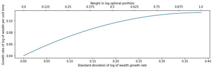
Figure 1: Efficient frontier for GBM without market impact.

In terms of risk preference, we adopt the volatility of the change in log of wealth as a proxy measure of risk. From equation 18, we can see that the volatility of the portfolio will be in the form of:

$$\sum^{3}_{i=1}\sum^{3}_{j=1}w_{i}w_{j}\sigma_{i}\sigma_{j}\rho_{ij}$$ (22)

Therefore, if we include a constraint on the volatility, the Lagrangian function has the same form as in equation 20 except with a Lagrange multiplier for the last term. In this case, the efficient frontier, under the assumption of no market impact, can be formed by a linear combination of the optimal portfolio derived from solving equation 21 and cash. In other words, we can focus on finding the log optimal portfolio and use it to obtain any portfolio on the efficient frontier by taking a fraction of the weights as shown in 1. This is sometimes called a fractional Kelly strategy [23].

4.2 GBM with market impact

The inclusion of market impact should cause the optimal policy to change. We note that the optimal policy is the same when $\eta$ and $\gamma$, which control the market impact, are set to 0. Therefore, when market impact is low, the optimal policy is close to the one without market impact. If each period is sufficiently short, the change in prices inter-period would be small which results in small adjustments to the portfolio, and hence low market impact.

The exception is the start of the episode when the portfolio is all cash and large adjustments have to be made to bring the portfolio to the desired weights. If the initial wealth is large, then this initial portfolio building phase can inccur a large cost. One way to mitigate this is to gradually adjust the portfolio weights to the required weights over the first $n$ periods. If $n$ is small relative to the episode length, then the resulting accumulated reward would be close to the optimal level without market impact.

Therefore, we can use the same optimal policy as the one without market impact as a baseline when the initial wealth is low. When the initial wealth is high, we slightly modify the baseline by staggering the initial portfolio build up.

4.3 Regime switching with market impact

With the regime switching model, the optimal weights in each regime can be very different which results in large adjustments to the portfolio. Under low wealth scenarios, gradually adjusting the portfolio weights to the required weights over the first $n$ periods was still sufficient to get close to the optimal growth rate without market impact. However, it was found to be insufficient under high wealth scenarios, producing extremely suboptimal growth rates. In fact, a high rate of bankruptcies were observed without a sufficiently long adjustment period. There are two reasons for this. Firstly, the adjustments can now happen multiple times within an episode. This causes costs to accumulate and the number of periods which the portfolio have suboptimal weights, due to the gradual adjustment, increases. Secondly, the difference in weights between a bullish and bearish regime is far larger than the difference between an all cash portfolio and single regime optimal weights.

To mitigate this, we observe that the efficient frontier in each regime also consists of a linear combination of the optimal weights in that regime and cash. A heuristically derived policy where a fraction of the optimal weights, in combination with gradual adjustments was used. A grid search on the fraction and adjustment period was performed to find the baseline policy. The performance of this policy is described in section 6.3.2.

5 Algorithms

The following algorithms will be tested:

1. Advantage actor critic (A2C) [24]

2. Deep deterministic policy gradients (DDPG) [25]

3. Proximal policy optimisation (PPO) [26]

4. Soft actor critic (SAC) [27]

5. Twin delayed deep deterministic policy gradients (TD3) [28]

All 5 algorithms are actor critic methods. DDPG, TD3 and SAC are off-policy algorithms that use Q-learning [29] to learn the action-value function from data that can include transitions not collected from the current policy. However, since the learned Q function is represented by a neural network, we cannot perform a simple argmax to find the optimal action. The differentiabilty of the Q function is exploited to use gradient ascent and update the policy, which is also a neural network, and maximise the Q value. One key difference between these methods is that SAC uses a stochastic policy while both DDPG and TD3 use deterministic policies. TD3 is an improvement on DDPG with adjustments made to address function approximation errors resulting from the use of neural networks.

A2C and PPO are on-policy algorithms with stochastic policies and use generalised advantage estimation (GAE) to compute the policy gradient. As the data is only used once to update the policy, the on-policy algorithms are usually less data efficient than off-policy algorithms. The use of the advantage function to reduce the variance of policy gradient estimators is well known in the literature [30]. GAE extends this by using an exponentially weighted average of multi-step advantages, which allows control over the bias variance trade off. PPO has two variants of which we focus on the clipping variant. This variant uses a heuristic to limit the change in the policy after each update. This introduces stability to the training process and reduces the likelihood of policy collapse.

The choice of the algorithms are motivated by their popularity in the literature and their ability to solve continuous control problems. The implementations from the Stable Baselines 3 library [31] were used for experiments.

6 Experiments

6.1 Low initial wealth

We consider experiments with low initial wealth of 1,000 which results in low market impact. The parameters for the GBM, market impact and algorithms are provided in appendix C. In this setting, the market impact is low and we expect the optimal policy to be close that described in section 4.1. There are 4 key findings in this set of experiments:

1. The use of GAE to tune the right trade-off between bias and variance has a strong influence on the result.

2. The clipping function of PPO reduces the likelihood of deviating from the optimal policy once it is found.

3. Off-policy algorithms were unable to learn a good policy due to an inability to learn the right Q function, which is likely caused by noise from the rewards.

4. It takes at least 2m steps with the best algorithm (PPO) to converge to a good policy

6.1.1 Generalised advantage estimation

The inherent stochasticity of the rewards causes high variance in the policy gradient. GAE allows tuning of the bias variance trade-off by exponential weighting ($\lambda$) of multi-step advantages.

Table 1: Evaluation of trained PPO agent over 10 runs with different values of $\lambda$

	agent growth rate		bankruptcies	baseline growth rate
$\lambda$	mean	MAD	mean	mean	MAD
0.00	-0.388	0.494	1.3	0.115	0.001
0.25	-0.062	0.128	0.1	0.113	0.004
0.50	0.052	0.033	0.0	0.114	0.004
0.75	0.081	0.023	0.0	0.112	0.002
0.80	0.100	0.015	0.0	0.115	0.005
0.85	0.100	0.011	0.0	0.112	0.004
0.90	0.100	0.009	0.0	0.115	0.007
0.95	0.082	0.017	0.0	0.113	0.004
1.00	0.079	0.014	0.0	0.112	0.004

Table 1 shows the results from evaluating a trained PPO agent. The objective is the log of final wealth divided by the initial wealth. We divided this by the time horizon, which is equivalent to a per unit time growth rate shown as the mean growth rate. The baseline policy consistently produces results close to the theorectical optimal of 0.114. Any episode that results in bankruptcy is removed from the calculation as the growth rate is undefined. The number of bankruptcies and the mean absolute deviation (MAD) of the growth rate is also shown. Results for A2C are in appendix A.

When a single step advantage ($\lambda=0$) is used, the agent is unable to learn a good policy. This is likely to due to high bias, compounded by noisy rewards. When the advantage is a Monte Carlo estimate ($\lambda=1$), the agent is able to learn a good policy. However, the performance is much stronger when $\lambda$ is between 0.8 and 0.9 which suggests an appropriate trade-off is required to manage the noisy rewards.

Even with the best value of $\lambda$, there remains a gap to the optimal growth rate. This is likely due to 3 factors:

1. The use stochastic optimisation which is inherently noisy.

2. The added noise from the rewards.

3. The flatness of the optimisation landscape near the optimal growth rate.

The last point is partly visualised in a simplier setting of two stocks in figure 3(a).

6.1.2 Clipping function of PPO

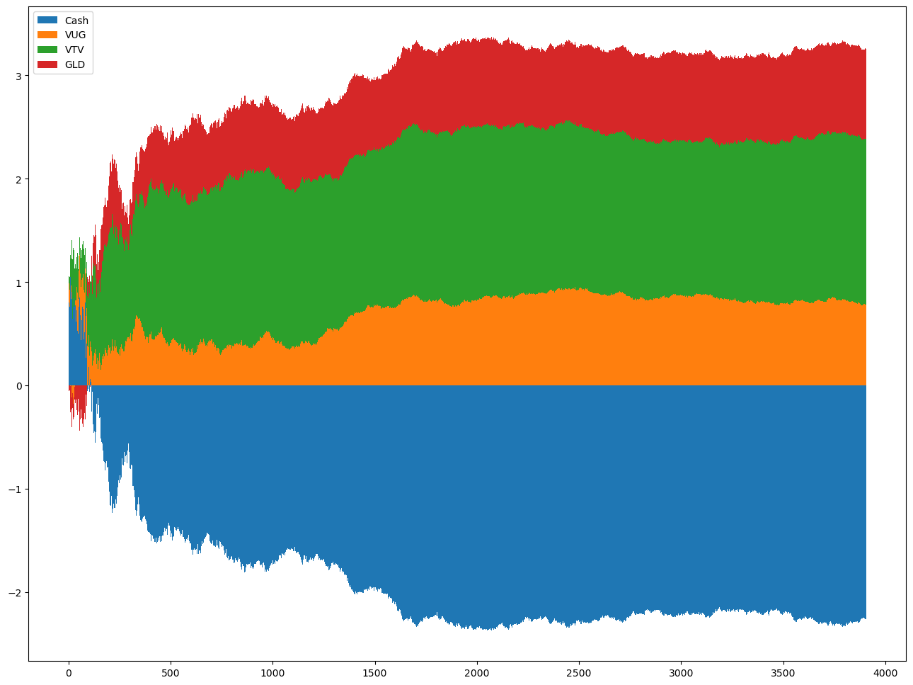
(a) Weights with clipping

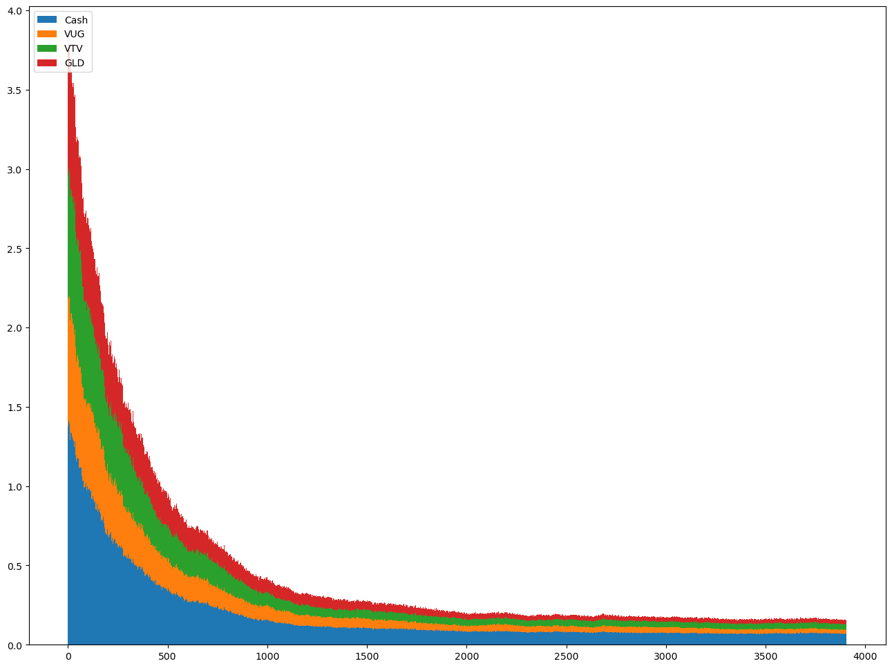
(b) MAD of weights in 2(a)

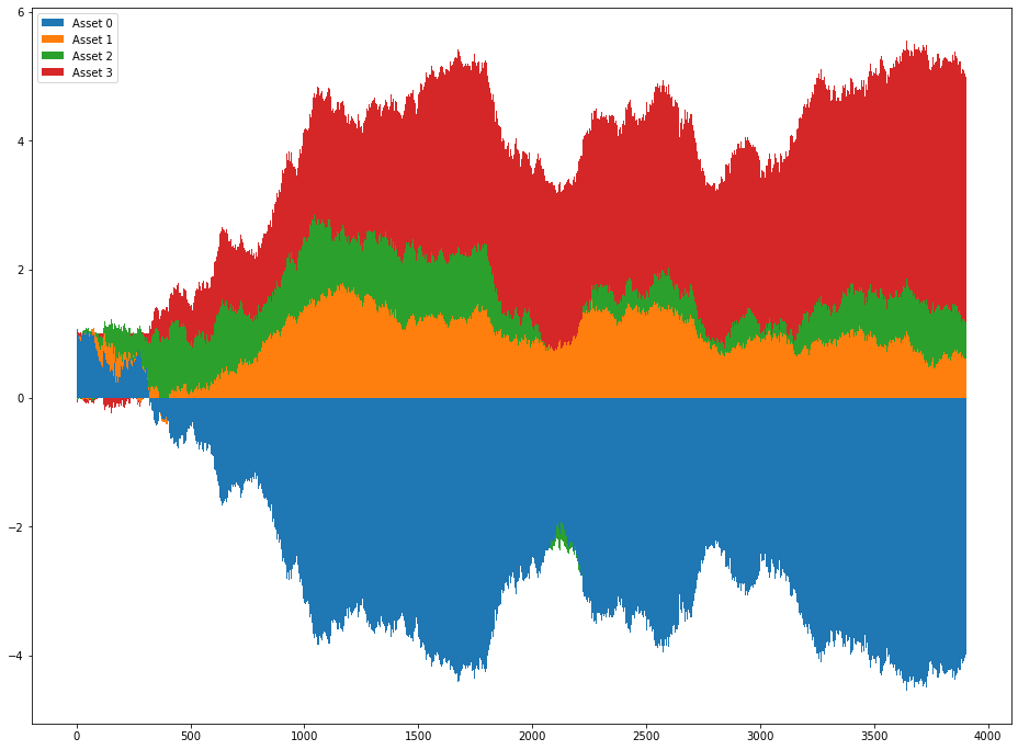
(c) Weights without clipping

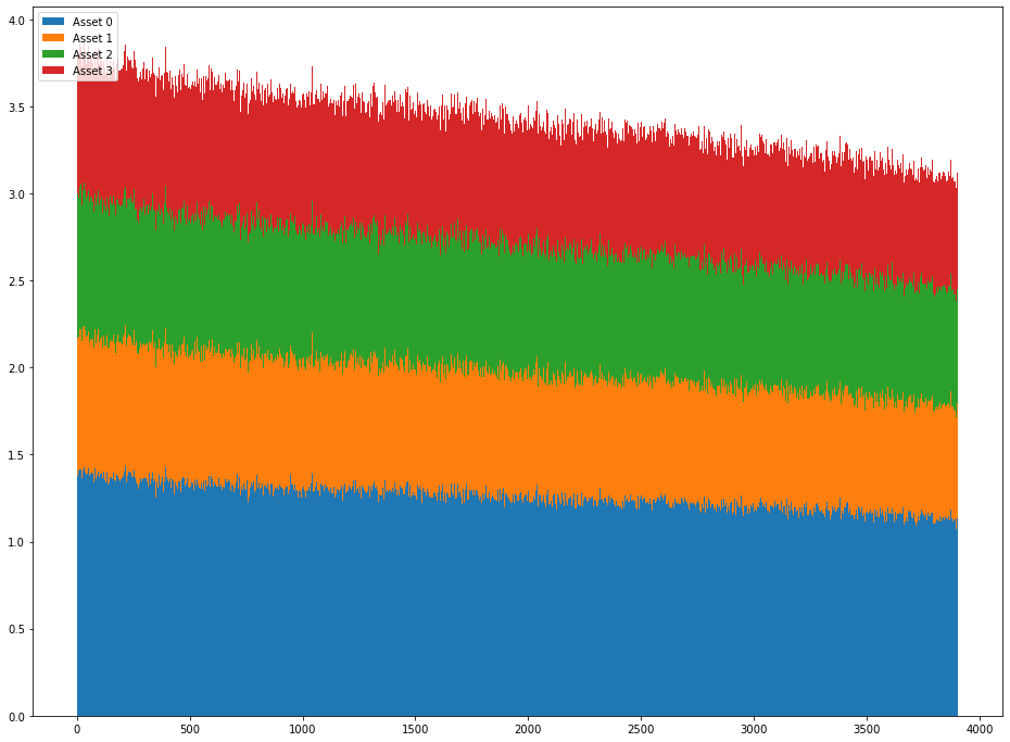
(d) MAD of weights in 2(c)

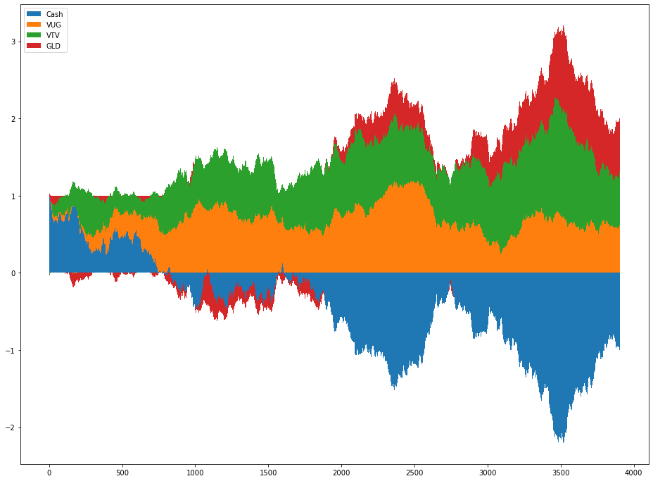
(e) Weights with A2C

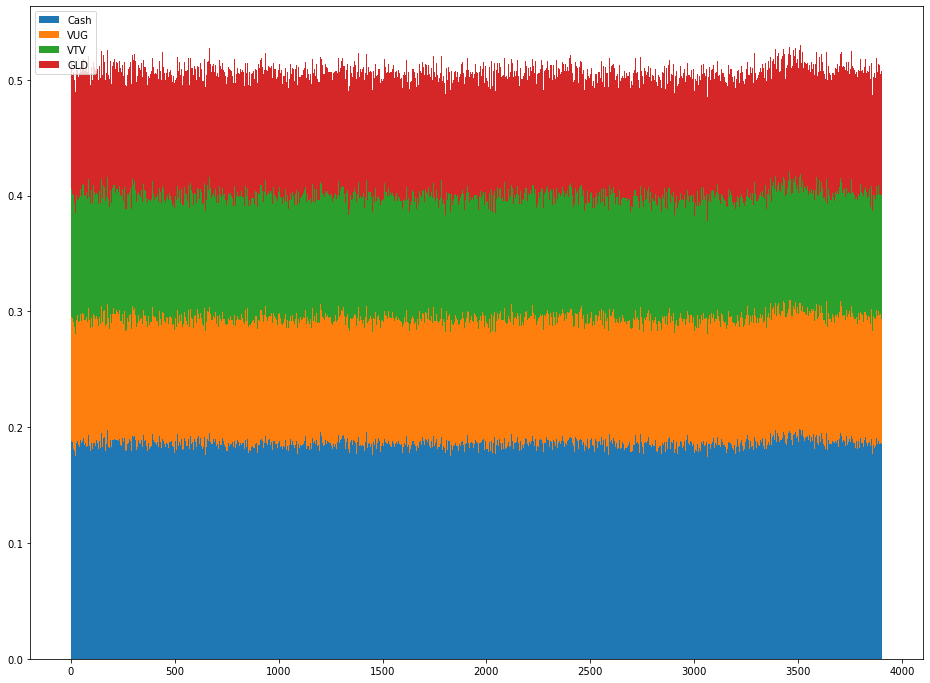
(f) MAD of weights in 2(e)

Figure 2: Importance of the clipping function in PPO

The clipping function on the probability ratios of the new over old policy is a key component of PPO. In the current setting, it was found to be important in preventing deviations from the optimal policy once it was found. Figure 2(a) is a stacked bar chart showing the evolution of average portfolio weights in an episode from a sample training run of PPO with clipping. Each point on the x-axis represents an episode and the y-axis represents the value of the portfolio weight. The baseline optimal weights are $[-1.72,0.76,0.66,1.31]$ for cash (blue), VUG (orange), VTV (green) and GLD (red) respectively. The key observation is that the weights stablises typically after 2,000 episodes of training. The clipped PPO agent successful learns that the optimal policy has fixed weights as confirmed by figure 2(b), which shows the corresponding evolution of the MAD of the weights within an episode.

The contrast when turning off the clipping or with A2C can be seen in figure 2(c) and 2(e) respectively. A2C is unable to converge towards a fixed weight policy asymptotically as seen in the unchanging MAD of weights in 2(f). Note that one difference with A2C was the initial log standard deviation of the Gaussian policy had to be set much lower for the algorithm to converge. For PPO without clipping, there was a trend towards lower MAD in the weights but the speed of convergence was orders of magnitude slower as seen in 2(d). Note that without clipping, it was necessary to train only a single epoch per update to prevent instability.

6.1.3 Difficulty of Q learning with noisy rewards

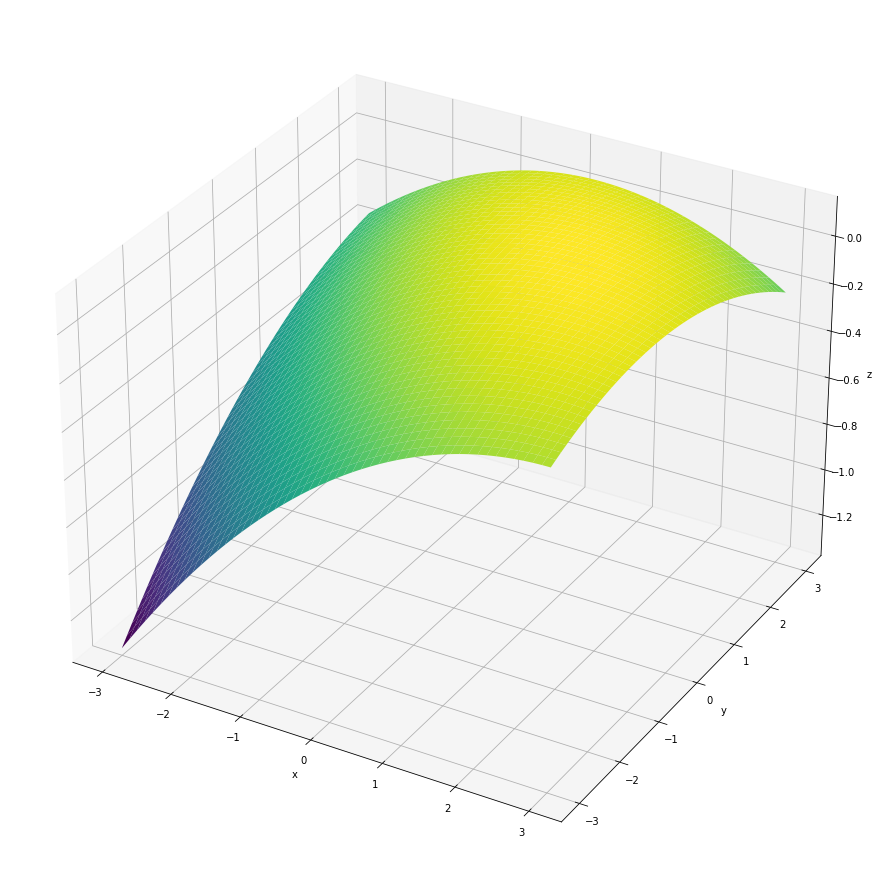
(a) Ground truth

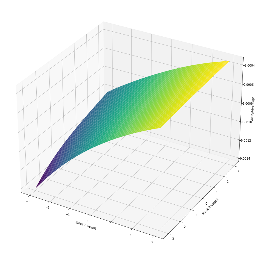
(b) DDPG critic

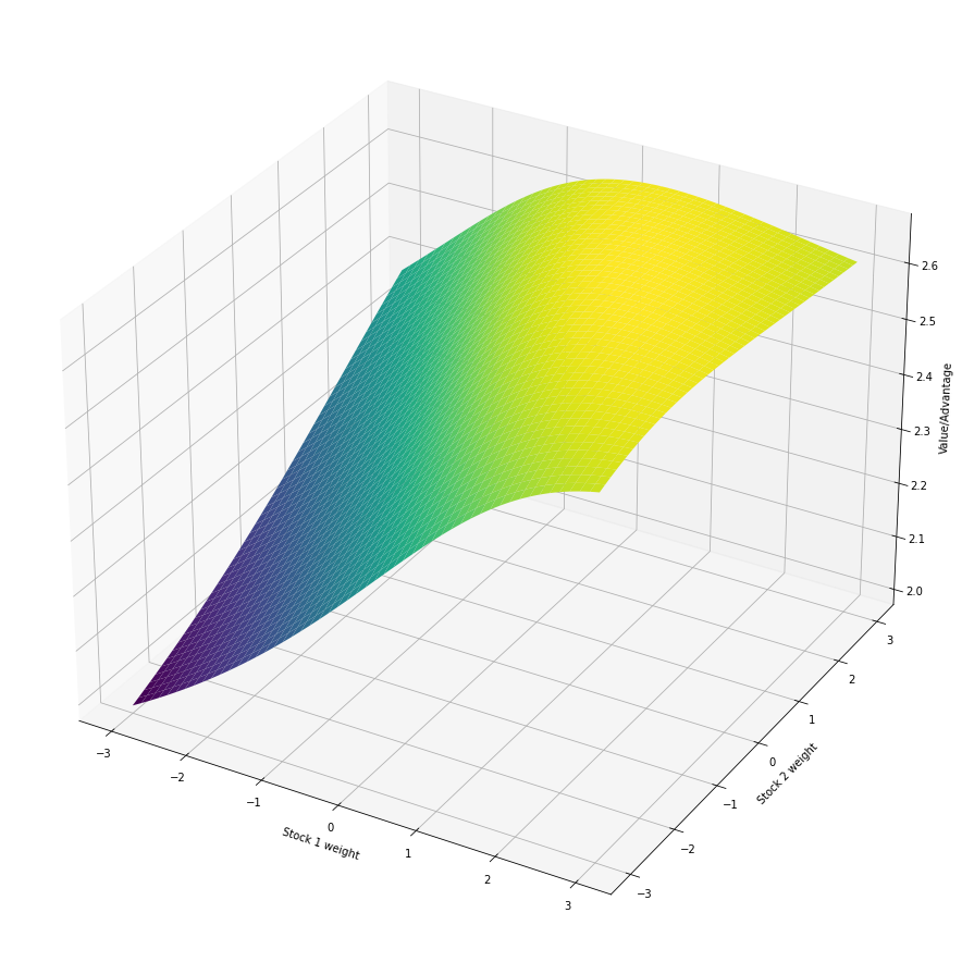
(c) Ground truth rewards

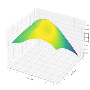
(d) $\beta$-NLL loss

Figure 3: Learning the Q function

The failure of the off-policy algorithms can be attributed to the noisy rewards received by the agent. A simplified experiment is conducted to investigate the difficulty of Q-learning in this noisy setting. We reduce the action space to two stocks to visualise the Q function. Figure 3(a) shows the ground truth for the Q function assuming zero market impact, which is independent of the state. When the wealth of the agent is low, we would expect the Q function in the environment with market impact to be similar.

Figure 3(b) shows the Q function learned by the DDPG agent with low wealth after more than 10m steps. The inability to learn the correct Q function can be attributed to noise. Figure 3(c) shows the DDPG critic when the noisy rewards were replaced with expected rewards. The algorithm successfully converges to a good policy when the rewards are noise free. Attempts to remedy the problem by increasing the size of the critic network or using a critic with a $\beta$-NLL loss [32] to learn a probabilistic Q function as shown in figure 3(d) were unsuccessful.

6.1.4 Sample efficiency

As PPO was found to be the best performing algorithm, we investigate the sample efficiency of the algorithm. Using tuned hyperparameters, we evaluate the growth rates of trained policies after increasing amount of training time steps. The results are shown in table 2.

Table 2: Sample efficiency of the algorithms

	agent growth rate		bankruptcies
time steps	mean	MAD	mean
100k	-0.133	0.013	0.0
500k	0.010	0.013	0.0
1m	0.065	0.019	0.0
2m	0.090	0.008	0.0
3m	0.091	0.010	0.0
4m	0.104	0.005	0.0
5m	0.100	0.009	0.0

PPO takes at least 2m time steps to converge to a sufficiently well performing policy. Note that if we take each period to represent a trading day, then 2m time steps corresponds to almost 8,000 years of training. This is far too inefficient considering the amount of data that is typically available in financial markets.

6.2 High initial wealth

When we increase the initial wealth of the agent, the effect of market impact becomes more pronounced. The baseline optimal policy derived in section 4.2 is able to attain similar performance as in the low wealth scenario i.e. mean growth rate of 0.114. Since PPO was the best performing algorithm in the low wealth scenario, we only compare the performance of PPO with the baseline policy in the high wealth scenario.

Table 3: Performance of PPO with different initial wealth

	agent growth rate		bankruptcies
wealth	mean	MAD	mean
100k	0.085	0.010	0.0
150k	0.082	0.005	0.0
200k	0.061	0.012	0.0
250k	0.043	0.032	0.0
300k	0.045	0.023	0.5

It was found that PPO was converging towards policies that produces weights approaching fractions of the optimal weights akin to a fractional Kelly strategy [23]. This lowers the cost of market impact but results in lower growth rates as seen in table 3. Attempts to have the agent learn the gradual adjustment behaviour such as with larger networks, use of a recurrent neural network architecture and use of CRL [19] were unsuccessful.

6.3 Regime switching model

For the regime switching model, we use the dual regime parameters estimated from [17] with a slight adjustment to prevent unrealistic levels of leverage as detailed in appendix D. There are also 3 stocks in this model representing, US, Germany and UK markets. The optimal weights, assuming no market impact, for each regime are as follows.

1. Bullish regime: $[-1.72,0.76,0.66,1.31]$ with an expected growth rate of 0.274

2. Bearish regime: $[1.56,-2.18,1.22,0.40]$ with an expected growth rate of 0.104

Based on the limiting distribution of the Markov chain, the expected growth rate of a policy that switches between these two sets of weights is 0.232 when there is no or low market impact.

When PPO is applied to this setting without modification, it is found to converge to the optimal fixed weight policy. In other words, it finds a set of fixed weights that is used for both regimes with the highest expected growth rate.

A modification, as mentioned in section 3.1.3, is required for the agent to learn a switching policy adapted to each regime. A multivariate Gaussian HMM is trained on the historical log returns, derived from the state, to infer the regime index. This serves as an additional context variable used in the network architecture shown in figure 4. The architecture used for the previous experiments is encased in the red box. The additional context network takes in the learned regime, $\hat{Z}_{t}$, and outputs a vector of the same size as the output of the feature net. These two are combined by element wise multiplication and fed into subsequent layers. More details are in appendix D.

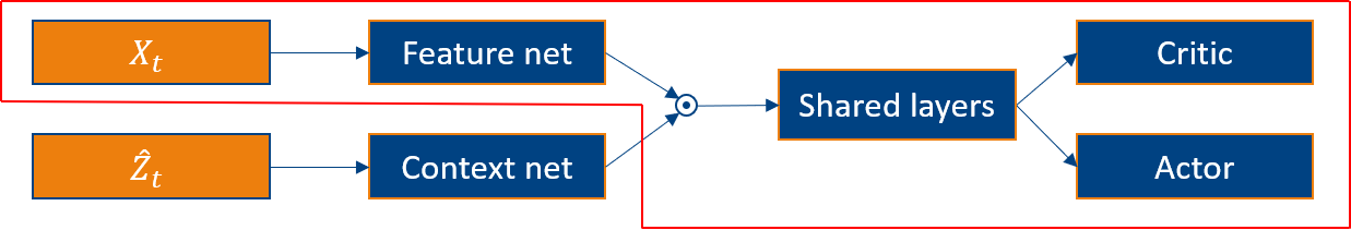
Figure 4: Network architecture for the regime switching model

6.3.1 Low initial wealth under regime switching model

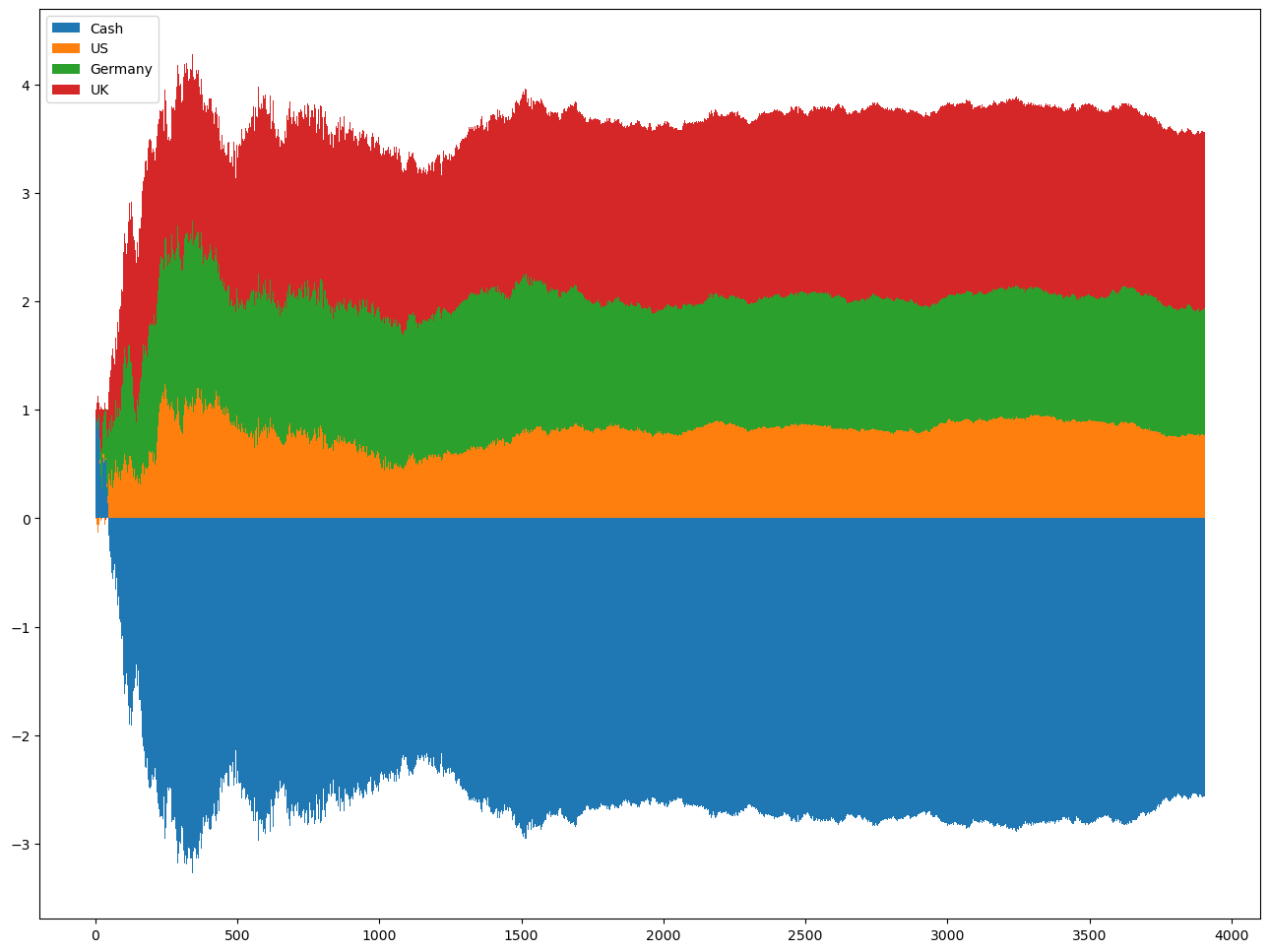
(a) Bullish regime weights

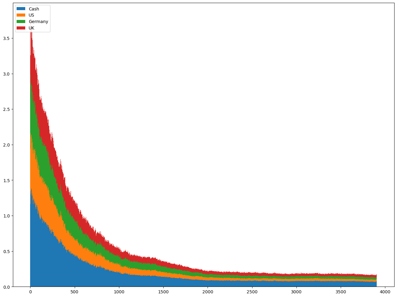
(b) MAD of weights in 5(a)

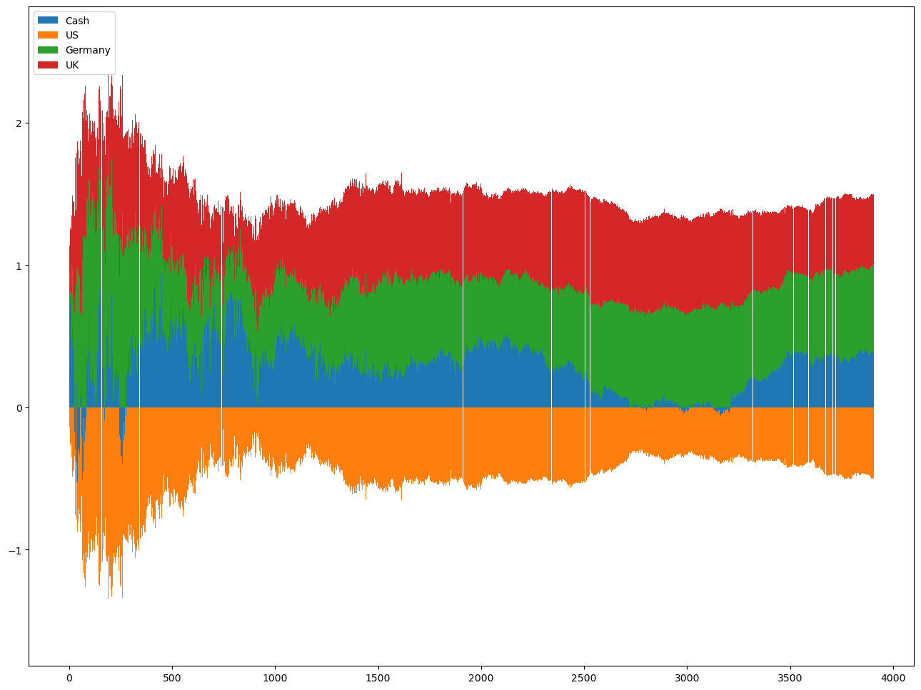
(c) Bearish regime weights

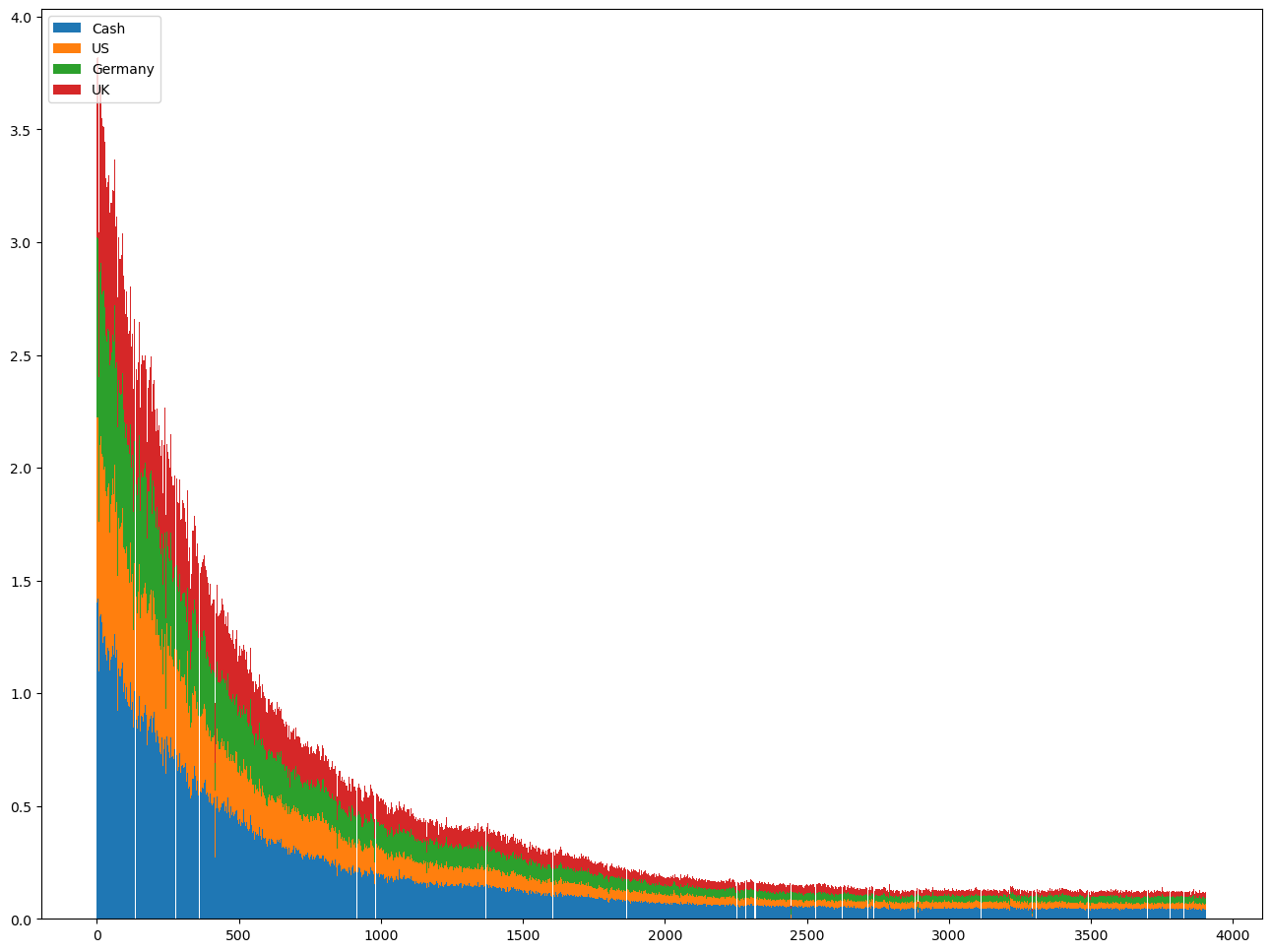
(d) MAD of weights in 5(c)

Figure 5: PPO with context on the regime switching model with low wealth

We see in figure 5 the same type of charts as described for 2. The key observation here is that the agent is now able to adapt different policies based on the predicted regime. Figure 5(a) and 5(c) show the weights of the stocks in the bullish and bearish regimes respectively. In particular, the agent has learned to reduce exposure and also short the US market in the bearish regime, consistent with the optimal policy. The agent also correctly learns that each regime’s optimal policy is still a fixed weight policy. Figure 5(b) and 5(d) show that it is converging towards fixed weights.

Over 10 runs, the agent achieves a mean growth rate of 0.161 with a MAD of 0.019. There are a few reasons that contribute to the wider gap from the optimal growth rate beyond those discussed in section 6.1.1. Firstly, a regime switch happens for at least one period before the HMM is able to predict the change and the agent is able to adapt compared to the foresight used in the baseline. Although it is an unfair comparison, we use foresight in the baseline as it provides a more accurate check on correctness when compared to the theorectical optimal. Secondly, while the HMM is able to predict the regime with a high accuracy of 0.971 on average, there is still an error rate which contributes to a dip in the growth rate. Overall, we see that the agent is able to learn the right attributes of the optimal policy.

6.3.2 High initial wealth under regime switching model

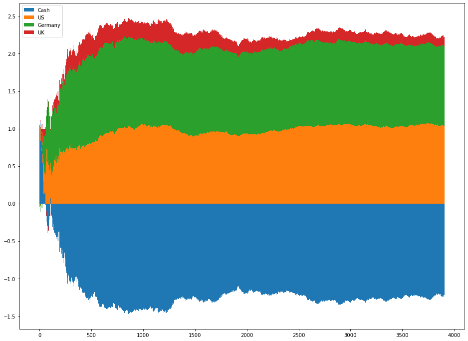
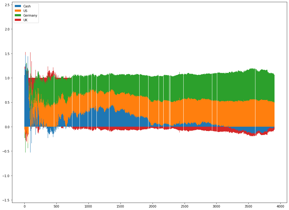
(a) Policy with distinct weights for each regime

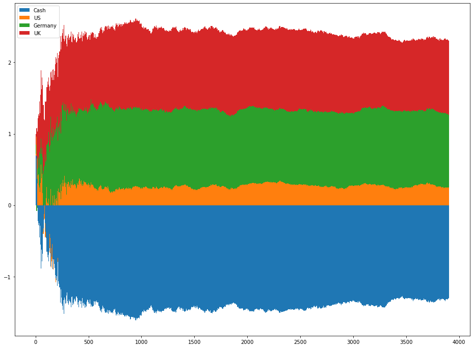
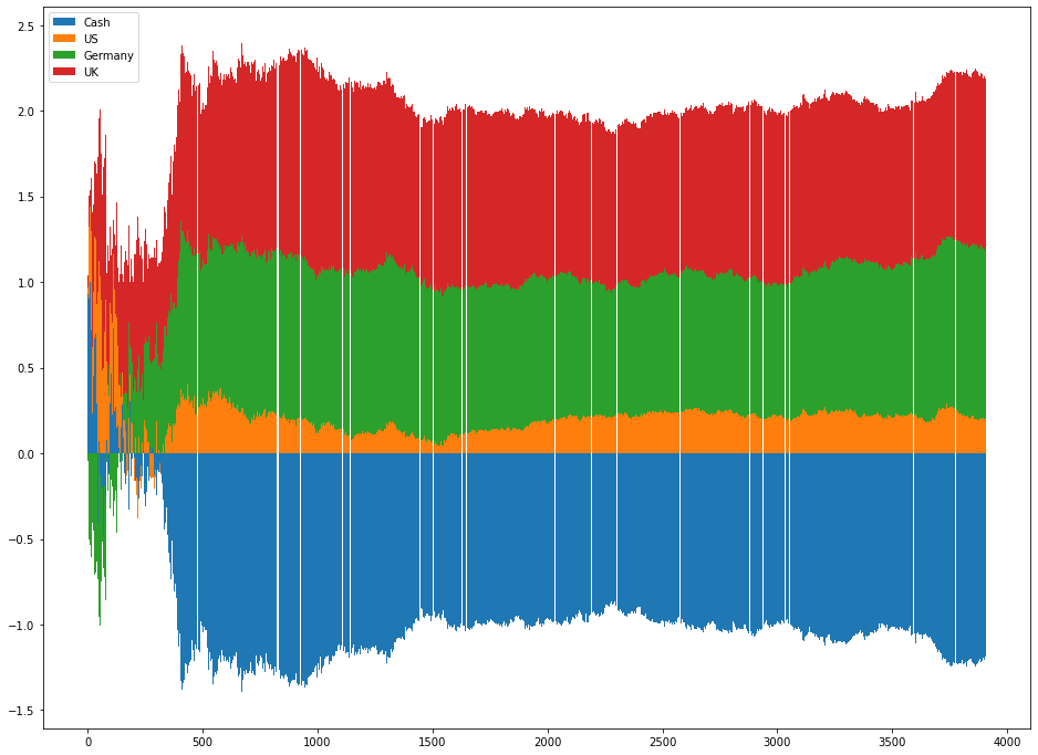
(b) Policy with similar weights for each regime

Figure 6: PPO with context on the regime switching model with high wealth

As discussed in section 4.3, the heuristically derived policy is used as the baseline. Under the higher wealth conditions set for this set of experiments, it achieves a mean growth rate of 0.164 with MAD of 0.004.

The PPO+HMM agent’s results are mixed across multiple runs with a mean growth rate of 0.088 and MAD of 0.016. The common thread across all runs is that the agent seeks policies akin to the fractional Kelly strategy seen in section 6.2 to limit the cost of market impact for each regime. In some cases, the policy converges towards more distinct policies for each regime as shown in figure 6(a) which achieved a growth rate of 0.091 In others, the policy has similar weights for both regimes as shown in figure 6(b) resulting in low costs and achieved a growth rate of 0.129. Overall, there is higher variance in the resulting policies as higher market impact costs delivers more noise into the rewards.

7 Conclusion

The common benckmark DRL algorithms were evaluated in the task of portfolio optimisation under a simulator based on geometric Brownian motion with the Bertsimas-Lo market impact model. The optimal policy under no market impact can be derived analytically and serves as an upper bound when market impact is included. This provides the baseline to evaluate the performances of the algorithms.

Due to the noisy nature of the problem, off-policy methods using Q-learning struggled to learn a good policy. The on-policy methods used generalised advantage estimation to reduce the variance in the policy gradient estimator and successfully converged to a close to optimal policy. Among the two on-policy methods, PPO’s clipping function was found to be more robust to the noise in terms of not drifting away once it had converged. In a more challenging and realistic setting of regime changes, we used a HMM to predict the regime and provide the appropriate context to the agent. This allowed the PPO algorithm to adapt different policies to each regime.

In all the cases, the sample efficiency is a limiting factor in the application of DRL to the problem of portfolio optimisation. With the best performing algorithm PPO and the simplest setting with low wealth and no regime changes, it took around 2m steps of training to learn a policy that is close to optimal. If we translate this into the number of trading days, it represents almost 8,000 years of data points. With financial data, we only see one realisation of the market with no option to reset the environment. Therefore, the results suggests large improvements on sample efficiency is required for successful application of DRL to the problem.

It is therefore not surprising that another avenue of research has emergered, which is to explore the use of autoencoders [33] or generative adversarial networks [34, 35] trained on real data to generate realistic synthetic data for training. As these are the early days of DRL in finance, and in particular portfolio optimisation, it remains to be seen how the field will develop and address these issues.

Appendix

Appendix A Experimental results for A2C

The same experimental setup as described in section C was used to evaluate A2C. The $\lambda$ parameter was varied and for each value, 10 runs were performed. Results are shown in the table below.

	agent growth rate		bankruptcies	baseline growth rate
$\lambda$	mean	MAD	mean	mean	MAD
0.00	-0.527	0.314	0.3	0.114	0.005
0.25	-0.061	0.176	0.2	0.111	0.004
0.50	0.023	0.075	0.0	0.112	0.005
0.75	0.082	0.010	0.0	0.115	0.004
0.90	0.089	0.008	0.0	0.111	0.006
0.95	0.087	0.010	0.0	0.116	0.006
1.00	0.065	0.029	0.0	0.118	0.005

Appendix B Common parameters for all experiments

The common parameters for all experiments are shown in the table below.

Variable	Value
T (Investment horizon)	5
Number of periods per unit of time	256
Number of periods in an episode	1280
$\eta$ (temporary impact factor)	1e-9
$\gamma$ (permanent impact factor)	1e-7
$l$ (historical window length)	60

Appendix C Experiment parameters for non-regime switching model

The interest rate for cash was set to 0.04. The GBM parameters are shown in the table below.

Table 4: Geometric Brownian motion parameters

Ticker	VUG	VTV	GLD
$\mu$ (drift)	0.124	0.105	0.072
$\sigma$ (volatility)	0.255	0.209	0.145
$\rho$ (correlation)	0.81/0.12	0.81/0.08	0.12/0.08

All experiments with non-regime switching model used 2 layers of 64 neurons in the feature extractor with a Tanh activation and 1 linear layer for the actor and critic. For the off-policy algorithms, various hyperparameters were tested but none successfully produced a policy that could consistently approach the baseline.

The hyperparameters for PPO are shown in table below.

Hyperparameter	Value
$\alpha$ (discount factor)	0.99
Learning rate	0.0003
Batch size	64
Num steps between updates	1280
Num epochs per update	10
Clip range	0.2
GAE $\lambda$	0.9 (unless otherwise specified)
Initial log std	0
Max grad norm	0.5
Value function loss coefficient	1.0
Entropy loss coefficient	0

The hyperparameters for A2C are shown in table below.

Hyperparameter	Value
$\alpha$ (discount factor)	0.99
Learning rate	0.0001
Batch size	256
Num steps between updates	256
Num gradient steps per update	1
GAE $\lambda$	0.9 (unless otherwise specified)
Initial log std	-2.0
Value function loss coefficient	1.0

Appendix D Experiment parameters for regime switching model

The interest rate for cash was set to 0.05 for the bull regime and 0.01 for the bear regime. The GBM parameters for the regime switching model are shown in table below. The growth rate for the US market was adjusted down as the original level was higher than both the Germany and UK market. Since it also had lower volatility than those markets, it resulted in optimal portfolio weights that were extremely skewed towards the US market with unrealistic leverage.

Regime	Parameter	US	Germany	UK
Bull	$\mu$ (drift)	0.103	0.138	0.140
Bull	$\sigma$ (volatility)	0.120	0.166	0.166
Bull	$\rho$ (correlation)	0.41/0.26	0.41/0.43	0.26/0.43
Bear	$\mu$ (drift)	-0.021	0.097	0.042
Bear	$\sigma$ (volatility)	0.216	0.379	0.288
Bear	$\rho$ (correlation)	0.60/0.45	0.60/0.45	0.45/0.45

The per period transitional probabilities of the Markov chain are shown in the table below. The original probabilities were estimated from [17] were estimated for monthly returns. We rescale them using equation 14 to daily returns which are closer to the setting of the experiment. Specifically, we solve for the infinitesimal generator matrix $Q$ where $e^{\frac{1}{12}Q}$ equals the parameters in [17]. Then we get the required probabilities by computing $e^{\frac{1}{256}Q}$.

Regime	$P(Bull|Regime)$	$P(Bear|Regime)$
Bull	0.997	0.003
Bear	0.009	0.991

The structure of the neural network architecture is shown in the figure below. The feature net has 3 layers with 256, 128 and 64 neurons respectively and a Tanh activation function. The regime net has 3 layers with 64 neurons each and a ReLU activation function. The shared layers consists of 2 layers with 64 neurons each and a Tanh activation function. The actor and critic each have a single linear layer.

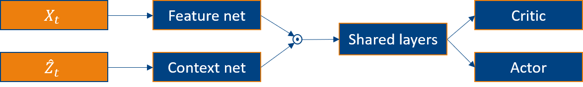
Figure 7: Network architecture for the regime switching model

The multivariate Gaussian HMM was trained using the Viterbi algorithm [20] implemented by hmmlearn (https://github.com/hmmlearn/hmmlearn). Due to the possibility of no bear regime appearing in a single episode, the HMM is trained for the first 10 episodes of each experimental run. Thereafter, the learned parameters are frozen. The hyperparameters for the algorithm are shown in the table below. Hyperparameters not shown are using default values.

Hyperparamter	Value
Number of components (regimes)	2
Number of initialisations	10
Max number of iterations per initialisation	100
Log likelihood convergence threshold	1e-7
Prior for mean	1e-4
Prior for covariance	1e-4
Min covariance value	1e-6

References

- [1] Leonard C MacLean, Edward O Thorp, and William T Ziemba. The Kelly capital growth investment criterion: Theory and practice, volume 3. world scientific, 2011.
- [2] Leonard C MacLean, Edward O Thorp, and William T Ziemba. Good and bad properties of the kelly criterion. Risk, 20(2):1, 2010.
- [3] John Moody and Matthew Saffell. Reinforcement learning for trading. Advances in Neural Information Processing Systems, 11:917–923, 1998.
- [4] John Moody, Lizhong Wu, Yuansong Liao, and Matthew Saffell. Performance functions and reinforcement learning for trading systems and portfolios. Journal of Forecasting, 17(5-6):441–470, 1998.
- [5] J. Moody and M. Saffell. Learning to trade via direct reinforcement. IEEE Transactions on Neural Networks, 12(4):875–889, 2001.
- [6] Zhengyao Jiang, Dixing Xu, and Jinjun Liang. A deep reinforcement learning framework for the financial portfolio management problem. arXiv pre-print server, 2017.
- [7] Zhuoran Xiong, Xiao-Yang Liu, Shan Zhong, Hongyang Yang, and Anwar Walid. Practical deep reinforcement learning approach for stock trading. arXiv pre-print server, 2018.
- [8] Yunan Ye, Hengzhi Pei, Boxin Wang, Pin-Yu Chen, Yada Zhu, Ju Xiao, and Bo Li. Reinforcement-learning based portfolio management with augmented asset movement prediction states. Proceedings of the AAAI Conference on Artificial Intelligence, 34(01):1112–1119, 2020.
- [9] Jingyuan Wang, Yang Zhang, Ke Tang, Junjie Wu, and Zhang Xiong. Alphastock. In Proceedings of the 25th ACM SIGKDD International Conference on Knowledge Discovery & Data Mining, pages 1900–1908, 2019.
- [10] Yue Deng, Feng Bao, Youyong Kong, Zhiquan Ren, and Qionghai Dai. Deep direct reinforcement learning for financial signal representation and trading. IEEE Transactions on Neural Networks and Learning Systems, 28(3):653–664, 2017.
- [11] Zihao Zhang, Stefan Zohren, and Stephen Roberts. Deep reinforcement learning for trading. The Journal of Financial Data Science, 2(2):25–40, 2020.
- [12] Ke Xu, Yifan Zhang, Deheng Ye, Peilin Zhao, and Mingkui Tan. Relation-aware transformer for portfolio policy learning. In Proceedings of the Twenty-Ninth International Conference on International Joint Conferences on Artificial Intelligence, pages 4647–4653, 2021.
- [13] Weiwei Shen, Jun Wang, Yu-Gang Jiang, and Hongyuan Zha. Portfolio choices with orthogonal bandit learning. In Proceedings of the 24th International Conference on Artificial Intelligence, pages 974–980 , numpages = 7. AAAI Press, 2015.
- [14] Matthew Dixon and Igor Halperin. G-learner and girl: Goal based wealth management with reinforcement learning. arXiv preprint arXiv:2002.10990, 2020.
- [15] Steven E Shreve. Stochastic Calculus for Finance. Springer, 2004.
- [16] Dimitris Bertsimas and Andrew W. Lo. Optimal control of execution costs. Journal of Financial Markets, 1(1):1–50, 1998.
- [17] Andrew Ang and Geert Bekaert. International asset allocation with regime shifts. The Review of Financial Studies, 15(4):1137–1187, 2002.
- [18] Huntley Schaller and Simon Van Norden. Regime switching in stock market returns. Applied Financial Economics, 7(2):177–191, 1997. doi: 10.1080/096031097333745.
- [19] Assaf Hallak, Dotan Di Castro, and Shie Mannor. Contextual markov decision processes. arXiv preprint arXiv:1502.02259, 2015.
- [20] Lawrence R Rabiner. A tutorial on hidden markov models and selected applications in speech recognition. Proceedings of the IEEE, 77(2):257–286, 1989.
- [21] Bogdan Doytchinov and Rachel Irby. Time discretization of markov chains. Pi Mu Epsilon Journal, 13(2):69–82, 2010.
- [22] Richard S Sutton and Andrew G Barto. Reinforcement learning: An introduction. MIT press, 2018.
- [23] Mark Davis and Sébastien Lleo. Fractional Kelly strategies for benchmarked asset management, pages 385–407. The Kelly Capital Growth Investment Criterion: Theory and Practice, 2011.
- [24] Yuhuai Wu, Elman Mansimov, Shun Liao, Alec Radford, and John Schulman. Openai baselines: Acktr & a2c, 2017.
- [25] Timothy P Lillicrap, Jonathan J Hunt, Alexander Pritzel, Nicolas Heess, Tom Erez, Yuval Tassa, David Silver, and Daan Wierstra. Continuous control with deep reinforcement learning. In International Conference on Learning Representations, 2016.
- [26] John Schulman, Filip Wolski, Prafulla Dhariwal, Alec Radford, and Oleg Klimov. Proximal policy optimization algorithms. arXiv preprint arXiv:1707.06347, 2017.
- [27] Tuomas Haarnoja, Aurick Zhou, Pieter Abbeel, and Sergey Levine. Soft actor-critic: Off-policy maximum entropy deep reinforcement learning with a stochastic actor. In Proceedings of the 35th International Conference on Machine Learning, volume 80, pages 1861–1870. PMLR, 2018.
- [28] Scott Fujimoto, Herke Hoof, and David Meger. Addressing function approximation error in actor-critic methods. In International Conference on Machine Learning, pages 1587–1596. PMLR, 2018.
- [29] Christopher J. C. H. Watkins and Peter Dayan. Q-learning. Machine Learning, 8(3):279–292, 1992.
- [30] Evan Greensmith, Peter L Bartlett, and Jonathan Baxter. Variance reduction techniques for gradient estimates in reinforcement learning. Journal of Machine Learning Research, 5(9), 2004.
- [31] Antonin Raffin, Ashley Hill, Adam Gleave, Anssi Kanervisto, Maximilian Ernestus, and Noah Dormann. Stable-baselines3: Reliable reinforcement learning implementations. Journal of Machine Learning Research, 22(268):1–8, 2021.
- [32] Maximilian Seitzer, Arash Tavakoli, Dimitrije Antic, and Georg Martius. On the pitfalls of heteroscedastic uncertainty estimation with probabilistic neural networks. In International Conference on Learning Representations, 2022.
- [33] Hans Buehler, Blanka Horvath, Terry Lyons, Imanol Perez Arribas, and Ben Wood. A data-driven market simulator for small data environments. arXiv preprint arXiv:2006.14498, 2020.
- [34] Magnus Wiese, Robert Knobloch, Ralf Korn, and Peter Kretschmer. Quant gans: deep generation of financial time series. Quantitative Finance, 20(9):1419–1440, 2020. doi: 10.1080/14697688.2020.1730426.
- [35] Adriano Koshiyama, Nick Firoozye, and Philip Treleaven. Generative adversarial networks for financial trading strategies fine-tuning and combination. Quantitative Finance, 21(5):797–813, 2021. doi: 10.1080/14697688.2020.1790635.