DIGEST: Fast and Communication Efficient Decentralized Learning with Local Updates

Abstract

Two widely considered decentralized learning algorithms are Gossip and random walk-based learning. Gossip algorithms (both synchronous and asynchronous versions) suffer from high communication cost, while random-walk based learning experiences increased convergence time. In this paper, we design a fast and communication-efficient asynchronous decentralized learning mechanism DIGEST by taking advantage of both Gossip and random-walk ideas, and focusing on stochastic gradient descent (SGD). DIGEST is an asynchronous decentralized algorithm building on local-SGD algorithms, which are originally designed for communication efficient centralized learning. We design both single-stream and multi-stream DIGEST, where the communication overhead may increase when the number of streams increases, and there is a convergence and communication overhead trade-off which can be leveraged. We analyze the convergence of single- and multi-stream DIGEST, and prove that both algorithms approach to the optimal solution asymptotically for both iid and non-iid data distributions. We evaluate the performance of single- and multi-stream DIGEST for logistic regression and a deep neural network ResNet20. The simulation results confirm that multi-stream DIGEST has nice convergence properties; i.e., its convergence time is better than or comparable to the baselines in iid setting, and outperforms the baselines in non-iid setting.

Machine learning, distributed learning, decentralized learning, local stochastic gradient descent (SGD), federated learning.

1 Introduction

Emerging applications such as Internet of Things (IoT), mobile healthcare, self-driving cars, etc. dictates learning be performed on data predominantly originating at edge and end user devices [1, 2, 3]. A growing body of research work, e.g., federated learning [4, 5, 6, 7, 8, 9] has focused on engaging the edge in the learning process, along with the cloud, by allowing the data to be processed locally instead of being shipped to the cloud. Learning beyond the cloud can be advantageous in terms of better utilization of network resources, delay reduction, and resiliency against cloud unavailability and catastrophic failures. However, the proposed solutions, like federated learning, predominantly suffer from having a critical centralized component referred to as the Parameter Server (PS) organizing and aggregating the devices’ computations. Decentralized learning, advocating the elimination of PSs, emerges as a promising solution to this problem.

Decentralized algorithms have been extensively studied in the literature, with Gossip algorithms receiving the lion’s share of research attention [10, 11, 12, 13, 14, 15, 16, 17]. In Gossip algorithms, each node (edge or end user device) has its own locally kept model on which it effectuates the learning by talking to its neighbors. This makes Gossip attractive from a failure-tolerance perspective. However, this comes at the expense of a high network resource utilization. As shown in Fig. 1(a), all nodes in a Gossip algorithm in a synchronous mode perform a model update and wait for receiving model updates from their neighbors. When a node completes receiving all the updates from its neighbors, it aggregates the updates. As seen, there should be data communication among all nodes after each model update, which is a significant synchronization overhead. Furthermore, some nodes may be a bottleneck for the synchronization as these nodes (which are also called stragglers) can be delayed due to computation and/or communication delays, which increases the convergence time.

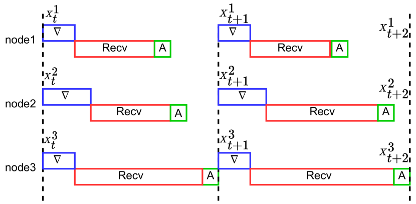
(a) Sync-Gossip

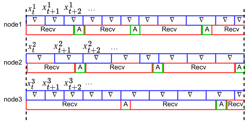
(b) Async-Gossip

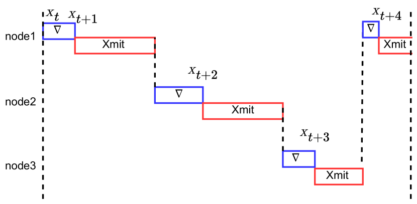
(c) Random-Walk

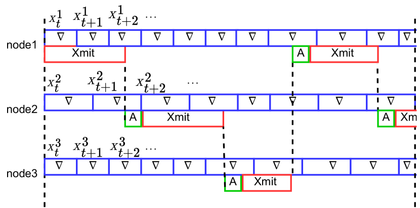
(d) DIGEST

Figure 1: DIGEST in perspective as compared to existing decentralized learning algorithms; (a) synchronous Gossip, asynchronous Gossip, and random-walk. Note that “$\nabla$” represents a model update. “Xmit” represents the transmission of a model from a node to one of its neighbors. “Recv” represents the communication duration while receiving model updates from all of a node’s neighbors. “A” represents model aggregation. $\mathbf{x}^{v}_{t}$ shows the local model of node $v$ at iteration $t$. For random walk algorithm, the global model iterates are denoted as $\mathbf{x}_{t}$.

Asynchronous Gossip algorithms, where nodes communicate asynchronously and without waiting for others are promising to reduce idle nodes and eliminate the stragglers, i.e., delayed nodes [18, 19, 20, 21]. Indeed, asynchronous algorithms significantly reduce the idle times of nodes by performing model updates and model exchanges simultaneously as illustrated in Fig. 1(b). For example, node 1 can still update its model from $\mathbf{x}_{t}^{1}$ to $\mathbf{x}_{t+1}^{1}$ and $\mathbf{x}_{t+2}^{1}$ while receiving model updates from its neighbors. When it receives from all (or some) of its neighbors, it performs model aggregation. However, nodes still rely on iterative Gossip averaging of their models, so updates propagate gradually across the network. Such delayed updates, also referred as gradient staleness in asynchronous Gossip may lead to high error floors [22], or require very strict assumptions to converge to the optimum solution [18]. Moreover, such methods must be implemented with caution to prevent the occurrence of deadlocks [19].

In both synchronous and asynchronous Gossip, models propagate over the nodes and updated by each node gradually as seen Fig. 2(a). This may lead to a notion that we name “diminishing updates”, where a node’s update (e.g., node 1 in Fig. 2(a)), even though crucial for convergence, may be averaged and mixed with other models in the next node (e.g., node 2 in Fig. 2(a)). The diminishing updates are more emphasized when a model passes through high degree nodes, and detrimental for the convergence in when data distribution heterogeneous across the nodes.

If Gossip algorithms are one side of the spectrum of decentralized learning algorithms, the other side is random-walk based decentralized learning [23, 24, 25, 26]. The random-walk algorithms advocate activating a node at a time, which would update the global model with its local data as illustrated in Fig. 1(c). Then, the node selects one of its neighbors randomly and sends the updated global model. The selected neighbor becomes a newly activated node, so it updates the global model using its local data. This continues until convergence. Random-walk algorithms reduce the communication cost as well as computation with the cost of increased convergence time due to idle times at nodes.

The goal of this work is to take advantage of both Gossip and random-walk ideas to design a fast and communication- efficient decentralized learning. Our key intuitions are; (i) Nodes do not need to communicate as much as Gossip to update their models, i.e., a sporadic exchange of model updates is sufficient; (ii) the diminishing updates inherent to Gossip algorithms can be eliminated by employing a global model (as shown in Fig. 2(b) and detailed in Section 3); and (iii) nodes do not need to wait idle as in random walk.

We design a fast and communication-efficient asynchronous decentralized learning mechanism DIGEST by particularly focusing on stochastic gradient descent (SGD). DIGEST is an asynchronous decentralized learning algorithm building on local-SGD algorithms, which are originally designed for communication efficient centralized learning [27, 28, 29]. In local-SGD, each node performs multiple model updates before sending the model to the PS. The PS aggregates the updates received from multiple nodes and transmits the updated global model back to nodes. The sporadic communication between nodes and the PS reduces the communication overhead. We exploit this idea for asynchronous decentralized learning. The following are our contributions.

• Design of DIGEST. We design a fast and communication-efficient asynchronous decentralized learning mechanism; DIGEST by particularly focusing on stochastic gradient descent (SGD). DIGEST works as follows. Each node keeps updating its local model all the time as in local-SGD. Meanwhile, there is an ongoing stream of global model update among nodes, Fig. 1(d). For example, node 1 starts transmitting the global model to node 2 at time $t$. When node 2 receives the global model from node 1, it aggregates it with its local model. The aggregated global model is transmitted to node 3 next. We note that the exchanged models are global models as each node adds its own local updates to the received model. A node that has the global model selects the next node randomly among its neighbors for global model transmission. After all the nodes update their models with a global model, DIGEST pauses global model exchange, while local SGD computations still continue. The global model exchange is repeated at every $H$ iterations. We name this algorithm single-stream DIGEST.

  (a) Gossip

  (b) DIGEST

  Figure 2: Spread of information across a decentralized network.

• Multi-Stream DIGEST. We further improve the convergence time of single-stream DIGEST by enabling multiple streams of global model updates. For example, there are $4$ streams working together at Fig. 3, where each stream operates on a smaller part of the network, so global model update can completed quickly. We identify the multiple streams using a rooted tree, which is determined in a decentralized manner via a distance vector algorithm [30]. Note that two or more streams may intersect at one node which is how the nodes aggregate their global models. The communication overhead may increase when the number of streams increases, and there is a nice convergence and communication overhead trade-off which can be exploited by adjusting $H$.

• Convergence analysis of DIGEST. We analyze the convergence of single- and multi-stream DIGEST, and prove that both algorithms approach to the optimal solution asymptotically. We show that DIGEST’s approach of simultaneous model updating and local SGD iterations do not hurt the convergence rate and do not create any convergence gap. Furthermore, multi-stream DIGEST is not affected by the network topology, i.e., even high degree nodes do not create any learning bias. We also indicate how frequently global model updates should be made, i.e., what the value of $H$ should be to achieve linear speed-up $O(\frac{1}{VT})$ in both iid and non-iid cases, where $V$ is the number of nodes in the network and $T$ is total number of iterations.

• Evaluation of DIGEST. We evaluate the performance of single- and multi-stream DIGEST for logistic regression and a deep neural network ResNet20 [31] for datasets w8a [32] and MNIST [33], and CIFAR-10 [34]. We consider both iid and non-iid data distributions over a various network topologies with different number of nodes. The simulation results confirm that DIGEST has nice convergence properties; i.e., its convergence time is better than or comparable to the baselines in iid setting, and outperforms the baselines in non-iid setting.

Figure 3: Example multi-stream DIGEST.

2 Related Work

Decentralized optimization algorithms have been widely studied in the literature, where nodes interact with their neighbors to solve an optimization problem [35, 36, 37, 38]. Despite their potential, these algorithms suffer from a bias in non-iid data [39], and they require synchronization and orchestration among nodes, which is costly in terms of communication overhead.

Decentralized algorithms based on Gossip involves a mixing step where nodes compute their new models by mixing their own and neighbors’ models [40, 41, 16]. However, this is costly in terms communication as every node requires $O(\deg(G))$ data exchange for every model update for a graph $G$. Furthermore, model updates propagate gradually over the network due to iterative gossip averaging. Such gradual model propagation reduces the convergence time and makes the learning mechanism very sensitive to data distribution over nodes. Finally, Gossip algorithms tend to favor higher-degree nodes while updating models, which causes slower convergence for non-iid data [42]. Our goal in this paper is to reduce the communication cost in decentralized learning for any data distribution without hurting convergence.

Asynchronous Gossip algorithms are designed to improve synchronous Gossip algorithms. The main focus of asynchronous Gossip is the reduction of synchronization costs in a gossip setting by utilizing non-blocking communication [18, 19, 43]. This means that nodes could potentially receive and use the stale versions of neighboring nodes’ models to update their own models. Despite this modification asynchronous Gossip algorithms continue to rely on the traditional Gossip to spread the information, where each nodes sends its model to all of its neighbors, which still introduces high communication cost. Our goal in this paper is to reduce the communication cost in an asynchronous manner for decentralized learning.

A random walk-based decentralized learning is considered in [24], which is similar to work on random walk data sampling for stochastic gradient descent, e.g., [25, 26]. Reducing the global averaging rounds as compared to Gossip-based mechanisms is considered in [44] by one-shot averaging. However, the global averaging rounds require long synchronization duration for large networks, which increases the convergence time. Also, only iid data is considered [44]. As compared to Gossip and random walk-based algorithms, DIGEST designs a communication efficient decentralized learning without hurting convergence rate for both iid and non-iid data.

3 Design of DIGEST

3.1 Preliminaries

Network Topology. We model the underlying network topology with a connected graph $G=(\mathcal{V},\mathcal{E})$, where $\mathcal{V}$ is the set of vertices (nodes) and $\mathcal{E}$ is the set edges. The vertex set contains $V$ nodes, i.e., $|\mathcal{V}|=V$, and $|.|$ shows the size of the set. The computing capabilities of nodes are arbitrary and heterogeneous. If node $i$ is connected to node $j$ through a communication link and can transmit data, then link $\{i,j\}$ is in the edge set, i.e., $\{i,j\}\in\mathcal{E}$. The set of the nodes that node $i$ is connected to and can transmit data is called the neighbors of node $i$, and the neighbor set of node $i$ is denoted by $\mathcal{N}_{i}$. We do not make any assumptions about the behavior of the communication links; there can be an arbitrary, but finite amount of delay over the links.

Data. We consider a setup where nodes have access to a subset of data samples $\mathcal{D}$. Each node $v$ has a local dataset $\mathcal{D}_{v}$, where $D_{v}=|\mathcal{D}_{v}|$ is the size of the local dataset and $D=\sum_{v=1}^{V}D_{v}$. The distribution of data across nodes is not identical and independently distributed (non-iid).

Stochastic Optimization. Assume that the nodes in the network jointly minimize a $d$-dimensional function $f:\mathbb{R}^{d}\rightarrow\mathbb{R}$. The goal of the nodes is to converge on a model $\mathbf{x}^{*}$, which minimizes the empirical loss over $D$ samples, i.e., $\mathbf{x}^{*}:=\arg\min_{\mathbf{x}\in\mathbb{R}^{d}}\Big{[}f(\mathbf{x}):=\frac{1}{D}\sum_{i=1}^{D}f_{i}(\mathbf{x})\Big{]}$, where $f_{i}(\mathbf{x}):\mathbb{R}^{d}\rightarrow\mathbb{R}$ is the loss function of $\mathbf{x}$ associated with the data sample $i$. The optimum solution is denoted by $f^{*}$. The loss function on local dataset $\mathcal{D}_{v}$ at node $v$ is $f^{v}(\mathbf{x})=\frac{1}{D_{v}}\sum_{i\in\mathcal{D}_{v}}f_{i}(\mathbf{x})$.

Notation. We provide our notation table in Appendix .1.

3.2 Single-Stream DIGEST

3.2.1 Overview

Local Model Update. We assume that the time is slotted, and at each slot/iteration, a local model is updated. However, a calculation of a gradient may take more than one slot, vary over time, or not fit into slot boundaries. Thus, at each iteration $t$, any gradients which have been delayed up to iteration $t$, and not used in previous local updates are used to update the local model. We note that time slots across nodes do not need to be synchronized in DIGEST as each node can have its own iteration sequence and update local and global models over its own sequence. The only assumption we make is that the slot sizes are the same across nodes, which can be decided a priori.

Let us consider that ${L}^{v}_{T}=\{l^{v}_{t}\}_{0\leq t<T}$ is the set of the delayed gradient calculations at node $v$, where $l^{v}_{t}$ shows that the local-SGD update of iteration $t$ is delayed until iteration $l^{v}_{t}$. For instance, $l^{v}_{t^{\prime}}=t$ means that the local-SGD of iteration $t^{\prime}$ is lagged behind and performed in iteration $t$, $t\geq t^{\prime}$. Then, we define $u^{v}_{t}=\{t^{\prime}\mid l^{v}_{t^{\prime}}=t\}$ to show all the updates completed at iteration $t$ in node $v$. If we consider that there is no global update at node $v$, the local model is updated as $\mathbf{x}^{v}_{t+1}=\mathbf{x}^{v}_{t}-\sum_{z\in u^{v}_{t}}\eta_{z}\nabla f_{i_{z}^{v}}(\mathbf{x}^{v}_{z})$, where $\eta_{z}$ is the learning rate, $i^{v}_{z}$ is a sample uniformly chosen from $\mathcal{D}_{v}$ in iteration $z$, and $\nabla f_{i_{z}^{v}}(\mathbf{x}^{v}_{z})$ is the gradient. However, there may be global model updates at node $v$, i.e., node $v$ could receive a global model update from one of its neighbors at iteration $t$. Such a global model reception should be reflected in local model updates, which we discuss next.

Global Model Update and Exchange. Let $\tilde{\mathbf{x}}_{t}$ be the global model that is being transferred from from one node to another at time slot $t$. If node $v$ receives the global model $\tilde{\mathbf{x}}_{t}$ from one of its neighbors, a global model update indicator $s_{t}^{v}$ is set to $s_{t}^{v}=1$. Otherwise, i.e., when node $v$ does not receive the global model from its neighbors, we set $s_{t}^{v}=0$.

If $s_{t}^{v}=0$, then node $v$ updates its model locally according to the update mechanism presented eaerlier in the “Local Model Update” section. If $s_{t}^{v}=1$, i.e., when a global model is received by node $v$ from one of its neighbors, then the global model should be incorporated in the calculations. DIGEST sets the local model to the global model when there is a global model update as follows.

$$\mathbf{x}^{v}_{t}=\begin{cases}\mathbf{x}^{v}_{t-1}-\sum_{z\in u^{v}_{t-1}}\eta_{z}\nabla f_{i_{z}^{v}}(\mathbf{x}^{v}_{z})\quad&\text{if}\,s^{v}_{t}=0\\ \tilde{\mathbf{x}}_{t}\quad&\text{if}\,s^{v}_{t}=1\\ \end{cases}$$ (1)

The global model is updated as

$$\tilde{\mathbf{x}}_{t} =\tilde{\mathbf{x}}_{t-1}+\frac{D_{v}}{D}\bigg{(}\big{(}\mathbf{x}^{v}_{t-1}-\sum_{z\in u^{v}_{t-1}}\eta_{z}\nabla f_{i_{z}^{v}}(\mathbf{x}^{v}_{z})\big{)}-\mathbf{x}^{v}_{\tau^{v}_{t-1}}\bigg{)},$$ (2)

where $\tilde{\mathbf{x}}_{t-1}$ is the global model received by node $v$ at slot $t-1$. The global model, i.e., $\tilde{\mathbf{x}}_{t}$ is updated by using $\tilde{\mathbf{x}}_{t-1}$ as well as the local updates of node $v$. We use $\tau^{v}_{t}$ to denote the last time slot up to $t$, when node $v$’s model was updated with the global model, i.e., $\tau^{v}_{t}=\max\{t^{\prime}\mid t^{\prime}\leq t,s_{t^{\prime}}^{v}=1\}$. The equivalent of (2) is $\tilde{\mathbf{x}}_{t}=\mathbf{x}_{0}-\sum_{v=1}^{V}\sum_{t^{\prime}=0}^{\tau^{v}_{t}-1}\sum_{z\in u^{v}_{t^{\prime}}}\frac{D_{v}}{D}\eta_{z}\nabla f_{i_{z}^{v}}(\mathbf{x}^{v}_{z})$, where $\mathbf{x}_{0}$ is the initial model. As seen, the global model is updated across all nodes by taking into account all delayed gradient calculations. We use $\frac{D_{v}}{D}$ ratio to give more weight to the gradients with larger data sets. Now that we provided an overview of DIGEST, we provide details on how DIGEST algorithms operate next.

Algorithm 1 Local and global model update of DIGEST at node $v\in\mathcal{V}$.

1:Initialization: $\mathbf{x}^{v}_{0}=\mathbf{x}_{0}$, $\mathbf{x}^{v}_{-1}=\mathbf{x}_{0}$, $\tilde{\mathbf{x}}_{0}=\mathbf{x}_{0}$, $visited=\{\}$, $pre\_node=v$, $\mathcal{S}^{v}_{T}=\{0\}_{0<t\leq T}$, $s_{1}^{v_{0}}=1$, $\mathcal{V}_{0}=\mathcal{V}$.

2:for $t$ in $0,...,T-1$ do

3:     Sample $i^{v}_{t}$ uniformly from $\mathcal{D}_{v}$.

4:     Compute the gradient $\nabla f_{i_{t}^{v}}(\mathbf{x}^{v}_{t})$.

5:     $\mathbf{x}^{v}_{t+1}=\mathbf{x}^{v}_{t}-\sum_{z\in u^{v}_{t}}\eta_{z}\nabla f_{i_{z}^{v}}(\mathbf{x}^{v}_{z})$ $\triangleright$ Local model update.

6:     if Received new $message$ from another node then

7:         $(\tilde{\mathbf{x}}_{t},visited,pre\_node,0)\leftarrow message$

8:         $s^{v}_{t+1}=1$

9:     end if

10:     if $s^{v}_{t+1}=1$ then

11:         $\tilde{\mathbf{x}}_{t+1}=\tilde{\mathbf{x}}_{t}+\frac{D_{v}}{D}(\mathbf{x}^{v}_{t+1}-\mathbf{x}^{v}_{-1})$

12:         $\mathbf{x}^{v}_{t+1}=\tilde{\mathbf{x}}_{t+1}$ $\triangleright$ Local model is updated using global model.

13:         $\mathbf{x}^{v}_{-1}=\mathbf{x}^{v}_{t+1}$

14:         if $\mod(t,H)=0$ or $visited\neq\mathcal{V}$ then

15:              Send $message$ $=$ $(\tilde{\mathbf{x}}_{t+1},$ $visited,$ $pre\_node,0)$ to a neighbor node via Alg. 2

16:         else

17:              $s^{v}_{t+H-mod(t,H)}=1$ $\triangleright$ Pause global model update and exchange until $\mod(t,H)=0$ holds.

18:              $visited=\{\}$

19:         end if

20:     end if

21:end for

3.2.2 Algorithm Design

DIGEST is comprised of two algorithms; (i) local and global model update at node $v$, and (ii) sending a global model from a node to its neighbor.

Local and Global Model Update. The local and global model update of DIGEST is presented in Alg. 1. Every node $v$ keeps its local model $\mathbf{x}^{v}_{t}$ as well as $\mathbf{x}^{v}_{-1}$, which is a copy of the local model in the latest global model update at node $v$. $\tilde{\mathbf{x}}_{t}$ is the global model. All of these models are initialized with the same initial model $\mathbf{x}_{0}$. We note that only one of the nodes, let us say node $v_{0}$, has the global model $\tilde{\mathbf{x}}_{t}$ at the start of the algorithm.

We define $visited$ as the set of nodes that are recently visited for the global model updates. It is initialized as an empty set at node $v$. We define a period of time, during which all the nodes in $\mathcal{V}$ are visited at least once, as a synchronization round. During a synchronization round, all nodes update their local models with a global model as they are visited at least once. More details regarding the $visited$ set will be provided as part of Alg. 2.

The node that node $v$ receives the global model from is defined by $pre\_node$, where its initial value is set to $v$ as there is no previous node at the start. The set of global model update indicators, i.e., $\mathcal{S}^{v}_{T}=\{s^{v}_{t}\}_{0<t\leq T}$ is initialized as an empty set, where $T$ is the number of slots that Alg. 1 runs. Assuming that $v_{0}$ is the node where the global model update starts, $s_{1}^{v_{0}}$ is set to 1, i.e., $s_{1}^{v_{0}}=1$.

Algorithm 2 Sending global model from node $v\in\mathcal{V}$.

1:Input: $message=(\tilde{\mathbf{x}}_{t+1},visited,pre\_node,m)$

2:if $v\notin visited$ then

3:     $visited=visited\cup\{v\}$

4:     $p^{v}_{m}=pre\_node$

5:end if

6:$\mathcal{C}=\{v^{\prime}\in\mathcal{N}_{v}\cap\mathcal{V}_{m}\mid v^{\prime}\notin visited\}$

7:if $\mathcal{C}\neq\emptyset$ then

8:     Select $v^{\prime}$ randomly from $\mathcal{C}$.

9:     Send $message=(\tilde{\mathbf{x}}_{t+1},visited,v,m)$ to node $v^{\prime}$.

10:else

11:     Send $message=(\tilde{\mathbf{x}}_{t+1},visited,v,m)$ to $p^{v}_{m}$.

12:end if

At every iteration $t$, node $v$ first gets one data sample from the local dataset randomly (line $3$), and computes a stochastic local gradient (line $4$) based on the selected data sample and the current model at node $v$, i.e., $\mathbf{x}^{v}_{t}$. Then, node $v$ uses all the gradients whose computations are delayed until iteration $t$, and that are not used in local model updates so far for the local model update (line $5$).

If node $v$ receives a “$message$” from one of its neighbors at slot $t$, then it should update the global model. Each $message$ contains information on the global model $\tilde{\mathbf{x}}_{t}$, the set of visited nodes, i.e., $visited$, the id of the node that sends this message to node $v$, e.g., $v^{\prime}$, and a parameter $m$, which is always set to $0$ in single-stream DIGEST, but may take different values for multi-stream DIGEST. After the message is extracted (line $7$), global model update indicator is set to $1$ (line $8$), and global model is updated (lines $11-13$). The global model is updated using the most recent local model of node $v$ (line $11$). The local model is updated with the global model (line $12$). The current local model is stored at node $v$ and will be used in the next global update (line $13$).

If the global model is updated at node $v$, i.e., if $s_{1}^{v_{0}}=1$, then node $v$ creates a $message$ and sends it to one of its neighbors if (i) $visited\neq\mathcal{V}$: when not all nodes are visited in the current synchronization round; or (ii) $\mod(t,H)=0$: this is an indicator of the start of a new synchronization round, which happens periodically at every $H$ iterations. In other words, global model synchronization continues until all nodes in $\mathcal{V}$ are visited. Then, global model update is paused until a new synchronization round (satisfied by line $17$), which starts at every $H$ iteration. We will describe how $H$ should be selected later in the paper as part of our convergence analysis and evaluations. If one of the conditions in line $14$ is satisfied, then node $v$ sends the global model to one of its neighbors by calling Alg. 2.

Sending Global Model. Alg. 2 describes the logic of DIGEST at node $v$ for sending a global model to a neighboring node. Alg. 2 implements a Depth-First Search (DFS) to traverse all the nodes in the network in a synchronization round. If $v$ is not visited before in this synchronization round, it is added to $visited$ (line $3$) and its parent node $p^{v}_{m}$ is set to $pre\_node$ (line $4$). The parent node is the node that node $v$ receives the global model from for the first time in this synchronization round. $\mathcal{C}$ is a set of nodes that node $v$ can possibly transmit. It includes all of the neighboring nodes which are not in the $visited$ set. If $\mathcal{C}$ is not empty, one of its elements $v^{\prime}$ is chosen randomly (line $8$) and a $message$ including the global model is transmitted to node $v^{\prime}$ from node $v$. If $\mathcal{C}$ is empty, i.e., all the neighbors of node $v$ are visited in the current synchronization round, the $message$ is sent to the parent of node $v$ ($p^{v}_{m}$) (line $11$). We note that if all the nodes are visited in the network, Alg. 1 pauses global model update (line $17$), and Alg. 2 is not called. Note that Alg. 2 and Alg. 1 operate simultaneously; one does not need to stop and wait for the other as also illustrated in Fig. 1(d).

3.3 Multi-Stream DIGEST

3.3.1 Tree Construction and Multiple Streams

Multi-stream DIGEST operates over a rooted tree. Thus, our first step is to create a rooted tree from our undirected graph $G$. We use a classical distance vector routing algorithm such as Bellman-Ford so that each node $v$ learns its delay distance $d_{vu}^{G}$ to node $u$ in a decentralized manner and via message passing. We define the radius of node $v$ as $R^{G}_{v}$, which is the largest distance from node $v$; i.e., $R^{G}_{v}=\max_{u}\{d^{G}_{vu}\}$. The root of the network is the node with the smallest $R^{G}_{v}$, i.e., $r=\arg\min_{v}\{R^{G}_{v}\}$, where $r$ is the root node. The shortest delay tree $ST_{r}$ rooted with $r$ is constructed in a decentralized manner as each node keeps $d_{vu}^{G}$ information.

After the tree is constructed, multiple streams are created to exchange the global model in the network. First, the root node creates a number of streams which is equal to the number of its children. Each of these streams has a range, which starts from the root node and ends at a child node if the child node itself has more than one child. In that case, the child node behaves exactly as a root node, and creates multiple streams towards its children by following the same rule that we just described for the root node. Eventually, there will be $M$ streams in the tree, and the set of the streams that go through node $v$ is $\mathcal{M}_{v}$. The set of nodes that are in the range of stream $m$ is $\mathcal{V}_{m}$. The set of the streams between root $r$ and node $v$ is defined as $P^{r}_{v}$.

Algorithm 3 DIGEST on node $v\in\mathcal{V}$ with multiple streams.

1:Initialization: $\mathbf{x}^{v}_{0}=\mathbf{x}_{0}$, $\mathbf{x}^{v}_{-1}=\mathbf{x}_{0}$, $queue=()$.

2:for $m$ in $\mathcal{M}_{v}$ do

3:     $\tilde{\mathbf{x}}_{0}[m]=\mathbf{x}_{0}$, $\tilde{\mathbf{x}}_{-1}[m]=\mathbf{x}_{0}$, $visited[m]=\{\}$, $pre\_node[m]=v$, $\mathcal{S}^{v}_{T}[m]=\{0\}_{0<t\leq T}$, $s_{1}^{v_{m}}[m]=1$.

4:end for

5:for $t$ in $0,...,T-1$ do

6:     Sample $i^{v}_{t}$ uniformly from $\mathcal{D}_{v}$.

7:     Start computing the gradient $\nabla f_{i_{t}^{v}}(\mathbf{x}^{v}_{t})$.

8:     $\mathbf{x}^{v}_{t+1}=\mathbf{x}^{v}_{t}-\sum_{z\in u^{v}_{t}}\eta_{z}\nabla f_{i_{z}^{v}}(\mathbf{x}^{v}_{z})$

9:     if $queue\neq()$ then

10:         for any $message$ in $queue$ do

11:              $(\tilde{\mathbf{x}}_{t}[m],visited[m],pre\_node[m],m)\leftarrow message$

12:              $s^{v}_{t+1}[m]=1$

13:              Remove $message$ from $queue$

14:         end for

15:     end if

16:     for $m$ in $\mathcal{M}_{v}$ do

17:         if $s^{v}_{t+1}[m]=1$ then

18:              $\tilde{\mathbf{x}}_{t+1}[m]=\tilde{\mathbf{x}}_{t}[m]+\frac{D_{v}}{D}(\mathbf{x}^{v}_{t+1}-\mathbf{x}^{v}_{-1})+(\mathbf{x}^{v}_{-1}-\tilde{\mathbf{x}}_{-1}[m])$

19:              $\mathbf{x}^{v}_{t+1}=\tilde{\mathbf{x}}_{t+1}[m]$

20:              $\mathbf{x}^{v}_{-1}=\mathbf{x}^{v}_{t+1}$ $\triangleright$ Last updated model at $v$

21:              $\tilde{\mathbf{x}}_{-1}[m]=\tilde{\mathbf{x}}_{t+1}[m]$ $\triangleright$ Last updated model at node $v$ corresponding to stream $m$

22:              if $\mod(t,H_{m})=0$ or $visited[m]\neq\mathcal{V}_{m}$ then

23:                  Send $message$ $=$ $\tilde{\mathbf{x}}_{t+1}[m],$ $visited[m],$ $pre\_node[m],$ $r$ to a neighboring node by calling Alg.2.

24:              else

25:                  $s^{v}_{t+H-mod(t,H_{m})}[m]=1$

26:                  $visited[m]=\{\}$

27:              end if

28:         end if

29:     end for

30:end for

3.3.2 Algorithm Design

Multi-stream DIGEST is summarized in Alg. 3. The following are the main differences between Algs. 3 and 1.

There are multiple global models in different streams, i.e., $\tilde{\mathbf{x}}_{t}[m]$ corresponds to the global model in stream $m$ out of $M$ streams. There are $|\mathcal{M}_{v}|$ models stored in each node, i.e., $\tilde{\mathbf{x}}_{-1}[m]$ to represent the global model corresponding to the last synchronization of stream $m$ at node $v$. We define $visited[m]$, $pre\_node[m]$, and $s_{t}^{v}[m]$ for each stream $m$.

Each node $v$ has a $queue$ to store all the messages that a node receives from its neighbors. It is initialized as an empty queue at the start. Whenever node $v$ receives a $message$ from one of its neighbors, it is added in the queue. Each node can receive up to $|\mathcal{M}_{v}|$ messages related to different streams, so the size of the $queue$ is $|\mathcal{M}_{v}|$. In each message there is a stream index $m$ (line $10$).

Node $v$ extracts all the messages in its queue (line 9-12). Then, it updates its global and local models as in Alg. 1 if $s^{v}_{t+1}[m]=1$. The global model is updated using the most recent local updates of node $v$ and global updates of other streams (line $15$). The global model synchronization continues until all nodes in $\mathcal{V}_{m}$ are visited for stream $m$. Then, global model update is paused until a new synchronization round, which starts at every $H_{m}$ iteration. The policy for selecting $H_{m}$ is explained in the next section.

4 Convergence Analysis of DIGEST

We use the following assumptions for the convergence analysis of single- and multi-stream DIGEST.

1. Smooth local loss. $f^{v}$ is continuously differentiable and its gradient is $L$-Lipschitz for $1\leq v\leq V$, i.e., $\|\nabla f^{v}(\mathbf{y})-\nabla f^{v}(\mathbf{x})\|\leq L\|\mathbf{y}-\mathbf{x}\|,\quad\forall\mathbf{x},\mathbf{y}\in\mathbb{R}^{d}$.

2. Bounded local variance. The variance of the stochastic gradient is bounded for all nodes, i.e., $0\leq t<T$, $1\leq v\leq V$, $\operatorname{\mathbb{E}}_{i^{v}_{t}}\|\nabla f_{i_{t}^{v}}(\mathbf{x}^{v}_{t})-\nabla f^{v}(\mathbf{x}^{v}_{t})\|^{2}\leq\sigma^{2}$.

3. Bounded diversity. The diversity of the local loss functions and global loss function is bounded, i.e., $0\leq t<T$, $1\leq v\leq V$, $\|\nabla f^{v}(\mathbf{x}^{v}_{t})-\nabla f(\mathbf{x}^{v}_{t})\|^{2}\leq\zeta^{2}$.

4. Bounded lag. We assume bounded lag, i.e., $\max\{l^{v}_{t}-t\}\leq E,\quad 0\leq t<T,1\leq v\leq V$.

5. Bounded synchronization interval. For single-stream DIGEST, we assume that the interval between two subsequent global model synchronizations is bounded, i.e., $gap(\mathcal{S}^{v}_{T})\leq H$, $1\leq v\leq V$, where $gap(\mathcal{S}^{v}_{T})$ shows the maximum gap between two subsequent $1$s in $\mathcal{S}^{v}_{T}$. For multi-stream DIGEST, we assume different bounds for each stream, i.e., $gap(\mathcal{S}^{v}_{T}[m])\leq H_{m}$ for $m\in\mathcal{M}_{v}$.

6. Convexity. $f$ is $\mu$-(strongly) convex, i.e., $\forall\mathbf{x},\mathbf{y}\in\mathbb{R}^{d}$, $f(\mathbf{y})\geq f(\mathbf{x})+\langle\nabla f(\mathbf{x}),\mathbf{y}-\mathbf{x}\rangle+\frac{\mu}{2}\|\mathbf{y}-\mathbf{x}\|^{2}$.

Theorem 4.1.

Let assumptions 1-5 hold, with a constant and small enough learning rate $\eta\leq\frac{1}{30LA}$ (potentially depending on $T$), the convergence rate of single- and multi-stream DIGEST is as follows:

Non-convex: $\frac{1}{T}\sum_{t=0}^{T-1}\operatorname{\mathbb{E}}\|\nabla f(\hat{\mathbf{x}}_{T})\|^{2}$ is

$$O\bigg{(}\frac{FLA}{T}+\sigma\sqrt{\frac{\rho LF}{T}}+(\frac{LF\sqrt{\sigma^{2}A+\zeta^{2}A^{2}}}{T})^{\frac{2}{3}}\bigg{)},$$

where $\hat{\mathbf{x}}_{T}=\sum_{v=1}^{V}\sum_{t=0}^{T-1}\frac{D_{v}}{D}\mathbf{x}^{v}_{t}$.

Convex: Under assumption 6 for $\mu\geq 0$, $\operatorname{\mathbb{E}}f(\hat{\mathbf{x}}_{T})-f^{*}$ is

$$O\bigg{(}\frac{RLA}{T}+\sigma\sqrt{\frac{\rho R}{T}}+(\frac{R\sqrt{L(\sigma^{2}A+\zeta^{2}A^{2})}}{T})^{\frac{2}{3}}\bigg{)},$$

where $\hat{\mathbf{x}}_{T}=\sum_{v=1}^{V}\sum_{t=0}^{T-1}\frac{D_{v}}{D}\mathbf{x}^{v}_{t}$.

Strongly-convex: Under assumption 6 for $\mu>0$, $\operatorname{\mathbb{E}}f(\hat{\mathbf{x}}_{T})-f^{*}$ is

$$\tilde{O}\bigg{(}RLA\exp(\frac{-\mu T}{LA})+\frac{\rho\sigma^{2}}{\mu T}+\frac{L(\sigma^{2}A+\zeta^{2}A^{2})}{\mu^{2}T^{2}}\bigg{)},$$

where $\hat{\mathbf{x}}_{T}=\frac{1}{DW_{T}}\sum_{v=1}^{V}\sum_{t=0}^{T-1}D_{v}\omega_{t}\mathbf{x}^{v}_{t}$, $\omega_{t}=(1-a\eta)^{-(t+1)}$, $W_{T}=\sum_{t=0}^{T-1}\omega_{t}$.

$\tilde{O}$ hides constants and poly-logarithmic factors, $T$ represents the wall clock time, $F:=f(\mathbf{x}_{0})-f^{*}$, $R:=\|\mathbf{x}_{0}-\mathbf{x}^{*}\|^{2}$, $A:=H^{\prime}+E$, and $\rho:=\sum_{v=1}^{V}(\frac{D_{v}}{D})^{2}$. The convergence rate of single-stream DIGEST follows when $H^{\prime}=H$, and the convergence rate of multi-stream DIGEST is obtained by putting $H^{\prime}=\max_{v}\sum_{m\in P_{v}^{r}}H_{m}$ in A. $\Box$

Corollary 4.1.1.

For strongly-convex case, in iid data distribution over nodes, i.e., $\zeta=0$, the convergence rate to the optimum value $f^{*}$ is $\tilde{O}(\frac{\rho}{T})$ given that $H^{\prime}+E=\tilde{O}(\rho T)$ is satisfied, where $\rho=\sum_{v=1}^{V}(\frac{D_{v}}{D})^{2}$ is a data concentration coefficient that can take values between $\frac{1}{V}\leq\rho<1$. In non-iid data distribution over nodes ($\zeta\neq 0$), linear speed up $O(\sqrt{\frac{\rho}{T}})$ is achieved when $H^{\prime}+E=\tilde{O}(\sqrt{\rho T})$ holds. This restriction in other scenarios are depicted in Table 1. $\Box$

Table 1: Constraints on $H$ to get linear speed-up.

	Converge rate	$H^{\prime}+E$
		iid	non-iid
Strongly convex	$\tilde{O}(\frac{\rho}{T})$	$\tilde{O}(\rho T)$	$\tilde{O}(\rho^{\frac{1}{2}}T^{\frac{1}{2}}$)
Convex	$O(\sqrt{\frac{\rho}{T}})$	$O(\rho^{\frac{3}{2}}T^{\frac{1}{2}})$	$O(\rho^{\frac{3}{4}}T^{\frac{1}{4}})$
Non-convex	$O(\sqrt{\frac{\rho}{T}})$	$O(\rho^{\frac{3}{2}}T^{\frac{1}{2}})$	$O(\rho^{\frac{3}{4}}T^{\frac{1}{4}})$

Theorem 4.1 and Corollary 4.1.1 show a nice trade-off between convergence rate and communication overhead. It determines how much communication is needed to achieve a linear speed-up. Remark 4.1.1 also shows the impact of non-iid data distribution, which requires smaller $H^{\prime}$, hence more communications to converge and achieve linear speed-up.

Corollary 4.1.2.

Corollary 4.1.1 shows that the linear speed up is achieved when $T=\tilde{\Omega}(\frac{H^{\prime}}{\rho})$ and $T=\tilde{\Omega}(\frac{H^{\prime 2}}{\rho})$ for iid and non-iid data, respectively. When the network is larger, single-stream DIGEST needs longer $H^{\prime}$ (which is equal to $H$) to visit all the nodes, which requires larger $T$ (convergence time). But in multi-stream DIGEST, $H^{\prime}$ defined as $H^{\prime}=\max_{v}\sum_{m\in P_{v}^{r}}H_{m}$ could be as low as $R_{r}^{G}$, which is the radius of root node $r$ (or maximum delay toward any node from root node $r$). As $R_{r}^{G}$ does not necessarily increase with the size of the network, multi-stream DIGEST is plausible even for large networks.

Corollary 4.1.3.

Lets assume that the network can be covered in $H$ iteration using single/multi-stream approach. DIGEST can efficiently perform synchronization while nodes are doing local-SGD, i.e., network topology, spectral gap or the maximum and minimum degrees in the network topology do not affect the convergence rate. This is one advantage of using DIGEST in comparison to previous works on asynchronous decentralized learning like [43] where the convergence rate in non-convex setting is $O\bigg{(}\frac{F}{\sqrt{HVT}}+\frac{\sqrt{H}(\sigma^{2}+H\zeta^{2})}{\sqrt{VT}}+\frac{Vd_{max}L^{2}H^{3}G^{2}}{d_{min}\lambda^{2}T}\bigg{)}$. Here, we observe that the minimum degree ($d_{\text{min}}$), maximum degree ($d_{\text{max}}$), and spectral gap ($\lambda$) of the network graph are part of the result, so affects the convergence.

Sketch of Proof of Theorem 4.1. (The details of the proof is provided in the Appendix .2.) We define a virtual sequence $\{\bar{\mathbf{x}}_{t}\}_{t\geq 0}$ as $\bar{\mathbf{x}}_{t}=\mathbf{x}_{0}-\sum_{v=1}^{V}\sum_{z=0}^{t-1}\frac{D_{v}}{D}\eta_{z}\nabla f_{i_{z}^{v}}(\mathbf{x}^{v}_{z})$ following a similar idea in [27]. Lemma 4.2, and 4.3 indicates how the convergence criteria is related to $\operatorname{\mathbb{E}}\|\bar{\mathbf{x}}_{t}-\mathbf{x}^{v}_{t}\|^{2}$, the deviation between virtual and actual sequences and we find an upper-bound for this term in Lemma 4.4.

Lemma 4.2.

If assumptions 1-2, 6 for $\mu>0$ hold, and $\eta_{t}\leq\frac{1}{4L}$, then $\operatorname{\mathbb{E}}\|\bar{\mathbf{x}}_{t+1}-\mathbf{x}^{*}\|^{2}\leq(1-\mu\eta_{t})\operatorname{\mathbb{E}}\|\bar{\mathbf{x}}_{t}-\mathbf{x}^{*}\|^{2}+\eta_{t}^{2}\rho\sigma^{2}-\eta_{t}\operatorname{\mathbb{E}}(f(\bar{\mathbf{x}}_{t})-f(\mathbf{x}^{*}))+2L\eta_{t}\sum_{v=1}^{V}\frac{D_{v}}{D}\operatorname{\mathbb{E}}\|\mathbf{x}^{v}_{t}-\bar{\mathbf{x}}_{t}\|^{2}$.

Lemma 4.3.

If assumptions 1-2 hold, and $\eta_{t}\leq\frac{1}{4L}$, then $\operatorname{\mathbb{E}}f(\bar{\mathbf{x}}_{t+1})\leq\operatorname{\mathbb{E}}f(\bar{\mathbf{x}}_{t})+\frac{\eta_{t}^{2}L\rho\sigma^{2}}{2}-\frac{\eta_{t}}{4}\operatorname{\mathbb{E}}\|\nabla f(\bar{\mathbf{x}}_{t})\|^{2}+L^{2}\eta_{t}\sum_{v=1}^{V}\frac{D_{v}}{D}\operatorname{\mathbb{E}}\|\mathbf{x}^{v}_{t}-\bar{\mathbf{x}}_{t}\|^{2}$.

Lemma 4.4 (Bounding deviation).

If assumptions 2-5 hold, $\eta_{t}=\eta\leq\frac{1}{30L(H^{\prime}+E)}$, and $\omega_{t}$ is $(H^{\prime}+E)$-slow increasing then $\sum_{t=0}^{T-1}\omega_{t}\sum_{v=1}^{V}\frac{D_{v}}{D}\operatorname{\mathbb{E}}\|\bar{\mathbf{x}}_{t}-\mathbf{x}^{v}_{t}\|^{2}\leq\frac{1}{8L^{2}}\sum_{t=0}^{T-1}\omega_{t}\operatorname{\mathbb{E}}\|\nabla f(\bar{\mathbf{x}}_{t})\|^{2}+90\eta^{2}(H^{\prime}+E)\big{(}\zeta^{2}(H^{\prime}+E)+\sigma^{2}\big{)}\sum_{t=0}^{T-1}\omega_{t}$, where in single-stream $H^{\prime}=H$ and in multi-stream DIGEST $H^{\prime}=\max_{u}\sum_{m\in p_{u}^{v}}H_{m}$.

5 Evaluation of DIGEST

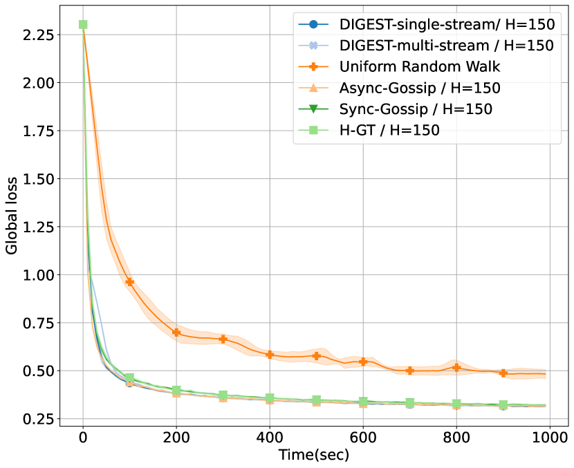
(a) 10-nodes / iid / balanced

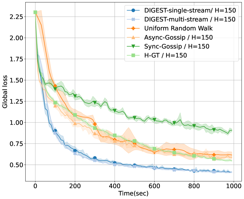
(b) 10-nodes / non-iid / unbalanced

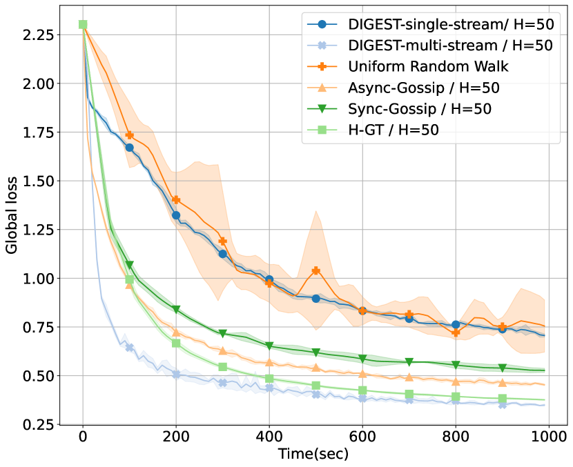
(c) 100-nodes / non-iid / unbalanced

Figure 4: Convergence results for MNIST dataset in terms of global loss over wall-clock time.

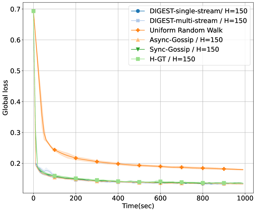
(a) 10-nodes / iid / balanced

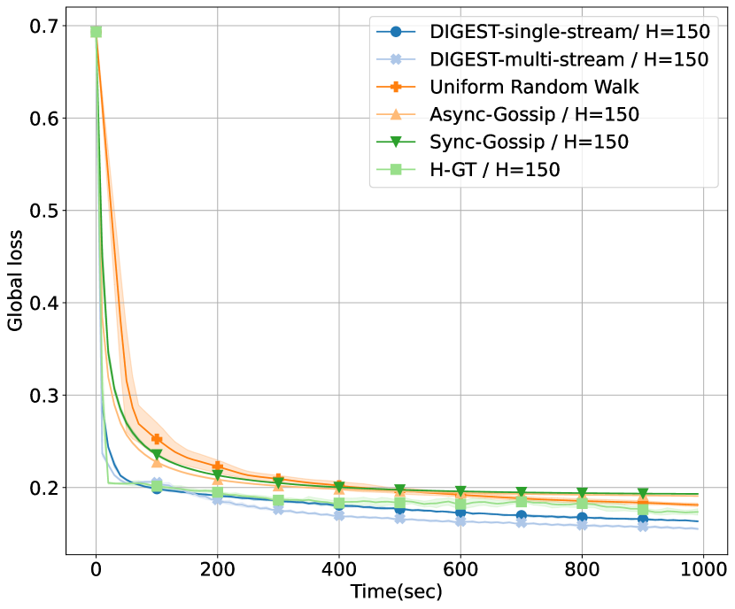
(b) 10-nodes / non-iid / unbalanced

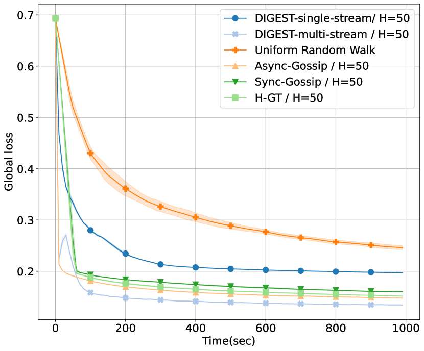
(c) 100-nodes / non-iid / unbalanced

Figure 5: Convergence results for w8a dataset in terms of global loss over wall-clock time.

We evaluate DIGEST as compared to baselines; (i) Uniform Random-Walk (URW) [24]: This is a random walk-based learning algorithm described in Fig. 1(c); (ii) Gradient tracking (GT) with local-SGD [45]: It is an algorithm that is developed to overcome data heterogeneity across nodes in a decentralized optimization problems; (iii) Async-Gossip [18] with local-SGD; (iv) (ii) Sync-Gossip [18] with local-SGD. Our codes are provided in [46].

We consider two network topologies; an Erdős–Rényi graph of $V=10$ and $V=100$ nodes with $0.3$ as the probability of connectivity. We assume that each iteration of Local SGD takes $0.1$ second. The communication delay between every two neighbors is assumed to have exponential distribution where its average is randomly chosen from $0$ to $5$ seconds.

We use two data distribution: (i) iid-balanced, and (ii) non-iid-unbalanced. In iid-balanced case, data is shuffled and equally divided and placed in nodes. Non-iid-unbalanced has two features: (i) Non-iid, which is realized by sorting data according to their labels, and distribute them in the sorted order. Thus, the data distributed over nodes will be non-iid; (ii) Unbalanced, which means that each node may have different amount of data. We use geometric series to realize unbalanced data across nodes. For example, if a node $u$ has $D_{u}=\delta$ data, the next nodes get $\delta\rho$, $\delta\rho^{2}$, etc. data, where $\rho$ is determined by taking into account the size of the total dataset $D$.

5.1 Logistic Regression

We examine the convergence performance of logistic regression, i.e., $f(\mathbf{x})$ $=$ $\frac{1}{D}$ $\sum_{i=1}^{D}\text{CrossEntropy}$ $\big{(}\text{softmax}(\mathbf{x}\mathbf{a_{i}}),b_{i}\big{)}+\frac{\lambda}{2}\|\mathbf{x}\|^{2}$, where $\mathbf{a_{i}}\in\mathbb{R}^{d}$, and $b_{i}$ are the feature and label of the data sample $i$. The regularization parameter is considered $\lambda=\frac{1}{D}$. We run the optimization using tuned constant learning rate for each algorithm. To grid-search the learning rate, we try the experiment with multiplying and dividing the learning rate by powers of two. This involves trying out both larger and smaller learning rates until we find the best result. We use datasets w8a [32] and MNIST [33]. The numerical experiments were run on Ubuntu $20.04$ using $36$ Intel Core i9-10980XE processors. For each experiment, we repeat $50$ times and present the error bars associated with the randomness of the optimization. In every figure, we include the average and standard deviation error bar.

Figs. 4 and 5 show the convergence behavior of our algorithms as well as the baselines for MNIST and w8a datasets in 10-nodes and 100-nodes topologies. URW generally underperforms as compared to other methods due to its approach of conducting only one local-SGD operation per iteration on a single node. As a consequence, it does not have a linear speed-up with increasing number of nodes. In certain situations involving non-iid data distribution, URW may exhibit better performance than some other methods as shown in Figs. 4(b), 4(c), 5(c), 5(c). This is because URW is not affected by non-iidness as it uniformly incorporates data from all nodes. DIGEST, Sync-Gossip, and Async-Gossip have similar performance in iid data distribution in Figs. 4(a), 5(a). On the other hand, we observe that Gossip based algorithms are suffering from slow convergence in non-iid setting as shown in Figs. 4(b), 4(c), 5(b), 5(c). We also observe that GT algorithms enhance the performance of gossip-based algorithms by incorporating a mechanism to overcome non-iidness. However, this algorithm demands twice the communication overhead compared to sync-Gossip, resulting in more communication overhead, which can degrade its convergence performance in terms of wall-clock time. In comparison, DIGEST have better convergence behavior thanks to its very design of spreading information uniformly in the network to handle non-iidness. It is evident that when the network is larger, one-stream DIGEST method is unable to cover the entire network as quickly as required, highlighting the need to utilize multi-stream DIGEST to overcome this limitation. This observation is supported in Figs. 4(c), 5(c), where all streams have the same $H_{m}=H,m\in\mathcal{M}$ in multi-stream DIGEST.

5.2 Deep Neural Network (DNN)

In this section, we use ResNet-$20$ [31] as the DNN model. The dataset is CIFAR-10 [34]. We have set the batch size to $36$ per node, and the learning rate is decayed by a constant factor after completing $50\%$ and $75\%$ of the training time. The initial value of the learning rate is separately tuned for each algorithm. We have set the momentum value to $0.9$ and the weight decay to $10^{-4}$. We observe that in the iid setting (Fig. 6(a)), all algorithms except URW perform similarly. However, in non-iid settings, where communication and model distribution across the network become crucial, DIGEST outperforms Gossip-based algorithms, Fig. 6(b).

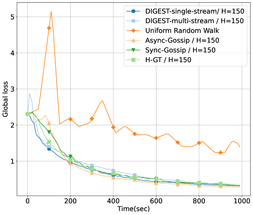
(a) 10-nodes / iid / balanced

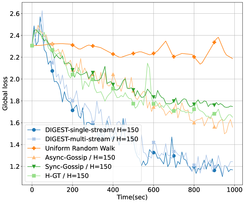
(b) 10-nodes / non-iid / unbalanced

Figure 6: Convergence results for CIFAR-10 dataset in terms of global loss over wall-clock time.

5.3 Speed-up

In this section, we evaluate the speed up performance of our DIGEST algorithms as well as the baseline; centralized parallel SGD. We consider the following cost function

$$f(x)=\begin{cases}(x-1)^{2}&\quad x\geq 1,\\ \frac{(x-1)^{2}}{2}&\quad x<1.\\ \end{cases}$$ (3)

We employ Local-SGD at node $v$ with gradients affected by a normal noise, i.e., $\nabla f_{i_{t}^{v}}(\mathbf{x}^{v}_{t})=\nabla f(\mathbf{x}^{v}_{t})+n_{t}^{v}$, where $n_{t}^{v}\sim\mathcal{N}(\zeta_{v},\sigma^{2})$, $\sum_{v=1}^{V}\zeta_{v}=0$. To create the speed-up curve, we divide the expected error of a single node SGD by the expected error of each method at the last iteration $T$ for different number of nodes. As in linear speed-up, error decreases linearly with the increasing number of workers, so we expect to see a straight line on the graph. The speed-up curve is illustrated in Fig. 7. The central parallel SGD averages all nodes‘ updates at every $H$ steps, and updates the model in all nodes. It is worth noting that the central parallel SGD with $H=1$ is the best speed-up that can be achieved in this scenario.

We set the learning rate to $0.001$, and $|\zeta_{v}|=5$ for $v\in\mathcal{V}$, $\sigma=5$, and $T=10^{4}$. Note that in iid setting with a less restrictive constraint on $H$, larger $H$ can still leads to linear speed-up when compared to non-iid setting. Moreover, it is seen that single stream DIGEST has linear speed-up to a certain limit; however, as the number of nodes increases and single-stream DIGEST cannot traverse the entire network fast enough, linear speed-up is not maintained. On the other hand, multi-stream DIGEST achieves linear speed up and achieves a very close performance to the best possible scenario, which is centralized parallel SGD with $H=1$.

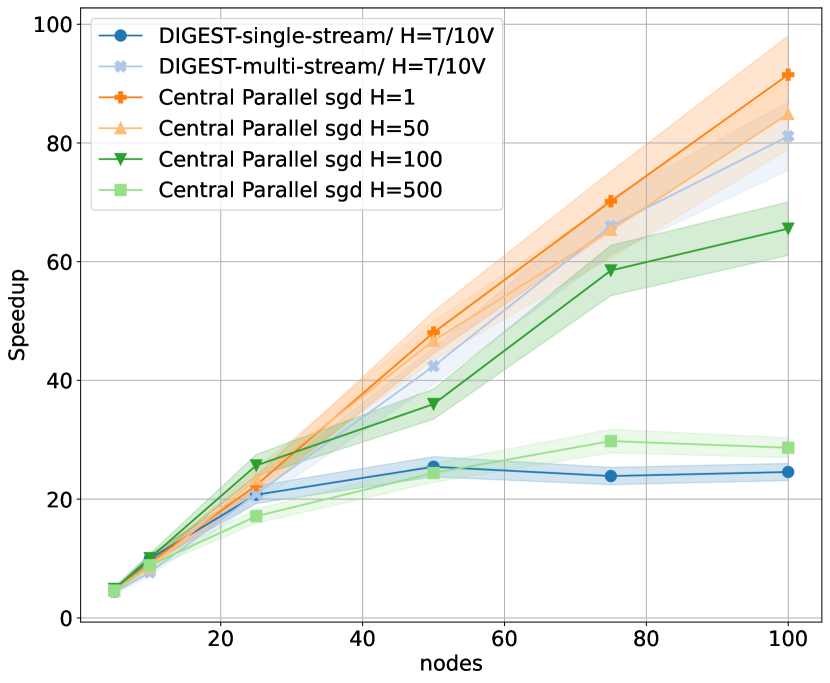
(a) iid / balanced

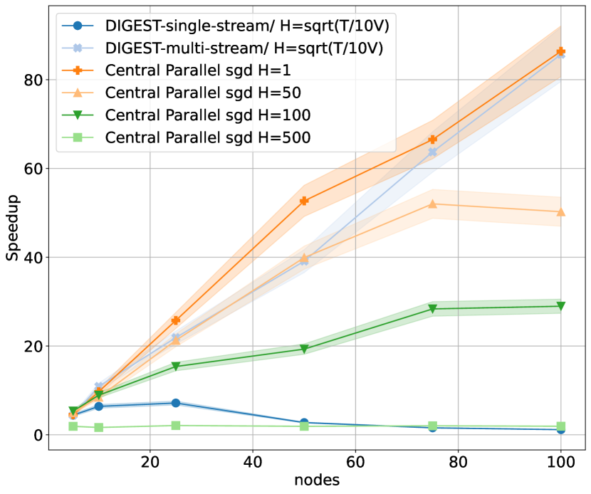
(b) non-iid / unbalanced

Figure 7: Speed-up curves for DIGEST.

6 Conclusion

We designed a fast and communication-efficient decentralized learning mechanism; DIGEST by particularly focusing on stochastic gradient descent (SGD). We designed single- and multi-stream DIGEST to exploit the convergence rate and communication overhead tradeoff. We analyzed the convergence of single- and multi-stream DIGEST, and proved that both algorithms approach to the optimal solution asymptotically for both iid and non-iid data. The simulation results confirms that the communication cost of DIGEST is low as compared to the baselines, and its convergence rate is better than or comparable to the baselines.

.1 Notation Table

$G=(\mathcal{V},\mathcal{E})$	Graph representing the network
$V$	Number of nodes
$\mathcal{D}$	The whole dataset in the network with size $D$
$\mathcal{D}_{v}$	Subset of $\mathcal{D}$ at node $v$ with size $D_{v}$
$f_{i}(\mathbf{x})$	Loss function of model $\mathbf{x}$ associated with the data sample $i$
$f(\mathbf{x})$	Global loss function of model $\mathbf{x}$
$f^{v}(\mathbf{x})$	Local loss function of model $\mathbf{x}$ at node $v$
$f^{*}$	$\min_{\mathbf{x}\in\mathbb{R}^{d}}f(\mathbf{x})$
$\mathbf{x}^{*}$	$\arg\min_{\mathbf{x}\in\mathbb{R}^{d}}f(\mathbf{x})$
$\mathbf{x}_{0}$	Initial model
$T$	Total number of iterations
$\eta_{t}$	Learning rate at iteration $t$
$l^{v}_{t}$	Completion time of local-SGD update started at $t$ in node $v$
${L}^{v}_{T}$	Set of $\{l^{v}_{t}\}_{0\leq t<T}$
$\mathbf{x}^{v}_{t}$	Local model in node $v$ at $t$
$s_{t}^{v}$	Binary variable that shows if node $v$ receives the global model at $t$ in single-stream DIGEST
$\mathcal{S}^{v}_{T}$	Set of $\{s^{v}_{t}\}_{0<t\leq T}$
$H$	Synchronization bound for single-stream DIGEST, i.e., $gap(\mathcal{S}^{v}_{T})\leq H$, $1\leq v\leq V$
$s_{t}^{v}[m]$	Binary variable that shows if node $v$ receives the global model at $t$ from stream $m$ in multi-stream DIGEST
$\mathcal{S}^{v}_{T}[m]$	$\{s^{v}_{t}[m]\}_{0<t\leq T}$
$H_{m}$	Synchronization bound of stream $m$ in multi-stream DIGEST, i.e., $gap(\mathcal{S}^{v}_{T}[m])\leq H_{m}$, $m\in\mathcal{M}_{v}$
$visited$	Set of nodes that are visited for the global model update in the most recent synchronization round for single-stream DIGEST
$visited[m]$	Set of nodes that are visited for the semi-global model update in the most recent synchronization round in stream $m$ for multi-stream DIGEST
$\tilde{\mathbf{x}}_{t}$	The global model received by node $v$ at $t$ in single-stream DIGEST
$\tilde{\mathbf{x}}_{t}[m]$	The global model received by node $v$ at $t$ from stream $m$ in multi-stream DIGEST
$pre\_node$	The node that node $v$ receives the global model from in single-stream DIGEST
$pre\_node[m]$	The node that node $v$ receives the semi-global model from in stream $m$ for multi-stream DIGEST
$p^{v}_{m}$	The node that node $v$ receives the global model from for the first time in the current synchronization round in stream $m$
$d^{G}_{uv}$	The distance between $u$ and $v$, the total delay of the links in the shortest path between $u$ and $v$
$R^{G}_{v}$	The greatest distance from $v$, i.e., $R^{G}_{v}=\max_{v}d^{G}_{uv}$
$r$	Root or the node with the minimum $R^{G}_{v}$, i.e., $r=\arg\min_{v}R^{G}_{v}$
$ST_{r}$	The shortest path tree rooted at r
$P^{r}_{v}$	Set of streams working over the path from $v$ to $r$ in $ST_{r}$
$M$	Number of streams in multi-stream DIGEST
$\mathcal{M}_{v}$	The set of streams passing node $v$
$\mathcal{V}_{m}$	The set of nodes in domain of stream $m$

.2 Proof of Theorem 4.1

Motivated by [27], a virtual sequence $\{\bar{\mathbf{x}}_{t}\}_{t\geq 0}$ is defined as follows.

$$\bar{\mathbf{x}}_{t}=\mathbf{x}_{0}-\sum_{v=1}^{V}\sum_{z=0}^{t-1}\frac{D_{v}}{D}\eta_{z}\nabla f_{i_{z}^{v}}(\mathbf{x}^{v}_{z}).$$ (4)

We do not need to calculate this sequence in the algorithm explicitly and it is only used for the sake of the analysis. We also define

$$\mathbf{g}_{t}=\sum_{v=1}^{V}\frac{D_{v}}{D}\nabla f_{i_{t}^{v}}(\mathbf{x}^{v}_{t}), \bar{\mathbf{g}}_{t}=\sum_{v=1}^{V}\frac{D_{v}}{D}\nabla f^{v}(\mathbf{x}^{v}_{t}),$$ (5)

where $f(\mathbf{x})$, $f^{v}(\mathbf{x})$ are global loss function and local loss function in node $v$, respectively.

Let us introduce $i_{t}=\{i_{t}^{1},...i_{t}^{V}\}$ to denote the data samples selected randomly during time slot $t$ in all nodes. Then, observe that $\bar{\mathbf{g}}_{t}=\operatorname{\mathbb{E}}_{i_{t}}\mathbf{g}_{t}$. $\mathbf{g}^{*}_{t}$ is the real true direction to go in opposite of in each step. We have $\bar{\mathbf{x}}_{t+1}=\bar{\mathbf{x}}_{t}-\eta_{t}\mathbf{g}_{t}$.

First, we illustrate how the virtual sequence, $\{\bar{\mathbf{x}}_{t}\}_{t\geq 0}$, approaches to the optimal in Lemma 1. Second, we depict in Lemma 2 that there is a little deviation from the virtual sequence in the actual iterates, $\mathbf{x}^{v}_{t}$. Finally, the convergence rate is proved.

Lemma .1.

If $f_{i_{t}^{v}}(\mathbf{x})$ is $L$-smooth, $f^{v}(\mathbf{x})$ is $\mu$-strongly convex, $\eta_{t}\leq\frac{1}{4L}$, and $\operatorname{\mathbb{E}}_{i^{v}_{t}}\|\nabla f_{i_{t}^{v}}(\mathbf{x}^{v}_{t})-\nabla f^{v}(\mathbf{x}^{v}_{t})\|^{2}\leq\sigma^{2}$ for $0\leq t\leq T-1$, $1\leq v\leq V$ then

$$\operatorname{\mathbb{E}}\|\bar{\mathbf{x}}_{t+1}-\mathbf{x}^{*}\|^{2}\leq(1-\mu\eta_{t})\operatorname{\mathbb{E}}\|\bar{\mathbf{x}}_{t}-\mathbf{x}^{*}\|^{2}+\eta_{t}^{2}\rho\sigma^{2}-\eta_{t}\operatorname{\mathbb{E}}(f(\bar{\mathbf{x}}_{t})-f(\mathbf{x}^{*}))+2L\eta_{t}\sum_{v=1}^{V}\frac{D_{v}}{D}\operatorname{\mathbb{E}}\|\mathbf{x}^{v}_{t}-\bar{\mathbf{x}}_{t}\|^{2}.$$ (6)

Proof.

We have

$$\|\bar{\mathbf{x}}_{t+1}-\mathbf{x}^{*}\|^{2}=\|\bar{\mathbf{x}}_{t}-\eta_{t}\mathbf{g}_{t}-\mathbf{x}^{*}\|^{2}=\|\bar{\mathbf{x}}_{t}-\mathbf{x}^{*}-\eta_{t}\bar{\mathbf{g}}_{t}+\eta_{t}\bar{\mathbf{g}}_{t}-\eta_{t}\mathbf{g}_{t}\|^{2}$$ (7)

$$=\|\bar{\mathbf{x}}_{t}-\mathbf{x}^{*}-\eta_{t}\bar{\mathbf{g}}_{t}\|^{2}+\eta^{2}_{t}\|\bar{\mathbf{g}}_{t}-\mathbf{g}_{t}\|^{2}+2\eta_{t}\langle\bar{\mathbf{x}}_{t}-\mathbf{x}^{*}-\eta_{t}\mathbf{g}^{*}_{t},\bar{\mathbf{g}}_{t}-\mathbf{g}_{t}\rangle$$ (8)

Then we apply expectation to get $\operatorname{\mathbb{E}}_{i_{0},...,i_{t}}\|\bar{\mathbf{x}}_{t+1}-\mathbf{x}^{*}\|^{2}$. Based on the law of total expectation, for every two random variables $\alpha$, $\beta$ and a function $y$, $\operatorname{\mathbb{E}}_{\alpha}y(\alpha)=\operatorname{\mathbb{E}}_{\beta}\operatorname{\mathbb{E}}_{\alpha}[y(\alpha)|\beta]$. Considering $\alpha=i_{0},...,i_{t}$ and $\beta=i_{0},...,i_{t-1}$, we get that

$$\operatorname{\mathbb{E}}_{i_{0},...,i_{t}}\langle\bar{\mathbf{x}}_{t}-\mathbf{x}^{*}-\eta_{t}\bar{\mathbf{g}}_{t},\bar{\mathbf{g}}_{t}-\mathbf{g}_{t}\rangle =\operatorname{\mathbb{E}}_{i_{0},...,i_{t-1}}\operatorname{\mathbb{E}}_{i_{0},...,i_{t}}[\langle\bar{\mathbf{x}}_{t}-\mathbf{x}^{*}-\eta_{t}\bar{\mathbf{g}}_{t},\bar{\mathbf{g}}_{t}-\mathbf{g}_{t}\rangle|i_{0},...,i_{t-1}]$$ (9)

$$=\operatorname{\mathbb{E}}_{i_{0},...,i_{t-1}}\langle\bar{\mathbf{x}}_{t}-\mathbf{x}^{*}-\eta_{t}\bar{\mathbf{g}}_{t},\bar{\mathbf{g}}_{t}-\operatorname{\mathbb{E}}_{i_{t}}\mathbf{g}_{t}\rangle$$ (10)

$$=\operatorname{\mathbb{E}}_{i_{0},...,i_{t}}\langle\bar{\mathbf{x}}_{t}-\mathbf{x}^{*}-\eta_{t}\bar{\mathbf{g}}_{t},\bar{\mathbf{g}}_{t}-\operatorname{\mathbb{E}}_{i_{t}}\mathbf{g}_{t}\rangle$$ (11)

$$=\operatorname{\mathbb{E}}_{i_{0},...,i_{t}}\langle\bar{\mathbf{x}}_{t}-\mathbf{x}^{*}-\eta_{t}\bar{\mathbf{g}}_{t},\bar{\mathbf{g}}_{t}-\bar{\mathbf{g}}_{t}\rangle$$ (12)

$$=0$$ (13)

In (10), we used the fact that once we know $i_{0},...,i_{t-1}$, the value of $\mathbf{x}^{v}_{t}$, $1\leq v\leq V$, and therefore $\bar{\mathbf{x}}_{t}$ and $\bar{\mathbf{g}}_{t}$ are not random any more. From now on, we drop the subscript $i_{0},...,i_{t}$ for the ease of notation. Thus,

$$\operatorname{\mathbb{E}}\|\bar{\mathbf{x}}_{t+1}-\mathbf{x}^{*}\|^{2}\leq \operatorname{\mathbb{E}}\|\bar{\mathbf{x}}_{t}-\mathbf{x}^{*}-\eta_{t}\bar{\mathbf{g}}_{t}\|^{2}+\eta^{2}_{t}\operatorname{\mathbb{E}}\|\bar{\mathbf{g}}_{t}-\mathbf{g}_{t}\|^{2}$$ (14)

We obtain

$$\|\bar{\mathbf{x}}_{t}-\mathbf{x}^{*}-\eta_{t}\bar{\mathbf{g}}_{t}\|^{2} =\|\bar{\mathbf{x}}_{t}-\mathbf{x}^{*}\|^{2}+\eta_{t}^{2}\|\bar{\mathbf{g}}_{t}\|^{2}-2\eta_{t}\langle\bar{\mathbf{x}}_{t}-\mathbf{x}^{*},\bar{\mathbf{g}}_{t}\rangle$$ (15)

$$=\|\bar{\mathbf{x}}_{t}-\mathbf{x}^{*}\|^{2}+\eta_{t}^{2}\|\bar{\mathbf{g}}_{t}\|^{2}-2\eta_{t}\sum_{v=1}^{V}\frac{D_{v}}{D}\langle\bar{\mathbf{x}}_{t}-\mathbf{x}^{v}_{t}+\mathbf{x}^{v}_{t}-\mathbf{x}^{*},\nabla f^{v}(\mathbf{x}^{v}_{t})\rangle$$ (16)

$$=\|\bar{\mathbf{x}}_{t}-\mathbf{x}^{*}\|^{2}+\eta^{2}\|\sum_{v=1}^{V}\frac{D_{v}}{D}\nabla f^{v}(\mathbf{x}^{v}_{t})\|^{2}-2\eta_{t}\sum_{v=1}^{V}\frac{D_{v}}{D}\langle\mathbf{x}^{v}_{t}-\mathbf{x}^{*},\nabla f^{v}(\mathbf{x}^{v}_{t})\rangle$$ (17)

$$\mathllap{-2\eta\sum_{v=1}^{V}\frac{D_{v}}{D}\langle\bar{\mathbf{x}}_{t}-\mathbf{x}^{v}_{t},\nabla f^{v}(\mathbf{x}^{v}_{t})\rangle}$$

We obtain

$$\|\sum_{v=1}^{V}\frac{D_{v}}{D}\nabla f^{v}(\mathbf{x}^{v}_{t})\|^{2} =\|\sum_{v=1}^{V}\frac{D_{v}}{D}(\nabla f^{v}(\mathbf{x}^{v}_{t})-\nabla f^{v}(\bar{\mathbf{x}}_{t})+\nabla f^{v}(\bar{\mathbf{x}}_{t})-\nabla f^{v}(\mathbf{x}^{*}))\|^{2}$$ (18)

$$\leq 2\|\sum_{v=1}^{V}\frac{D_{v}}{D}(\nabla f^{v}(\mathbf{x}^{v}_{t})-\nabla f^{v}(\bar{\mathbf{x}}_{t}))\|^{2}+2\|\sum_{v=1}^{V}\frac{D_{v}}{D}(\nabla f^{v}(\bar{\mathbf{x}}_{t})-\nabla f^{v}(\mathbf{x}^{*}))\|^{2}$$ (19)

$$\leq 2\|\sum_{v=1}^{V}\frac{D_{v}}{D}(\nabla f^{v}(\mathbf{x}^{v}_{t})-\nabla f^{v}(\bar{\mathbf{x}}_{t}))\|^{2}+2\|\nabla f(\bar{\mathbf{x}}_{t})-\nabla f(\mathbf{x}^{*})\|^{2}$$ (20)

$$\leq 2\sum_{v=1}^{V}\frac{D_{v}}{D}\|(\nabla f^{v}(\mathbf{x}^{v}_{t})-\nabla f^{v}(\bar{\mathbf{x}}_{t}))\|^{2}+2\|(\nabla f(\bar{\mathbf{x}}_{t})-\nabla f(\mathbf{x}^{*}))\|^{2}$$ (21)

$$\leq 2L^{2}\sum_{v=1}^{V}\frac{D_{v}}{D}\|\mathbf{x}^{v}_{t}-\bar{\mathbf{x}}_{t}\|^{2}+4L(f(\bar{\mathbf{x}}_{t})-f(\mathbf{x}^{*}))$$ (22)

where (19) is based on the following inequality.

$$\|\sum_{i=1}^{n}a_{i}\|^{2}\leq n\sum_{i=1}^{n}\|a_{i}\|^{2}.$$ (23)

In (20) we have used the fact that $\sum_{v=1}^{V}\frac{D_{v}}{D}f^{v}(\mathbf{x})=f(\mathbf{x})$. (21), and (22) are due to the convexity of $\|.\|^{2}$ and L-smoothness, respectively. Note that by $L$-smoothness we have

$$\|\nabla f(\mathbf{x})-\nabla f(\mathbf{x}^{*})\|^{2}\leq 2L(f(\mathbf{x})-f^{*}).$$ (24)

$\mu$-strong convexity provides us with

$$-\langle\mathbf{x}^{v}_{t}-\mathbf{x}^{*},\nabla f^{v}(\mathbf{x}^{v}_{t})\rangle\leq-(f^{v}(\mathbf{x}^{v}_{t})-f^{v}(\mathbf{x}^{*}))-\frac{\mu}{2}\|\mathbf{x}^{v}_{t}-\mathbf{x}^{*}\|^{2}.$$ (25)

Using $L$-smoothness to bound the last term in (17), we have

$$-\langle\bar{\mathbf{x}}_{t}-\mathbf{x}^{v}_{t},\nabla f^{v}(\mathbf{x}^{v}_{t})\rangle \leq f(\mathbf{x}^{v}_{t})-f(\bar{\mathbf{x}}_{t})+\frac{L}{2}\|\mathbf{x}^{v}_{t}-\bar{\mathbf{x}}_{t}\|^{2}$$ (26)

We obtain the following result by applying (22), (25), and (26) to (17):

$$\|\bar{\mathbf{x}}_{t}-\eta_{t}\mathbf{g}^{*}_{t}-\mathbf{x}^{*}\|^{2}\leq\|\bar{\mathbf{x}}_{t}-\mathbf{x}^{*}\|^{2}+2L^{2}\eta_{t}^{2}\sum_{v=1}^{V}\frac{D_{v}}{D}\|\mathbf{x}^{v}_{t}-\bar{\mathbf{x}}_{t}\|^{2}+4L\eta_{t}^{2}(f(\bar{\mathbf{x}}_{t})-f(\mathbf{x}^{*}))$$ (27)

$$\mathllap{+2\eta_{t}\sum_{v=1}^{V}\frac{D_{v}}{D}\big{(}-(f^{v}(\mathbf{x}^{v}_{t})-f^{v}(\mathbf{x}^{*}))-\frac{\mu}{2}\|\mathbf{x}^{v}_{t}-\mathbf{x}^{*}\|^{2}+f(\mathbf{x}^{v}_{t})-f(\bar{\mathbf{x}}_{t})+\frac{L}{2}\|\mathbf{x}^{v}_{t}-\bar{\mathbf{x}}_{t}\|^{2}\big{)}}.$$

This can be rewritten as

$$\|\bar{\mathbf{x}}_{t}-\eta_{t}\mathbf{g}^{*}_{t}-\mathbf{x}^{*}\|^{2}\leq\|\bar{\mathbf{x}}_{t}-\mathbf{x}^{*}\|^{2}+2\eta(2L\eta_{t}-1)(f(\bar{\mathbf{x}}_{t})-f(\mathbf{x}^{*}))+L\eta_{t}(1+2L\eta_{t})\sum_{v=1}^{V}\frac{D_{v}}{D}\|\mathbf{x}^{v}_{t}-\bar{\mathbf{x}}_{t}\|^{2}.$$ (28)

$$\mathllap{-\mu\eta\|\mathbf{x}^{v}_{t}-\mathbf{x}^{*}\|^{2}}$$

Using concavity of $\beta\|\mathbf{x}^{v}_{t}-\mathbf{x}^{*}\|^{2}$ for $\beta\leq 0$, we get

$$-\mu\|\mathbf{x}^{v}_{t}-\mathbf{x}^{*}\|^{2}\leq-\mu\|\bar{\mathbf{x}}_{t}-\mathbf{x}^{*}\|^{2},$$ (29)

so we get

$$\|\bar{\mathbf{x}}_{t}-\eta_{t}\mathbf{g}^{*}_{t}-\mathbf{x}^{*}\|^{2}\leq(1-\mu\eta_{t})\|\bar{\mathbf{x}}_{t}-\mathbf{x}^{*}\|^{2}+2\eta(2L\eta_{t}-1)(f(\bar{\mathbf{x}}_{t})-f(\mathbf{x}^{*}))+L\eta_{t}(1+2L\eta_{t})\sum_{v=1}^{V}\frac{D_{v}}{D}\|\mathbf{x}^{v}_{t}-\bar{\mathbf{x}}_{t}\|^{2}.$$ (30)

we have $(2\eta_{t}L-1)\leq-\frac{1}{2}$, $(2\eta_{t}L+1)\leq 2$ as we assumed $\eta_{t}\leq\frac{1}{4L}$. So we obtain

$$\|\bar{\mathbf{x}}_{t}-\eta_{t}\mathbf{g}^{*}_{t}-\mathbf{x}^{*}\|^{2}\leq(1-\mu\eta_{t})\|\bar{\mathbf{x}}_{t}-\mathbf{x}^{*}\|^{2}-\eta(f(\bar{\mathbf{x}}_{t})-f(\mathbf{x}^{*}))+2L\eta_{t}\sum_{v=1}^{V}\frac{D_{v}}{D}\|\mathbf{x}^{v}_{t}-\bar{\mathbf{x}}_{t}\|^{2}.$$ (31)

We have by definition that

$$\operatorname{\mathbb{E}}\|\mathbf{g}_{t}-\bar{\mathbf{g}}_{t}\|^{2} =\operatorname{\mathbb{E}}\|\sum_{v=1}^{V}\frac{D_{v}}{D}(\nabla f_{i_{t}^{v}}(\mathbf{x}^{v}_{t})-\nabla f^{v}(\mathbf{x}^{v}_{t}))\|^{2}$$ (32)

$$=\sum_{v=1}^{V}(\frac{D_{v}}{D})^{2}\operatorname{\mathbb{E}}\|(\nabla f_{i_{t}^{v}}(\mathbf{x}^{v}_{t})-\nabla f^{v}(\mathbf{x}^{v}_{t})\|^{2}$$ (33)

$$=\sigma^{2}\sum_{v=1}^{V}(\frac{D_{v}}{D})^{2}$$ (34)

$$=\rho\sigma^{2},$$ (35)

where (33) is based on the fact that variance of the sum of independent random variables equals sum of their variances.

Taking expectation of (31) and applying it with (35) into (14) provides

$$\operatorname{\mathbb{E}}\|\bar{\mathbf{x}}_{t+1}-\mathbf{x}^{*}\|^{2}\leq(1-\mu\eta_{t})\operatorname{\mathbb{E}}\|\bar{\mathbf{x}}_{t}-\mathbf{x}^{*}\|^{2}+\eta_{t}^{2}\rho\sigma^{2}-\eta_{t}\operatorname{\mathbb{E}}(f(\bar{\mathbf{x}}_{t})-f(\mathbf{x}^{*}))+2L\eta_{t}\sum_{v=1}^{V}\frac{D_{v}}{D}\operatorname{\mathbb{E}}\|\mathbf{x}^{v}_{t}-\bar{\mathbf{x}}_{t}\|^{2}.$$ (36)

∎

Lemma .2.

If $f^{v}(\mathbf{x})$ is $L$-smooth , $\eta_{t}\leq\frac{1}{4L}$, and $\operatorname{\mathbb{E}}_{i^{v}_{t}}\|\nabla f_{i_{t}^{v}}(\mathbf{x}^{v}_{t})-\nabla f^{v}(\mathbf{x}^{v}_{t})\|^{2}\leq\sigma^{2}$ for $0\leq t\leq T-1$, $1\leq v\leq V$ then

$$\operatorname{\mathbb{E}}f(\bar{\mathbf{x}}_{t+1})\leq\operatorname{\mathbb{E}}f(\bar{\mathbf{x}}_{t})+\frac{\eta_{t}^{2}L\rho\sigma^{2}}{2}-\frac{\eta_{t}}{4}\operatorname{\mathbb{E}}\|\nabla f(\bar{\mathbf{x}}_{t})\|^{2}+L^{2}\eta_{t}\sum_{v=1}^{V}\frac{D_{v}}{D}\operatorname{\mathbb{E}}\|\mathbf{x}^{v}_{t}-\bar{\mathbf{x}}_{t}\|^{2}.$$ (37)

Proof.

Based on the defenition of $\bar{\mathbf{x}}_{t}$ and L-smoothness of $f^{v}(\mathbf{x})$ we have

$$f(\bar{\mathbf{x}}_{t+1}) =f(\bar{\mathbf{x}}_{t}-\eta_{t}\mathbf{g}_{t})$$ (38)

$$\leq f(\bar{\mathbf{x}}_{t})+\eta_{t}\langle\nabla f(\bar{\mathbf{x}}_{t}),-\mathbf{g}_{t}\rangle+\frac{\eta_{t}^{2}L}{2}\|\mathbf{g}_{t}\|^{2}$$ (39)

Lets take Expectation of the second term on the right-hand side of (39)

$$\eta_{t}\operatorname{\mathbb{E}}\langle\nabla f(\bar{\mathbf{x}}_{t}),-\mathbf{g}_{t}\rangle =\eta_{t}\operatorname{\mathbb{E}}\langle\nabla f(\bar{\mathbf{x}}_{t}),\nabla f(\bar{\mathbf{x}}_{t})-\nabla f(\bar{\mathbf{x}}_{t})-\bar{\mathbf{g}}_{t}\rangle$$ (40)

$$=-\eta_{t}\operatorname{\mathbb{E}}\|\nabla f(\bar{\mathbf{x}}_{t})\|^{2}+\eta_{t}\operatorname{\mathbb{E}}\langle\nabla f(\bar{\mathbf{x}}_{t}),\nabla f(\bar{\mathbf{x}}_{t})-\bar{\mathbf{g}}_{t}\rangle$$ (41)

$$\leq-\eta_{t}\operatorname{\mathbb{E}}\|\nabla f(\bar{\mathbf{x}}_{t})\|^{2}+\frac{\eta_{t}}{2}\operatorname{\mathbb{E}}\|\nabla f(\bar{\mathbf{x}}_{t})\|^{2}+\frac{\eta_{t}}{2}\operatorname{\mathbb{E}}\|\nabla f(\bar{\mathbf{x}}_{t})-\bar{\mathbf{g}}_{t}\|^{2}$$ (42)

$$\leq-\frac{\eta_{t}}{2}\operatorname{\mathbb{E}}\|\nabla f(\bar{\mathbf{x}}_{t})\|^{2}+\frac{\eta_{t}}{2}\operatorname{\mathbb{E}}\|\sum_{v=1}^{V}\frac{D_{v}}{D}(\nabla f^{v}(\bar{\mathbf{x}}_{t})-\nabla f^{v}(\mathbf{x}^{v}_{t}))\|^{2}$$ (43)

$$\leq-\frac{\eta_{t}}{2}\operatorname{\mathbb{E}}\|\nabla f(\bar{\mathbf{x}}_{t})\|^{2}+\frac{\eta_{t}}{2}\sum_{v=1}^{V}\frac{D_{v}}{D}\operatorname{\mathbb{E}}\|\nabla f^{v}(\bar{\mathbf{x}}_{t})-\nabla f^{v}(\mathbf{x}^{v}_{t})\|^{2}$$ (44)

$$\leq-\frac{\eta_{t}}{2}\operatorname{\mathbb{E}}\|\nabla f(\bar{\mathbf{x}}_{t})\|^{2}+\frac{\eta_{t}L^{2}}{2}\sum_{v=1}^{V}\frac{D_{v}}{D}\operatorname{\mathbb{E}}\|\bar{\mathbf{x}}_{t}-\mathbf{x}^{v}_{t}\|^{2}.$$ (45)

(42) is based on the fact that for any $\lambda>0$,

$$2\langle a,b\rangle\leq\lambda\|a\|^{2}+\frac{1}{\lambda}\|b\|^{2}.$$ (46)

(44) is based on the convexity of $\|.\|^{2}$ and (45) is due to $L$-smoothness.

Lets take Expectation of the last term on the right-hand side of (39)

$$\frac{\eta_{t}^{2}L}{2}\operatorname{\mathbb{E}}\|\mathbf{g}_{t}\|^{2} \leq\frac{\eta_{t}^{2}L}{2}\operatorname{\mathbb{E}}\|\mathbf{g}_{t}-\bar{\mathbf{g}}_{t}\|^{2}+\frac{\eta_{t}^{2}L}{2}\operatorname{\mathbb{E}}\|\bar{\mathbf{g}}_{t}\|^{2}$$ (47)

$$\leq\frac{\eta_{t}^{2}L}{2}\rho\sigma^{2}+\eta_{t}^{2}L^{3}\sum_{v=1}^{V}\frac{D_{v}}{D}\operatorname{\mathbb{E}}\|\mathbf{x}^{v}_{t}-\bar{\mathbf{x}}_{t}\|^{2}+\eta_{t}^{2}L\operatorname{\mathbb{E}}\|\nabla f(\bar{\mathbf{x}}_{t})\|^{2},$$ (48)

where (48) is based on (22),and (35). Putting everything together, we obtain

$$\operatorname{\mathbb{E}}f(\bar{\mathbf{x}}_{t+1})\leq\operatorname{\mathbb{E}}f(\bar{\mathbf{x}}_{t})+\frac{\eta_{t}^{2}L\rho\sigma^{2}}{2}+\eta_{t}(\eta_{t}L-\frac{1}{2})\operatorname{\mathbb{E}}\|\nabla f(\bar{\mathbf{x}}_{t})\|^{2}+L^{2}\eta_{t}(\eta_{t}L+\frac{1}{2})\sum_{v=1}^{V}\frac{D_{v}}{D}\operatorname{\mathbb{E}}\|\mathbf{x}^{v}_{t}-\bar{\mathbf{x}}_{t}\|^{2}.$$ (49)

considering $\eta_{t}\leq\frac{1}{4L}$ we obtain

$$\operatorname{\mathbb{E}}f(\bar{\mathbf{x}}_{t+1})\leq\operatorname{\mathbb{E}}f(\bar{\mathbf{x}}_{t})+\frac{\eta_{t}^{2}L\rho\sigma^{2}}{2}-\frac{\eta_{t}}{4}\operatorname{\mathbb{E}}\|\nabla f(\bar{\mathbf{x}}_{t})\|^{2}+L^{2}\eta_{t}\sum_{v=1}^{V}\frac{D_{v}}{D}\operatorname{\mathbb{E}}\|\mathbf{x}^{v}_{t}-\bar{\mathbf{x}}_{t}\|^{2}.$$ (50)

∎

Observe that Lemmas .1, .2 hold regardless of how to synchronize the nodes, i.e., hold for both single and multi-stream DIGEST.

Before going to the next lemma, we define $\tau$-slow sequences [47], $\{a_{t}\}_{t\geq 0}$ of positive values is $\tau$-slow decreasing for parameter $\tau\geq 1$ if

$$a_{t}\geq a_{t+1},\qquad a_{t}\leq a_{t+1}(1+\frac{1}{2\tau}),\qquad t\geq 0.$$ (51)

The sequence $\{a_{t}\}_{t\geq 0}$ is $\tau$-slow increasing if $\{a_{t}^{-1}\}_{t\geq 0}$ is $\tau$-slow decreasing.

Lemma .3 (Bounding deviation).

If $\max\{l^{v}_{t}-t\}\leq E$, $\operatorname{\mathbb{E}}_{i^{v}_{t}}\|\nabla f_{i_{t}^{v}}(\mathbf{x}^{v}_{t})-\nabla f^{v}(\mathbf{x}^{v}_{t})\|^{2}\leq\sigma^{2}$ ,$\|\nabla f^{v}(\mathbf{x}^{v}_{t})-\nabla f^{v}(\mathbf{x}^{v}_{t})\|^{2}\leq\zeta^{2}$, $\eta_{t}=\eta\leq\frac{1}{30L(H^{\prime}+E)}$, and $\omega_{t}$ is $(H^{\prime}+E)$-slow increasing for $0\leq t\leq T-1$, $1\leq v\leq V$, and for (i) single-stream DIGEST $gap(\mathcal{S}^{v}_{T})\leq H$, $1\leq v\leq V$, (ii) multi-stream DIGEST, $gap(\mathcal{S}^{v}_{T}[m])\leq H_{m}$ for $v$ that $m\in\mathcal{M}_{v}$,

$$\sum_{t=0}^{T-1}\omega_{t}\sum_{v=1}^{V}\frac{D_{v}}{D}\operatorname{\mathbb{E}}\|\bar{\mathbf{x}}_{t}-\mathbf{x}^{v}_{t}\|^{2}\leq\frac{1}{8L^{2}}\sum_{t=0}^{T-1}\omega_{t}\operatorname{\mathbb{E}}\|\nabla f(\bar{\mathbf{x}}_{t})\|^{2}+90\eta^{2}(H^{\prime}+E)\big{(}\zeta^{2}(H^{\prime}+E)+\sigma^{2}\big{)}\sum_{t=0}^{T-1}\omega_{t}.$$ (52)

where in single-stream $H^{\prime}=H$ and in multi-stream DIGEST $H^{\prime}=\max_{u}\sum_{m\in p_{u}^{v}}H_{m}$.

Proof.

First we focus on the single stream case, $\tau^{v}_{t}$ denotes the last time slot up to $t$, when node $v$’s model was updated with the synchronization stream, i.e., $\tau^{v}_{t}=\max\{t^{\prime}\mid t^{\prime}\leq t,s_{t^{\prime}}^{v}=1\}$. Lets use (23) to decompose the the deviation term as depicted in the following:

$$\|\bar{\mathbf{x}}_{t}-\mathbf{x}^{v}_{t}\|^{2}\leq 2(\|\mathbf{x}^{v}_{t}-\tilde{\mathbf{x}}_{\tau_{t}^{v}}\|^{2}+\|\bar{\mathbf{x}}_{t}-\tilde{\mathbf{x}}_{\tau_{t}^{v}}\|^{2}).$$ (53)

For the first term we can obtain

$$\operatorname{\mathbb{E}}\|\mathbf{x}^{v}_{t}-\tilde{\mathbf{x}}_{\tau_{t}^{v}}\|^{2} =\operatorname{\mathbb{E}}\|\mathbf{x}^{v}_{t}-\mathbf{x}^{v}_{\tau_{t}^{v}}\|^{2}$$ (54)

$$=\operatorname{\mathbb{E}}\|\sum_{t^{\prime}=\tau_{t}^{v}}^{t-1}\sum_{z\in u^{v}_{t^{\prime}}}\eta_{z}\nabla f_{i_{z}^{v}}(\mathbf{x}^{v}_{z})\|^{2}$$ (55)

$$=\operatorname{\mathbb{E}}\|\sum_{z\in\cup_{t^{\prime}=\tau_{t}^{v}}^{t-1}u^{v}_{t^{\prime}}}\eta_{z}\nabla f_{i_{z}^{v}}(\mathbf{x}^{v}_{z})\|^{2}.$$ (56)

And we have

$$\nabla f_{i_{z}^{v}}(\mathbf{x}^{v}_{z}) =\big{(}\nabla f_{i_{z}^{v}}(\mathbf{x}^{v}_{z})-\nabla f^{v}(\mathbf{x}^{v}_{z})\big{)}+\nabla f^{v}(\mathbf{x}^{v}_{z})$$ (57)

$$=\big{(}\nabla f_{i_{z}^{v}}(\mathbf{x}^{v}_{z})-\nabla f^{v}(\mathbf{x}^{v}_{z})\big{)}+\big{(}\nabla f^{v}(\mathbf{x}^{v}_{z})-\nabla f^{v}(\bar{\mathbf{x}}_{z})\big{)}+\nabla f^{v}(\bar{\mathbf{x}}_{z})$$ (58)

$$=\big{(}\nabla f_{i_{z}^{v}}(\mathbf{x}^{v}_{z})-\nabla f^{v}(\mathbf{x}^{v}_{z})\big{)}+\big{(}\nabla f^{v}(\mathbf{x}^{v}_{z})-\nabla f^{v}(\bar{\mathbf{x}}_{z})\big{)}+\big{(}\nabla f^{v}(\bar{\mathbf{x}}_{z})-\nabla f(\bar{\mathbf{x}}_{z})\big{)}+\nabla f(\bar{\mathbf{x}}_{z}),$$ (59)

so we can rewrite the right-hand side of (56) as

$$\operatorname{\mathbb{E}}\|\sum_{\mathcal{U}^{v}_{t}}\eta_{z}\nabla f_{i_{z}^{v}}(\mathbf{x}^{v}_{z})\|^{2} =4\operatorname{\mathbb{E}}\Big{(}\|\sum_{z\in\mathcal{U}^{v}_{t}}\eta_{z}\nabla f(\bar{\mathbf{x}}_{z})\|^{2}+\|\sum_{z\in\mathcal{U}^{v}_{t}}\eta_{z}\big{(}\nabla f^{v}(\mathbf{x}^{v}_{z})-\nabla f^{v}(\bar{\mathbf{x}}_{z})\big{)}\|^{2}$$ (60)

$$\mathllap{+\|\sum_{z\in\mathcal{U}^{v}_{t}}\eta_{z}\big{(}\nabla f^{v}(\bar{\mathbf{x}}_{z})-\nabla f(\bar{\mathbf{x}}_{z})\big{)}\|^{2}+\|\sum_{z\in\mathcal{U}^{v}_{t}}\eta_{z}\big{(}\nabla f_{i_{z}^{v}}(\mathbf{x}^{v}_{z})-\nabla f^{v}(\mathbf{x}^{v}_{z})\big{)}\|^{2}\Big{)}},$$

where $\mathcal{U}^{v}_{t}=\cup_{t^{\prime}=\tau_{t}^{v}}^{t-1}u^{v}_{t^{\prime}}$. Now we sum over $v$, multiply by $\omega_{t}$, and sum over $t$ and bound every term in (60) as follows. Considering that we have $|\mathcal{U}^{v}_{t}|\leq H+E$ we obtain

$$\sum_{t=0}^{T-1}\omega_{t}\sum_{v=1}^{V}\frac{D_{v}}{D}\|\sum_{z\in\mathcal{U}^{v}_{t}}\eta_{z}\nabla f(\bar{\mathbf{x}}_{z})\|^{2} \leq\sum_{t=0}^{T-1}\omega_{t}\sum_{v=1}^{V}\frac{D_{v}}{D}|\mathcal{U}^{v}_{t}|\sum_{z\in\mathcal{U}^{v}_{t}}\|\eta_{z}\nabla f(\bar{\mathbf{x}}_{z})\|^{2}$$ (61)

$$\leq(H+E)\sum_{t=0}^{T-1}\omega_{t}\sum_{v=1}^{V}\frac{D_{v}}{D}\sum_{z\in\mathcal{U}^{v}_{t}}\eta_{z}^{2}\|\nabla f(\bar{\mathbf{x}}_{z})\|^{2}$$ (62)

$$\leq 2(H+E)\sum_{v=1}^{V}\frac{D_{v}}{D}\ \sum_{t=0}^{T-1}\sum_{z\in\mathcal{U}^{v}_{t}}\omega_{z}\eta_{z}^{2}\|\nabla f(\bar{\mathbf{x}}_{z})\|^{2}$$ (63)

$$\leq 2(H+E)^{2}\sum_{v=1}^{V}\frac{D_{v}}{D}\ \sum_{t=0}^{T-1}\omega_{t}\eta_{t}^{2}\|\nabla f(\bar{\mathbf{x}}_{t})\|^{2}$$ (64)

$$\leq 2(H+E)^{2}\sum_{t=0}^{T-1}\omega_{t}\eta_{t}^{2}\|\nabla f(\bar{\mathbf{x}}_{t})\|^{2},$$ (65)

where (63) is due to the fact that $\omega_{t}\leq\omega_{t-z}(1+\frac{1}{2(H+E)})^{z}\leq\omega_{t-z}(1+\frac{1}{2(H+E)})^{H+E}\leq\omega_{t-z}\exp{(\frac{1}{2})}\leq 2\omega_{t-z}$ for $0\leq z\leq H+E$, i.e., $\omega_{t}$ is $(H+E)$-slow increasing. The second term in the right-hand side of (60) is bounded as

$$\sum_{t=0}^{T-1}\omega_{t}\sum_{v=1}^{V}\frac{D_{v}}{D}\|\sum_{z\in\mathcal{U}^{v}_{t}}\eta_{z} \big{(}\nabla f^{v}(\mathbf{x}^{v}_{z})-\nabla f^{v}(\bar{\mathbf{x}}_{z})\big{)}\|^{2}$$ (66)

$$\leq\sum_{t=0}^{T-1}\omega_{t}\sum_{v=1}^{V}\frac{D_{v}}{D}|\mathcal{U}^{v}_{t}|\sum_{z\in\mathcal{U}^{v}_{t}}\|\eta_{z}\big{(}\nabla f^{v}(\mathbf{x}^{v}_{z})-\nabla f^{v}(\bar{\mathbf{x}}_{z})\big{)}\|^{2}$$ (67)

$$\leq(H+E)\sum_{t=0}^{T-1}\omega_{t}\sum_{v=1}^{V}\frac{D_{v}}{D}\sum_{z\in\mathcal{U}^{v}_{t}}\eta_{z}^{2}\|\big{(}\nabla f^{v}(\mathbf{x}^{v}_{z})-\nabla f^{v}(\bar{\mathbf{x}}_{z})\big{)}\|^{2}$$ (68)

$$\leq 2(H+E)\sum_{v=1}^{V}\frac{D_{v}}{D}\ \sum_{t=0}^{T-1}\sum_{z\in\mathcal{U}^{v}_{t}}\omega_{z}\eta_{z}^{2}\|\big{(}\nabla f^{v}(\mathbf{x}^{v}_{z})-\nabla f^{v}(\bar{\mathbf{x}}_{z})\big{)}\|^{2}$$ (69)

$$\leq 2(H+E)^{2}\sum_{v=1}^{V}\frac{D_{v}}{D}\ \sum_{t=0}^{T-1}\omega_{t}\eta_{t}^{2}\|\big{(}\nabla f^{v}(\mathbf{x}^{v}_{t})-\nabla f^{v}(\bar{\mathbf{x}}_{t})\big{)}\|^{2}$$ (70)

$$\leq 2(H+E)^{2}L^{2}\sum_{t=0}^{T-1}\omega_{t}\eta_{t}^{2}\sum_{v=1}^{V}\frac{D_{v}}{D}\ \|\bar{\mathbf{x}}_{t}-\mathbf{x}^{v}_{t}\|^{2}.$$ (71)

For the third term in in the right-hand side of (60), we obtain

$$\sum_{t=0}^{T-1}\omega_{t}\sum_{v=1}^{V}\frac{D_{v}}{D}\|\sum_{z\in\mathcal{U}^{v}_{t}} \eta_{z}\big{(}\nabla f^{v}(\bar{\mathbf{x}}_{z})-\nabla f(\bar{\mathbf{x}}_{z}\big{)}\|^{2}$$ (72)

$$\leq\sum_{t=0}^{T-1}\omega_{t}\sum_{v=1}^{V}\frac{D_{v}}{D}|\mathcal{U}^{v}_{t}|\sum_{z\in\mathcal{U}^{v}_{t}}\eta_{z}^{2}\|\big{(}\nabla f^{v}(\bar{\mathbf{x}}_{z})-\nabla f(\bar{\mathbf{x}}_{z})\big{)}\|^{2}$$ (73)

$$\leq 2(H+E)\sum_{v=1}^{V}\frac{D_{v}}{D}\sum_{t=0}^{T-1}\sum_{z\in\mathcal{U}^{v}_{t}}\omega_{z}\eta_{z}^{2}\zeta^{2}$$ (74)

$$\leq 2(H+E)^{2}\sum_{v=1}^{V}\frac{D_{v}}{D}\sum_{t=0}^{T-1}\omega_{t}\eta_{t}^{2}\zeta^{2}$$ (75)

$$\leq 2(H+E)^{2}\zeta^{2}\sum_{t=0}^{T-1}\omega_{t}\eta_{t}^{2}.$$ (76)

Using the same approach for the last term, we can obtain

$$\sum_{t=0}^{T-1}\omega_{t}\sum_{v=1}^{V}\frac{D_{v}}{D}\operatorname{\mathbb{E}}\|\sum_{z\in\mathcal{U}^{v}_{t}} \eta_{z}\big{(}\nabla f_{i_{z}^{v}}^{v}(\mathbf{x}^{v}_{z})-\nabla f^{v}(\mathbf{x}^{v}_{z})\big{)}\|^{2}\leq 2(H+E)\sigma^{2}\sum_{t=0}^{T-1}\omega_{t}\eta_{t}^{2},$$ (77)

where instead of (23) we have used the fact that for independent zero-mean random variables we get a tighter bound as follows.

$$\operatorname{\mathbb{E}}\|\sum_{i=1}^{n}a_{i}\|^{2}\leq\sum_{i=1}^{n}\operatorname{\mathbb{E}}\|a_{i}\|^{2}.$$ (78)

Adding up the last four inequalities and apply them in (60) and finally in (56) we get

$$\sum_{t=0}^{T-1}\omega_{t}\sum_{v=1}^{V}\frac{D_{v}}{D}\operatorname{\mathbb{E}}\|\mathbf{x}^{v}_{t}-\tilde{\mathbf{x}}_{\tau_{t}^{v}}\|^{2}\leq 8(H+E)^{2}L^{2}\sum_{t=0}^{T-1}\omega_{t}\eta_{t}^{2}\sum_{v=1}^{V}\frac{D_{v}}{D}\ \operatorname{\mathbb{E}}\|\bar{\mathbf{x}}_{t}-\mathbf{x}^{v}_{t}\|^{2}$$ (79)

$$\mathllap{+8(H+E)^{2}\sum_{t=0}^{T-1}\omega_{t}\eta_{t}^{2}\operatorname{\mathbb{E}}\|\nabla f(\bar{\mathbf{x}}_{t})\|^{2}+8(H+E)^{2}\zeta^{2}\sum_{t=0}^{T-1}\omega_{t}\eta_{t}^{2}+8(H+E)\sigma^{2}\sum_{t=0}^{T-1}\omega_{t}\eta_{t}^{2}}.$$

Now we try to bound the second term in (53).

$$\|\bar{\mathbf{x}}_{t}-\tilde{\mathbf{x}}_{\tau_{t}^{v}}\|^{2}\leq 2\big{(}\|\bar{\mathbf{x}}_{t}-\tilde{\mathbf{x}}_{t}\|^{2}+\|\tilde{\mathbf{x}}_{t}-\tilde{\mathbf{x}}_{\tau_{t}^{v}}\|^{2}\big{)},$$ (80)

where we have

$$\operatorname{\mathbb{E}}\|\bar{\mathbf{x}}_{t}-\tilde{\mathbf{x}}_{t}\|^{2} =\operatorname{\mathbb{E}}\|\sum_{v=1}^{V}\sum_{t^{\prime}=\tau_{t}^{v}}^{t-1}\sum_{z\in u^{v}_{t^{\prime}}}\frac{D_{v}}{D}\eta_{z}\nabla f_{i^{v}_{z}}(\mathbf{x}^{v}_{z})\|^{2}$$ (81)

$$\leq\sum_{v=1}^{V}\frac{D_{v}}{D}\operatorname{\mathbb{E}}\|\sum_{t^{\prime}=\tau_{t}^{v}}^{t-1}\sum_{z\in u^{v}_{t^{\prime}}}\eta_{z}\nabla f_{i^{v}_{z}}(\mathbf{x}^{v}_{z})\|^{2}$$ (82)

$$=\sum_{v=1}^{V}\frac{D_{v}}{D}\operatorname{\mathbb{E}}\|\sum_{\mathcal{U}^{v}_{t}}\eta_{z}\nabla f_{i^{v}_{z}}(\mathbf{x}^{v}_{z})\|^{2},$$ (83)

where (82) is due to the convexity of $\|\|^{2}$.

We can write

$$\operatorname{\mathbb{E}}\|\tilde{\mathbf{x}}_{t}-\tilde{\mathbf{x}}_{\tau_{t}^{v}}\|^{2} =\operatorname{\mathbb{E}}\|\sum_{h\in\mathcal{H}^{v}_{t}}\sum_{t^{\prime}=\tau^{h}_{\tau_{t}^{v}}}^{\tau_{t}^{h}-1}\sum_{z\in u^{v}_{t^{\prime}}}\frac{D_{h}}{D}\eta_{z}\nabla f_{i^{h}_{z}}(\mathbf{x}^{h}_{z})\|^{2}$$ (84)

$$\leq\sum_{h\in\mathcal{H}^{v}_{t}}\frac{D_{h}}{D}\operatorname{\mathbb{E}}\|\sum_{t^{\prime}=\tau^{h}_{\tau_{t}^{v}}}^{\tau_{t}^{h}-1}\sum_{z\in u^{v}_{t^{\prime}}}\eta_{z}\nabla f_{i^{h}_{z}}(\mathbf{x}^{h}_{z})\|^{2}$$ (85)

$$\leq\sum_{v=1}^{V}\frac{D_{v}}{D}\operatorname{\mathbb{E}}\|\sum_{t^{\prime}=\tau^{h}_{\tau_{t}^{v}}}^{\tau_{t}^{h}-1}\sum_{z\in u^{v}_{t^{\prime}}}\eta_{z}\nabla f_{i^{h}_{z}}(\mathbf{x}^{h}_{z})\|^{2}$$ (86)

where $\mathcal{H}^{v}_{t}=\{h\mid\tau_{t}^{v}\leq\tau_{t}^{h}\leq t\}$ is the set of nodes that are visited after node $v$ in the current synchronization round.

(86,83) can be extended exactly as in (60) and according to (80) we will have

$$\sum_{t=0}^{T-1}\omega_{t}\sum_{v=1}^{V}\frac{D_{v}}{D}\operatorname{\mathbb{E}}\|\bar{\mathbf{x}}_{t}-\tilde{\mathbf{x}}_{\tau_{t}^{v}}\|^{2}\leq 4\bigg{(}8(H+E)^{2}L^{2}\sum_{t=0}^{T-1}\omega_{t}\eta_{t}^{2}\sum_{v=1}^{V}\frac{D_{v}}{D}\ \operatorname{\mathbb{E}}\|\bar{\mathbf{x}}_{t}-\mathbf{x}^{v}_{t}\|^{2}$$ (87)

$$\mathllap{+8(H+E)^{2}\sum_{t=0}^{T-1}\omega_{t}\eta_{t}^{2}\operatorname{\mathbb{E}}\|\nabla f(\bar{\mathbf{x}}_{t})\|^{2}+8(H+E)^{2}\zeta^{2}\sum_{t=0}^{T-1}\omega_{t}\eta_{t}^{2}+8(H+E)\sigma^{2}\sum_{t=0}^{T-1}\omega_{t}\eta_{t}^{2}}\bigg{)}.$$

Using (79), and (87) in (53) we obtain

$$\sum_{t=0}^{T-1}\omega_{t}\sum_{v=1}^{V}\frac{D_{v}}{D}\operatorname{\mathbb{E}}\|\bar{\mathbf{x}}_{t}-\mathbf{x}^{v}_{t}\|^{2}\leq 10\bigg{(}8(H+E)^{2}L^{2}\sum_{t=0}^{T-1}\omega_{t}\eta_{t}^{2}\sum_{v=1}^{V}\frac{D_{v}}{D}\ \operatorname{\mathbb{E}}\|\bar{\mathbf{x}}_{t}-\mathbf{x}^{v}_{t}\|^{2}$$ (88)

$$\mathllap{+8(H+E)^{2}\sum_{t=0}^{T-1}\omega_{t}\eta_{t}^{2}\operatorname{\mathbb{E}}\|\nabla f(\bar{\mathbf{x}}_{t})\|^{2}+8(H+E)^{2}\zeta^{2}\sum_{t=0}^{T-1}\omega_{t}\eta_{t}^{2}+8(H+E)\sigma^{2}\sum_{t=0}^{T-1}\omega_{t}\eta_{t}^{2}}\bigg{)}.$$

By rearranging (88) and assuming $\eta_{t}=\eta$, we get

$$\sum_{t=0}^{T-1}\omega_{t}\sum_{v=1}^{V}\frac{D_{v}}{D}\operatorname{\mathbb{E}}\|\bar{\mathbf{x}}_{t}-\mathbf{x}^{v}_{t}\|^{2}\leq\frac{1}{(1-80\eta^{2}(H+E)^{2}L^{2})}\bigg{(}80(H+E)^{2}\eta^{2}\sum_{t=0}^{T-1}\omega_{t}\operatorname{\mathbb{E}}\|\nabla f(\bar{\mathbf{x}}_{t})\|^{2}$$ (89)

$$\mathllap{+80\eta^{2}(H+E)^{2}\zeta^{2}\sum_{t=0}^{T-1}\omega_{t}+80\eta^{2}(H+E)\sigma^{2}\sum_{t=0}^{T-1}\omega_{t}}\bigg{)}.$$

Let $\eta\leq\frac{1}{30L(H+E)}$ to get

$$\sum_{t=0}^{T-1}\omega_{t}\sum_{v=1}^{V}\frac{D_{v}}{D}\operatorname{\mathbb{E}}\|\bar{\mathbf{x}}_{t}-\mathbf{x}^{v}_{t}\|^{2}\leq\frac{1}{8L^{2}}\sum_{t=0}^{T-1}\omega_{t}\operatorname{\mathbb{E}}\|\nabla f(\bar{\mathbf{x}}_{t})\|^{2}+90\eta^{2}(H+E)\big{(}\zeta^{2}(H+E)+\sigma^{2}\big{)}\sum_{t=0}^{T-1}\omega_{t}.$$ (90)

This completes the proof for the single-stream DIGEST. A similar argument can be made for multi-stream DIGEST with just one subtle change. Note that $2(H+E)$ indicates how long it takes for an SGD update performed in one node to be available in all the other nodes. In multi-stream DIGEST, this is determined by the depth of the tree, i.e., the longest delay path from the root node to its farthest leaf (in terms of the delay distance), which is expressed as $2(E+\max_{u}\sum_{m\in P_{u}^{r}}H_{m})$. So replacing $(H+E)$ with $(E+\max_{u}\sum_{m\in P_{u}^{r}}H_{m})$ gives the result for multi-stream DIGEST. ∎

Combining Lemma .3 with Lemma .1 for the convex case and Lemma .2 for the non-convex case, we can obtain a recursive description of suboptimality. We follow closely the technique described in [40] for estimating the convergence rates.

Convex

Based on lemma .1 we have

$$\operatorname{\mathbb{E}}\|\bar{\mathbf{x}}_{t+1}-\mathbf{x}^{*}\|^{2}\leq(1-\mu\eta_{t})\operatorname{\mathbb{E}}\|\bar{\mathbf{x}}_{t}-\mathbf{x}^{*}\|^{2}+\eta_{t}^{2}\rho\sigma^{2}-\eta\operatorname{\mathbb{E}}(f(\bar{\mathbf{x}}_{t})-f(\mathbf{x}^{*}))+2L\eta_{t}\sum_{v=1}^{V}\frac{D_{v}}{D}\operatorname{\mathbb{E}}\|\mathbf{x}^{v}_{t}-\bar{\mathbf{x}}_{t}\|^{2}.$$ (91)

By assuming $\eta_{t}=\eta$ and multiplication of $\frac{\omega_{t}}{\eta}$ in both sides and summing up we get

$$\sum_{t=0}^{T-1}\frac{\omega_{t}}{\eta}\operatorname{\mathbb{E}}\|\bar{\mathbf{x}}_{t}-\mathbf{x}^{*}\|^{2}\leq\sum_{t=0}^{T-1}\frac{\omega_{t}(1-\mu\eta)}{\eta}\operatorname{\mathbb{E}}\|\bar{\mathbf{x}}_{t}-\mathbf{x}^{*}\|^{2}+\eta\rho\sigma^{2}\sum_{t=0}^{T-1}\omega_{t}-\sum_{t=0}^{T-1}\omega_{t}\operatorname{\mathbb{E}}(f(\bar{\mathbf{x}}_{t})-f(\mathbf{x}^{*}))+$$ (92)

$$\mathllap{2L\sum_{t=0}^{T-1}\frac{\omega_{t}}{\sum_{v=1}^{V}}\frac{D_{v}}{D}\operatorname{\mathbb{E}}\|\mathbf{x}^{v}_{t}-\bar{\mathbf{x}}_{t}\|^{2}.}$$

By replacing result of lemma .2 we get

$$\sum_{t=0}^{T-1}\frac{\omega_{t}}{\eta}\operatorname{\mathbb{E}}\|\bar{\mathbf{x}}_{t}-\mathbf{x}^{*}\|^{2}\leq\sum_{t=0}^{T-1}\frac{\omega_{t}(1-\mu\eta)}{\eta}\operatorname{\mathbb{E}}\|\bar{\mathbf{x}}_{t}-\mathbf{x}^{*}\|^{2}+\eta\rho\sigma^{2}\sum_{t=0}^{T-1}\omega_{t}-\sum_{t=0}^{T-1}\omega_{t}\operatorname{\mathbb{E}}(f(\bar{\mathbf{x}}_{t})-f(\mathbf{x}^{*}))+$$ (93)

$$\mathllap{2L\big{(}\frac{1}{8L^{2}}\sum_{t=0}^{T-1}\omega_{t}\operatorname{\mathbb{E}}\|\nabla f(\bar{\mathbf{x}}_{t})\|^{2}+90\eta^{2}(H+E)\big{(}\zeta^{2}(H+E)+\sigma^{2}\big{)}\sum_{t=0}^{T-1}\omega_{t}\big{)}.}$$

By using (24), dividing both sides by $W_{T}=\sum_{t=0}^{T-1}\omega_{t}$, and rearranging, we have

$$\frac{3}{4W_{T}}\sum_{t=0}^{T-1}\omega_{t}\operatorname{\mathbb{E}}(f(\bar{\mathbf{x}}_{t})-f(\mathbf{x}^{*}))\leq\frac{1}{W_{T}\eta}\sum_{t=0}^{T-1}\big{(}\omega_{t}(1-\mu\eta)\operatorname{\mathbb{E}}\|\bar{\mathbf{x}}_{t}-\mathbf{x}^{*}\|^{2}-\omega_{t}\operatorname{\mathbb{E}}\|\bar{\mathbf{x}}_{t}-\mathbf{x}^{*}\|^{2}\big{)}+\eta\rho\sigma^{2}+$$ (94)

$$\mathllap{180L\eta^{2}(H+E)\big{(}\zeta^{2}(H+E)+\sigma^{2}\big{)}.}$$

Based on the convexity of $f$ we have

$$\frac{3}{4}(\operatorname{\mathbb{E}}f(\hat{\mathbf{x}}_{T})-f^{*}) \leq\frac{3}{4W_{T}}\sum_{t=0}^{T-1}\omega_{t}(\operatorname{\mathbb{E}}f(\bar{\mathbf{x}}_{t})-f^{*})$$ (95)

$$\leq\frac{3}{4W_{T}\eta}\sum_{t=0}^{T-1}\big{(}\omega_{t}(1-\mu\eta)\operatorname{\mathbb{E}}\|\bar{\mathbf{x}}_{t}-\mathbf{x}^{*}\|^{2}-\omega_{t}\operatorname{\mathbb{E}}\|\bar{\mathbf{x}}_{t}-\mathbf{x}^{*}\|^{2}\big{)}+\eta\rho\sigma^{2}+$$ (96)

$$\mathllap{180L\eta^{2}(H+E)\big{(}\zeta^{2}(H+E)+\sigma^{2}\big{)}.}$$

Now we state two lemmas that helps us bound the right-side of (96).

Lemma .4 (Similar to Lemma 15 in [40]).

For every non-negative sequence $\{r_{t}\}_{t\geq 0}$ and any parameters $d\geq a\geq 0,b\geq 0,c\geq 0,T\geq 0$, there exist a constant $\eta\leq\frac{1}{d}$, such that for weights $\omega_{t}=(1-a\eta)^{-(t+1)}$ it holds

$$\frac{1}{W_{T}\eta}\sum_{t=0}^{T-1}\big{(}\omega_{t}(1-a\eta)r_{t}-\omega_{t}r_{t+1}\big{)}+b\eta+c\eta^{2}\leq\tilde{O}(r_{0}d\exp(\frac{-aT}{d})+\frac{b}{aT}+\frac{c}{a^{2}T^{2}}),$$ (97)

where $\tilde{O}$ hides polylogarithmic factors.

Proof.

Considering that $\omega_{t}(1-a\eta)=\omega_{t-1}$ we obtain a telescopic sum

$$\frac{1}{W_{T}\eta}\sum_{t=0}^{T-1}\big{(}\omega_{t}(1-a\eta)r_{t}-\omega_{t}r_{t+1}\big{)}+b\eta+c\eta^{2} \leq\frac{1}{W_{T}\eta}(1-a\eta)\omega_{0}r_{0}+b\eta+c\eta^{2}$$ (98)

$$\leq\frac{1}{W_{T}\eta}r_{0}+b\eta+c\eta^{2}$$ (99)

$$\leq\frac{r_{0}}{\eta}\exp(-a\eta T)+b\eta+c\eta^{2},$$ (100)

where is (99) we used the fact that $d\geq a$, hence $0\leq(1-ad)\leq(1-a\eta)\leq 1$. (100) is based on $W_{T}\geq\omega_{T}\geq(1-a\eta)^{-T}\geq\exp(a\eta T)$. It is now followed by a $\eta$-tuning, the same way as in [48], which shows we need to choose $\eta=\min\{\frac{1}{d},\frac{ln(\max\{2,a^{2}r_{0}T^{2}/b\})}{aT}\}$. ∎

Lemma .5 (Similar to Lemma 16 in [40]).

For every non-negative sequence $\{r_{t}\}_{t\geq 0}$ and any parameters $d\geq 0,b\geq 0,c\geq 0,T\geq 0$, there exist a constant $\eta\leq\frac{1}{d}$, it holds

$$\frac{1}{(T+1)\eta}\sum_{t=0}^{T-1}\big{(}r_{t}-r_{t+1}\big{)}+b\eta+c\eta^{2}\leq\frac{2\sqrt{br_{0}}}{\sqrt{T+1}}+2(\frac{r_{0}\sqrt{c}}{T+1})^{\frac{2}{3}}+\frac{dr_{0}}{T+1}.$$ (101)

Proof.

By canceling the same terms in the telescopic sum we get

$$\frac{1}{(T+1)\eta}\sum_{t=0}^{T-1}\big{(}r_{t}-r_{t+1}\big{)}+b\eta+c\eta^{2}\leq\frac{r_{0}}{(T+1)\eta}+b\eta+c\eta^{2}.$$ (102)

It is now followed by a $\eta$-tuning, the same way as in [40], which shows we need to choose $\eta=\min\{\frac{1}{d},\sqrt{\frac{r_{0}}{b(T+1)}},(\frac{r_{0}}{c(T+1)})^{\frac{1}{3}}\}$. ∎

(strongly convex case)

Combining (96) with $\mu>0$, and Lemma .4 and considering that $\eta_{t}=\eta\leq\frac{1}{30L(H+E)}$, provides

$$\operatorname{\mathbb{E}}f(\hat{\mathbf{x}}_{T})-f^{*} \leq\tilde{O}\bigg{(}\|\mathbf{x}_{0}-\mathbf{x}^{*}\|^{2}L(H+E)\exp(\frac{-\mu T}{L(H+E)})+\frac{\rho\sigma^{2}}{\mu T}+\frac{L(H+E)(\sigma^{2}+\zeta^{2}(H+E))}{\mu^{2}T^{2}}\bigg{)}.$$ (103)

(convex case)

Combining (96) with $\mu=0$, and Lemma .5 and considering that $\eta_{t}=\eta\leq\frac{1}{30L(H+E)}$, provides

$$\operatorname{\mathbb{E}}f(\hat{\mathbf{x}}_{T})-f^{*} \leq O\bigg{(}\frac{\|\mathbf{x}_{0}-\mathbf{x}^{*}\|^{2}L(H+E)}{T}+\frac{\sigma||{\mathbf{x}_{0}-\mathbf{x}^{*}}||\sqrt{\rho}}{\sqrt{T}}+(\frac{\|\mathbf{x}_{0}-\mathbf{x}^{*}\|^{2}\sqrt{L(H+E)(\sigma^{2}+\zeta^{2}(H+E))}}{T})^{\frac{2}{3}}\bigg{)}.$$ (104)

Nonconvex

Based on lemma .2 we have

$$\operatorname{\mathbb{E}}f(\bar{\mathbf{x}}_{t+1})\leq\operatorname{\mathbb{E}}f(\bar{\mathbf{x}}_{t})+\frac{\eta_{t}^{2}L\rho\sigma^{2}}{2}-\frac{\eta_{t}}{4}\operatorname{\mathbb{E}}\|\nabla f(\bar{\mathbf{x}}_{t})\|^{2}+L^{2}\eta_{t}\sum_{v=1}^{V}\frac{D_{v}}{D}\operatorname{\mathbb{E}}\|\mathbf{x}^{v}_{t}-\bar{\mathbf{x}}_{t}\|^{2}.$$ (105)

By assuming $\eta_{t}=\eta$ and multiplication of $\frac{\omega_{t}}{\eta}$ in both sides and summing up we get

$$\sum_{t=0}^{T-1}\frac{\omega_{t}}{\eta}\operatorname{\mathbb{E}}f(\bar{\mathbf{x}}_{t+1})\leq\sum_{t=0}^{T-1}\frac{\omega_{t}}{\eta}\operatorname{\mathbb{E}}f(\bar{\mathbf{x}}_{t})+\frac{L\eta\rho\sigma^{2}}{2}\sum_{t=0}^{T-1}\omega_{t}-\frac{1}{4}\sum_{t=0}^{T-1}\omega_{t}\operatorname{\mathbb{E}}\|\nabla f(\bar{\mathbf{x}}_{t})\|^{2}+$$ (106)

$$\mathllap{L^{2}\sum_{t=0}^{T-1}\frac{\omega_{t}}{\sum_{v=1}^{V}}\frac{D_{v}}{D}\operatorname{\mathbb{E}}\|\mathbf{x}^{v}_{t}-\bar{\mathbf{x}}_{t}\|^{2}.}$$

By replacing result of lemma .2 we get

$$\sum_{t=0}^{T-1}\frac{\omega_{t}}{\eta}\operatorname{\mathbb{E}}f(\bar{\mathbf{x}}_{t+1})\leq\sum_{t=0}^{T-1}\frac{\omega_{t}}{\eta}\operatorname{\mathbb{E}}f(\bar{\mathbf{x}}_{t})+\frac{L\eta\rho\sigma^{2}}{2}\sum_{t=0}^{T-1}\omega_{t}-\frac{1}{4}\sum_{t=0}^{T-1}\omega_{t}\operatorname{\mathbb{E}}\|\nabla f(\bar{\mathbf{x}}_{t})\|^{2}+$$ (107)

$$\mathllap{L^{2}\big{(}\frac{1}{8L^{2}}\sum_{t=0}^{T-1}\omega_{t}\operatorname{\mathbb{E}}\|\nabla f(\bar{\mathbf{x}}_{t})\|^{2}+90\eta^{2}(H+E)\big{(}\zeta^{2}(H+E)+\sigma^{2}\big{)}\sum_{t=0}^{T-1}\omega_{t}\big{)}.}$$

By dividing both sides by $W_{T}=\sum_{t=0}^{T-1}\omega_{t}$, and rearranging, we have

$$\frac{1}{8W_{T}}\sum_{t=0}^{T-1}\omega_{t}\operatorname{\mathbb{E}}\|\nabla f(\bar{\mathbf{x}}_{t})\|^{2}\leq\frac{1}{W_{T}\eta}\sum_{t=0}^{T-1}\big{(}\omega_{t}\operatorname{\mathbb{E}}f(\bar{\mathbf{x}}_{t})-\omega_{t}\operatorname{\mathbb{E}}f(\bar{\mathbf{x}}_{t+1})\big{)}+\frac{L\eta\rho\sigma^{2}}{2}+$$ (108)

$$\mathllap{90L^{2}\eta^{2}(H+E)\big{(}\zeta^{2}(H+E)+\sigma^{2}\big{)}.}$$

(non convex case)

Combining this inequality with Lemma .5 and considering that $\eta_{t}=\eta\leq\frac{1}{30L(H+E)}$, provides

$$\frac{1}{T}\sum_{t=0}^{T-1}\operatorname{\mathbb{E}}\|\nabla f(\bar{\mathbf{x}}_{t})\|^{2} \leq O\bigg{(}\frac{(f(\mathbf{x}_{0})-f^{*})L(H+E)}{T}+\frac{\sigma\sqrt{\rho L(f(\mathbf{x}_{0})-f^{*})}}{\sqrt{T}}+(\frac{L(f(\mathbf{x}_{0})-f^{*})\sqrt{(H+E)(\sigma^{2}+\zeta^{2}(H+E))}}{T})^{\frac{2}{3}}\bigg{)}.$$ (109)

This completes the proof of Theorem 4.1.

Case	Converge rate	$H^{\prime}+E$
		iid	non-iid
Strongly convex	$\tilde{O}(\frac{\rho}{T})$	$\tilde{O}(\rho T)$	$\tilde{O}(\rho^{\frac{1}{2}}T^{\frac{1}{2}}$)
Weak convex	$O(\sqrt{\frac{\rho}{T}})$	$O(\rho^{\frac{3}{2}}T^{\frac{1}{2}})$	$O(\rho^{\frac{3}{4}}T^{\frac{1}{4}})$
Non-convex	$O(\sqrt{\frac{\rho}{T}})$	$O(\rho^{\frac{3}{2}}T^{\frac{1}{2}})$	$O(\rho^{\frac{3}{4}}T^{\frac{1}{4}})$

References

• [1] J. Gubbi, R. Buyya, S. Marusic, and M. Palaniswami, “Internet of things (iot): A vision, architectural elements, and future directions,” Future generation computer systems, vol. 29, no. 7, pp. 1645–1660, 2013.
• [2] H. Li, K. Ota, and M. Dong, “Learning iot in edge: Deep learning for the internet of things with edge computing,” IEEE network, vol. 32, no. 1, pp. 96–101, 2018.
• [3] O. H. Milani, S. A. Motamedi, S. Sharifian, and M. Nazari-Heris, “Intelligent service selection in a multi-dimensional environment of cloud providers for internet of things stream data through cloudlets,” Energies, vol. 14, no. 24, p. 8601, 2021.
• [4] H. B. McMahan, E. Moore, D. Ramage, and B. A. y Arcas, “Federated Learning of Deep Networks using Model Averaging,” CoRR, vol. abs/1602.05629, 2016.
• [5] P. Kairouz, H. B. McMahan, B. Avent, A. Bellet, M. Bennis, A. N. Bhagoji, K. Bonawitz, Z. Charles, G. Cormode, R. Cummings, R. G. L. D’Oliveira, H. Eichner, S. E. Rouayheb, D. Evans, J. Gardner, Z. Garrett, A. Gascon, B. Ghazi, P. B. Gibbons, M. Gruteser, Z. Harchaoui, C. He, L. He, Z. Huo, B. Hutchinson, J. Hsu, M. Jaggi, T. Javidi, G. Joshi, M. Khodak, J. Konecny, A. Korolova, F. Koushanfar, S. Koyejo, T. Lepoint, Y. Liu, P. Mittal, M. Mohri, R. Nock, A. Ozgur, R. Pagh, H. Qi, D. Ramage, R. Raskar, M. Raykova, D. Song, W. Song, S. U. Stich, Z. Sun, A. T. Suresh, F. Tramer, P. Vepakomma, J. Wang, L. Xiong, Z. Xu, Q. Yang, F. X. Yu, H. Yu, and S. Zhao, “Advances and open problems in federated learning,” Foundations and Trends in Machine Learning, vol. 14, no. 1–2, pp. 1–210, 2021.
• [6] J. Konecný, H. B. McMahan, and D. Ramage, “Federated optimization: Distributed optimization beyond the datacenter,” ArXiv, vol. abs/1511.03575, 2015.
• [7] H. B. McMahan, E. Moore, D. Ramage, S. Hampson, and B. A. y Arcas, “Communication-efficient learning of deep networks from decentralized data,” in AISTATS, 2017.
• [8] T. Li, A. K. Sahu, A. Talwalkar, and V. Smith, “Federated learning: Challenges, methods, and future directions,” IEEE Signal Processing Magazine, vol. 37, no. 3, pp. 50–60, 2020.
• [9] X. Li, K. Huang, W. Yang, S. Wang, and Z. Zhang, “On the convergence of fedavg on non-iid data,” ArXiv, vol. abs/1907.02189, 2020.
• [10] S. P. Boyd, A. Ghosh, B. Prabhakar, and D. Shah, “Randomized gossip algorithms,” IEEE Transactions on Information Theory, vol. 52, pp. 2508–2530, 2006.
• [11] A. Nedic and A. Ozdaglar, “Distributed subgradient methods for multi-agent optimization,” IEEE Transactions on Automatic Control, vol. 54, pp. 48–61, 2009.
• [12] A. Koloskova, S. Stich, and M. Jaggi, “Decentralized stochastic optimization and gossip algorithms with compressed communication,” ArXiv, vol. abs/1902.00340, 2019.
• [13] T. Aysal, M. E. Yildiz, A. Sarwate, and A. Scaglione, “Broadcast gossip algorithms for consensus,” IEEE Transactions on Signal Processing, vol. 57, pp. 2748–2761, 2009.
• [14] J. C. Duchi, A. Agarwal, and M. Wainwright, “Dual averaging for distributed optimization: Convergence analysis and network scaling,” IEEE Transactions on Automatic Control, vol. 57, pp. 592–606, 2012.
• [15] D. Kempe, A. Dobra, and J. Gehrke, “Gossip-based computation of aggregate information,” in Proceedings of the 44th Annual IEEE Symposium on Foundations of Computer Science, ser. FOCS ’03.   USA: IEEE Computer Society, 2003, p. 482.
• [16] L. Xiao and S. P. Boyd, “Fast linear iterations for distributed averaging,” 42nd IEEE International Conference on Decision and Control (IEEE Cat. No.03CH37475), vol. 5, pp. 4997–5002 Vol.5, 2003.
• [17] S. Boyd, A. Ghosh, B. Prabhakar, and D. Shah, “Randomized gossip algorithms,” IEEE Transactions on Information Theory, vol. 52, no. 6, pp. 2508–2530, 2006.
• [18] X. Lian, W. Zhang, C. Zhang, and J. Liu, “Asynchronous decentralized parallel stochastic gradient descent.” in ICML, ser. Proceedings of Machine Learning Research, J. G. Dy and A. Krause, Eds., vol. 80.   PMLR, 2018, pp. 3049–3058.
• [19] M. Assran, N. Loizou, N. Ballas, and M. G. Rabbat, “Stochastic gradient push for distributed deep learning,” 2019.
• [20] Y. Li, M. Yu, S. Li, A. S. Avestimehr, N. S. Kim, and A. G. Schwing, “Pipe-sgd: A decentralized pipelined sgd framework for distributed deep net training,” ArXiv, vol. abs/1811.03619, 2018.
• [21] T. Avidor and N. Tal-Israel, “Locally asynchronous stochastic gradient descent for decentralised deep learning,” ArXiv, vol. abs/2203.13085, 2022.
• [22] S. Dutta, G. Joshi, S. Ghosh, P. Dube, and P. Nagpurkar, “Slow and stale gradients can win the race,” IEEE Journal on Selected Areas in Information Theory, vol. 2, pp. 1012–1024, 2021.
• [23] D. P. Bertsekas, “A new class of incremental gradient methods for least squares problems,” SIAM J. Optim, vol. 7, pp. 913–926, 1996.
• [24] G. Ayache and S. E. Rouayheb, “Private weighted random walk stochastic gradient descent,” IEEE Journal on Selected Areas in Information Theory, vol. 2, no. 1, pp. 452–463, 2021.
• [25] T. Sun, Y. Sun, and W. Yin, “On markov chain gradient descent,” in Proceedings of the 32nd International Conference on Neural Information Processing Systems, ser. NIPS’18.   Red Hook, NY, USA: Curran Associates Inc., 2018, p. 9918–9927.
• [26] D. Needell, N. Srebro, and R. Ward, “Stochastic gradient descent, weighted sampling, and the randomized kaczmarz algorithm,” in Proceedings of the 27th International Conference on Neural Information Processing Systems - Volume 1, ser. NIPS’14.   Cambridge, MA, USA: MIT Press, 2014, p. 1017–1025.
• [27] S. U. Stich, “Local sgd converges fast and communicates little,” ArXiv, vol. abs/1805.09767, 2019.
• [28] J. Wang and G. Joshi, “Cooperative sgd: A unified framework for the design and analysis of local-update sgd algorithms,” Journal of Machine Learning Research, vol. 22, no. 213, pp. 1–50, 2021. [Online]. Available: http://jmlr.org/papers/v22/20-147.html
• [29] T. Lin, S. U. Stich, and M. Jaggi, “Don’t use large mini-batches, use local sgd,” ArXiv, vol. abs/1808.07217, 2020.
• [30] C. L. Hedrick, “Routing information protocol,” RFC, vol. 1058, pp. 1–33, 1988.
• [31] K. He, X. Zhang, S. Ren, and J. Sun, “Deep residual learning for image recognition,” 2016 IEEE Conference on Computer Vision and Pattern Recognition (CVPR), pp. 770–778, 2015.
• [32] J. C. Platt, Fast Training of Support Vector Machines Using Sequential Minimal Optimization.   Cambridge, MA, USA: MIT Press, 1999, p. 185–208.
• [33] Y. Lecun, L. Bottou, Y. Bengio, and P. Haffner, “Gradient-based learning applied to document recognition,” Proceedings of the IEEE, vol. 86, no. 11, pp. 2278–2324, 1998.
• [34] A. Krizhevsky, “Learning multiple layers of features from tiny images,” 2009.
• [35] J. N. Tsitsiklis, “Problems in decentralized decision making and computation,” Ph.D. dissertation, Massachusetts Institute of Technology, 1984.
• [36] A. Nedic and A. Ozdaglar, “Distributed subgradient methods for multi-agent optimization,” IEEE Transactions on Automatic Control, vol. 54, no. 1, pp. 48–61, 2009.
• [37] J. Chen and A. H. Sayed, “Diffusion adaptation strategies for distributed optimization and learning over networks,” IEEE Transactions on Signal Processing, vol. 60, no. 8, pp. 4289–4305, 2012.
• [38] J. C. Duchi, A. Agarwal, and M. J. Wainwright, “Dual averaging for distributed optimization: Convergence analysis and network scaling,” IEEE Transactions on Automatic Control, vol. 57, no. 3, pp. 592–606, 2012.
• [39] K. Yuan, Q. Ling, and W. Yin, “On the convergence of decentralized gradient descent,” SIAM Journal on Optimization, vol. 26, no. 3, pp. 1835–1854, 2016. [Online]. Available: https://doi.org/10.1137/130943170
• [40] A. Koloskova, N. Loizou, S. Boreiri, M. Jaggi, and S. Stich, “A unified theory of decentralized SGD with changing topology and local updates,” in Proceedings of the 37th International Conference on Machine Learning, ser. Proceedings of Machine Learning Research, H. D. III and A. Singh, Eds., vol. 119.   PMLR, 13–18 Jul 2020, pp. 5381–5393. [Online]. Available: https://proceedings.mlr.press/v119/koloskova20a.html
• [41] K. Scaman, F. Bach, S. Bubeck, Y. T. Lee, and L. Massoulié, “Optimal convergence rates for convex distributed optimization in networks,” Journal of Machine Learning Research, vol. 20, no. 159, pp. 1–31, 2019. [Online]. Available: http://jmlr.org/papers/v20/19-543.html
• [42] L. Giaretta and S. Girdzijauskas, “Gossip learning: Off the beaten path,” in 2019 IEEE International Conference on Big Data (Big Data).   Los Alamitos, CA, USA: IEEE Computer Society, dec 2019, pp. 1117–1124. [Online]. Available: https://doi.ieeecomputersociety.org/10.1109/BigData47090.2019.9006216
• [43] G. Nadiradze, A. Sabour, P. Davies, I. Markov, S. Li, and D. Alistarh, “Decentralized sgd with asynchronous, local and quantized updates.” arXiv: Learning, 2020.
• [44] A. Spiridonoff, A. Olshevsky, and I. Paschalidis, “Communication-efficient SGD: From local SGD to one-shot averaging,” in Advances in Neural Information Processing Systems, A. Beygelzimer, Y. Dauphin, P. Liang, and J. W. Vaughan, Eds., 2021. [Online]. Available: https://openreview.net/forum?id=UpfqzQtZ58
• [45] Y. Liu, T. Lin, A. Koloskova, and S. U. Stich, “Decentralized gradient tracking with local steps,” 2023.
• [46] “Digest codes,” 2023, available at https://www.dropbox.com/s/sowfdwfj0chs1z0/DIGEST-codes.zip?dl=0    and
https://github.com/Anonymous404404/DigestCode.git.
• [47] S. U. Stich and S. P. Karimireddy, “The error-feedback framework: Better rates for sgd with delayed gradients and compressed communication,” 2019. [Online]. Available: https://arxiv.org/abs/1909.05350
• [48] S. U. Stich, “Unified optimal analysis of the (stochastic) gradient method,” CoRR, vol. abs/1907.04232, 2019. [Online]. Available: http://arxiv.org/abs/1907.04232