An Overview and Comparison of Spectral Bundle Methods for Primal and Dual Semidefinite Programs

Abstract

The spectral bundle method developed by Helmberg and Rendl is well-established for solving large-scale semidefinite programs (SDPs) in the dual form, especially when the SDPs admit low-rank primal solutions. Under mild regularity conditions, a recent result by Ding and Grimmer has established fast linear convergence rates when the bundle method captures the rank of primal solutions. In this paper, we present an overview and comparison of spectral bundle methods for solving both primal and dual SDPs. In particular, we introduce a new family of spectral bundle methods for solving SDPs in the primal form. The algorithm developments are parallel to those by Helmberg and Rendl, mirroring the elegant duality between primal and dual SDPs. The new family of spectral bundle methods also achieves linear convergence rates for primal feasibility, dual feasibility, and duality gap when the algorithm captures the rank of the dual solutions. Therefore, the original spectral bundle method by Helmberg and Rendl is well-suited for SDPs with low-rank primal solutions, while on the other hand, our new spectral bundle method works well for SDPs with low-rank dual solutions. These theoretical findings are supported by a range of large-scale numerical experiments. Finally, we demonstrate that our new spectral bundle method achieves state-of-the-art efficiency and scalability for solving polynomial optimization compared to a set of baseline solvers SDPT3, MOSEK, CDCS, and SDPNAL+.

1 Introduction

Semidefinite programs (SDPs) are an important class of convex optimization problems that minimize a linear function in the space of positive semidefinite (PSD) matrices subject to linear equality constraints [1]. Mathematically, the standard primal and dual SDPs are in the form of

$$\min_{X} \langle C,X\rangle$$ (P)

$$\mathrm{subject\leavevmode\nobreak\ to} \langle A_{i},X\rangle=b_{i},\quad i=1,\ldots,m,$$

$$X\in\mathbb{S}^{n}_{+},$$

and

$$\max_{y,Z} b^{\mathsf{T}}y$$ (D)

$$\mathrm{subject\leavevmode\nobreak\ to} Z+\sum_{i=1}^{m}A_{i}y_{i}=C,$$

$$Z\in\mathbb{S}^{n}_{+},$$

where $b\in\mathbb{R}^{m},C,A_{1},\ldots,A_{m}\in\mathbb{S}^{n}$ are the problem data, $\mathbb{S}^{n}_{+}$ denotes the set of $n\times n$ PSD matrices (we also write $X\succeq 0$ to denote $X\in\mathbb{S}^{n}_{+}$ when the dimension is clear from the context or not important), and $\langle\cdot,\cdot\rangle$ denotes the standard trace inner product on the space of symmetric matrices.

SDPs offer a powerful mathematical framework that has gained significant attention for decades [1, 2] and still receives strong research interests today [3, 4, 5]. Indeed, SDP provides a versatile and robust modeling and optimization approach for solving a wide range of problems in different fields. Undoubtedly, SDPs have become powerful tools in control theory [6], combinatorial optimization [7], polynomial optimization [2], machine learning [8], and beyond [9]. In theory, one can solve any SDP instance up to arbitrary precision in polynomial time using second-order interior point methods (IPMs)[1, 10]. At each iteration of second-order IPMs, one usually needs to solve a linear system with a coefficient matrix (i.e., the Schur complement matrix) being generally dense and ill-conditioned. Consequently, IPMs often suffer from both computational and memory issues when solving SDPs from large-scale practical applications.

Improving the scalability of SDPs has gained significant attention in recent years; see [5, 3, 11] for surveys. In particular, first-order methods (FOMs) are at the forefront of developing scalable algorithms for solving large-scale SDPs thanks to their low complexity per iteration. For instance, the alternating direction method of multipliers (ADMM) is used to solve large-scale SDPs in the dual form D [12]. The ADMM framework has been extended to solve the homogenous self-dual embedding of SDPs P and D in [13]. In [14], ADMM has been applied to solving SDPs with a quadratic cost function. It is known that augmented Lagrangian methods (ALMs) are also suitable for solving large-scale optimization problems. Some efficient ALM-based algorithms have recently been developed to solve large-scale SDPs. For example, a Newton-CG augmented Lagrangian method is proposed to solve SDPs with a large number of affine constraints. An enhanced version is developed in [15] to further tackle degenerate SDPs by employing a semi-smooth Newton-CG scheme coupled with a warm start strategy [16]. The algorithms [15, 16] have been implemented in a MATLAB package, SDPNAL+, which has shown promising numerical performance. To tackle the storage issue, the sketching idea, approximating a large matrix $X$ without explicitly forming it, is exploited in the ALM framework together with a conditional gradient method for SDPs [17]. In [18], an optimal storage scheme is developed to solve SDPs by using a first-order method to solve the dual SDP D and recovering the primal solution in P. Finally, a class of efficient first-order spectral bundle methods has been developed to solve an equivalent eigenvalue problem when primal SDPs enjoy a constant trace property [19, 20].

Another important idea in designing efficient algorithms is to exploit the underlying sparsity and structures in SDPs [3, 4, 21]. When SDPs have an aggregate sparsity pattern, chordal decomposition [4, 3] has been exploited to reduce the dimension of PSD constraints in the design of both IPMs [22] and ADMM [23]. In [24], partially separable properties in conic programs (including chordal decomposition) have been investigated to design efficient first-order algorithms. On the other hand, when the SDPs have low-rank solutions, low-rank factorization decomposing a big PSD matrix $X\in\mathbb{S}^{n}_{+}$ into $VV^{\mathsf{T}}$, where $V\in\mathbb{R}^{n\times r}$ with $r\ll n$, has been utilized reduce the searching space in [25]. This low-rank factorization leads to a nonconvex optimization problem, and there are significant efforts in advancing theoretical understanding of the factorization approach [26, 27, 28]. Similar to the low-rank factorization, one can approximate the PSD constraint $X\in\mathbb{S}^{n}_{+}$ by $X=VSV^{\mathsf{T}}$ where $S\in\mathbb{S}^{r}_{+}$ and the factor $V\in\mathbb{R}^{n\times r}$ is fixed. This is one of the main ideas in the design of the spectral bundle method [19, 29] and the spectral Frank Wolf algorithm [30]. The core strategy in [19, 29, 30] is to iteratively search for the factor $V$ such that it spans the range space of the optimal solution in P. Another similar approximation strategy is the basis pursuit techniques in [31, 32].

In this paper, we focus on the development of the low-rank approximation $X=VSV^{\mathsf{T}}$ in spectral bundle methods [19, 20, 33, 29]. The spectral bundle method, originally developed by Helmberg and Rendl in [19], is well-established to solve large-scale SDPs, thanks to its low per-iteration complexity and fast practical convergence. Further developments of spectral bundle methods appear in [20, 33]. Very recently, Ding and Grimmer established sublinear convergence rates of the spectral bundle method in terms of primal feasibility, dual feasibility, and duality gap, and further proved a linear convergence rate when the algorithm captures a rank condition [29]. To the best of our knowledge, all existing spectral bundle methods [29, 19, 34, 20, 33] focus on solving dual SDPs in the form of D. As shown in [29], these spectral bundle methods are more desirable when the primal SDP P admits low-rank solutions in which it is easier to enforce the rank condition to guarantee linear convergence. On the other hand, when the dual SDP D admits low-rank solutions, the existing spectral bundle methods may offer less benefit in terms of convergence and efficiency. Indeed, SDPs arising from moment/sum-of-squares (SOS) optimization problems and their applications [35, 36] are likely to admit low-rank solutions in the dual SDP (D) (this low-rank property is consistent with the flat extension theory on the moment side [36, Theorem 3.7] when it is formulated as a dual SDP).

In this work, we present an overview and comparison of spectral bundle methods for solving both primal and dual SDPs. In particular, we introduce a new family of spectral bundle methods for solving SDPs in the primal form (P). Our algorithm developments are parallel to those by Helmberg and Rendl [19] which focuses on solving dual SDPs (D), mirroring the elegant duality between primal and dual SDPs. In particular, our contributions are as follows.

• We propose a new family of spectral bundle methods, called $(r_{\mathrm{p}},r_{\mathrm{c}})$-SBMP, for solving primal SDPs P, while all existing methods [29, 19, 34, 20, 33] focus on dual SDPs (D). We first translate the primal SDP (P) into an eigenvalue optimization problem using the exact penalty method (Proposition 3.1). Then, each iteration of $(r_{\mathrm{p}},r_{\mathrm{c}})$-SBMP solves a small subproblem formulated from $r_{\mathrm{p}}$ past eigenvectors and $r_{\mathrm{c}}$ current eigenvectors of the primal variable $X$ evaluated at the past and current iterates respectively (Proposition 4.1).

• We show that any configuration of $(r_{\mathrm{p}},r_{\mathrm{c}})$-SBMP admits $\mathcal{O}(1/\epsilon^{3})$ convergence rate in primal feasibility, dual feasibility, and duality gap. Similar to [29], $(r_{\mathrm{p}},r_{\mathrm{c}})$-SBMP has a faster convergence rate, $\mathcal{O}(1/\epsilon)$, when the SDPs P and D satisfy strict complementarity (Theorem 4.1). In Theorem 4.2, we further show linear convergence of $(r_{\mathrm{p}},r_{\mathrm{c}})$-SBMP if $(i)$ strict complementarity holds, $(ii)$ the number of eigenvectors $r_{\mathrm{c}}$ is larger than the rank of dual optimal solutions. Our proofs largely follow the strategies in [29, Section 3], [37, Section 4] and [38, Section 7], and we complete some detailed calculations and handle the constrained case for the primal SDPs. As a byproduct, we revisit the results for generic bundle methods in [39, Theorem 2.1 and 2.3] for constrained convex optimization (see Lemma 2.2).

• We present a detailed comparison between the primal and dual formulations of the spectral bundle methods by showing the symmetry of the parameters and convergence behaviors from both sides. It becomes clear that the existing dual formulation in [29, 19, 34, 20, 33] is advantageous when the primal SDP P admits low-rank solutions. On the other hand, our primal formulation $(r_{\mathrm{p}},r_{\mathrm{c}})$-SBMP is more suitable when the dual SDP D admits low-rank solutions. These theoretical findings are supported by a range of large-scale numerical experiments.

• Finally, we present an open-source implementation of the spectral bundle algorithms for both P and D, while the existing implementations of spectral bundle algorithms for D are not open-source or not easily accessible. We demonstrate that our new spectral bundle method $(r_{\mathrm{p}},r_{\mathrm{c}})$-SBMP achieves state-of-the-art efficiency and scalability for solving polynomial optimization compared to a set of baseline solvers SDPT3 [40], MOSEK [41], CDCS [42], and SDPNAL+ [16].

The rest of the paper is structured as follows. Section 2 covers some preliminaries on SDPs and nonsmooth optimization. Section 3 presents the exact penalty formulations for primal and dual SDPs. This is followed by our new family of spectral bundle methods $(r_{\mathrm{p}},r_{\mathrm{c}})$-SBMP and the convergence results in Section 4. Section 5 reviews the classical spectral bundle methods, called $(r_{\mathrm{p}},r_{\mathrm{c}})$-SBMD, and the connections and differences between $(r_{\mathrm{p}},r_{\mathrm{c}})$-SBMP and $(r_{\mathrm{p}},r_{\mathrm{c}})$-SBMD are clarified. Our open-source implementation and numerical experiments are presented in Section 6. Section 7 concludes the paper. Some detailed calculations and technical proofs are postponed in the appendix.

Notation. We use $\langle\cdot,\cdot\rangle$ to denote the dot product and the trace inner product on the space of $\mathbb{R}^{n}$ and $\mathbb{S}^{n}$ respectively. For a symmetric matrix $A\in\mathbb{S}^{n}$, we denote its eigenvalues in the decreasing order as $\lambda_{\max}(A)=\lambda_{1}(A)\geq\cdots\geq\lambda_{n}(A)$. Given a vector on $\mathbb{R}^{n}$, we use $\|\cdot\|$ to denote its two norm. For a matrix $M\in\mathbb{R}^{m\times n}$, its Frobenius norm, operator two norm, and nuclear norm are denoted by $\|\cdot\|,\|\cdot\|_{\mathrm{op}},$ and $\|\cdot\|_{*}$ respectively. In the primal and dual SDPs P and D, for notational simplicity, we will also denote a linear map $\mathcal{A}:\mathbb{S}^{n}\to\mathbb{R}^{m}$ as $\mathcal{A}(X):=\begin{bmatrix}\langle A_{1},X\rangle,\ldots,\langle A_{m},X\rangle\end{bmatrix}^{\mathsf{T}},$ and its adjoint map $\mathcal{A}^{*}$ that is a linear mapping from $\mathbb{R}^{m}$ to $\mathbb{S}^{n}$ as $\mathcal{A}^{*}(y):=\sum_{i=1}^{m}A_{i}y_{i}$. The optimal cost value of SDPs P and D is denoted as $p^{\star}$ and $d^{\star}$ respectively. Finally, given a closed set $\mathcal{C}\subset\mathbb{R}^{n}$ and a point $Y\in\mathbb{R}^{n}$, the distance of $Y$ to $\mathcal{C}$ is defined as $\mathrm{dist}(Y,\mathcal{C})=\inf_{X\in\mathcal{C}}\|X-Y\|$.

2 Preliminaries

In this section, we first introduce standard assumptions and an important notion of strict complementarity for P and D. We then briefly overview the exact penalization for constrained nonsmooth convex optimization and the generic bundle method.

2.1 Strict complementarity of SDPs

Throughout this paper, we make the following standard assumptions for well-behaved SDPs P and D.

Assumption 2.1.

The matrices $A_{i},i=1,\ldots,m$ in P and D are linearly independent.

Assumption 2.2.

The SDPs P and D satisfy Slater’s constraint qualification, i.e., they are both strictly feasible.

Assumption 2.1 allows us to uniquely determine $y$ from a given dual feasible $Z$, i.e., the feasible point $y$ is unique in $Z+\mathcal{A}^{*}(y)=C$ when giving a feasible $Z$. Under Assumption 2.2, the strong duality holds for P and D (i.e., $p^{\star}=d^{\star}$), and both P and D are solvable (i.e., there exist at least a primal minimizer $X^{\star}$ and a dual maximizer $(y^{\star},Z^{\star})$ that achieve the optimal cost) [43, Section 5.2.3]. We denote the set of primal optimal solutions to P as $\mathcal{P}^{\star}$ and the set of dual optimal solutions to D as $\mathcal{D}^{\star}$, i.e.,

$$\mathcal{P}^{\star} =\mathopen{}\mathclose{{}\left\{X\in\mathbb{S}^{n}\mid p^{\star}=\langle C,X\rangle,\mathcal{A}(X)=b,X\in\mathbb{S}^{n}_{+}}\right\},$$ (1a)

$$\mathcal{D}^{\star} =\mathopen{}\mathclose{{}\left\{(y,Z)\in\mathbb{R}^{m}\times\mathbb{S}^{n}\mid d^{\star}=b^{\mathsf{T}}y,Z+\mathcal{A}^{*}(y)=C,Z\in\mathbb{S}^{n}_{+}}\right\}.$$ (1b)

Assumption 2.2 ensures that $\mathcal{P}^{\star}\neq\emptyset$ and $\mathcal{D}^{\star}\neq\emptyset$. In addition, if Assumption 2.1 holds, then the solution sets $\mathcal{P}^{\star}$ and $\mathcal{D}^{\star}$ are nonempty and compact [29, Section 2].

Proposition 2.1 ([29, Section 2]).

Under Assumptions 2.1 and 2.2, the mapping $\mathcal{A}$ is surjective and the optimal solution sets $\mathcal{P}^{\star}$ and $\mathcal{D}^{\star}$ are nonempty and compact.

It is clear that $\mathcal{P}^{\star}$ and $\mathcal{D}^{\star}$ are closed. Given any $(y^{\star},Z^{\star})\in\mathcal{D}^{\star}$ and a strict primal feasible point $\hat{X}$, we have a finite duality gap $\langle C,\hat{X}\rangle-b^{\mathsf{T}}y^{\star}=\langle\hat{X},Z^{\star}\rangle\geq 0$. If $\|Z^{\star}\|\to\infty$, then $\langle\hat{X},Z^{\star}\rangle\to\infty$ since $Z^{\star}\in\mathbb{S}^{n}_{+}$ and $\hat{X}$ is positive definite. This is impossible due to the finite duality gap, and thus, any optimal $Z^{\star}$ is bounded. Assumption 2.1 ensures that $\mathcal{A}$ is a surjective mapping, which means $\mathcal{A}^{*}$ is injective. Thus, any optimal $y^{\star}$ is bounded, and $\mathcal{D}^{\star}$ is bounded. Similarly, the existence of a strictly feasible point $(\hat{y},\hat{Z})$ ensures the compactness of $\mathcal{P}^{\star}$.

The following result is a version of the KKT optimality condition for the SDPs P and D.

Lemma 2.1 ([44, Lemma 3]).

Given a pair of primal and dual feasible solutions $X^{\star}$ and $(y^{\star},Z^{\star})$, they are optimal if and only if there exists an orthonormal matrix $Q\in\mathbb{R}^{n\times n}$ with $Q^{\mathsf{T}}Q=I$, such that

$$X^{\star}=Q\cdot\mathrm{diag}(\lambda_{1},\ldots,\lambda_{n})\cdot Q^{\mathsf{T}},\quad Z^{\star}=Q\cdot\mathrm{diag}(w_{1},\ldots,w_{n})\cdot Q^{\mathsf{T}}$$ (2)

and $\lambda_{i}w_{i}=0,i=1,\ldots,n$.

Given a pair of optimal solutions $X^{\star}$ and $(y^{\star},Z^{\star})$, the complementary slackness condition (2) is equivalent to $Z^{\star}X^{\star}=0$ ($X^{\star}$ and $Z^{\star}$ commutes so they share a common set of eigenvectors as the columns of $Q$). This implies that

$$\text{rank}(X^{\star})+\text{rank}(Z^{\star})\leq n,\quad\text{range}(Z^{\star})\subset\text{null}(X^{\star}),\quad\text{and}\quad\text{range}(X^{\star})\subset\text{null}(Z^{\star}).$$

We now introduce the notion of strict complementarity for a pair of optimal solutions.

Definition 2.1 ([44, Definition 4]).

A pair of primal and dual optimal solutions $X^{\star}\in\mathcal{P}^{\star}$ and $(y^{\star},Z^{\star})\in\mathcal{D}^{\star}$ satisfies strict complementarity if $\mathrm{rank}(X^{\star})+\mathrm{rank}(Z^{\star})=n$ holds, i.e., exactly one of the two conditions $\lambda_{i}=0$ and $w_{i}=0$ is true in (2).

If such a pair $X^{\star}$ and $(y^{\star},Z^{\star})$ exists, we also say that the SDPs P and D satisfy strict complementarity. We note that strict complementarity is not restrictive. It is a generic property of SDPs [44, Theorem 15], and many structured SDPs from practical applications also satisfy strict complementarity [45].

2.2 Exact penalization for constrained convex optimization

Consider a constrained convex optimization problem of the form

$$\min \quad f(x)$$ (3)

subject to $$\quad g_{i}(x)\leq 0,\quad i=1,\ldots,m,$$

$$\quad x\in\mathcal{X}_{0},$$

where $f:\mathbb{R}^{n}\to\mathbb{R}$ and $g_{i}:\mathbb{R}^{n}\to\mathbb{R},i=1,\ldots,m$ are (possibly nondifferentiable) convex functions, and $\mathcal{X}_{0}\subseteq\mathbb{R}^{n}$ is a closed convex set (which are defined by some simple constraints). The idea of exact penalty methods is to reformulate the constrained optimization problem 3 by a problem with simple constraints. In particular, upon defining an exact penalty function

$$P(x)=\sum_{i=1}^{m}\;\max\{0,g_{i}(x)\},$$

we consider a penalized problem

$$\min \quad\Phi_{\rho}(x):=f(x)+\rho P(x)$$ (4)

subject to $$\quad x\in\mathcal{X}_{0},$$

where $\rho>0$ is a penalty parameter. When choosing $\rho$ large enough, problems (3) and (4) are equivalent to each other in the sense that they have the same optimal value and solution set.

Theorem 2.1 ([38, Theorem 7.21]).

Suppose that problem (3) satisfies Slater’s constraint qualification. There exists a constant $\rho_{0}\geq 0$ such that for each $\rho>\rho_{0}$, a point $\hat{x}$ is an optimal solution of (3) if and only if it is an optimal solution of (4). In particular, we can choose $\rho_{0}=\sup_{\lambda\in\Lambda}\|\lambda\|_{\infty}$, where $\Lambda\subset\mathbb{R}^{m}$ is the set of optimal Lagrange multipliers associated with $g_{i}(x)\leq 0,i=1,\ldots,m$.

Therefore, we can transform some nonsmooth constraints that are hard to handle in (3) into the nonsmooth cost function of (4). Then, we can apply cutting plane or bundle methods to solve the nonsmooth optimization (4). However, it should be noted that the resulting problem (4) may be difficult to solve if the penalty parameter $\rho$ is too large. As we will discuss in Section 3, in some SDPs that arise from practical applications, the penalty parameter $\rho$ is known a priori [29, 19, 46].

2.3 The cutting plane and bundle methods

In this subsection, we briefly overview the generic bundle method; see [38, Chapter 7] for details. Consider a generic nonsmooth constrained convex optimization

$$f^{\star}=\min_{x\in\mathcal{X}_{0}}\;\;f(x),$$ (5)

where $f:\mathbb{R}^{n}\rightarrow\mathbb{R}$ is convex but not necessarily differentiable and $\mathcal{X}_{0}\subseteq\mathbb{R}^{n}$ is a closed convex set. It is clear that problem 5 includes 4 as a special case.

The simplest method for solving 5 is arguably the subgradient method, which constructs a sequence of points $x_{t}$ iteratively by updating

$$x_{t+1}=\Pi_{\mathcal{X}_{0}}(x_{t}-\tau_{t}g_{t}),\quad t=1,2,\ldots$$

where $g_{t}\in\partial f(x_{t})$ is a subgradient of $f(\cdot)$ at the current point $x_{t}$, and $\tau_{t}\in\mathbb{R}$ is a step size, and $\Pi_{\mathcal{X}_{0}}(x)$ denotes the orthogonal projection of the point $x\in\mathbb{R}^{n}$ onto $\mathcal{X}_{0}$. Recall that for a convex function $f:\mathbb{R}^{n}\rightarrow\mathbb{R}$, a vector $g\in\mathbb{R}^{n}$ is called a subgradient of $f$ at $x$ if

$$f(y)\geq f(x)+\langle g,y-x\rangle,\;\;\forall y\in\mathbb{R}^{n}.$$

The set of all subgradients of $f$ at $x$ is called the subdifferential, denoted by $\partial f(x)$.

With mild assumptions and an appropriate choice of decreasing step sizes, the subgradient method is guaranteed to generate a converging sequence $\{x_{t}\}$ to an optimal solution of problem (5) (see [38, Theorem 7.4]). Despite the simplicity of subgradient methods, it is generally challenging to develop reliable and efficient step size rules for practical optimization instances.

2.3.1.   The cutting plane method.

Another useful way to utilize subgradients is the idea of the cutting plane method, which solves a lower approximation of the function $f(x)$ at every iteration. Here, we assume that $\mathcal{X}_{0}$ is compact in 5; otherwise, we consider minimizing $f(x)$ over $\mathcal{X}_{0}\cap\mathcal{C}$ where $\mathcal{C}$ is a compact set containing an optimal solution.

The basic idea of the cutting plane method is to use the subgradient inequality to construct lower approximations of $f(\cdot)$. In particular, at iteration $t$, having points $x_{1},x_{2},\ldots,x_{t}$, function values $f(x_{1}),f(x_{2}),\ldots,$ $f(x_{t})$, and the corresponding subgradients $g_{1},g_{2},\ldots,g_{t}$, we construct a lower approximation using a piece-wise affine function

$$\hat{f}_{t}(x)=\max_{i=1,\ldots,t}\;\;f(x_{i})+\langle g_{i},x-x_{i}\rangle.$$ (6)

By definition of subgradients, it is clear that $f(x)\geq\hat{f}_{t}(x),\forall x\in\mathbb{R}^{n}$. Starting from a triple $\{x_{1}\in\mathcal{X}_{0},f(x_{1}),g_{1}\in\partial f(x_{1})\}$, the cutting plane method solves the following master problem to generate the next point,

$$x_{t+1} \in\operatorname*{\arg\!\min}_{x\in\mathcal{X}_{0}}\;\;\hat{f}_{t}(x),\quad t=1,2,\ldots.$$

When $\mathcal{X}_{0}$ is a convex set defined by simple constraints (e.g., a polyhedron), the above problem becomes a linear program (LP) for which very efficient algorithms exist. The sequence generated by the cutting plane method is guaranteed to satisfy that $\lim_{t\to\infty}f(x_{t})=f^{\star}$ [38, Theorem 7.7]. However, the theoretical convergence rate is rather slow; it generally takes $\mathcal{O}(1/\epsilon^{n})$ iterations to reach $f(x_{t})-f^{\star}\leq\epsilon$ [47, Section 5.2]. The practical convergence of the cutting plane method may be faster.

2.3.2.   The bundle method.

The bundle method improves the convergence rate and numerical behavior of the cutting plane method by incorporating a regularization strategy. Unlike the cutting plane method that only considers the lower approximation function, the bundle method updates its iterates by solving a regularized master problem (i.e., a proximal step to the lower approximation model $\hat{f}_{t}(x)$):

$$x_{t+1}^{\star} \in\operatorname*{\arg\!\min}_{x\in\mathcal{X}_{0}}\;\;\hat{f}_{t}(x)+\frac{\alpha}{2}\|x-\omega_{t}\|_{2}^{2},$$ (7)

where $\omega_{t}\in\mathbb{R}^{n}$ is the current reference point and $\alpha>0$ penalizes the deviation from $\omega_{t}$. The bundle method only updates the iterate $\omega_{t}$ when the decrease of the objective value $f(\cdot)$ is at least a fraction of the decrease that the approximated model $\hat{f}_{t}(\cdot)$ predicts. In particular, letting $0<\beta<1$, if

$$\beta\mathopen{}\mathclose{{}\left(f(\omega_{t})-\hat{f}_{t}(x_{t+1}^{\star})}\right)\leq f(\omega_{t})-f(x_{t+1}^{\star})$$ (8)

then we set $\omega_{t+1}=x_{t+1}^{\star}$ (descent step); otherwise, we set $\omega_{t+1}=\omega_{t}$ (null step). In any case, the subgradient $g_{t+1}\in\partial f(x_{t+1}^{\star})$ at the new point $x_{t+1}^{\star}$ is used to update the lower approximation $\hat{f}_{t+1}(x)$, e.g., using 6.

The seemingly subtle modifications above have a rather surprising consequence: the cost value $f(\omega_{t})$ generated by the bundle method converges to $f^{\star}$ for any constant $\alpha>0$ with a rate of $\mathcal{O}(1/\epsilon^{3})$ when the objective function is Lipschitz continuous [48]. Faster convergence rates appear under different assumptions of $f(x)$; see [39, Table 1] for a detailed comparison. Note that subgradient methods rely on very carefully controlled decreasing stepsizes which might be inefficient and unreliable in practice, and the cutting plane method has a slow convergence rate theoretically. On the contrary, the bundle method appears more suitable to solve the nonsmooth problem 5.

2.3.3.   The bundle method with cut-aggregation.

The lower approximation model $\hat{f}_{t}(x)$ can be constructed using all past subgradients as in 6, but this leads to a growing number of cuts or constraints when solving the regularized master problem 7. Another useful cut-aggregation idea [38, Chapter 7.4.4] allows us to simplify the collection of $t$ lower bounds used by 6 into just two linear lower bounds. In particular, the convergence of the bundle method is guaranteed as long as the lower approximation model $\hat{f}_{t+1}$ satisfies the following three properties [39]:

• Minorant: the function $\hat{f}_{t+1}$ is a lower bound on $f$, i.e.

  $$\hat{f}_{t+1}(x)\leq f(x),\quad\forall x\in{\mathcal{X}_{0}}.$$ (9a)

• Subgradient lowerbound: $\hat{f}_{t+1}$ is lower bounded by the linearization given by some subgradient $g_{t+1}\in\partial f(x_{t+1}^{\star})$ computed after 7, i.e.

  $$\hat{f}_{t+1}(x)\geq f(x_{t+1}^{\star})+\langle g_{t+1},x-x_{t+1}^{\star}\rangle,\quad\forall x\in{\mathcal{X}_{0}}.$$ (9b)

• Model subgradient lowerbound: $\hat{f}_{t+1}$ is lower bounded by the linearization of the model $\hat{f}_{t}$ given by the subgradient $s_{t+1}:=\alpha(\omega_{t}-x_{t+1}^{\star})\in\partial\hat{f}_{t}(x_{t+1}^{\star})+{\mathcal{N}_{\mathcal{X}_{0}}(x_{t+1}^{\star})}$, i.e.

  $$\hat{f}_{t+1}(x)\geq\hat{f}_{t}(x_{t+1}^{\star})+\langle s_{t+1},x-x_{t+1}^{\star}\rangle,\quad\forall x\in{\mathcal{X}_{0}},$$ (9c)

  where $\mathcal{N}_{\mathcal{X}_{0}}(x_{t+1}^{\star})$ denotes the normal cone of $\mathcal{X}_{0}$ at point $x_{t+1}^{\star}$, i.e. $\mathcal{N}_{\mathcal{X}_{0}}(x_{t+1}^{\star})=\{v\in\mathbb{R}^{n}\mid\langle v,x-x_{t+1}^{\star}\rangle\leq 0,\forall x\in\mathcal{X}_{0}\}$. Note that $s_{t+1}$ certifies the optimality of $x_{t+1}^{\star}$ for problem 7.

The lower bound 9c serves as an aggregation of all previous subgradient lower bounds. Instead of (6), we can construct the lower approximation $\hat{f}_{t+1}(x)$ as the maximum of two lower bounds as

$$\hat{f}_{t+1}(x)=\max\mathopen{}\mathclose{{}\left\{f(x_{t+1}^{\star})+\langle g_{t+1},x-x_{t+1}^{\star}\rangle,\hat{f}_{t}(x_{t+1}^{\star})+\langle s_{t+1},x-x_{t+1}^{\star}\rangle}\right\}.$$ (10)

Algorithm 1 General Bundle Method

1:Problem $f(x)$, $\mathcal{X}_{0}$; Parameters $\alpha>0$, $\beta\in(0,1)$, $t_{\max}\geq 1$.

2:for $t=1,2,\ldots,t_{\max}$ do

3:     Solve 7 to obtain a candidate iterate $x_{t+1}^{\star}$. $\triangleright$ master problem

4:     if 8 is satisfied then

5:         Set $\omega_{t+1}=x_{t+1}^{\star}$. $\triangleright$ descent step

6:     else

7:         Set $\omega_{t+1}=\omega_{t}$. $\triangleright$ null step

8:     end if

9:     Update approximation model $\hat{f}_{t}$ without violating 9a, 9b and 9c.

10:     if stopping criterion then

11:         Quit. $\triangleright$ termination

12:     end if

13:end for

The overall process of the general bundle method is listed in Algorithm 1. The convergence rates for Algorithm 1 have been recently revisited in [39, Theorem 2.1 and 2.3]. The big-O notation below suppresses some universal constants.

Lemma 2.2 ([39, Theorem 2.1 and 2.3]).

Consider a convex and M-Lipschitz function $f(x)$ in 5. Let $f^{\star}=\inf_{{x}\in\mathcal{X}_{0}}f(x)$ and $\mathcal{C}=\{x\in\mathcal{X}_{0}\mid f(x)=f^{\star}\}$. If $\mathcal{C}$ is nonempty, the number of steps for Algorithm 1 before reaching an $\epsilon>0$ optimality, i.e. $f(x)-f^{\star}\leq\epsilon$, is bounded by

$$t\leq\mathcal{O}\biggl{(}\frac{12\alpha M^{2}D^{4}}{\beta(1-\beta)^{2}\epsilon^{3}}\biggr{)},$$

where $D=\sup_{k}\operatorname{dist}(x_{k},\mathcal{C})<\infty$. If $f(x)$ further satisfies the quadratic growth condition

$$f(x)-f^{\star}\geq\mu\cdot\operatorname{dist}^{2}(x,\mathcal{C}),\quad\forall x\in\mathcal{X}_{0},$$ (11)

where $\mu>0$ is a positive constant, then the number of steps for Algorithm 1 before reaching an $\epsilon$ optimality is bounded by

$$t\leq\mathcal{O}\biggl{(}\frac{16M^{2}}{\beta(1-\beta)^{2}\min\{\alpha,\mu\}\epsilon}\biggr{)}.$$

When solving SDPs P-D, a specialized version called spectral bundle method constructs a special lower approximation model satisfying 9a-9c. This idea was first proposed in [19] for the dual SDP (D) with a constant trace property. In this paper, we will show spectral bundle methods can be developed for both general primal and dual SDPs (P) and (D). We will present the details in Section 4 and Section 5.

3 Penalized nonsmooth formulations for SDPs

We here present an exact nonsmooth penalization of primal and dual SDPs P-D in the form of 5, which allows us to apply the bundle method in Section 4 and Section 5.

3.1 Exact penalization of primal and dual SDPs

The semidefinite constraints in P and D are nonsmooth and typically non-trivial to deal with for numerical algorithms. A useful method proposed in [19] is to move nonsmooth semidefinite constraints into the cost function. In particular, for the primal SDP P, we consider a penalized nonsmooth formulation

$$\min_{X} \langle C,X\rangle+\rho\max\{\lambda_{\max}(-X),0\}$$ (12)

$$\mathrm{subject\leavevmode\nobreak\ to} \langle A_{i},X\rangle=b_{i},\quad i=1,\ldots,m,$$

and for the dual SDP D, we consider the following penalized nonsmooth formulation

$$\min_{y}\;\;-b^{\mathsf{T}}y+\rho\max\mathopen{}\mathclose{{}\left\{\lambda_{\max}\mathopen{}\mathclose{{}\left(\sum_{i=1}^{m}A_{i}y_{i}-C}\right),0}\right\}.$$ (13)

From Theorem 2.1, we expect that if the penalty parameter $\rho$ is large enough, 12 and 13 are equivalent to the primal and dual SDPs P and D, respectively. We have the following results (recall that $\mathcal{P}^{\star}$ and $\mathcal{D}^{\star}$ are the sets of primal and dual optimal solutions, respectively; see 1).

Proposition 3.1.

Let $\rho>\mathcal{D}_{Z_{\star}}:=\max_{(y^{\star},Z^{\star})\in\mathcal{D}^{\star}}\;{\mathop{\bf tr}(Z^{\star})}.$ A point $\hat{X}$ is an optimal solution of the primal SDP P if and only if it is an optimal solution of (12).

Proposition 3.2.

Let $\rho>\mathcal{D}_{X_{\star}}:=\max_{X^{\star}\in\mathcal{P}^{\star}}\;{\mathop{\bf tr}(X^{\star})}.$ A point $\hat{y}$ (with $\hat{Z}=C-\sum_{i=1}^{m}A_{i}\hat{y}_{i}$) is an optimal solution of the dual SDP D if and only if it is an optimal solution of (13).

Both Propositions 3.1 and 3.2 are direct consequences of Theorem 2.1. In particular, a proof of Proposition 3.2 appeared in [29]. For completeness, we provide a proof of Proposition 3.1 in Section B.1. In some applications, we may have prior information on the bounds of $\mathcal{D}_{Z_{\star}}$ and $\mathcal{D}_{X_{\star}}$ (for example, one may have explicit trace constraints; see Section 3.2). In these cases, we can choose the penalty parameter $\rho$ a priori.

Remark 3.1 (Exact penalization for primal SDPs).

The exact penalization for dual SDPs 13 is in the form of unconstrained eigenvalue minimization; see [49] for excellent discussions on eigenvalue optimization. To our best knowledge, all the existing results on the application of bundle methods for solving SDPs focus on the dual formulation 13. One of the early results in [19] assumes a constant trace constraint $\mathop{\bf tr}(X)=k>0$. This has been generalized to standard SDPs (i.e. Proposition 3.2) in [29, 18]. However, the exact penalization for primal SDPs 12 has been less studied. We cannot find a formal statement of Proposition 3.1 in the literature. For completeness, we provide a proof of Proposition 3.1 in Section B.1.

3.2 SDPs with trace constraints

Here, we show that the exact penalty formulations can be viewed as standard SDPs with an explicit trace constraint $\mathop{\bf tr}(X)\leq\rho$ or $\mathop{\bf tr}(Z)\leq\rho$. In particular, let us consider

$$\max_{y,Z} b^{\mathsf{T}}y$$ (14)

$$\mathrm{subject\leavevmode\nobreak\ to} Z+\sum_{i=1}^{m}A_{i}y_{i}=C,$$

$$\mathop{\bf tr}(Z)\leq\rho,Z\in\mathbb{S}^{n}_{+},$$

and

$$-\min_{X} \langle C,X\rangle$$ (15)

$$\mathrm{subject\leavevmode\nobreak\ to} \langle A_{i},X\rangle=b_{i},\quad i=1,\ldots,m,$$

$$\mathop{\bf tr}(X)\leq\rho,X\in\mathbb{S}^{n}_{+}.$$

Proposition 3.3.

The following statements hold:

• For any $\rho>0$ such that 14 is strictly feasible, the exact penalization 12 and the modified SDP 14 have the same optimal cost value.

• For any $\rho>0$ such that 15 is strictly feasible, the exact penalization 13 and the modified SDP 15 have the same optimal cost value.

Proof.

The equivalence comes from the strong duality. We present simple arguments below. It is straightforward to verify that the Lagrange dual problem for 14 is

$$\min_{X,t,Q} \langle C,Q\rangle+\rho t$$ (16)

$$\mathrm{subject\leavevmode\nobreak\ to} \langle A_{i},Q\rangle=b_{i},\quad i=1,\ldots,m,$$

$$Q+tI=X,\;t\geq 0,\;X\in\mathbb{S}^{n}_{+}.$$

Eliminating the variable $X$ leads to $Q+tI\in\mathbb{S}^{n}_{+}$, which is equivalent to $t\geq\lambda_{\max}(-Q)$. Since $t\geq 0$, upon partially minimizing over $t$, the problem 16 is equivalent to

$$\min_{Q} \langle C,Q\rangle+\rho\max\{\lambda_{\max}(-Q),0\}$$

$$\mathrm{subject\leavevmode\nobreak\ to} \langle A_{i},Q\rangle=b_{i},\quad i=1,\ldots,m,$$

which is clearly equivalent to 12. Since 14 is strictly feasible, strong duality holds for 14 and 16, which confirms that 12 and 14 have the same optimal cost value.

Similarly, the Lagrange dual problem for 15 is

$$-\max_{y,t} b^{\mathsf{T}}y-t\rho$$ (17)

$$\mathrm{subject\leavevmode\nobreak\ to} Z+\sum_{i=1}^{m}A_{i}y_{i}-tI=C,$$

$$t\geq 0,Z\in\mathbb{S}^{n}_{+}.$$

Eliminating the variable $Z$ leads to $C-\sum_{i=1}^{m}A_{i}y_{i}+tI\in\mathbb{S}^{n}_{+}$, which is equivalent to $t\geq\lambda_{\max}(\sum_{i=1}^{m}A_{i}y_{i}-C)$. Combining this bound with the constraint $t\geq 0$ leads to $t\geq\max\{\lambda_{\max}(\sum_{i=1}^{m}A_{i}y_{i}-C),0\}$. Thus, the problem 17 is equivalent to

$$-\max_{y}\;\; b^{\mathsf{T}}y-\rho\max\Biggl{\{}{\lambda_{\max}\mathopen{}\mathclose{{}\left(\sum_{i=1}^{m}A_{i}y_{i}-C}\right),0}\Biggr{\}},$$

which is equivalent to 13. Since the strongly duality holds for 15 and 17, we know that 13 and 15 have the same optimal cost value. ∎

We note that Proposition 3.3 implies that when $\rho$ is large enough, i.e., satisfying the bounds in Propositions 3.1 and 3.2, 15 is equivalent to the primal SDP P, and 14 is equivalent to the dual SDP D. This result becomes obvious since the extra constraint trace constraint $\mathop{\bf tr}(X)\leq\rho$ or $\mathop{\bf tr}(Z)\leq\rho$ does not affect the optimal solutions.

If the constraints $\langle A_{i},X\rangle=b_{i},i=1,\ldots,m$ imply that $\mathop{\bf tr}(X)=k$ for some $k>0$, i.e., the primal SDP P has an implicit constant trace constraint, the exact dual penalization 13 can be simplified as

$$\min_{y}\;\;-b^{\mathsf{T}}y+k\lambda_{\max}\mathopen{}\mathclose{{}\left(\sum_{i=1}^{m}A_{i}y_{i}-C}\right).$$ (18)

This was first used to derive the original spectral bundle method in [19]. Similarly, if $Z+\sum_{i=1}^{m}A_{i}y_{i}=C$ imply that $\mathop{\bf tr}(Z)=k$, i.e., $\mathop{\bf tr}(A_{i})=0$, the exact primal penalization 12 can be simplified as

$$\min_{X} \langle C,X\rangle+k\lambda_{\max}(-X)$$ (19)

$$\mathrm{subject\leavevmode\nobreak\ to} \langle A_{i},X\rangle=b_{i},\quad i=1,\ldots,m.$$

For self-completeness, we provide short derivations for 18 and 19 in Section B.2.

Remark 3.2 (Applications with constant trace).

We note that primal SDPs with a constant trace constraint are very common for semidefinite relaxations of binary combinatorial optimization problems, such as MaxCut [50] and Lov$\acute{a}$sz theta number [51]. Also, dual SDPs with a constant trace constraint appears in certain matrix completion problem [52] (see Example B.1) and the moment/sum-of-squares relaxation of polynomial optimizations [46] (see Sections 6.4 and E.2). For these problems, the penalty parameter $\rho$ is thus known a priori.

4 Spectral bundle methods for primal SDPs

We can apply the standard bundle method in Section 2.3 to solve the penalized primal formulation 12 or dual formulation 13. This idea was first proposed in [19], and further revised and developed in [20, 33, 29, 34]. To our best knowledge, however, all previous studies [29, 19, 34, 20, 33] only consider the penalized dual formulation 13. The dual formulation is in the form of unconstrained eigenvalue optimization [49], for which it seems more convenient to apply the bundle method.

In this section, we apply the bundle method to solve the penalized primal formulation 12, which leads to a new family of spectral bundle algorithms. Differences and connections between our new algorithms and the existing spectral bundle algorithms will be clarified in Section 5.

4.1 A new family of spectral bundle algorithms for primal SDPs

For notational convenience, we denote the cost function in 12 as

$$F(X):=\langle C,X\rangle+\rho\max\{\lambda_{\max}(-X),0\}.$$ (20)

Directly applying the bundle method in Section 2.3 to solve 12 requires computing a subgradient of $F(X)$ at every iteration $t$. It is known that for every $X_{t}\in\mathbb{S}^{n}$, a subgradient $g_{t}\in\partial F(X_{t})$ is given by [38, Example 2.89]

$$g_{t}=\begin{cases}C-\rho v_{t}v_{t}^{\mathsf{T}},&\text{ if }\lambda_{\max}(-X_{t})>0,\\ C,&\text{ otherwise},\end{cases}$$

where $v_{t}\in\mathbb{R}^{n}$ is a normalized eigenvector associated with $\lambda_{\max}(-X_{t})$.

4.1.1.   Lower approximation models.

As discussed in Section 2.3.3, one key step in the bundle method is to construct a valid lower approximation model of $F(X)$ at each iteration $t$. Similar to (6), one natural choice is to use a piece-wise affine function,

$$\hat{F}_{t}(X) =\max_{i=1,\ldots,t}\;\;\langle C,X_{i}\rangle+\rho\max\{\lambda_{\max}(-X_{i}),0\}+\langle g_{i},X-X_{i}\rangle,$$

where $X_{i},i=1,\ldots,t$ are the past iterates, and $g_{i}\in\partial F(X_{i}),i=1,\ldots,t$ are subgradients. Via simple derivations, each affine function corresponding to $X_{i}$ becomes

$$\langle C,X_{i}\rangle+\rho\max\{\lambda_{\max}(-X_{i}),0\}+\langle g_{i},X-X_{i}\rangle\\ \!=\!\begin{cases}\langle C,X_{i}\rangle+\rho\mathopen{}\mathclose{{}\left\langle v_{i}v_{i}^{\mathsf{T}},-X}\right\rangle,&\text{if }\lambda_{\max}(-X_{i})>0,\\ \langle C,X_{i}\rangle,&\text{otherwise},\end{cases}\\$$ (21)

where $v_{i}\in\mathbb{R}^{n}$ is a normalized eigenvector corresponding to $\lambda_{\max}(-X_{i})$.

For this special cost function, one key idea of the original spectral bundle method in [19] is to improve the lower bound 21 using infinitely many affine minorants. In particular, at iteration $t$, we compute a matrix $P_{t}\in\mathbb{R}^{n\times r}$ with some small value $1\leq r<n$ and orthonormal columns (i.e., $P_{t}^{\mathsf{T}}P_{t}=I\in\mathbb{S}^{r}$), and define a lower approximation function

$$\hat{F}_{P_{t}}(X) =\langle C,X\rangle+\rho\max_{S\in\mathbb{S}^{r}_{+},\mathop{\bf tr}(S)\leq 1}\mathopen{}\mathclose{{}\left\langle P_{t}SP_{t}^{\mathsf{T}},-X}\right\rangle.$$ (22)

It is clear that $F(X)\geq\hat{F}_{P_{t}}(X),\forall X\in\mathbb{S}^{n}$ thanks to the fact that

$$\max\{\lambda_{\max}(-X),0\}=\max_{S\in\mathbb{S}^{n}_{+},\mathop{\bf tr}(S)\leq 1}\langle S,-X\rangle,\qquad\forall X\in\mathbb{S}^{n},$$

and

$$\{P_{t}SP_{t}^{\mathsf{T}}\in\mathbb{S}^{n}_{+}\mid S\in\mathbb{S}^{r}_{+},\mathop{\bf tr}(S)\leq 1\}\subset\{S\in\mathbb{S}^{n}_{+}\mid\mathop{\bf tr}(S)\leq 1\}.$$

Meanwhile, it is not difficult to check that if $r=1$, and $P_{t}=v_{t}$ with $v_{t}$ being the top eigenvector of $-X_{t}$, then $\hat{F}_{P_{t}}(X)$ defined in 22 is reduced to the approximation function in 21 with $i=t$. Thus, when choosing $r>1$ and selecting $P_{t}$ spanning $v_{t}$, we have a strictly better lower approximation using 22 than the simple linear function 21 based on one subgradient. In principle, the columns of $P_{t}\in\mathbb{R}^{n\times r}$ should consist of both top eigenvectors of the current iterate $X_{t}$ and the accumulation of spectral information from past iterates $X_{1},\ldots,X_{t-1}$ [19, 29].

Therefore, by construction, $\hat{F}_{P_{t}}(X)$ in 22 is naturally a minorant satisfying 9a, and it also satisfies subgradient lowerbound 9b. However, a further refinement is needed for 22 to fulfill the model subgradient lower bound 9c. The spectral bundle method [19, 29] maintains a carefully selected weight to capture past information. In particular, we introduce a matrix $\bar{W}_{t}\in\mathbb{S}^{n}_{+}$ and $\mathop{\bf tr}(\bar{W}_{t})=1$, and then build the lower approximated model using $\bar{W}_{t}$ and $P_{t}\in\mathbb{R}^{n\times r}$,

$$\hat{F}_{(\bar{W}_{t},P_{t})}(X)=\langle C,X\rangle+\rho\max_{S\in\mathbb{S}^{r}_{+},\gamma\geq 0,\gamma+\mathop{\bf tr}(S)\leq 1}\mathopen{}\mathclose{{}\left\langle\gamma\bar{W}_{t}+P_{t}SP_{t}^{\mathsf{T}},-X}\right\rangle.$$ (23)

It is clear that this lower approximation model 23 is an improved approximation than 22 (e.g., letting $\gamma=0$ in 23 recovers the approximation model 22). Thus, it satisfies the inequalities 9a and 9b. Upon careful construction of $\bar{W}_{t}$ at each iteration, we will show that 23 will also satisfy 9c. The construction details will be presented below.

4.1.2.   Spectral bundle algorithms.

We are ready to introduce a new family of spectral bundle algorithms for primal SDPs, which we call $(r_{\mathrm{p}},r_{\mathrm{c}})$-SBMP. As we will detail below, the family of spectral bundle algorithms considers $r=r_{\mathrm{p}}+r_{\mathrm{c}}$ (where $r_{\mathrm{p}}\geq 0,r_{\mathrm{c}}\geq 1$) normalized eigenvectors to form the orthonormal matrix $P_{t}\in\mathbb{R}^{n\times r}$ that is used in 23. The algorithms have the following steps.

Initialization: $(r_{\mathrm{p}},r_{\mathrm{c}})$-SBMP starts with an initial guess $\Omega_{0}\in\mathbb{S}^{n}$, and $P_{0}\in\mathbb{R}^{n\times{r}}$ formed by the $r=r_{\mathrm{p}}+r_{\mathrm{c}}$ top normalized eigenvectors of $-\Omega_{0}$, any weight matrix $\bar{W}_{0}\in\mathbb{S}^{n}_{+}$ with $\mathop{\bf tr}(\bar{W}_{0})=1$. Matrices $P_{0}$ and $\bar{W}_{0}$ are used to construct an initial lower approximation model $\hat{F}_{(\bar{W}_{0},P_{0})}(X)$ in 23.

Solve the master problem: Similar to 7, at iteration $t\geq 0$, $(r_{\mathrm{p}},r_{\mathrm{c}})$-SBMP solves the following regularized master problem

$$(X_{t+1}^{\star},S_{t}^{\star},\gamma^{\star}_{t})=\operatorname*{\arg\!\min}_{X\in\mathcal{X}_{0}}\;\;\hat{F}_{(\bar{W}_{t},P_{t})}(X)+\frac{\alpha}{2}\|X-\Omega_{t}\|^{2},$$ (24)

where $\Omega_{t}\in\mathbb{S}^{n}$ is the current reference point (proximal center), $\alpha>0$ serves as a penalty for the deviation from $\Omega_{t}$, and $\mathcal{X}_{0}:=\{X\in\mathbb{S}^{n}\;|\;\mathcal{A}(X)=b\}.$ Solving 24 is the main computation in each iteration of $(r_{\mathrm{p}},r_{\mathrm{c}})$-SBMP, and we provide its computational details in Section 4.2.

Update reference point: Similar to 8, $(r_{\mathrm{p}},r_{\mathrm{c}})$-SBMP updates the next reference point $\Omega_{t+1}$ as follows: given $\beta\in(0,1)$, if

$$\beta\mathopen{}\mathclose{{}\left(F(\Omega_{t})-\hat{F}_{(\bar{W}_{t},P_{t})}(X_{t+1}^{\star})}\right)\leq F(\Omega_{t})-F(X_{t+1}^{\star})$$ (25)

holds true (i.e. at the candidate point $X_{t+1}^{\star}$, the decrease of the objective value $F(\cdot)$ is at least $\beta$ fraction of the decrease in objective value that the model $\hat{F}_{(\bar{W}_{t},P_{t})}(\cdot)$ predicts), we set $\Omega_{t+1}=X_{t+1}^{\star}$, which is called a descent step. Otherwise, we let $\Omega_{t+1}=\Omega_{t}$, which is called a null step.

Update the lower approximation model: $(r_{\mathrm{p}},r_{\mathrm{c}})$-SBMP updates the spectral matrices $\bar{W}_{t+1},P_{t+1}$ for the lower approximation model $\hat{F}_{(\bar{W}_{t+1},P_{t+1})}(\cdot)$ using a strategy similar to that in [29, 19]. We first compute the eigenvalue decomposition of the small $r\times r$ matrix $S^{\star}_{t}$ as

$$S^{\star}_{t}=\begin{bmatrix}Q_{1}&Q_{2}\end{bmatrix}\begin{bmatrix}\Sigma_{1}&0\\ 0&\Sigma_{2}\end{bmatrix}\begin{bmatrix}Q_{1}^{\mathsf{T}}\\ Q_{2}^{\mathsf{T}}\end{bmatrix},$$

where $Q_{1}\in\mathbb{R}^{r\times r_{\mathrm{p}}}$ consists of the top $r_{\mathrm{p}}\geq 0$ orthonormal eigenvectors, $\Sigma_{1}\in\mathbb{S}^{r_{\mathrm{p}}}$ is a diagonal matrix formed by the top $r_{\mathrm{p}}$ eigenvalues of $S^{\star}_{t}$, and $Q_{2}\in\mathbb{R}^{r\times(r-r_{\mathrm{p}})}$ and $\Sigma_{2}\in\mathbb{S}^{(r-r_{\mathrm{p}})}$ captures the remaining orthonormal eigenvectors and eigenvalues, respectively.

• The orthonormal matrix $P_{t+1}$: we compute $V_{t}\in\mathbb{R}^{n\times r_{\mathrm{c}}}$ with its columns being the top $r_{\mathrm{c}}\geq 1$ eigenvectors of $-X_{t+1}^{\star}$, which naturally contains the subgradient information of the true objective function $F(X)$ at $X_{t+1}^{\star}$. Let the range space of $P_{t+1}$ span $V_{t}$, which guarantees to improve the lower approximation model. We also let $P_{t+1}$ contain the past important information $P_{t}Q_{1}$ according to the top $r_{\mathrm{p}}$ eigenvalues of $S^{\star}_{t}$. Therefore, we update $P_{t+1}$ as

  $$P_{t+1}=\mathrm{orth}\mathopen{}\mathclose{{}\left(\begin{bmatrix}V_{t}&P_{t}Q_{1}\end{bmatrix}}\right),$$ (26)

  where $\mathrm{orth}(\cdot)$ denotes an orthonormal process such that $P_{t+1}^{\mathsf{T}}P_{t+1}=I_{r}$ with $r=r_{\mathrm{p}}+r_{\mathrm{c}}$.

• The weight matrix $\bar{W}_{t+1}$: we keep the rest of the past information by updating $\bar{W}_{t+1}$ as

  $$\bar{W}_{t+1}=\frac{1}{\gamma^{\star}_{t}+\mathop{\bf tr}(\Sigma_{2})}\mathopen{}\mathclose{{}\left(\gamma^{\star}_{t}\bar{W}_{t}+P_{t}Q_{2}\Sigma_{2}Q_{2}^{\mathsf{T}}P_{t}^{\mathsf{T}}}\right).$$ (27)

  Note that $\bar{W}_{t+1}$ has been normalized such that $\mathop{\bf tr}(\bar{W}_{t+1})=1$.

If $r_{\mathrm{p}}=0$, the updates in 26 and 27 become

$$P_{t+1}=V_{t},\qquad\text{and}\qquad\bar{W}_{t+1}=\frac{1}{\mathop{\bf tr}(W_{t}^{\star})}W_{t}^{\star},$$

where we denote the optimal solution of $\gamma\bar{W}_{t}+P_{t}SP_{t}^{\mathsf{T}}$ in 24 as

$$W_{t}^{\star}=\gamma^{\star}_{t}\bar{W}_{t}+P_{t}S^{\star}_{t}P_{t}^{\mathsf{T}}.$$ (28)

Overall, $(r_{\mathrm{p}},r_{\mathrm{c}})$-SBMP generates a sequence of points $\{\Omega_{t},W_{t}^{\star},y_{t}^{\star}\}$, where $y_{t}^{\star}$ is the dual variable corresponding to the affine constraint in 24, and a sequence of monotonically decreasing cost values $\{F(\Omega_{t})\}$. The detailed steps of $(r_{\mathrm{p}},r_{\mathrm{c}})$-SBMP are listed in Algorithm 2.

Algorithm 2 $(r_{\mathrm{p}},r_{\mathrm{c}})$-SBMP– Spectral Bundle Method for Primal SDPs

1:Problem data $A_{1},\ldots,A_{m},C\in\mathbb{S}^{n}$, $b\in\mathbb{R}^{n}$. Parameters $r_{\mathrm{p}}\geq 0,r_{\mathrm{c}}\geq 1$, $\alpha>0$, $\beta\in(0,1)$, $\epsilon\geq 0$, $t_{\max}\geq 1$. An initial point $\Omega_{0}\in\mathbb{S}^{n}$.

2:Initialization: Let ${r}=r_{\mathrm{p}}+r_{\mathrm{c}}$. Initialize $\bar{W}_{0}\in\mathbb{S}^{n}_{+}$ with $\mathop{\bf tr}(\bar{W}_{0})=1$. Compute $P_{0}\in\mathbb{R}^{n\times{r}}$ with columns being the top ${r}$ orthonormal eigenvectors of $-\Omega_{0}$.

3:for $t=0,\ldots,t_{\max}$ do

4:     Solve 24 to obtain $X_{t+1}^{\star},\gamma^{\star}_{t},S^{\star}_{t}$. $\triangleright$ master problem

5:     Form the iterate $W_{t}^{\star}$ in 28 and dual iterate $y_{t}^{\star}$ in 29.

6:     if $t=0$ and $\mathcal{A}(\Omega_{t})\neq b$  then

7:         Set primal iterate $\Omega_{t+1}=X_{t+1}^{\star}$. $\triangleright$ affine constraint

8:     else

9:         if 25 holds then

10:              Set primal iterate $\Omega_{t+1}=X_{t+1}^{\star}$. $\triangleright$ descent step

11:         else

12:              Set primal iterate $\Omega_{t+1}=\Omega_{t}$. $\triangleright$ null step

13:         end if

14:     end if

15:     Compute $P_{t+1}$ as 26, and $\bar{W}_{t+1}$ as 27. $\triangleright$ update model

16:     if stopping criterion then

17:         Quit. $\triangleright$ termination

18:     end if

19:end for

4.2 Computational details

At every iteration $t$, we need to solve the subproblem 24, which is the main computation in $(r_{\mathrm{p}},r_{\mathrm{c}})$-SBMP. Therefore, it is crucial to solve the master problem 24 efficiently. We summarize the computational details of solving 24 in the following proposition.

Proposition 4.1.

The master problem 24 is equivalent to the following problem

$$\min_{W\in\hat{\mathcal{W}}_{t},\leavevmode\nobreak\ y\in\mathbb{R}^{m}}\;\;\langle W-C,\Omega_{t}\rangle-\langle b-\mathcal{A}(\Omega_{t}),y\rangle+\frac{1}{2\alpha}\mathopen{}\mathclose{{}\left\|W-C+\sum_{i=1}^{m}A_{i}y_{i}}\right\|^{2},$$ (29)

where the constraint set is defined as

$$\hat{\mathcal{W}}_{t}:=\{\gamma\bar{W}_{t}+P_{t}SP_{t}^{\mathsf{T}}\in\mathbb{S}^{n}\;|\;S\in\mathbb{S}^{r}_{+},\gamma\geq 0,\gamma+\mathop{\bf tr}(S)\leq\rho\}.$$ (30)

The optimal $X$ in 24 is recovered by

$$X_{t+1}^{\star}=\Omega_{t}+\frac{1}{\alpha}\mathopen{}\mathclose{{}\left(W_{t}^{\star}-C+\mathcal{A}^{*}(y_{t}^{\star})}\right),$$ (31)

where $(W_{t}^{\star},y_{t}^{\star})$ is a minimizer of 29.

Proof.

Our proof relies on the strong duality of convex optimization. Upon applying the definition of $\hat{F}_{(\bar{W}_{t},P_{t})}(\cdot)$ in (23), it is clear that 24 becomes

$$\min_{X\in\mathcal{X}_{0}}\langle C,X\rangle+\rho\max_{S\in\mathbb{S}^{r}_{+},\gamma\geq 0,\gamma+\mathop{\bf tr}(S)\leq 1}\;\;\langle\gamma\bar{W}_{t}+P_{t}SP_{t}^{\mathsf{T}},-X\rangle+\frac{\alpha}{2}\|X-\Omega_{t}\|^{2}$$

$$= \min_{X\in\mathcal{X}_{0}}\max_{S\in\mathbb{S}^{r}_{+},\gamma\geq 0,\gamma+\mathop{\bf tr}(S)\leq\rho}\;\;\langle C,X\rangle+\langle\gamma\bar{W}_{t}+P_{t}SP_{t}^{\mathsf{T}},-X\rangle+\frac{\alpha}{2}\|X-\Omega_{t}\|^{2}$$

$$= \min_{X\in\mathcal{X}_{0}}\max_{W\in\hat{\mathcal{W}}_{t}}\;\;\langle C-W,X\rangle+\frac{\alpha}{2}\|X-\Omega_{t}\|^{2},$$

where the first equality brings the constant $\rho$ into the constraint, and the second equality applies a change of variables $W=\gamma\bar{W}_{t}+P_{t}SP_{t}^{\mathsf{T}}$ and uses the set $\hat{\mathcal{W}}_{t}$ defined as 30. Since $\hat{\mathcal{W}}_{t}$ is bounded, by strong duality [53, Corollary 37.3.2], we can switch the min-max order and have the following equivalency

$$\min_{X\in\mathcal{X}_{0}}\max_{W\in\hat{\mathcal{W}}_{t}}\;\;\langle C-W,X\rangle+\frac{\alpha}{2}\|X-\Omega_{t}\|^{2}=\max_{W\in\hat{\mathcal{W}}_{t}}\min_{X\in\mathcal{X}_{0}}\;\;\langle C-W,X\rangle+\frac{\alpha}{2}\|X-\Omega_{t}\|^{2}.$$

Note that the inner minimization is an equality-constrained quadratic program,

$$\min_{X\in\mathcal{X}_{0}}\;\;\langle C-W,X\rangle+\frac{\alpha}{2}\|X-\Omega_{t}\|^{2},$$ (32)

which can be simplified by considering its dual formulation. Specifically, we introduce a dual variable $y\in\mathbb{R}^{m}$ and construct the Lagrangian for 32 as follows

$$L(X,y) =\langle C-W,X\rangle+\frac{\alpha}{2}\|X-\Omega_{t}\|^{2}+y^{\mathsf{T}}(b-\mathcal{A}(X)),$$

which is strongly convex in $X$. The dual function for 32 is given by $g(y):=\min_{X}L(X,y)$, where the unique minimizer $X$ is

$$X=\Omega_{t}+\frac{1}{\alpha}\mathopen{}\mathclose{{}\left(W-C+\sum_{i=1}^{m}A_{i}y_{i}}\right).$$ (33)

Therefore, the dual function becomes

$$g(y)=\langle C-W,\Omega_{t}\rangle+\langle b-\mathcal{A}(\Omega_{t}),y\rangle-\frac{1}{2\alpha}\mathopen{}\mathclose{{}\left\|W-C+\sum_{i=1}^{m}A_{i}y_{i}}\right\|^{2}.$$

By strong duality of 32, we have

$$\max_{W\in\hat{\mathcal{W}}_{t}}\min_{X\in\mathcal{X}_{0}}\;\;\langle C-W,X\rangle+\frac{\alpha}{2}\|X-\Omega_{t}\|^{2}$$

$$= \max_{W\in\hat{\mathcal{W}}_{t}}\max_{y\in\mathbb{R}^{m}}\;\;\langle C-W,\Omega_{t}\rangle+\langle b-\mathcal{A}(\Omega_{t}),y\rangle-\frac{1}{2\alpha}\mathopen{}\mathclose{{}\left\|W-C+\sum_{i=1}^{m}A_{i}y_{i}}\right\|^{2}$$

$$= \max_{W\in\hat{\mathcal{W}}_{t},y\in\mathbb{R}^{m}}\;\;\langle C-W,\Omega_{t}\rangle+\langle b-\mathcal{A}(\Omega_{t}),y\rangle-\frac{1}{2\alpha}\mathopen{}\mathclose{{}\left\|W-C+\sum_{i=1}^{m}A_{i}y_{i}}\right\|^{2},$$

which is clearly equivalent to 29. Finally, the optimal $X$ in 31 is recovered in 33 once we obtain the optimal dual variables $y_{t}^{\star}$ and $W_{t}^{\star}$ from solving 29. This completes the proof. ∎

After the first iteration, if $\mathcal{A}(\Omega_{0})\neq b$, we update the proximal center $\Omega_{1}=X^{\star}_{1}$. Then, the rest of the iterations are naturally feasible to the affine constraint, i.e., $A(\Omega_{t})=b,\leavevmode\nobreak\ \forall t>0$. Therefore, the master problem 29 can be further simplified as

$$\min_{W\in\hat{\mathcal{W}}_{t},\leavevmode\nobreak\ y\in\mathbb{R}^{m}}\;\;\langle W-C,\Omega_{t}\rangle+\frac{1}{2\alpha}\mathopen{}\mathclose{{}\left\|W-C+\sum_{i=1}^{m}A_{i}y_{i}}\right\|^{2}.$$

Remark 4.1 (Complexity of solving 29 in $(r_{\mathrm{p}},r_{\mathrm{c}})$-SBMP).

The subproblem 29 is a semidefinite program with a convex quadratic cost function. The dimension of the PSD constraint is $r=r_{\mathrm{p}}+r_{\mathrm{c}}$, which can be chosen to be very small (i.e., $r\ll n$). Thus, 29 can be efficiently solved using either standard conic solvers (such as SeDuMi [54] and Mosek [41]) or customized interior-point algorithms [19]. In addition, we note that the dual variable $y\in\mathbb{R}^{m}$ in 29 admits an analytical closed-loop solution in terms of $W$, and thus 29 can be further converted into the following form

$$\min_{v\in\mathbb{R}^{1+r^{2}}} v^{\mathsf{T}}Qv+q^{\mathsf{T}}v+c$$ (34)

$$\mathrm{subject\leavevmode\nobreak\ to} v=\begin{bmatrix}\gamma&\mathrm{vec}\mathopen{}\mathclose{{}\left(S}\right)^{\mathsf{T}}\end{bmatrix}^{\mathsf{T}},$$

$$\gamma\geq 0,S\in\mathbb{S}^{r}_{+},\gamma+\mathop{\bf tr}(S)\leq\rho,$$

where $c\in\mathbb{R}$ is a constant, and $Q\in\mathbb{S}^{1+r^{2}}$ and $q\in\mathbb{R}^{1+r^{2}}$ depend on the problem data and the matrices $P_{t}$ and $\bar{W}_{t}$ at step $t$. We present the details of transforming 29 into 34 in Section C.1. Therefore, at each iteration of $(r_{\mathrm{p}},r_{\mathrm{c}})$-SBMP, we only need to solve (34), which admits very efficient solutions since $r$ can be much smaller than the original dimension $n$. As we shall see in Appendix C, the computational complexity of solving the regularized sub-problem 24 in spectral bundle methods for primal SDPs is very similar to that in spectral bundle methods for dual SDPs. Furthermore, when $r=1$ (i.e., $r_{\mathrm{p}}=0,r_{\mathrm{c}}=1$), the problem 34 admits an analytical closed-form solution, and no other solver is required; see Section C.3.

4.3 Convergence results

We here present two convergence guarantees Theorem 4.1 and Theorem 4.2 for $(r_{\mathrm{p}},r_{\mathrm{c}})$-SBMP. Consistent with Lemma 2.2, when strong duality holds for P and D, Theorem 4.1 below provides a convergence rate of $\mathcal{O}(1/\epsilon^{3})$ in terms of cost value gap, approximate primal feasibility, approximate dual feasibility, and approximate primal-dual optimality gap. The convergence rate improves to $\mathcal{O}(1/\epsilon)$ under the condition of strict complementarity (see Definition 2.1).

Theorem 4.1.

Suppose Assumptions 2.1 and 2.2 are satisfied. Given any $\beta\in(0,1)$, $r_{\mathrm{c}}\geq 1$, $r_{\mathrm{p}}\geq 0$, $\alpha>0$, $r=r_{\mathrm{c}}+r_{\mathrm{p}}$, $\rho>2\mathcal{D}_{Z_{\star}}+1$, and target accuracy $\epsilon>0$, the $(r_{\mathrm{p}},r_{\mathrm{c}})$-SBMP in Algorithm 2 produces iterates $\Omega_{t}$, $W_{t}^{\star}$, and $y_{t}^{\star}$ with $F(\Omega_{t})-F(X^{\star})\leq\epsilon$ and

approximate primal feasibility: $$\quad\mathcal{A}(\Omega_{t})-b=0,\quad\lambda_{\min}(\Omega_{t})\geq-\epsilon,$$ (35a)

approximate dual feasibility: $$\quad\mathopen{}\mathclose{{}\left\|W_{t}^{\star}+\mathcal{A}^{*}(y_{t}^{\star})-C}\right\|^{2}\leq\epsilon,\quad W_{t}^{\star}\succeq 0,$$ (35b)

approximate primal-dual optimality: $$\quad|\langle C,\Omega_{t}\rangle-\langle b,y_{t}^{\star}\rangle|\leq\sqrt{\epsilon}$$ (35c)

by some iteration $t\leq\mathcal{O}(1/\epsilon^{3})$. If additionally, strict complementarity holds for P and D, then these conditions 35 are reached by some iteration $t\leq\mathcal{O}(1/\epsilon)$.

In addition to strict complementarity, an improved convergence rate can be established if the number of current eigenvectors at every iteration satisfies

$$r_{\mathrm{c}}\geq\sigma_{\mathrm{p}}:=\max_{X^{\star}\in\mathcal{P}^{\star}}\dim(\text{null}(X^{\star}))$$ (36)

with proper choice of $\alpha$ and $\beta$. Under these conditions, Theorem 4.2 ensures that $(r_{\mathrm{p}},r_{\mathrm{c}})$-SBMP converges linearly once the iterate $\Omega_{t}$ is close enough to the set of the primal optimal solutions $\mathcal{P}^{\star}$.

Theorem 4.2.

Suppose Assumptions 2.1 and 2.2 are satisfied and strict complementarity holds for P and D. There exist constants $T_{0}>0$ and $\eta>0$. Under a proper selection of $\alpha\geq\eta$, $\beta\in(0,\frac{1}{2}]$, $r_{\mathrm{c}}\geq\sigma_{\mathrm{p}}$, $r_{\mathrm{p}}\geq 0$, $r=r_{\mathrm{c}}+r_{\mathrm{p}}$, $\rho>2\mathcal{D}_{Z_{\star}}+1$, and target accuracy $\epsilon>0$, after at most ${T}_{0}$ iterations, the $(r_{\mathrm{p}},r_{\mathrm{c}})$-SBMP in Algorithm 2 only takes descent steps and converges linearly to an optimal solution. Consequently, $(r_{\mathrm{p}},r_{\mathrm{c}})$-SBMP produces iterates $\Omega_{t}$, $W_{t}^{\star}$, and $y_{t}^{\star}$ satisfying $F(\Omega_{t})-F(X^{\star})\leq\epsilon$ and 35 by at most ${T}_{0}+\mathcal{O}(\log(1/\epsilon))$ iterations.

The proof sketches are provided in Section 4.4. The constants $T_{0}$ and $\eta$ only depend on problem data and are independent of the sub-optimality $\epsilon$, and we provide some discussions in Section 4.4.2 (see Lemma D.5 and Section D.4 in the appendix for further details).

Remark 4.2.

The convergence results in Theorems 4.1 and 4.2 can be viewed as the counterparts of [29, Theorems 3.1 and 3.2] when applying the spectral bundle method for solving primal SDPs. Note that [29, Theorems 3.1 and 3.2] focus on solving dual SDPs only (we will review some details in Section 5.1). As highlighted earlier, all existing studies [19, 20, 33, 29] only consider the penalized dual formulation 13. Here, we establish a class of spectral bundle methods, i.e., $(r_{\mathrm{p}},r_{\mathrm{c}})$-SBMP in Algorithm 2, to directly solve primal SDPs with similar computational complexity and convergence behavior. However, we remark that the value of $r_{\mathrm{c}}$ in (36) can be drastically different from that in [29] for linear convergence. A detailed comparison will be presented in Section 5.2.

4.4 Proof sketches

Here, we provide some proof sketches for Theorems 4.1 and 4.2. The proofs largely follow the strategies in [29, Section 3], [37, Section 4] and [38, Section 7]. We complete some detailed calculations, handle the constrained case for the penalized primal SDPs (12) (note that the penalized dual case is unconstrained), and fix minor typos in [29, 37, 38]. We have also provided an extension in Lemma 4.3 compared to [29, Section 3]. We do not claim main contributions for establishing the proofs, and we provide them for self-completeness and for the convenience of interested readers.

4.4.1.   Proof of Theorem 4.1

One main step in the proof of Theorem 4.1 is to characterize the improvements in terms of primal feasibility, dual feasibility, and primal-dual optimality at every descent step, which is summarized in the following lemma. Its proof is provided in Appendix D.

Lemma 4.1.

In $(r_{\mathrm{p}},r_{\mathrm{c}})$-SBMP, let $\beta\in(0,1)$, $r_{\mathrm{c}}\geq 1$, $r_{\mathrm{p}}\geq 0$, $\alpha>0$, $r=r_{\mathrm{c}}+r_{\mathrm{p}}$, $\rho>2\mathcal{D}_{Z_{\star}}+1$. Then, at every descent step $t>0$, the following results hold.

1. The approximate primal feasibility for $\Omega_{t+1}$ satisfies

   $$\lambda_{\min}(\Omega_{t+1})\geq\frac{-(F(\Omega_{t})-F(X^{\star}))}{\mathcal{D}_{Z_{\star}}+1},\quad and\quad\mathcal{A}(\Omega_{t+1})=b.$$

2. The approximate dual feasibility for $(W_{t}^{\star},y_{t}^{\star})$ satisfies

   $$W_{t}^{\star}\succeq 0,\quad and\quad\|W_{t}^{\star}-C+\mathcal{A}^{*}(y_{t}^{\star})\|^{2}\leq\frac{2\alpha}{\beta}(F(\Omega_{t})-F(X^{\star})).$$

3. The approximate primal-dual optimality for $(\Omega_{t+1},W_{t}^{\star},y_{t}^{\star})$ satisfies

   $$\langle C,\Omega_{t+1}\rangle-\langle b,y_{t}^{\star}\rangle \geq-\frac{\rho(F(\Omega_{t})-F(X^{\star}))}{\mathcal{D}_{Z_{\star}}+1}-\mathcal{D}_{\Omega_{0}}\sqrt{\frac{2\alpha}{\beta}(F(\Omega_{t})-F(X^{\star}))},$$

   $$\langle C,\Omega_{t+1}\rangle-\langle b,y_{t}^{\star}\rangle \leq\frac{1-\beta}{\beta}(F(\Omega_{t})-F(X^{\star}))+\mathcal{D}_{\Omega_{0}}\sqrt{\frac{2\alpha}{\beta}(F(\Omega_{t})-F(X^{\star}))},$$

   where $\mathcal{D}_{\Omega_{0}}:=\max_{F(\Omega_{t})\leq F(\Omega_{0})}\|\Omega_{t}\|$ is bounded due to the compactness of $\mathcal{P}^{\star}$(see Lemma D.1).

Theorem 4.1 is a direct consequence by combining Lemma 4.1 with the convergence results of the generic bundle method in Lemma 2.2.

Proof of Theorem 4.1: Consider the generic convex optimization 5. For any lower approximation function $\hat{f}_{t+1}(\cdot)$ satisfying 9a-9c, Lemma 2.2 guarantees that the generic bundle method in Algorithm 1 generates iterates $\omega_{t}$ with the gap $f(\omega_{t})-f(x^{\star})$ converging to zero at a rate of $\mathcal{O}(1/\epsilon^{3})$. This rate improves to $\mathcal{O}(1/\epsilon)$ whenever the quadratic growth condition 11 occurs.

In our case of SDPs, the quadratic growth of the primal penalized cost function $F(X)$ in 20 holds whenever strict complementarity holds (see Lemma D.3): fix $\epsilon>0$ and define a $\epsilon$-sublevel set $\mathcal{P}_{\epsilon}=\{X\in\mathbb{S}^{n}\;|\;\mathcal{A}(X)=b,F(X)-F(X^{\star})\leq\epsilon\},$ then there exist a constant $\mu>0$ such that

$$F(X)-F(X^{\star})\geq\mu\cdot\mathrm{dist}^{2}(X,\mathcal{P}^{\star}),\,\;\forall X\in\mathcal{P}_{\epsilon}.$$ (37)

In other words, the square of the distance between a point $X$ and the set of primal optimal solutions $\mathcal{P}^{\star}$ is bounded by the optimality of the objective value when strict complementarity holds. Therefore, if the lower approximation model $\hat{F}_{(\bar{W}_{t},P_{t})}(X)$ in 23 satisfies 9a, 9b and 9c, the gap $F(\Omega_{t})-F(X^{\star})$ from $(r_{\mathrm{p}},r_{\mathrm{c}})$-SBMP converges to zero at the rate of $\mathcal{O}\mathopen{}\mathclose{{}\left(1/\epsilon^{3}}\right)$. This rate improves to $\mathcal{O}(1/\epsilon)$ whenever strict complementarity holds.

By Lemma 4.1, the convergence results for approximate primal feasibility 35a, approximate dual feasibility 35b, and primal and dual gap 35c are naturally established. It remains to verify 9a, 9b and 9c for the lower approximation $\hat{F}_{(\bar{W}_{t},P_{t})}(X)$, which is provided in Section D.1. This completes the proof. $\blacksquare$

4.4.2.   Proof of Theorem 4.2

Thanks to Theorem 4.1, the iterate $\Omega_{t}$ will be sufficiently close to the set of optimal solutions $\mathcal{P}^{\star}$ after some finite number of iterations (which is independent of $\epsilon$). In particular, let ${T}_{0}$ be the number of iterations that ensures

$$\min_{X^{\star}\in\mathcal{P}^{\star}}\|\Omega_{t}-X^{\star}\|_{\mathrm{op}}\leq\frac{\delta}{3},$$

where $\delta$ is a constant eigenvalue gap parameter (see Lemma D.5 in Section D.3). Then, the lower approximation model $\hat{F}_{(\bar{W}_{t},P_{t})}(X)$ in 23 becomes quadratically close to the true penalized cost function $F(X)$, as summarized in Lemma 4.2. Thanks to the quadratic closeness of $\hat{F}_{(\bar{W}_{t},P_{t})}(X)$, Algorithm 2 will take only descent steps after $T_{0}$ iterations, and we have contractions in terms of the cost value gap and the distance to the set of primal optimal solutions (Lemma 4.3).

Lemma 4.2.

Suppose Assumptions 2.1 and 2.2 are satisfied and strict complementarity holds for P and D. Let $r_{\mathrm{c}}\geq\sigma_{\mathrm{p}}$. After ${T}_{0}$ iterations, there exists a constant $\eta>0$ (independent of $\epsilon$) such that

$$\hat{F}_{(\bar{W}_{t},P_{t})}(X)\leq F(X)\leq\hat{F}_{(\bar{W}_{t},P_{t})}(X)+\frac{\eta}{2}\|X-\Omega_{t}\|^{2},\quad\forall X\in\mathcal{X}_{0}.$$

Lemma 4.3.

Under the conditions in Lemma 4.2, for any $\alpha\geq\eta$ and $t\geq{T}_{0}$, Algorithm 2 with $\beta\in(0,\frac{1}{2}]$ takes only descent steps and guarantees two contractions

$$\operatorname{dist}(\Omega_{t+1},\mathcal{P}^{\star}) \leq\sqrt{\frac{{\alpha}/{2}}{\mu+{\alpha}/{2}}}\operatorname{dist}(\Omega_{t},\mathcal{P}^{\star}),$$ (38a)

$$F(\Omega_{t+1})-F(X^{\star}) \leq\mathopen{}\mathclose{{}\left(1-\min\mathopen{}\mathclose{{}\left\{\frac{\mu}{2\alpha},\frac{1}{2}}\right\}\beta}\right)\mathopen{}\mathclose{{}\left(F(\Omega_{t})-F(X^{\star})}\right),$$ (38b)

where $\mu$ is the quadratic growth constant in 37 for the initial sublevel set.

Proof of Theorem 4.2: Theorem 4.2 is a direct consequence by combining Lemma 4.3 with Lemma 4.1. After $T_{0}$ iterations, (38b) guarantees the linear convergence of $F(\Omega_{t})-F(X^{\star})$. Thus, together with Lemma 4.1, this ensures the linear convergence of approximate primal feasibility, approximate dual feasibility, and approximate primal-dual optimality after $T_{0}$ iterations. $\blacksquare$

We finally note that $T_{0}$ is a constant depending on problem data only. The proofs of Lemma 4.2 and 4.3 are provided in Section D.3.

5 Spectral bundle methods for dual SDPs

In this section, we first review the existing spectral bundle method for dual SDPs that was originally proposed in [19] and further developed in [20, 33, 29]. The (sub)linear convergence results have been recently established in [29]. We then compare the spectral bundle method for dual SDPs with that for primal SDPs developed in Section 4.

5.1 Spectral bundle algorithms for dual SDPs

The idea in [19] applies the standard bundle method in Section 2.3 to the penalized dual formulation 13. One key step is to construct an appropriate lower approximation model. For notational simplicity, let us denote the objective function in 13 as

$$F_{\mathrm{d}}(y):=-b^{\mathsf{T}}y+\rho\max\mathopen{}\mathclose{{}\left\{\lambda_{\max}\mathopen{}\mathclose{{}\left(\mathcal{A}^{*}(y)-C}\right),0}\right\}.$$

Similar to 23, the family of spectral bundle methods for dual SDPs uses a positive semidefinite definite matrix $\bar{W}_{t}\in\mathbb{S}^{n}_{+}$ with $\mathop{\bf tr}(\bar{W}_{t})=1$ and an orthonormal $P_{t}\in\mathbb{R}^{n\times r}$ matrix at iteration $t$ to lower approximate $F_{d}(y)$. Specifically, the lower approximation model is constructed as

$$\hat{F}_{\mathrm{d},(\bar{W}_{t},V_{t})}(y)=-b^{\mathsf{T}}y+\rho\max_{S\in\mathbb{S}^{r}_{+},\gamma\geq 0,\gamma+\mathop{\bf tr}(S)\leq 1}\mathopen{}\mathclose{{}\left\langle\gamma\bar{W}_{t}+P_{t}SP_{t}^{\mathsf{T}},\mathcal{A}^{*}(y)-C}\right\rangle.$$ (39)

It is clear to see that $\hat{F}_{\mathrm{d},(\bar{W}_{t},V_{t})}(y)\leq F_{\mathrm{d}}(y),\forall y\in\mathbb{R}^{m}$.

Following [29], we present a family of spectral bundle algorithms for dual SDPs, called $(r_{\mathrm{p}},r_{\mathrm{c}})$-SBMD, which has the following steps:

• Initialization: $(r_{\mathrm{p}},r_{\mathrm{c}})$-SBMD starts with an initial guess $\omega_{0}\in\mathbb{R}^{m}$, $P_{0}\in\mathbb{R}^{n\times r}$ formed by top $r$ normalized eigenvectors of $\mathcal{A}^{*}(\omega_{0})-C$, and $\bar{W}_{0}\in\mathbb{S}^{n}$ with $\mathop{\bf tr}(\bar{W}_{0})=1$. The matrices $P_{0}$ and $\bar{W}_{0}$ are used to construct an initial lower approximation model $\hat{F}_{\mathrm{d},(\bar{W}_{t},V_{t})}(y)$ in 39.

• Solve the master problem: Similar to 7, at iteration $t\geq 0$, $(r_{\mathrm{p}},r_{\mathrm{c}})$-SBMD solves the following regularized master problem

  $$\mathopen{}\mathclose{{}\left(y_{t+1}^{\star},S_{t}^{\star},\gamma^{\star}_{t}}\right)= \operatorname*{\arg\!\min}_{y\in\mathbb{R}^{n}}\;\;\hat{F}_{\mathrm{d},(\bar{W}_{t},P_{t})}(y)+\frac{\alpha}{2}\|y-\omega_{t}\|^{2},$$ (40)

  where $\omega_{t}\in\mathbb{R}^{m}$ is the current reference position, and $\alpha>0$ is as a penalty parameter.

• Update reference point: Similar to 8, $(r_{\mathrm{p}},r_{\mathrm{c}})$-SBMD updates the next reference point $\omega_{t+1}$ as follows: given $\beta\in(0,1)$, if

  $$\beta\mathopen{}\mathclose{{}\left(F_{\mathrm{d}}(\omega_{t})-\hat{F}_{\mathrm{d},(\bar{W}_{t},P_{t})}(y_{t+1}^{\star})}\right)\leq F_{\mathrm{d}}(\omega_{t})-F_{\mathrm{d}}(y_{t+1}^{\star})$$ (41)

  holds true, we let $\omega_{t+1}=y_{t+1}^{\star}$ (descent step), otherwise $\omega_{t+1}=\omega_{t}$ (null step).

• Update the lower approximation model: $(r_{\mathrm{p}},r_{\mathrm{c}})$-SBMD updates the matrices $\bar{W}_{t+1},P_{t+1}$ for the lower approximation model $\hat{F}_{\mathrm{d},(\bar{W}_{t},V_{t})}(y)$ using formulas in 26 and 27 with one difference that the matrix $V_{t}\in\mathbb{R}^{n\times r_{\mathrm{c}}}$ is formed by the top $r_{\mathrm{c}}\geq 1$ eigenvectors of $\mathcal{A}^{*}(y_{t+1}^{\star})-C$.

The overall process for $(r_{\mathrm{p}},r_{\mathrm{c}})$-SBMD is listed in Algorithm 3. $(r_{\mathrm{p}},r_{\mathrm{c}})$-SBMD generates a sequence of iterates $\{\omega_{t},W_{t}^{\star}\}$ with monotonically decreasing cost values $\{F_{d}(\omega_{t})\}$. Solving the subproblem 40 is the main computation in each iteration of $(r_{\mathrm{p}},r_{\mathrm{c}})$-SBMD. Similar to Proposition 4.1, we have the following result.

Proposition 5.1 ([29, Section 2.3]).

The master problem 40 is equivalent to

$$\min_{W\in\hat{\mathcal{W}}_{t}}\;\;\langle b,\omega_{t}\rangle+\langle W,C-\mathcal{A}^{*}(\omega_{t})\rangle+\frac{1}{2\alpha}\mathopen{}\mathclose{{}\left\|b-\mathcal{A}W}\right\|^{2},$$ (42)

where the constraint set is defined as

$$\hat{\mathcal{W}}_{t}:=\{\gamma\bar{W}_{t}+P_{t}SP_{t}^{\mathsf{T}}\in\mathbb{S}^{n}\;|\;S\in\mathbb{S}^{r}_{+},\gamma\geq 0,\gamma+\mathop{\bf tr}(S)\leq\rho\}.$$ (43)

The optimal $y$ in 40 is recovered as $y_{t+1}^{\star}=\omega_{t}+\frac{1}{\alpha}\bigl{(}b-\mathcal{A}(W_{t}^{\star})\bigr{)},$ where $W_{t}^{\star}$ is a minimizer of 42.

Similar to Remark 4.1, problem 42 is a quadratic problem with a small semidefinite constraint, which can be reformulated into a problem of the form 34; see Section C.2. The convergence results of $(r_{\mathrm{p}},r_{\mathrm{c}})$-SBMD are summarized in Theorems 5.1 and 5.2.

Algorithm 3 $(r_{\mathrm{p}},r_{\mathrm{c}})$-SBMD– Spectral Bundle Method for Dual SDPs

1:Problem data $A_{1},\ldots,A_{m},C\in\mathbb{S}^{n}$, $b\in\mathbb{R}^{n}$.

2:Parameters $r_{\mathrm{p}}\geq 0,r_{\mathrm{c}}\geq 1$, $\alpha>0$, $\beta\in(0,1)$, $\epsilon\geq 0$. An initial point $\omega_{0}\in\mathbb{R}^{m}$.

3:Initialization: Let ${r}=r_{\mathrm{p}}+r_{\mathrm{c}}$. Initialize $\bar{W}_{0}\in\mathbb{S}^{n}_{+}$ with $\mathop{\bf tr}(\bar{W}_{0})=1$. Compute $P_{0}\in\mathbb{R}^{n\times{r}}$ with columns being the top ${r}$ orthonormal eigenvectors of $\mathcal{A}^{*}(\omega_{0})-C$.

4:for $t=0,\ldots,t_{\max}$ do

5:     Solve 40 to obtain $y_{t+1}^{\star},\gamma^{\star}_{t},S^{\star}_{t}$. $\triangleright$ master problem

6:     Form the iterate $W_{t}^{\star}$ as in 43.

7:     if 41 holds then

8:         Set primal iterate $\omega_{t+1}=y_{t+1}^{\star}$. $\triangleright$ descent step

9:     else

10:         Set primal iterate $\omega_{t+1}=\omega_{t}$. $\triangleright$ null step

11:     end if

12:     Compute $P_{t+1}$ as 26, and $\bar{W}_{t+1}$ as 27. $\triangleright$ update model

13:     if stopping criterion are met then

14:         Quit. $\triangleright$ termination

15:     end if

16:end for

Theorem 5.1 ([29, Theorem 3.1]).

Suppose Assumptions 2.1 and 2.2 are satisfied. Given any $\beta\in(0,1)$, $r_{\mathrm{c}}\geq 1$, $r_{\mathrm{p}}\geq 0$, $\alpha>0$, $r=r_{\mathrm{c}}+r_{\mathrm{p}}$, $\rho>2\mathcal{D}_{X_{\star}}$, $P_{0}\in\mathbb{R}^{n\times r}$, $\omega_{0}\in\mathbb{R}^{m}$, and accuracy $\epsilon>0$, the $(r_{\mathrm{p}},r_{\mathrm{c}})$-SBMD in Algorithm 3 produces iterates $\omega_{t}$ and $W_{t}^{\star}$ with $F_{\mathrm{d}}(\omega_{t})-F_{\mathrm{d}}(y^{\star})\leq\epsilon$ and

approximate primal feasibility: $$\quad\|b-\mathcal{A}(W_{t}^{\star})\|^{2}\leq\epsilon,\quad W_{t}^{\star}\succeq 0,$$ (44a)

approximate dual feasibility: $$\quad\lambda_{\min}(C-\mathcal{A}^{*}(\omega_{t}))\geq-\epsilon,$$ (44b)

approximate primal-dual optimality: $$\quad|\langle C,W_{t}^{\star}\rangle-\langle b,\omega_{t}\rangle|\leq\sqrt{\epsilon}$$ (44c)

by some iteration $t\leq\mathcal{O}(1/\epsilon^{3})$. If additionally, strict complementarity holds, then these conditions are reached by some iteration $t\leq\mathcal{O}(1/\epsilon)$.

Along with strict complementarity, a further improvement on the convergence rate can be shown if the number of selected current eigenvectors at every iteration satisfies

$$r_{\mathrm{c}}\geq\sigma_{\mathrm{d}}:=\max_{(y^{\star},Z^{\star})\in\mathcal{D}^{\star}}\dim(\text{null}(Z^{\star})).$$ (45)

Theorem 5.2 ([29, Theorem 3.2]).

Suppose Assumptions 2.1 and 2.2 are satisfied and strict complementarity holds for P and D. There exist constants $T_{0}>0$ and $\eta>0$. Under a proper selection of $\alpha$ and any $\beta\in(0,\frac{1}{2}]$, $r_{\mathrm{c}}\geq\sigma_{\mathrm{d}}$, $r_{\mathrm{p}}\geq 0$, $r=r_{\mathrm{c}}+r_{\mathrm{p}}$, $\rho>2\mathcal{D}_{X_{\star}}$, $P_{0}\in\mathbb{R}^{n\times r}$, $\omega_{0}\in\mathbb{R}^{m}$, and accuracy $\epsilon>0$, after at most ${T}_{0}$ iterations, the $(r_{\mathrm{p}},r_{\mathrm{c}})$-SBMD in Algorithm 3 only takes descent steps and converges linearly to an optimal solution. Consequently, $(r_{\mathrm{p}},r_{\mathrm{c}})$-SBMD produces iterates $\omega_{t}$ and $W_{t}^{\star}$ with $F_{\mathrm{d}}(\omega_{t})-F_{\mathrm{d}}(y^{\star})\leq\epsilon$ and 44 by at most $T_{0}+\mathcal{O}(\log(1/\epsilon))$ iterations.

The constants $T_{0}>0$ and $\eta>0$ only depend on problem data and are independent of $\epsilon$. We refer the interested reader to [29, Section 3.3.1] for details.

Remark 5.1.

Historically, the spectral bundle method was first introduced in [19] to tackle SDP relaxations for large-scale combinatorial problems. The method in [19] works for dual SDPs with an explicit constant trace constraint; see 18. The algorithm [19] requires one current eigenvalue, i.e. $r_{\mathrm{c}}=1$, and allows different values of $r_{\mathrm{p}}$. This selection of parameters is different from the selection of parameters reviewed in Algorithm 3 (we follow the choice in [29]). The convergence results in Theorem 5.2 show that the parameter $r_{\mathrm{p}}$ can be chosen as zero which still guarantees the linear convergence whenever $r_{\mathrm{c}}\geq\sigma_{\mathrm{d}}$, $\alpha$ is chosen correctly, and the SDP satisfies strict complementarity. The result is based on one critical observation that $\gamma\bar{W}_{t}+P_{t}SP_{t}^{\mathsf{T}}$ in 39 is an approximation of the optimal primal variable $X^{\star}$ and $P_{t}$ is an approximation of the null space of $Z^{\star}$. A key result in the analysis is based on a novel eigenvalue approximation in [29, Lemma 3.9]. One immediate benefit of selecting $r_{\mathrm{c}}$ instead of $r_{\mathrm{p}}$ is that $(r_{\mathrm{p}},r_{\mathrm{c}})$-SBMD becomes particularly efficient when the primal SDP admits low-rank solutions as $r_{\mathrm{c}}$ can be chosen small to fulfill the rank condition 45. In this case, the master problem 40 can be solved efficiently. The low-rank property indeed holds for many SDPs from combinatorial problems and phase retrieval [55].

5.2 Comparison and connections

In this subsection, we compare the differences and draw the connections between primal and dual formulations of the spectral bundle method.

Table 1: Comparison between $(r_{\mathrm{p}},r_{\mathrm{c}})$-SBMP in Algorithm 2 and $(r_{\mathrm{p}},r_{\mathrm{c}})$-SBMD in Algorithm 3. $W_{t}^{\star}$ denotes the optimizer of the master problem in constraint set $\hat{\mathcal{W}}_{t}$ in 30 for $(r_{\mathrm{p}},r_{\mathrm{c}})$-SBMP (or 43 for $(r_{\mathrm{p}},r_{\mathrm{c}})$-SBMD). The first block of rows (Comp.) denotes computational details, and the second block of rows (Conv.) shows convergence details.

	Descriptions	$(r_{\mathrm{p}},r_{\mathrm{c}})$-SBMP	$(r_{\mathrm{p}},r_{\mathrm{c}})$-SBMD
Comp.	Domain	$\mathcal{X}_{0}=\{X\in\mathbb{S}^{n}\;|\;\mathcal{A}(X)=b\}$	$\mathbb{R}^{m}$
	Reference, candidate	$\Omega_{t}\in\mathbb{S}^{n},X_{t+1}^{\star}\in\mathbb{S}^{n}$	$\omega_{t}\in\mathbb{R}^{m},y_{t+1}^{\star}\in\mathbb{R}^{m}$
	Penalized parameter	$\rho>\sup_{(y^{\star},Z^{\star})\in\mathcal{D}^{\star}}\;{\mathop{\bf tr}(Z^{\star})}$	$\rho>\sup_{X^{\star}\in\mathcal{P}^{\star}}\;{\mathop{\bf tr}(X^{\star})}$
	Nonsmooth objective	$\langle C,X\rangle+\rho\max\{\lambda_{\max}(-X),0\}$	$-b^{\mathsf{T}}y+\rho\max\mathopen{}\mathclose{{}\left\{\lambda_{\max}\mathopen{}\mathclose{{}\left(\mathcal{A}^{*}(y)-C}\right),0}\right\}$
	Approximation $(\hat{f})$	$\langle C,X\rangle+\max_{W\in\hat{\mathcal{W}}_{t}}\langle W,-X\rangle$	$-b^{\mathsf{T}}y+\max_{W\in\hat{\mathcal{W}}_{t}}\mathopen{}\mathclose{{}\left\langle W,\mathcal{A}^{*}(y)-C}\right\rangle$
	Master problem	$\min_{X\in\mathcal{X}_{0}}\;\hat{f}(X)+\frac{\alpha}{2}\|X-\Omega_{t}\|^{2}$	$\min_{y\in\mathbb{R}^{m}}\;\hat{f}(y)+\frac{\alpha}{2}\|y-\omega_{t}\|^{2}$
	Current information	Top $r_{\mathrm{c}}$ eigenvectors of $-X_{t+1}^{\star}$	Top $r_{\mathrm{c}}$ eigenvectors of $\mathcal{A}^{*}\mathopen{}\mathclose{{}\left(y_{t+1}^{\star}}\right)-C$
Conv.	Primal feasibility	$\mathcal{A}(\Omega_{t})-b=0,\lambda_{\min}(\Omega_{t})\geq-\epsilon$	$\|\mathcal{A}(W_{t}^{\star})-b\|^{2}\leq\epsilon,W_{t}^{\star}\succeq 0$
	Dual feasibility	$\mathopen{}\mathclose{{}\left\|W_{t}^{\star}+\mathcal{A}^{*}(y_{t}^{\star})-C}\right\|^{2}\leq\epsilon,W_{t}^{\star}\succeq 0$	$\lambda_{\min}\mathopen{}\mathclose{{}\left(\mathcal{A}^{*}\mathopen{}\mathclose{{}\left(\omega_{t}}\right)-C}\right)\geq-\epsilon$
	Duality gap	$\lvert\langle C,\Omega_{t}\rangle-\langle b,y_{t}^{\star}\rangle\rvert\leq\sqrt{\epsilon}$	$\lvert\langle C,W_{t}^{\star}\rangle-\langle b,\omega_{t}\rangle\rvert\leq\sqrt{\epsilon}$
	Bound on $r_{\mathrm{c}}$	$\max_{X^{\star}\in\mathcal{P}^{\star}}\dim(\text{null}(X^{\star}))$	$\max_{(y^{\star},Z^{\star})\in\mathcal{D}^{\star}}\dim(\text{null}(Z^{\star}))$

It is clear that both $(r_{\mathrm{p}},r_{\mathrm{c}})$-SBMP in Algorithm 2 (primal SDPs) and $(r_{\mathrm{p}},r_{\mathrm{c}})$-SBMD in Algorithm 3 (dual SDPs) follow the same framework of the generic bundle method (see Algorithm 1). One main difference is that $(r_{\mathrm{p}},r_{\mathrm{c}})$-SBMP solves a constrained nonsmooth problem 12 while $(r_{\mathrm{p}},r_{\mathrm{c}})$-SBMD deals with an unconstrained nonsmooth problem 13. The unconstrained nonsmooth problem 13 is in the form of eigenvalue minimization which has extensive literature [49]. Table 1 presents a comparison of the computational details and convergence results between $(r_{\mathrm{p}},r_{\mathrm{c}})$-SBMP and $(r_{\mathrm{p}},r_{\mathrm{c}})$-SBMD. In particular, we have the following observations:

• $(r_{\mathrm{p}},r_{\mathrm{c}})$-SBMP generates iterates $(\Omega_{t+1},W_{t}^{\star},y_{t}^{\star})$ that 1) exactly satisfy the primal affine constraint $\mathcal{A}(\Omega_{t+1})=b$ and dual PSD constraint $\lambda_{\min}(W_{t}^{\star})\geq 0$, but 2) do not exactly satisfy the primal PSD constraint $\lambda_{\min}(\Omega_{t+1})\geq-\epsilon$ and the dual affine constraint $\mathopen{}\mathclose{{}\left\|W_{t}^{\star}+\mathcal{A}^{*}(y_{t}^{\star})-C}\right\|^{2}\leq\epsilon$.

• $(r_{\mathrm{p}},r_{\mathrm{c}})$-SBMD outputs iterates $(W_{t}^{\star},y_{t}^{\star})$ that 1) exactly satisfy the dual affine constraint (by construction) and the primal PSD constraint $(\lambda_{\min}(W_{t}^{\star})\geq 0)$, but 2) do not exactly satisfy the primal affine constraint $\|\mathcal{A}(W_{t}^{\star})-b\|^{2}\leq\epsilon$ and the dual PSD constraint $\lambda_{\min}(C-\mathcal{A}^{*}(\omega_{t+1}))\geq-\epsilon$.

• Each iteration of $(r_{\mathrm{p}},r_{\mathrm{c}})$-SBMP and $(r_{\mathrm{p}},r_{\mathrm{c}})$-SBMD requires solving a small quadratic SDP in the form of 34. When choosing the same values for $r_{\mathrm{p}}$ and $r_{\mathrm{c}}$, the subproblems from $(r_{\mathrm{p}},r_{\mathrm{c}})$-SBMP and $(r_{\mathrm{p}},r_{\mathrm{c}})$-SBMD have the same dimension, and thus the computational complexity is very similar (although their constructions of 34 are slightly different; see Appendix C).

Both $(r_{\mathrm{p}},r_{\mathrm{c}})$-SBMP and $(r_{\mathrm{p}},r_{\mathrm{c}})$-SBMD have very similar sublinear and linear convergence rates, as shown in Theorems 4.1 and 4.2 and Theorems 5.1 and 5.2, respectively. However, we here highlight a key difference in the condition for linear convergence. When constructing the lower approximation model at each iteration, $(r_{\mathrm{p}},r_{\mathrm{c}})$-SBMP selects the top $r_{\mathrm{c}}$ eigenvectors of $-X^{\star}_{t+1}$ to approximate the null space of the primal optimal solutions $X^{\star}$, while $(r_{\mathrm{p}},r_{\mathrm{c}})$-SBMD uses $r_{\mathrm{c}}$ eigenvectors of $\mathcal{A}^{*}(\omega_{t+1})-C$ to approximate the null space of the dual optimal solutions $Z^{\star}$. If the null space of the primal optimal solutions in $\mathcal{P}^{\star}$ has a smaller dimension than that of the dual optimal solutions in $\mathcal{D}^{\star}$, i.e.,

$$\max_{X^{\star}\in\mathcal{P}^{\star}}\dim(\text{null}(X^{\star}))\ll\max_{(y^{\star},Z^{\star})\in\mathcal{D}^{\star}}\dim(\text{null}(Z^{\star})),$$ (46a)

then the master problem in $$(r_{\mathrm{p}},r_{\mathrm{c}}) r_{c} (r_{\mathrm{p}},r_{\mathrm{c}})$$-SBMP can select a smaller number of eigenvectors, leading to a smaller PSD constraint in 34. This is reflected in the linear convergence condition on ; see 36 and 45. In this case, it will be more numerically beneficial to apply -SBMP that solves the primal SDPs directly as it is easier to solve the subproblem 34 at each iteration. If, on the other hand, we have the following relationship

$$\max_{X^{\star}\in\mathcal{P}^{\star}}\dim(\text{null}(X^{\star}))\gg\max_{(y^{\star},Z^{\star})\in\mathcal{D}^{\star}}\dim(\text{null}(Z^{\star})),$$ (46b)

then it will be more numerically beneficial to apply $$(r_{\mathrm{p}},r_{\mathrm{c}})$$-SBMD that solves the dual SDPs directly.

Remark 5.2 (Low-rank primal solutions versus low-rank dual solutions).

Note that 46a implies that the dual SDP D admits low-rank optimal solutions (i.e., $\mathrm{rank}(Z^{\star})$ is small), while 46b indicates that the primal SDP P has low-rank optimal solutions (i.e., $\mathrm{rank}(X^{\star})$ is small). Therefore, it is crucial to choose the appropriate algorithm to solve the problem if we have prior knowledge of the rank property of SDPs. For instance, SDP-based optimization problems from sum-of-square relaxation and their applications [35, 36] are likely to admit low-rank dual optimal solutions in D. On the other hand, SDP relaxation of combinatorial problems such as Max-Cut [17], matrix completion [52], and phase retrieval [55] are likely to admit low-rank primal solutions in P. We provide numerical experiments of SOS optimization and Max-Cut in Section 6, which indeed validate the effect of the rank property on the convergence behavior of Algorithms 2 and 3. We finally note that the low-rank properties also depend on how SDPs are formulated in different applications; see the conversion between primal and dual SDPs in Section C.4.

6 Implementation and numerical experiments

We have implemented $(r_{\mathrm{p}},r_{\mathrm{c}})$-SBMP and $(r_{\mathrm{p}},r_{\mathrm{c}})$-SBMD in Algorithms 2 and 3 in an open-source MATLAB package, which is available at

https://github.com/soc-ucsd/specBM.

In this section, we discuss some implementation details and present three sets of numerical experiments to validate the performance of $(r_{\mathrm{p}},r_{\mathrm{c}})$-SBMP and $(r_{\mathrm{p}},r_{\mathrm{c}})$-SBMD, especially their linear convergence behaviors. The numerical results confirm the discussions in Section 5.2: $(r_{\mathrm{p}},r_{\mathrm{c}})$-SBMP works better when the dual SDP D admits low-rank solutions (i.e., 46a holds). Similarly, $(r_{\mathrm{p}},r_{\mathrm{c}})$-SBMD is more beneficial when the primal SDP P admits low-rank solutions (i.e., 46b holds).

In Section 6.2, similar to [29, Section 5.1], we consider SDPs with randomly generated problem data, which demonstrates that $(r_{\mathrm{p}},r_{\mathrm{c}})$-SBMP and $(r_{\mathrm{p}},r_{\mathrm{c}})$-SBMD admit sublinear convergence under different configurations of $(r_{\mathrm{p}},r_{\mathrm{c}})$ and that the algorithms have a linear convergence when the rank conditions in 36 and 45 hold. In Section 6.3, we consider a benchmark combinatorial problem – Max-Cut and its standard SDP relaxation, which is likely to admit low-rank primal solutions. In this case, it is more desirable to apply $(r_{\mathrm{p}},r_{\mathrm{c}})$-SBMD than $(r_{\mathrm{p}},r_{\mathrm{c}})$-SBMP. In Section 6.4, we show that $(r_{\mathrm{p}},r_{\mathrm{c}})$-SBMP is well-suited for SDP relaxation rising from sum-of-squares (SOS) optimization, which appears to admit low-rank dual solutions. In this case, a small number of current eigenvectors $r_{\mathrm{c}}$ is sufficient to fulfill the rank condition 36 that ensures fast linear convergence. To highlight the efficiency of $(r_{\mathrm{p}},r_{\mathrm{c}})$-SBMP, we further compare it with the state-of-the-art interior-point and first-order SDP solvers: we choose SDPT3 [40] and MOSEK [41] as the interior-point solvers, and we select CDCS [42] and SDPNAL+ [16] as the first-order solvers.

All numerical experiments are conducted on a PC with a 12-core Intel i7-12700K CPU$@$3.61GHz and 32GB RAM.

6.1 Implementation details

One major computation in each iteration of $(r_{\mathrm{p}},r_{\mathrm{c}})$-SBMP and $(r_{\mathrm{p}},r_{\mathrm{c}})$-SBMD is to solve the master problems 29 and 42. As discussed in Remark 4.1, we have implemented an automatic transformation from 29 and 42 into standard conic form 34. Then, a subroutine is required to solve 34. In our current implementation, we used MOSEK [41] to get an exact solution of 34 when $r=r_{\mathrm{p}}+r_{\mathrm{c}}>1$ and implemented the analytical solution in Section C.3 when $r_{\mathrm{p}}=0,r_{\mathrm{c}}=1$. We note that customized algorithms can be developed to 34 with varying accuracy which will further improve numerical efficiency at each iteration.

To form the lower approximation models 23 and 39, we computed eigenvalues and eigenvectors using the routine eig in MATLAB. Faster eigenvalue/eigenvector computations can be implemented using dsyevx in LAPACK, similar to [16, Section 5]. The orthogonalization process to update the matrix $P_{t+1}$ in 26 was implemented using the routine orth in MATLAB.

6.1.1.   Adaptive strategy on the regularization parameter.

Algorithms 2 and 3 are guaranteed to converge with any regularization parameter $\alpha>0$ in the subproblems 24 and 40. Yet, the value of $\alpha$ largely influences the practical convergence performance, as highlighted in [56] and [38, Page 380]. In our implementation of Algorithm 2, the parameter $\alpha$ uses the adaptive updating rule below:

$$\alpha=\begin{cases}\min\{2\alpha,\alpha_{\max}\},\leavevmode\nobreak\ \text{if }m_{\mathrm{l}}\mathopen{}\mathclose{{}\left(F(\Omega_{t})-\hat{F}_{(\bar{W}_{t},P_{t})}(X_{t+1}^{\star})}\right)\geq F(\Omega_{t})-F(X_{t+1}^{\star})\leavevmode\nobreak\ \text{and}\leavevmode\nobreak\ N_{\mathrm{c}}\geq N_{\min}\\ \max\{\alpha/2,\alpha_{\min}\},\leavevmode\nobreak\ \text{if }m_{\mathrm{r}}\mathopen{}\mathclose{{}\left(F(\Omega_{t})-\hat{F}_{(\bar{W}_{t},P_{t})}(X_{t+1}^{\star})}\right)\leq F(\Omega_{t})-F(X_{t+1}^{\star}),\end{cases}$$

where $m_{\mathrm{r}}>\beta$ and $0<m_{\mathrm{l}}<\beta$ are two nonnegative parameters that indicate the effectiveness of the current approximation model $\hat{F}_{(\bar{W}_{t},P_{t})}$ and the candidate point $X_{t+1}^{\star}$, $\alpha_{\min}$ and $\alpha_{\max}$ are two nonnegative parameters that keep $\alpha$ staying in the interval $[\alpha_{\min},\alpha_{\max}]$, $N_{\mathrm{c}}$ counts the number of consecutive null steps, and $N_{\min}$ is the threshold that controls the frequency of increasing $\alpha$.

In our implementation for Algorithms 2 and 3, the default parameters are chosen as $m_{\mathrm{l}}=0.001,\alpha_{\min}=10^{-5},\alpha_{\max}=100,\leavevmode\nobreak\ \text{and}\leavevmode\nobreak\ N_{\min}=10.$ The parameter $\beta$ and $m_{\mathrm{r}}$ were tuned slightly for different classes of instances in our experiments. The initial points are chosen as $\Omega_{0}=I$ and $\omega_{0}=0$ for Algorithm 2 and Algorithm 3 respectively.

6.1.2.   Suboptimality measures.

For the pair of primal and dual SDPs P and D, we measure the feasibility and optimality of a candidate solution $(X,y,Z)\in\mathbb{S}^{n}\times\mathbb{R}^{m}\times\mathbb{S}^{n}$ using

$$\eta_{1} =\frac{\|\mathcal{A}(X)-b\|}{1+\|b\|},\qquad\quad\eta_{2}=\min\{0,\lambda_{\min}(X)\},$$ (47a)

$$\eta_{3} =\frac{\|\mathcal{A}^{*}(y)+Z-C\|}{1+\|C\|},\quad\eta_{4}=\min\{0,\lambda_{\min}(Z)\},$$ (47b)

$$\eta_{5} =\frac{|\langle C,X\rangle-b^{\mathsf{T}}y|}{1+|\langle C,X\rangle|+|b^{\mathsf{T}}y|}.$$ (47c)

In 47a, $\eta_{1}$ and $\eta_{2}$ measure the violation of the affine constraint and the conic constraint in the primal SDP, respectively. The measures $\eta_{3}$/$\eta_{4}$ in 47b quantify the violation of the affine/conic constraints in the dual SDP. The last index $\eta_{5}$ in 47c measures the duality gap.

As stated in Theorem 4.1, all iterates $\Omega_{t}$ (primal variable), $y_{t}^{\star}$ and $W_{t}^{\star}$ (dual variables) from $(r_{\mathrm{p}},r_{\mathrm{c}})$-SBMP ensure $\eta_{1}=0$ and $\eta_{4}=0$ (up to machine accuracy). On the other hand, the iterates $W_{t}^{\star}$ (primal variable) and $\omega_{t}$ (dual variable) from $(r_{\mathrm{p}},r_{\mathrm{c}})$-SBMD guarantee $\eta_{2}=0$ and $\eta_{3}=0$ (see Theorem 5.1). In Sections 6.2 and 6.3, we ran $(r_{\mathrm{p}},r_{\mathrm{c}})$-SBMP and $(r_{\mathrm{p}},r_{\mathrm{c}})$-SBMD for a fixed number of iterations and report the measures $\eta_{1},\ldots,\eta_{5}$ for the final iterate. In Section 6.4, for a given tolerance $\textsf{tol}\geq 0$, we terminate the algorithms when

$$\max\{\eta_{1},\ldots,\eta_{5}\}\leq\textsf{tol}.$$

The performance of $(r_{\mathrm{p}},r_{\mathrm{c}})$-SBMP was compared with the baseline solvers SDPT3 [40], MOSEK [41], CDCS [42] and SDPNAL+ [16] in our last experiment. In Sections 6.2 and 6.3, $f(\omega_{t})$ denotes the value of the generic cost function 5, and it refers to the cost function in 12 for primal SDPs and in 13 for dual SDPs.

6.2 SDPs with randomly generated problem data

Our first experiment demonstrates the (sub)linear convergence of $(r_{\mathrm{p}},r_{\mathrm{c}})$-SBMP and $(r_{\mathrm{p}},r_{\mathrm{c}})$-SBMD  under different configurations of $(r_{\mathrm{p}},r_{\mathrm{c}})$. Similar to [29, Section 5.1], we randomly generated two SDPs, satisfying strict complementarity, in the form of P and D. Both SDP instances have a PSD constraint of dimension $n=1000$ and affine constraints of size $m=200$. The first SDP admits a low-rank dual solution ($\text{rank}(Z^{\star})=3$) and the second SDP admits a low-rank primal solution ($\text{rank}(X^{\star})=3$). Details of generating these SDP instances are discussed in Section E.1.

We consider two different configurations of the parameters $r_{\mathrm{p}}$ and $r_{\mathrm{c}}$:

• $r_{\mathrm{p}}=0$, while changing $r_{\mathrm{c}}=r^{\star}-1,\leavevmode\nobreak\ r_{\mathrm{c}}=r^{\star},\leavevmode\nobreak\ \text{and }r_{\mathrm{c}}=r^{\star}+1,$

• $r_{\mathrm{c}}=1$, while changing $r_{\mathrm{p}}=r^{\star}-2,\leavevmode\nobreak\ r_{\mathrm{p}}=r^{\star}-1,\leavevmode\nobreak\ \text{and }r_{\mathrm{p}}=r^{\star},$

where we set $r^{\star}=3$ for both SDP instances (thus we have $r^{\star}=\text{rank}(Z^{\star})$ or $r^{\star}=\text{rank}(X^{\star})$). In the first setting, we do not consider any past information but only rely on the current information $r_{\mathrm{c}}$, while in the second setting, we keep the minimum amount of current information $r_{\mathrm{c}}$ and rely on the accumulated past information $r_{\mathrm{p}}$. As the discussion in Section 5.2, $(r_{\mathrm{p}},r_{\mathrm{c}})$-SBMP and $(r_{\mathrm{p}},r_{\mathrm{c}})$-SBMD iteratively approximate two different spaces: the null space of the primal solutions $X^{\star}$ and the null space of the dual solutions $Z^{\star}$, respectively. When an SDP admits low-rank dual solutions (i.e., the null space of the primal solutions $X^{\star}$ has a low dimension), it is computationally more beneficial to choose $(r_{\mathrm{p}},r_{\mathrm{c}})$-SBMP to solve the SDP. On the other hand, when an SDP admits low-rank primal solutions (i.e., the null space of the dual solutions $Z^{\star}$ has a low dimension), it is computationally more beneficial to choose $(r_{\mathrm{p}},r_{\mathrm{c}})$-SBMD.

We use the first SDP instance with a low-rank dual solution to demonstrate the benefits of $(r_{\mathrm{p}},r_{\mathrm{c}})$-SBMP and its fast convergence guarantees in Theorem 4.2. For this SDP instance, we ran $(r_{\mathrm{p}},r_{\mathrm{c}})$-SBMP for both settings and $(r_{\mathrm{p}},r_{\mathrm{c}})$-SBMD for only the first setting. Then, we use the second SDP instance with a low-rank primal solution to highlight the benefits of $(r_{\mathrm{p}},r_{\mathrm{c}})$-SBMD and validate its fast convergence guarantees in Theorem 5.2. For the second SDP instance with a low-rank primal solution, we ran $(r_{\mathrm{p}},r_{\mathrm{c}})$-SBMD for both settings and $(r_{\mathrm{p}},r_{\mathrm{c}})$-SBMP for only the first setting. The penalty parameter $\rho$ is set $2\mathop{\bf tr}(Z^{\star})+2$ and $2\mathop{\bf tr}(X^{\star})+2$ for $(r_{\mathrm{p}},r_{\mathrm{c}})$-SBMP and $(r_{\mathrm{p}},r_{\mathrm{c}})$-SBMD respectively. The step-size parameters $\beta$ and $m_{\mathrm{r}}$ are chosen as $0.4$ and $0.7$ respectively.

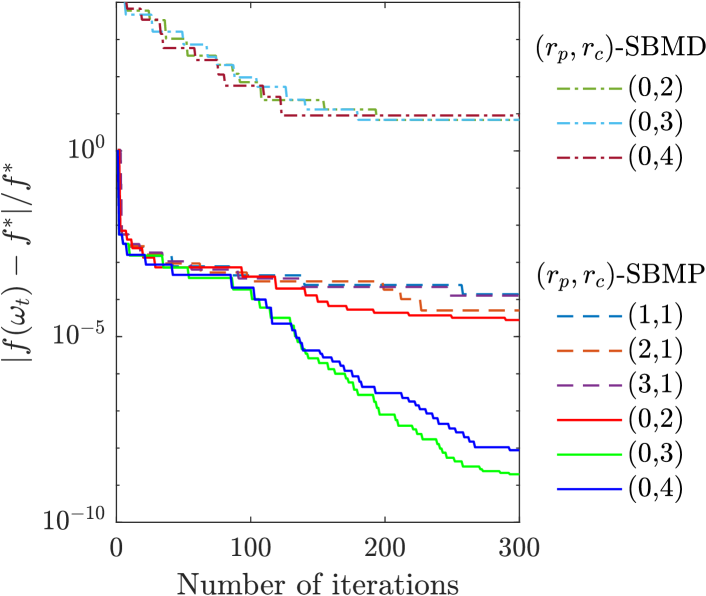
(a) An SDP instance with $\mathrm{rank}(Z^{\star})=3$

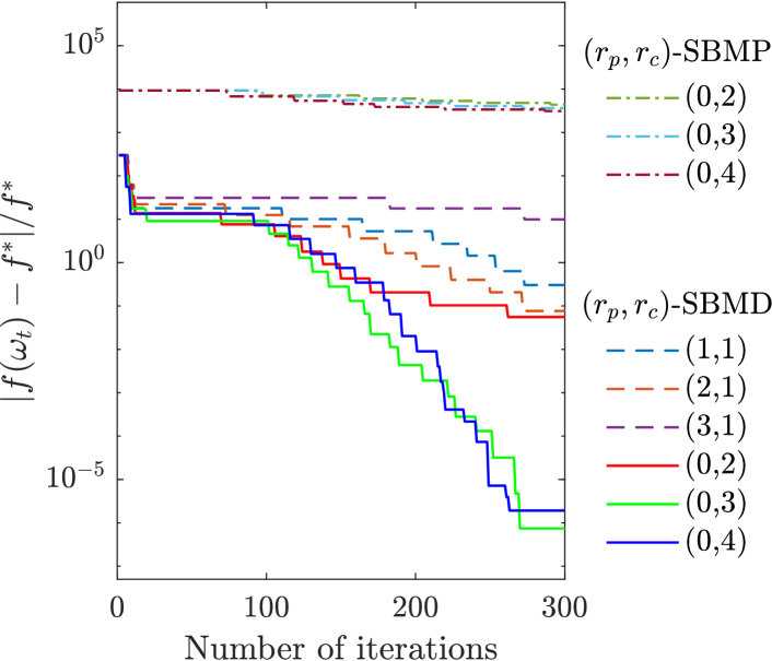
(b) An SDP instance with $\mathrm{rank}(X^{\star})=3$

Figure 1: The relative optimality gap of different choices of $r_{\mathrm{p}}$ and $r_{\mathrm{c}}$ in $(r_{\mathrm{p}},r_{\mathrm{c}})$-SBMP and $(r_{\mathrm{p}},r_{\mathrm{c}})$-SBMD for solving two SDPs with $X\in\mathbb{S}^{1000}_{+}$: the left SDP instance admits a low-rank dual solution $\mathrm{rank}(Z^{\star})=3$ which suits well for $(r_{\mathrm{p}},r_{\mathrm{c}})$-SBMP, while the right SDP instance admits a low-rank primal solution $\mathrm{rank}(X^{\star})=3$ that suits well for $(r_{\mathrm{p}},r_{\mathrm{c}})$-SBMD.

Table 2: Computational results of $(r_{\mathrm{p}},r_{\mathrm{c}})$-SBMP and$(r_{\mathrm{p}},r_{\mathrm{c}})$-SBMD for solving two random SDPs ($n=1000$ and $m=200$) under different values of $r_{\mathrm{p}}$ and $r_{\mathrm{c}}$. “Semi Feasi.” denotes the violation of PSD constraints $\max\{\eta_{2},\eta_{4}\}$, “Affine Feasi.” denotes the violation of affine constraints $\max\{\eta_{1},\eta_{3}\}$, “Dual Gap” denotes the duality gap $\eta_{5}$ in 47, and “Cost Opt.” denotes the cost-value gap $\eta_{\mathrm{c}}={(f(\omega_{t})-f^{\star})}/{f^{\star}}$.

SDP instance	Algorithm	$(r_{\mathrm{p}},r_{\mathrm{c}})$	Semi Feasi.	Affine Feasi.	Dual Gap	Cost Opt.
$\begin{aligned} &\text{Instance 1}\\ &\text{rank}(Z^{\star})=3\end{aligned}$	$(r_{\mathrm{p}},r_{\mathrm{c}})$-SBMD	$(0,2)$	$-7.53\mathrm{e}{-1}$	$1.55\mathrm{e}{-4}$	$4.28\mathrm{e}{-5}$	$13.1$
		$(0,3)$	$-7.59\mathrm{e}{-1}$	$1.54\mathrm{e}{-4}$	$3.62\mathrm{e}{-4}$	$13.1$
		$(0,4)$	$-9.96\mathrm{e}{-1}$	$3.31\mathrm{e}{-4}$	$1.10\mathrm{e}{-4}$	$28.6$
	$(r_{\mathrm{p}},r_{\mathrm{c}})$-SBMP	$(1,1)$	$-3.67\mathrm{e}{-3}$	$3.27\mathrm{e}{-4}$	$1.24\mathrm{e}{-5}$	$1.38\mathrm{e}{-4}$
		$(2,1)$	$-2.92\mathrm{e}{-3}$	$3.18\mathrm{e}{-5}$	$1.03\mathrm{e}{-5}$	$1.02\mathrm{e}{-4}$
		$(3,1)$	$-7.22\mathrm{e}{-3}$	$9.00\mathrm{e}{-6}$	$9.74\mathrm{e}{-7}$	$2.17\mathrm{e}{-4}$
		$(0,2)$	$-3.58\mathrm{e}{-4}$	$2.46\mathrm{e}{-4}$	$5.06\mathrm{e}{-5}$	$3.22\mathrm{e}{-5}$
		$(0,3)$	$-1.17\mathrm{e}{-8}$	$1.57\mathrm{e}{-6}$	$3.38\mathrm{e}{-7}$	$2.14\mathrm{e}{-9}$
		$(0,4)$	$-1.40\mathrm{e}{-7}$	$3.22\mathrm{e}{-6}$	$6.91\mathrm{e}{-7}$	$1.05\mathrm{e}{-8}$
$\begin{aligned} &\text{Instance 2}\\ &\text{rank}(X^{\star})=3\end{aligned}$	$(r_{\mathrm{p}},r_{\mathrm{c}})$-SBMP	$(0,2)$	$-144$	$6.82\mathrm{e}{-1}$	$9.99\mathrm{e}{-1}$	$4801$
		$(0,3)$	$-121$	$5.61\mathrm{e}{-1}$	$9.99\mathrm{e}{-1}$	$4041$
		$(0,4)$	$-106$	$4.58\mathrm{e}{-1}$	$9.99\mathrm{e}{-1}$	$3369$
	$(r_{\mathrm{p}},r_{\mathrm{c}})$-SBMD	$(1,1)$	$-1.80$	$3.11\mathrm{e}{-2}$	$8.21\mathrm{e}{-3}$	$6.34\mathrm{e}{-1}$
		$(2,1)$	$-5.11\mathrm{e}{-1}$	$2.00\mathrm{e}{-2}$	$4.78\mathrm{e}{-3}$	$2.06\mathrm{e}{-1}$
		$(3,1)$	$-4.95\mathrm{e}{-1}$	$4.25\mathrm{e}{-3}$	$4.62\mathrm{e}{-3}$	$17.7$
		$(0,2)$	$-3.04\mathrm{e}{-1}$	$5.47\mathrm{e}{-3}$	$6.74\mathrm{e}{-4}$	$1.03\mathrm{e}{-1}$
		$(0,3)$	$-4.66\mathrm{e}{-6}$	$6.65\mathrm{e}{-5}$	$4.91\mathrm{e}{-5}$	$4.74\mathrm{e}{-6}$
		$(0,4)$	$-9.30\mathrm{e}{-6}$	$6.65\mathrm{e}{-5}$	$1.32\mathrm{e}{-5}$	$3.94\mathrm{e}{-6}$

In all cases, we ran $(r_{\mathrm{p}},r_{\mathrm{c}})$-SBMP and $(r_{\mathrm{p}},r_{\mathrm{c}})$-SBMD for 300 iterations. In this experiment, we also computed the cost value gap as $\eta_{\mathrm{c}}={(f(\omega_{t})-f^{\star})}/{f^{\star}}.$ The convergence behaviors of the cost value gap are illustrated in Figure 1. In Table 2, we list the suboptimality measures for the final iterates, where “Semi Feasi.” denotes the violation of PSD constraints $\max\{\eta_{2},\eta_{4}\}$, “Affine Feasi.” denotes the violation of affine constraints $\max\{\eta_{1},\eta_{3}\}$, “Dual Gap” denotes the duality gap $\eta_{5}$ in 47, and “Cost Opt.” denotes the cost-value gap $\eta_{\mathrm{c}}$. As expected, the value of $r_{\mathrm{c}}$ greatly affects the convergence performance for both $(r_{\mathrm{p}},r_{\mathrm{c}})$-SBMP and $(r_{\mathrm{p}},r_{\mathrm{c}})$-SBMD. In the first SDP with a low-rank dual solution, we observe that $(r_{\mathrm{p}},r_{\mathrm{c}})$-SBMP has a fast convergence behavior when choosing $r_{\mathrm{c}}\geq 3=\text{dim}(\text{null}(X^{\star}))$, while $(r_{\mathrm{p}},r_{\mathrm{c}})$-SBMD has a slow performance in all settings. On the other hand, in the second SDP with a low-rank primal solution, $(r_{\mathrm{p}},r_{\mathrm{c}})$-SBMD enjoys the fast convergence when $r_{\mathrm{c}}\geq 3=\text{dim}(\text{null}(Z^{\star}))$, while $(r_{\mathrm{p}},r_{\mathrm{c}})$-SBMP converges poorly in all different configurations. The numerical results confirm the theoretical convergence results in Theorems 4.2 and 5.2 and our discussions in Section 5.2.

6.3 Max-Cut

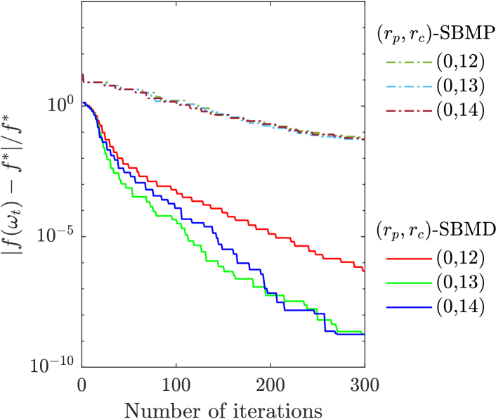
(a) Max-Cut problem with Graph G1

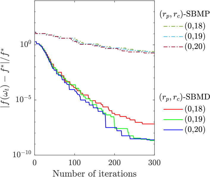
(b) Max-Cut problem with Graph G25

Figure 2: The relative optimality gap of different choices of $r_{\mathrm{p}}$ and $r_{\mathrm{c}}$ in $(r_{\mathrm{p}},r_{\mathrm{c}})$-SBMP and $(r_{\mathrm{p}},r_{\mathrm{c}})$-SBMD for solving SDP relaxations of two Max-Cut problems.

In this experiment, we consider the maximum cut problem, which is a benchmark combinatorial optimization problem. The SDP relaxation is likely to have low-rank primal solutions, for which $(r_{\mathrm{p}},r_{\mathrm{c}})$-SBMD is better suited. Consider an undirected graph $\mathcal{G}(\mathcal{V},\mathcal{E})$ defined by a set of vertices $\mathcal{V}=\{1,2,\ldots,n\}$ and a set of edges $\mathcal{E}\subseteq\mathcal{V}\times\mathcal{V}$, and each edge $\{i,j\}\in\mathcal{E}$ has a weight $w_{ij}=w_{ji}$. The max-cut problem aims to find a maximum cut that separates the vertices into two different groups. This can be formulated as a binary quadratic program [50]

$$\min_{x_{i}^{2}=1,i=1,\ldots,n}\;\;\frac{1}{4}x^{\mathsf{T}}Lx,\\$$ (48)

where $L\in\mathbb{S}^{n}$ is the Laplacian matrix of $\mathcal{G}(\mathcal{V},\mathcal{E})$ defined as $L_{ij}=\sum_{j\neq i}w_{ij}$ if $i=j$, and $L_{ij}=-w_{ij}$ otherwise. A well-known semidefinite relaxation [50] for the Max-Cut problem 48 is

$$\min_{X} \frac{1}{4}\langle L,X\rangle$$ (49)

$$\mathrm{subject\leavevmode\nobreak\ to} X_{ii}=1,\ldots,n,$$

$$X\in\mathbb{S}^{n}_{+}.$$

If the optimal solution of SDP relaxation 49 satisfies $\mathrm{rank}(X^{\star})=1$, then the SDP relaxation 49 is exact and one can recover a globally optimal solution to 48. However, the rank-one solution may not exist. Instead, many max-cut instances admit low-rank optimal solutions: $1<\mathrm{rank}(X^{\star})\ll n$, as observed in [17, Section 1.3.2], [29, Section 5.1]. For these SDP instances, we expect that $(r_{\mathrm{p}},r_{\mathrm{c}})$-SBMD exhibits faster linear convergence when choosing a small value of $r_{\mathrm{c}}$, while $(r_{\mathrm{p}},r_{\mathrm{c}})$-SBMP only has slower sublinear convergence for the same choice of $r_{\mathrm{c}}$.

We run both $(r_{\mathrm{p}},r_{\mathrm{c}})$-SBMP and $(r_{\mathrm{p}},r_{\mathrm{c}})$-SBMD for a fixed number of 300 iterations for two Max-Cut instances G1 and G25 from [57]. There are 800 nodes in graph G1, and 2000 nodes in graph G25, and so the PSD constraints in 49 have a dimension of 800 and 2000, respectively. Despite the large value of $n$, we observed a low rank primal solution $\mathrm{rank}(X^{\star})=12$ for G1 and $\mathrm{rank}(X^{\star})=19$ for G25. Note that the SDP 49 has a constant trace property $\mathop{\bf tr}(X)=n$. Thus, we chose the penalty parameter $\rho=2n+2$ for $(r_{\mathrm{p}},r_{\mathrm{c}})$-SBMD. We can also estimate the penalty parameter for $(r_{\mathrm{p}},r_{\mathrm{c}})$-SBMP as $\rho=2\mathopen{}\mathclose{{}\left(\frac{1}{4}\mathop{\bf tr}(L)-\frac{n}{4}\min\{0,\lambda_{\min}(L)\}}\right)+2$. We set $r_{\mathrm{p}}=0$ since this parameter has little impact on convergence in this case. The other parameters were chosen as those in Section 6.2.

The numerical results are illustrated in Figure 2 and Table 3. In all cases, compared with $(r_{\mathrm{p}},r_{\mathrm{c}})$-SBMP, $(r_{\mathrm{p}},r_{\mathrm{c}})$-SBMD returns solutions with much higher accuracy within the same number of iterations. In particular, since the rank condition 45 is expected to hold, $(r_{\mathrm{p}},r_{\mathrm{c}})$-SBMD shows a faster linear convergence rate, while $(r_{\mathrm{p}},r_{\mathrm{c}})$-SBMP converges to an optimal solution slowly. Again, this is consistent with the theoretical expectation in Section 5.2.

Table 3: Computational results of $(r_{\mathrm{p}},r_{\mathrm{c}})$-SBMP and $(r_{\mathrm{p}},r_{\mathrm{c}})$-SBMD for solving max-cut SDPs 49 under different values of $r_{\mathrm{p}}$ and $r_{\mathrm{c}}$. “Semi Feasi.” denotes the violation of PSD constraints $\max\{\eta_{2},\eta_{4}\}$, “Affine Feasi.” denotes the violation of affine constraints $\max\{\eta_{1},\eta_{3}\}$, “Dual Gap” denotes the duality gap $\eta_{5}$ in 47, and “Cost Opt.” denotes the cost-value gap $\eta_{\mathrm{c}}={(f(\omega_{t})-f^{\star})}/{f^{\star}}$.

Max-cut instance	Algorithm	$(r_{\mathrm{p}},r_{\mathrm{c}})$	Semi Feasi.	Affine Feasi.	Dual Gap	Cost Opt.
$\begin{aligned} &\text{G1}\\ &\text{rank}(X^{\star})=12\\ &n=800\\ &m=800\end{aligned}$	$(r_{\mathrm{p}},r_{\mathrm{c}})$-SBMP	$(0,12)$	$-1.39\mathrm{e}{-2}$	$7.28\mathrm{e}{-2}$	$1.68\mathrm{e}{-2}$	$6.85\mathrm{e}{-2}$
		$(0,13)$	$-1.39\mathrm{e}{-2}$	$6.94\mathrm{e}{-2}$	$1.77\mathrm{e}{-2}$	$5.49\mathrm{e}{-2}$
		$(0,14)$	$-2.36\mathrm{e}{-2}$	$6.63\mathrm{e}{-2}$	$1.47\mathrm{e}{-2}$	$5.97\mathrm{e}{-2}$
	$(r_{\mathrm{p}},r_{\mathrm{c}})$-SBMD	$(0,12)$	$-3.80\mathrm{e}{-6}$	$7.16\mathrm{e}{-4}$	$1.23\mathrm{e}{-5}$	$6.86\mathrm{e}{-7}$
		$(0,13)$	$-2.52\mathrm{e}{-9}$	$2.69\mathrm{e}{-5}$	$4.58\mathrm{e}{-8}$	$2.31\mathrm{e}{-9}$
		$(0,14)$	$-1.69\mathrm{e}{-9}$	$4.42\mathrm{e}{-5}$	$1.83\mathrm{e}{-7}$	$1.97\mathrm{e}{-9}$
$\begin{aligned} &\text{G25}\\ &\text{rank}(X^{\star})=19\\ &n=2000\\ &m=2000\end{aligned}$	$(r_{\mathrm{p}},r_{\mathrm{c}})$-SBMP	$(0,18)$	$-1.27\mathrm{e}{-1}$	$4.73\mathrm{e}{-1}$	$3.88\mathrm{e}{-2}$	$3.07\mathrm{e}{-1}$
		$(0,19)$	$-9.24\mathrm{e}{-2}$	$1.18$	$2.33\mathrm{e}{-1}$	$2.51\mathrm{e}{-1}$
		$(0,20)$	$-8.27\mathrm{e}{-2}$	$6.62\mathrm{e}{-1}$	$1.30\mathrm{e}{-1}$	$2.24\mathrm{e}{-1}$
	$(r_{\mathrm{p}},r_{\mathrm{c}})$-SBMD	$(0,18)$	$-2.17\mathrm{e}{-7}$	$6.34\mathrm{e}{-4}$	$3.63\mathrm{e}{-6}$	$9.37\mathrm{e}{-8}$
		$(0,19)$	$-1.72\mathrm{e}{-9}$	$3.04\mathrm{e}{-6}$	$1.77\mathrm{e}{-8}$	$2.76\mathrm{e}{-9}$
		$(0,20)$	$-2.83\mathrm{e}{-9}$	$2.76\mathrm{e}{-5}$	$2.99\mathrm{e}{-8}$	$3.01\mathrm{e}{-9}$

6.4 Quartic polynomial optimization on a sphere

In our last numerical experiments, we consider SOS relaxations for polynomial optimization, which are likely to admit low-rank dual solutions. We expect that $(r_{\mathrm{p}},r_{\mathrm{c}})$-SBMP is better suited than $(r_{\mathrm{p}},r_{\mathrm{c}})$-SBMD. Our numerical results further show that $(r_{\mathrm{p}},r_{\mathrm{c}})$-SBMP outperforms a set of baseline solvers, including interior-point solvers SDPT3 [40], MOSEK [41], and first-order solvers CDCS [42], SDPNAL+ [16].

Consider a constrained polynomial optimization problem over a sphere $\min_{x\in\mathcal{S}^{n-1}}\;p_{0}(x),$ where $p_{0}(x):\mathbb{R}^{n}\rightarrow\mathbb{R}$ is a polynomial and $\mathcal{S}^{n-1}=\{x\in\mathbb{R}^{n}\mid\|x\|^{2}=1\}$ is the $n$-dimensional unit sphere. This problem is in general NP-hard, but it can be approximated well using the moment/SOS relaxation [35, 36]. In particular, the $k$th-order SOS relaxation is

$$\max_{\gamma,\sigma_{0},\psi_{1}} \quad\gamma$$ (50)

$$\mathrm{subject\leavevmode\nobreak\ to} \quad p_{0}(x)-\gamma-\psi_{1}h(x)=\sigma_{0},$$

$$\quad\sigma_{0}\in\Sigma[x]_{n,2k},\;\psi_{1}\in\mathbb{R}[x]_{n,2(k-\lceil h\rceil)},$$

where $h(x)=\|x\|^{2}-1$, $\lceil h\rceil=\lceil\mathrm{deg}(h)/2\rceil$, $\mathbb{R}[x]_{n,2(k-\lceil h\rceil)}$ denotes the real polynomial in $n$ variables and degree at most $2(k-\lceil h\rceil)$, and $\Sigma[x]_{n,2k}$ denote the cone of SOS polynomials in $\mathbb{R}[x]_{n,2k}$. It is well-known that 50 can be equivalently reformulated into the standard primal SDP in the form P with some extra free variables; see e.g., [35] for details. We observe that these SDPs are likely to admit low-rank dual solutions (this observation is consistent with the flat extension theory on the moment side [36, Theorem 3.7] when it is formulated as a dual SDP).

Motivated by the benchmark problems [58], we consider three instances of 50 in our numerical experiments:

1. Modified Broyden tridiagonal polynomial

   $$q_{1}(x)= \mathopen{}\mathclose{{}\left(\mathopen{}\mathclose{{}\left(3-2x_{1}}\right)x_{1}-2x_{2}+1}\right)^{2}+$$

   $$\sum_{i=2}^{d-1}\mathopen{}\mathclose{{}\left(\mathopen{}\mathclose{{}\left(3-2x_{i}}\right)x_{i}-x_{i-1}-2x_{i+1}+1}\right)^{2}+\mathopen{}\mathclose{{}\left(\mathopen{}\mathclose{{}\left(3-2x_{d}}\right)x_{d}-x_{d-1}+1}\right)^{2}+\mathopen{}\mathclose{{}\left(\sum_{i=1}^{d}x_{i}}\right)^{2}.$$

2. Modified Rosenbrock polynomial $q_{2}(x)=1+\sum_{i=2}^{d}100\mathopen{}\mathclose{{}\left(x_{i}-x_{i-1}^{2}}\right)^{2}+\mathopen{}\mathclose{{}\left(1-x_{i}}\right)^{2}+\mathopen{}\mathclose{{}\left(\sum_{i=1}^{d}x_{i}}\right)^{2}.$

3. Random quartic polynomial $q_{3}(x)=\langle c_{d,4},[x]_{d,4}\rangle,$ where $[x]_{d,4}$ is the standard monomial bases with $d$ variables and degree at most $4$, and $c_{d,4}$ is a randomly generated coefficient vector.

We used the package SOSTOOLS [59] to recast the SOS relaxation 50 with $k=2$ into a standard SDP in the form of P. We tested $(r_{\mathrm{p}},r_{\mathrm{c}})$-SBMP for the above three polynomials with different dimensions (the performance of $(r_{\mathrm{p}},r_{\mathrm{c}})$-SBMD was very poor in our experiments, and we omitted it here). The dimension of the SDP relaxations ranges from $n=496$ to $861$ and $m=45,897$ to $134,889$. Recall in Section 3.1 that we need to choose the penalty parameter $\rho>\mathcal{D}_{Z_{\star}}$ for $(r_{\mathrm{p}},r_{\mathrm{c}})$-SBMP. For SDPs from 50, we can show that any $\rho\geq(1+1)^{2}=4$ is a valid exact penalty parameter (see Lemma E.1) thanks to the unit sphere constraint. We thus chose $\rho=10$ for all cases. The parameters $(r_{\mathrm{p}},r_{\mathrm{c}})$ are chosen as $(0,3),(0,5),$ and $(0,7)$ for three different problems. In our experiments, we ran $(r_{\mathrm{p}},r_{\mathrm{c}})$-SBMP until it reached tolerance $1\mathrm{e}{-4}$.

Table 4: Computational results on the SOS relaxation 50 of quartic polynomial optimization on a sphere: $\epsilon_{\mathrm{p}}$ denotes the primal feasibility, $\epsilon_{\mathrm{d}}$ denotes the primal feasibility, and $\epsilon_{\mathrm{g}}$ denotes the duality gap. Entries marked by oom indicate “out of memory” runtime errors.

Dimension Case Metric SDPT3 [40] MOSEK [41] CDCS [42] SDPNAL+ [16] $(r_{\mathrm{p}},r_{\mathrm{c}})$-SBMP $\begin{subarray}{c}d:\ 30\\ \\ n:\ 496\ \\ \\ m:\ 45,879\ \end{subarray}$ $q_{1}$ $\epsilon_{\mathrm{p}}$ oom $9.2\mathrm{e}{-11}$ $9.9\mathrm{e}{-5}$ $2.1\mathrm{e}{-11}$ $5.9\mathrm{e}{-14}$ $\epsilon_{\mathrm{d}}$ $2.0\mathrm{e}{-9}$ $4.1\mathrm{e}{-5}$ $9.5\mathrm{e}{-5}$ $9.2\mathrm{e}{-5}$ $\epsilon_{\mathrm{g}}$ $5.9\mathrm{e}{-12}$ $9.0\mathrm{e}{-6}$ $1.0\mathrm{e}{-2}$ $6.8\mathrm{e}{-6}$ cost $-25.074$ $-25.073$ $-42.850$ $-25.074$ time $887.1$ $100.9$ $1209$ 17.5 $q_{2}$ $\epsilon_{\mathrm{p}}$ oom $8.2\mathrm{e}{-10}$ $1.5\mathrm{e}{-5}$ $4.7\mathrm{e}{-5}$ $5.4\mathrm{e}{-14}$ $\epsilon_{\mathrm{d}}$ $1.9\mathrm{e}{-8}$ $9.3\mathrm{e}{-5}$ $8.1\mathrm{e}{-5}$ $8.9\mathrm{e}{-5}$ $\epsilon_{\mathrm{g}}$ $2.9\mathrm{e}{-10}$ $3.9\mathrm{e}{-5}$ $6.7\mathrm{e}{-3}$ $5.3\mathrm{e}{-5}$ cost $-32.136$ $-32.137$ $-32.137$ $-32.135$ time $583$ $45.1$ $17.3$ 12.8 $q_{3}$ $\epsilon_{\mathrm{p}}$ oom $9.1\mathrm{e}-{9}$ $1.0\mathrm{e}{-4}$ $3.2\mathrm{e}{-16}$ $1.9\mathrm{e}{-14}$ $\epsilon_{\mathrm{d}}$ $2.0\mathrm{e}{-7}$ $1.5\mathrm{e}{-6}$ $5.2\mathrm{e}{-4}$ $8.7\mathrm{e}{-5}$ $\epsilon_{\mathrm{g}}$ $4.9\mathrm{e}{-9}$ $2.4\mathrm{e}{-6}$ $3.5\mathrm{e}{-3}$ $2.2\mathrm{e}{-5}$ cost $2.023$ $2.023$ $2.021$ $2.023$ time $645.2$ $55.3$ $548.6$ 16.9 $\begin{subarray}{c}d:\ 35\\ \\ n:\ 666\\ \\ m:\ 81,584\end{subarray}$ $q_{1}$ $\epsilon_{\mathrm{p}}$ oom oom $9.6\mathrm{e}{-5}$ $1.1\mathrm{e}{-15}$ $9.9\mathrm{e}{-14}$ $\epsilon_{\mathrm{d}}$ $1.9\mathrm{e}{-5}$ $6.8\mathrm{e}{-5}$ $9.9\mathrm{e}{-5}$ $\epsilon_{\mathrm{g}}$ $2.1\mathrm{e}{-5}$ $2.7\mathrm{e}{-4}$ $9.4\mathrm{e}{-6}$ cost $-30.053$ $-30.070$ $-30.050$ time $289.6$ $3449.4$ 41.4 $q_{2}$ $\epsilon_{\mathrm{p}}$ oom oom $2.2\mathrm{e}{-5}$ $4.2\mathrm{e}{-5}$ $1.3\mathrm{e}{-13}$ $\epsilon_{\mathrm{d}}$ $9.4\mathrm{e}{-5}$ $9.5\mathrm{e}{-5}$ $8.8\mathrm{e}{-5}$ $\epsilon_{\mathrm{g}}$ $7.7\mathrm{e}{-5}$ $2.4\mathrm{e}{-3}$ $2.0\mathrm{e}{-5}$ cost $-37.100$ $-37.221$ $-37.091$ time $112.3$ $100.5$ 42.7 $q_{3}$ $\epsilon_{\mathrm{p}}$ oom oom $1.0\mathrm{e}{-4}$ $9.3\mathrm{e}{-13}$ $1.9\mathrm{e}{-14}$ $\epsilon_{\mathrm{d}}$ $6.9\mathrm{e}{-5}$ $6.5\mathrm{e}{-7}$ $9.4\mathrm{e}{-5}$ $\epsilon_{\mathrm{g}}$ $3.5\mathrm{e}{-5}$ $6.2\mathrm{e}{-3}$ $2.5\mathrm{e}{-6}$ cost $2.121$ $2.039$ $2.121$ time $170.1$ $1208.4$ 44.5 $\begin{subarray}{c}d:\ 40\\ \\ n:\ 861\\ \\ m:\ 134,889\end{subarray}$ $q_{1}$ $\epsilon_{\mathrm{p}}$ oom oom $1.0\mathrm{e}{-4}$ $3.6\mathrm{e}{-12}$ $7.4\mathrm{e}{-14}$ $\epsilon_{\mathrm{d}}$ $3.2\mathrm{e}{-6}$ $1.0\mathrm{e}{-4}$ $9.6\mathrm{e}{-5}$ $\epsilon_{\mathrm{g}}$ $1.4\mathrm{e}{-5}$ $4.9\mathrm{e}{-2}$ $5.2\mathrm{e}{-6}$ cost $-35.037$ $-47.792$ $-35.034$ time $738.9$ $1881.1$ 84.8 $q_{2}$ $\epsilon_{\mathrm{p}}$ oom oom $1.7\mathrm{e}{-5}$ $3.3\mathrm{e}{-14}$ $1.3\mathrm{e}{-13}$ $\epsilon_{\mathrm{d}}$ $9.3\mathrm{e}{-5}$ $9.9\mathrm{e}{-5}$ $5.5\mathrm{e}{-5}$ $\epsilon_{\mathrm{g}}$ $5.8\mathrm{e}{-5}$ $2.8\mathrm{e}{-5}$ $1.6\mathrm{e}{-5}$ cost $-42.041$ $-41.997$ $-42.050$ time $254.9$ $187.6$ 82.1 $q_{3}$ $\epsilon_{\mathrm{p}}$ oom oom $1.0\mathrm{e}{-4}$ $9.1\mathrm{e}{-16}$ $2.0\mathrm{e}{-14}$ $\epsilon_{\mathrm{d}}$ $1.6\mathrm{e}{-6}$ $7.5\mathrm{e}{-5}$ $8.2\mathrm{e}{-5}$ $\epsilon_{\mathrm{g}}$ $4.9\mathrm{e}{-5}$ $2.4\mathrm{e}{-3}$ $1.0\mathrm{e}{-4}$ cost $2.681$ $2.695$ $2.681$ time $144.5$ $1339.6$ 93.1

To further demonstrate the performance of $(r_{\mathrm{p}},r_{\mathrm{c}})$-SBMP, we compare it with SDPT3 [40], MOSEK [41], CDCS [42], SDPNAL+ [16]. For SDPT3 and MOSEK, we used their default parameters. For CDCS, we use the sos solver with a maximum 10,000 iterations with tolerance $1\mathrm{e}{-4}$, and this sos option is customized for solving SDPs from SOS relaxations (by exploiting a property called partial orthogonality [60]). For SDPNAL+, we used $1\mathrm{e}{-4}$ as the tolerance, turn off their stagnation detection, and run it using their default parameter with a maximum of 20,000 iterations and a maximum of 10,000 seconds runtime.

The computational results are listed in Table 4. To be consistent with other solvers, we report the cost value, time consumption, primal feasibility, dual feasibility, and duality gap (see 47) of the final outcome, i.e.,

$$\epsilon_{\mathrm{p}}=\eta_{1},\;\epsilon_{\mathrm{d}}=\eta_{3},\;\epsilon_{\mathrm{g}}=\eta_{5}.$$

As we can see in Table 4, our algorithm $(r_{\mathrm{p}},r_{\mathrm{c}})$-SBMP solves all SDP instances to the desired accuracy within a reasonable time, and it consistently outperforms the baseline solvers. For the interior-point solvers, $\sf{SDPT3}$ runs out of memory in all cases on our computer. $\sf{MOSEK}$ was able to return solutions of high accuracy for medium-size problems ($d=30$) but took more time consumption. $\sf{MOSEK}$ also encountered memory issues for larger instances ($d\geq 35$). For the first-order solvers, CDCS solved all tested problems with medium accuracy, but the runtime was worse than $(r_{\mathrm{p}},r_{\mathrm{c}})$-SBMP (indeed, our algorithm $(r_{\mathrm{p}},r_{\mathrm{c}})$-SBMP was one order of magnitude faster than CDCS in some cases); the solver SDPNAL+ solved all SDPs to the desired accuracy for the measures $\epsilon_{\mathrm{p}}$ and $\epsilon_{\mathrm{d}}$, while the duality gap $\epsilon_{\mathrm{g}}$ remains unsatisfactory. We note that the design of SDPNAL+ does not consider the duality gap $\epsilon_{\mathrm{g}}$ as a stopping criterion. This partially explains the poor performance of the duality gap $\epsilon_{\mathrm{g}}$ in the final iterate.

7 Conclusion

In this paper, we have presented an overview and comparison of spectral bundle methods for solving primal and dual SDPs. All the existing results focus on solving dual SDPs. We have established a family of spectral bundle methods for solving primal SDPs directly. The algorithm developments mirror the elegant duality between primal and dual SDPs. We have presented the sublinear convergence rates for this family of spectral bundle methods and shown that the algorithm enjoys linear convergence with proper parameter choice and low-rank dual solutions. The convergence behaviors and computational complexity of spectral bundle methods for both primal and dual SDPs are in general similar, but they have different features. It is clear that the existing spectral bundle methods are well-suited for SDPs with low-rank primal solutions, and our new spectral bundle method works well for SDPs with low-rank dual solutions. These theoretical findings are supported by a range of large-scale numerical experiments. We have further demonstrated that our new spectral bundle method achieves state-of-the-art efficiency and scalability when solving the SDP relaxations from polynomial optimization.

Potential future directions include incorporating other types of constraints (such as nonnegative, second-order cone constraints, etc.), considering second-order information [33] for the lower approximation, and analyzing the algorithm performance when the subproblem 24 is solved inexactly [61]. Finally, we remark that our current prototype implementation shows promising numerical performance, and it would also be very interesting to further develop reliable and efficient open-source implementations of these spectral bundle methods.

Appendix

The appendix is divided into five parts:

1. Appendix A extends the convergence results of generic bundle methods for unconstrained optimization in [39] to constrained convex optimization. We present the adaptions required to prove Lemma 2.2;

2. Appendix B presents some technical proofs in Section 3, i.e., the exact penalization for primal and dual SDPs;

3. Appendix C presents some computation details in $(r_{\mathrm{p}},r_{\mathrm{c}})$-SBMP and $(r_{\mathrm{p}},r_{\mathrm{c}})$-SBMD;

4. Appendix D completes the technical proofs for the convergence guarantees of $(r_{\mathrm{p}},r_{\mathrm{c}})$-SBMP, i.e., Theorems 4.1 and 4.2;

5. Appendix E presents further details of our numerical experiments in Section 6, including the generation of random SDPs and the exact penalty parameter in SOS optimizations on a sphere.

Appendix A Bundle methods for constrained convex optimization

In this section, we show that the three conditions 9a, 9b and 9c ensure the convergence of the bundle method in Algorithm 1 to solve the constrained convex optimization problem 5. We restate 5 below for convenience,

$$f^{\star}=\min_{x\in\mathcal{X}_{0}}\quad f(x),$$ (A.1)

where $f:\mathbb{R}^{n}\rightarrow\mathbb{R}$ is convex but not necessarily differentiable and $\mathcal{X}_{0}\subseteq\mathbb{R}^{n}$ is a closed convex set.

The analysis in [39, Theorem 2.1 and 2.3] focuses on unconstrained convex optimization with $\mathcal{X}_{0}=\mathbb{R}^{n}$ in A.1. We here clarify the minor extension of their analysis to the constrained case with a closed convex set $\mathcal{X}_{0}$. We present the adaptions to prove Lemma 2.2 in the main text. Specifically, we only need to establish the constrained versions of [39, Lemma 5.1, 5.2, and 5.3], which are given in Lemma A.1, A.2 and A.3 below. Then, the proof of Lemma 2.2 follows the same arguments in [39, Section 5]. Following the notations in [39], at iteration $k$, we define the proximal gap by

$$\Delta_{k}:=f(\omega_{k})-\mathopen{}\mathclose{{}\left(f(\bar{x}_{k+1})+\frac{\alpha}{2}\|\bar{x}_{k+1}-\omega_{k}\|^{2}}\right),$$

where $\bar{x}_{k+1}=\operatorname*{\arg\!\min}_{x\in\mathcal{X}_{0}}\mathopen{}\mathclose{{}\left\{f(x)+\frac{\alpha}{2}\|x-\omega_{k}\|^{2}}\right\}$ and $\omega_{k}$ is the reference point. Note that $\bar{x}_{k+1}$ is obtained using the original $f$ rather than the lower approximation model $\hat{f}_{k}$.

Lemma A.1 (Descent steps attain decrease proportionally to the proximal gap).

A descent step at iteration $k$ satisfies

$$f(\omega_{k+1})\leq f(\omega_{k})-\beta\Delta_{k}.$$

Proof.

The proof is the same as in [39, Lemma 5.1]. We omit the details. ∎

Lemma A.2 (The number of consecutive null steps is bounded by the proximal gap).

A descent step, at iteration $k$, followed by $T$ consecutive null steps has at most

$$T\leq\frac{8G_{k+1}^{2}}{(1-\beta)^{2}\alpha\Delta_{k+T}},$$

where $G_{k+1}=\sup\{\|g_{t+1}\|\mid k\leq t\leq k+T\}$. If $f$ is $M$-Lipschitz, the condition simplifies to

$$T\leq\dfrac{8M^{2}}{(1-\beta)^{2}\alpha\Delta_{k+T}}.$$

Proof.

The proof is essentially the same that in [39, Lemma 5.2]. Consider some descent step $k$, followed by $T$ consecutive null step. Define the proximal subproblem gap at $k<t\leq k+T$ by

$$\widetilde{\Delta}_{t}:=f(\omega_{k+1})-\mathopen{}\mathclose{{}\left(\hat{f}_{t}(x_{t+1}^{\star})+\frac{\alpha}{2}\|x_{t+1}^{\star}-\omega_{k+1}\|^{2}}\right).$$

Note that every null step has the same reference point $\omega_{k+1}$. The core of this proof is to show the inequality

$$\widetilde{\Delta}_{t+1} \leq\widetilde{\Delta}_{t}-\frac{(1-\beta)^{2}\alpha\widetilde{\Delta}_{t}^{2}}{8G_{k+1}^{2}}.$$ (A.2)

Before proving this inequality, let us show how it completes the proof first. After $T$ consecutive null steps, the lower bound $\hat{f}_{k+T}(\cdot)\leq f(\cdot)$ in 9a ensures that $\widetilde{\Delta}_{k+T}\geq\Delta_{k+T}$. Thus, to bound $T$, it is sufficient to show that the reversed inequality $\widetilde{\Delta}_{k+T}<\Delta_{k+T}$ holds. Indeed, upon applying the result in [39, Lemma A.1.] that bounds the number of steps for a recursive relation and setting the target accuracy $\epsilon=\Delta_{k+T}$ (note that $\Delta_{k+T}=\Delta_{k+1}$), we conclude the number of consecutive null steps $T$ is at most

$$T\leq\frac{8G_{k+1}^{2}}{(1-\beta)^{2}\alpha\Delta_{k+T}}.$$

Now, let us focus on the derivation of A.2. Consider some null step $k<t\leq k+T$. We define the necessary lower bound given by 9b and 9c as

$$\tilde{f}_{t+1}(x):=\max\mathopen{}\mathclose{{}\left\{\hat{f}_{t}(x_{t+1}^{\star})+\langle s_{t+1},x-x_{t+1}^{\star}\rangle,\ f(x_{t+1}^{\star})+\langle g_{t+1},x-x_{t+1}^{\star}\rangle}\right\}\leq\hat{f}_{t+1}(x),\quad\forall x\in\mathcal{X}_{0},$$

and the solution of a proximal step made by $\tilde{f}_{t+1}(x)$ as $y_{t+2}=\operatorname*{\arg\!\min}_{x\in\mathcal{X}_{0}}\mathopen{}\mathclose{{}\left\{\tilde{f}_{t+1}(x)+\frac{\alpha}{2}\|x-\omega_{k+1}\|^{2}}\right\}$. It admits the analytical solution

$$\theta_{t+1} =\min\mathopen{}\mathclose{{}\left\{1,\frac{\alpha\mathopen{}\mathclose{{}\left(f(x_{t+1}^{\star})-\hat{f}_{t}(x_{t+1}^{\star})}\right)}{\|g_{t+1}-s_{t+1}\|^{2}}}\right\},$$

$$y_{t+2} =\omega_{k+1}-\frac{1}{\alpha}\mathopen{}\mathclose{{}\left(\theta_{t+1}g_{t+1}+(1-\theta_{t+1})s_{t+1}+\hat{h}_{t+1}}\right),$$

where $\hat{h}_{t+1}\in\mathcal{N}_{\mathcal{X}_{0}}(y_{t+2})$. Hence, the objective of the proximal subproblem can be lower bounded by

$$f(x_{t+2}^{\star})+\frac{\alpha}{2}\|x_{t+2}^{\star}-\omega_{k+1}\|^{2}$$

$$\geq \;\tilde{f}_{t+1}(x_{t+2}^{\star})+\frac{\alpha}{2}\|x_{t+2}^{\star}-\omega_{k+1}\|^{2}$$

$$\geq \;\tilde{f}_{t+1}(y_{t+2})+\frac{\alpha}{2}\|y_{t+2}-\omega_{k+1}\|^{2}$$

$$\geq \;\theta_{t+1}(\hat{f}_{t}(x_{t+1}^{\star})+\langle s_{t+1},y_{t+2}-x_{t+1}^{\star}\rangle)+(1-\theta_{t+1})(f(x_{t+1}^{\star})+\langle g_{t+1},y_{t+2}-x_{t+1}^{\star}\rangle)+\frac{\alpha}{2}\|y_{t+2}-\omega_{k+1}\|^{2}$$

$$= \;f(x_{t+1}^{\star})+\theta_{t+1}\mathopen{}\mathclose{{}\left(f(x_{t+1}^{\star})-\hat{f}_{t}(x_{t+1}^{\star})}\right)-\frac{\theta_{t+1}^{2}}{2\alpha}\|g_{t+1}-s_{t+1}\|^{2}+\frac{\alpha}{2}\|x_{t+1}^{\star}-\omega_{k+1}\|^{2}+\frac{1}{2\alpha}\mathopen{}\mathclose{{}\left\|\hat{h}_{t+1}}\right\|^{2}$$

$$\geq \;f(x_{t+1}^{\star})+\theta_{t+1}\mathopen{}\mathclose{{}\left(f(x_{t+1}^{\star})-\hat{f}_{t}(x_{t+1}^{\star})}\right)-\frac{\theta_{t+1}^{2}}{2\alpha}\|g_{t+1}-s_{t+1}\|^{2}+\frac{\alpha}{2}\|x_{t+1}^{\star}-\omega_{k+1}\|^{2},$$

where the equality uses the definition of $y_{t+2}$ and the fact that

$$y_{t+2}=x_{t+1}^{\star}-\frac{1}{\alpha}\mathopen{}\mathclose{{}\left(\hat{h}_{t+1}+\theta_{t+1}(g_{t+1}-s_{t+1})}\right)$$

since $x_{t+1}^{\star}=\omega_{k+1}-\frac{1}{\alpha}s_{t+1}$ by the optimality condition of the subproblem $\operatorname*{\arg\!\min}_{x\in\mathcal{X}_{0}}\mathopen{}\mathclose{{}\left\{\hat{f}_{t}(x)+\frac{\alpha}{2}\|x-\omega_{k+1}\|^{2}}\right\}$ at iteration $t$. Thus, we have

$$\widetilde{\Delta}_{t+1}\leq\widetilde{\Delta}_{t}-\mathopen{}\mathclose{{}\left(\theta_{t+1}\mathopen{}\mathclose{{}\left(f(x_{t+1}^{\star})-\hat{f}_{t}(x_{t+1}^{\star})}\right)-\frac{\theta_{t+1}^{2}}{2\alpha}\|g_{t+1}-s_{t+1}\|^{2}}\right).$$

The amount of decrease above can be lower bounded as follows

$$\theta_{t+1}\mathopen{}\mathclose{{}\left(f(x_{t+1}^{\star})-\hat{f}_{t}(x_{t+1}^{\star})}\right)-\frac{\theta_{t+1}^{2}}{2\alpha}\|g_{t+1}-s_{t+1}\|^{2}$$

$$\;\geq\frac{1}{2}\min\mathopen{}\mathclose{{}\left\{f(x_{t+1}^{\star})-\hat{f}_{t}(x_{t+1}^{\star}),\frac{\alpha\mathopen{}\mathclose{{}\left(f(x_{t+1}^{\star})-\hat{f}_{t}(x_{t+1}^{\star})}\right)^{2}}{\|g_{t+1}-s_{t+1}\|^{2}}}\right\}$$

$$\;\geq\frac{1}{2}\min\mathopen{}\mathclose{{}\left\{(1-\beta)\widetilde{\Delta}_{t},\frac{\alpha(1-\beta)^{2}\widetilde{\Delta}_{t}^{2}}{\|g_{t+1}-s_{t+1}\|^{2}}}\right\}$$

$$\;\geq\frac{1}{2}\min\mathopen{}\mathclose{{}\left\{(1-\beta)\widetilde{\Delta}_{t},\frac{\alpha(1-\beta)^{2}\widetilde{\Delta}_{t}^{2}}{2\|g_{t+1}\|^{2}+2\|s_{t+1}\|^{2}}}\right\},$$

where the first inequality uses the definition of $\theta_{t+1}$, the second inequality uses the definition of the null step, and the third inequality uses Young’s inequality. It is clear that both components in the minimum above are non-negative and we have a weaker result that $\widetilde{\Delta}_{t+1}$ is non-increasing. Upon further utilizing the relation $\|s_{t+1}\|^{2}\leq 2\alpha\widetilde{\Delta}_{t}\leq G^{2}_{k+1}$ (which will be shown later), the decrease bound above is at least

$$=\frac{1}{2}\min\mathopen{}\mathclose{{}\left\{(1-\beta)\widetilde{\Delta}_{t},\frac{\alpha(1-\beta)^{2}\widetilde{\Delta}_{t}^{2}}{2\|g_{t+1}\|^{2}+2\|s_{t+1}\|^{2}}}\right\}$$

$$\geq\frac{1}{2}\min\mathopen{}\mathclose{{}\left\{2\frac{\alpha(1-\beta)\widetilde{\Delta}_{t}^{2}}{G_{k+1}^{2}},\frac{\alpha(1-\beta)^{2}\widetilde{\Delta}_{t}^{2}}{4G_{k+1}^{2}}}\right\}$$

$$\geq\frac{\alpha(1-\beta)^{2}\widetilde{\Delta}_{t}^{2}}{8G_{k+1}^{2}}$$

$$\geq\frac{\alpha(1-\beta)^{2}\widetilde{\Delta}_{t}^{2}}{8M^{2}},$$

where the last inequality applies the observation that the subgradient $\|G_{k+1}\|$ is uniformly upper bounded by the $M$ as $f$ is $M$-Lipschitz. Hence, we conclude that $\widetilde{\Delta}_{t+1}\leq\widetilde{\Delta}_{t}-\frac{\alpha(1-\beta)^{2}\widetilde{\Delta}_{t}^{2}}{8M^{2}}.$

We then show the inequality $\|s_{t+1}\|^{2}\leq 2\alpha\widetilde{\Delta}_{t}\leq G^{2}_{k+1}$. By the facts that $\hat{f}_{t}(\cdot)+\frac{\alpha}{2}\|\cdot-\omega_{k+1}\|^{2}$ is $\alpha$ strongly convex and that the minimizer $x_{t+1}^{\star}$ is unique, there exists a $h_{t}\in\mathcal{N}_{\mathcal{X}_{0}}(x_{t+1}^{\star})$ and $v_{t}\in\partial\hat{f}_{t}(x_{t+1}^{\star})+\alpha(x_{t+1}^{\star}-\omega_{k+1})$ such that $0=v_{t}+h_{t}$. It follows from the first-order condition of a strongly convex function that

$$\hat{f}_{t}(\omega_{k+1}) \geq\hat{f}_{t}(x_{t+1}^{\star})+\frac{\alpha}{2}\|x_{t+1}^{\star}-\omega_{k+1}\|^{2}-\langle h_{t},\omega_{k+1}-x_{t+1}^{\star}\rangle+\frac{\alpha}{2}\|x_{t+1}^{\star}-\omega_{k+1}\|^{2}$$

$$\geq\hat{f}_{t}(x_{t+1}^{\star})+\frac{\alpha}{2}\|x_{t+1}^{\star}-\omega_{k+1}\|^{2}+\frac{\alpha}{2}\|x_{t+1}^{\star}-\omega_{k+1}\|^{2},$$

where the second inequality uses the definition of normal cone $\langle h_{t},y-x_{t+1}^{\star}\rangle\leq 0,\forall y\in\mathcal{X}_{0}.$ Using the lower bound property $\hat{f}_{t}(\omega_{k+1})\leq f(\omega_{k+1})$, we have

$$\frac{\alpha}{2}\|x_{t+1}^{\star}-\omega_{k+1}\|^{2}\leq f(\omega_{k+1})-\mathopen{}\mathclose{{}\left(\hat{f}_{t}(x_{t+1}^{\star})+\frac{\alpha}{2}\|x_{t+1}^{\star}-\omega_{k+1}\|^{2}}\right)=\widetilde{\Delta}_{t}\leq\widetilde{\Delta}_{k+1},$$

where the second inequality comes from the fact that $\widetilde{\Delta}_{t}$ is non-increasing.

By the construction of the lower approximation model at step $k+1$ and Young’s inequality, we know

$$\hat{f}_{k+1}(x^{\star}_{k+2}) \geq f(\omega_{k+1})+\langle g_{k+1},x^{\star}_{k+2}-\omega_{k+1}\rangle$$

$$\geq f(\omega_{k+1})-\frac{1}{2}\mathopen{}\mathclose{{}\left(\frac{\|g_{k+1}\|^{2}}{\alpha}+\alpha\|x^{\star}_{k+2}-\omega_{k+1}\|^{2}}\right),$$

where $g_{k+1}\in\partial f(\omega_{k+1}).$ Combining the above inequality and the definition $\widetilde{\Delta}_{k+1}$, we get the relationship

$$\frac{\alpha}{2}\|x_{t+1}^{\star}-\omega_{k+1}\|^{2}\leq\widetilde{\Delta}_{t}\leq\widetilde{\Delta}_{k+1}\leq\frac{1}{2\alpha}\|g_{k+1}\|^{2},$$

which implies $\|s_{t+1}\|^{2}=\alpha^{2}\|x_{t+1}^{\star}-\omega_{k+1}\|^{2}\leq 2\alpha\widetilde{\Delta}_{t}^{2}\leq 2\alpha\widetilde{\Delta}_{k+1}\leq\|g_{k+1}\|^{2}\leq G_{k+1}^{2}$.

∎

Lemma A.3 (Lower bound on the proximal gap).

Fix a minimizer $x^{\star}$ in A.1 and let $\omega_{k}\in\mathbb{R}^{n}\backslash\{x^{\star}\}$, the proximal gap is lower bounded by

$$\Delta_{k}\geq\begin{cases}\dfrac{1}{2\alpha}\mathopen{}\mathclose{{}\left(\dfrac{f(\omega_{k})-f(x^{*})}{\|\omega_{k}-x^{*}\|}}\right)^{2},&\text{ if }f(\omega_{k})-f(x^{*})\leq\alpha\|\omega_{k}-x^{*}\|^{2},\\ f(\omega_{k})-f(x^{*})-\dfrac{\alpha}{2}\|\omega_{k}-x^{*}\|^{2},&\text{ otherwise.}\end{cases}$$

Proof.

This follows [38, Lemma 7.12] exactly and we omit the proof here. ∎

The proof of Lemma 2.2 follows the same arguments in [39, Section 5] via combining Lemma A.1, A.2 and A.3. Indeed,

• Lemma A.1 gives the progress made in the descent step with the relation to the proximal gap;

• Lemma A.2 shows that the maximum number of null steps between two descent steps depends on the proximal gap; and

• Lemma A.3 shows the lower bound on the proximal gap.

As a result, by the lower bound on the proximal gap given in Lemma A.3, the number of null steps between two descent steps can be bounded using Lemma A.2. Combining Lemma A.1 and A.3, we can achieve the maximum number of descent steps to achieve the desired accuracy. Finally, considering both the maximum number of null steps and descent steps renders the maximum number of total steps to achieve the desired accuracy, which gives the convergence results in Lemma 2.2. We refer interested readers to [39, Section 5] for more details.

Appendix B Technical proofs in Section 3

B.1 Proof of Proposition 3.1

We first recall two technical lemmas: the first one is the KKT optimality condition for the primal and dual SDPs P and D, which is shown in Lemma 2.1, and the second one is the computation of the subdifferential of the maximal eigenvalue of symmetric matrices.

Lemma B.1 ([49, Theorem 2]).

Given a symmetric matrix $A\in\mathbb{S}^{n}$. Suppose its maximal eigenvalue $\lambda_{\max}(A)$ has multiplicity $t$. Then, we have

$$\partial\lambda_{\max}(A)=\{QUQ^{\mathsf{T}}\mid U\in\mathbb{S}^{t}_{+},\mathop{\bf tr}(U)=1\},$$

where the columns of $Q\in\mathbb{R}^{n\times t}$ forms an orthonormal set of the eigenvectors for $\lambda_{\max}(A)$.

We are now ready to prove Proposition 3.1.

Proof.

Upon denoting $\mathcal{X}_{0}=\{X\in\mathbb{S}^{n}\,|\,\langle A_{i},X\rangle=b_{i},\,i=1,\ldots,m\}$, it is easy to see that the primal SDP P is equivalent to

$$\min_{X} \langle C,X\rangle$$ (B.1)

$$\mathrm{subject\leavevmode\nobreak\ to} \lambda_{\max}(-X)\leq 0,$$

$$X\in\mathcal{X}_{0},$$

where we have applied the fact that $X\succeq 0\Leftrightarrow-X\preceq 0\Leftrightarrow\lambda_{\max}(-X)\leq 0$. Theorem 2.1 ensures that the penalty form 12 is equivalent to B.1 if we choose $\rho>\rho_{0}$ with $\rho_{0}=\sup_{\lambda\in\Lambda}|\lambda|$, where $\Lambda\subset\mathbb{R}$ is the set of Lagrange multipliers associated with the inequality $\lambda_{\max}(-X)\leq 0$.

Denote $\tilde{\Lambda}=\{\mathop{\bf tr}(Z^{\star})\in\mathbb{R}\mid(y^{\star},Z^{\star})\in\mathcal{D}^{\star}\}$, where $\mathcal{D}^{\star}$ is the set of dual optimal solutions to D. We only need to show that $\tilde{\Lambda}=\Lambda$. To see this, we start with the KKT optimality condition for B.1, i.e.,

$$0\in C+\alpha\partial(\lambda_{\max}(-X^{\star}))+N_{\mathcal{X}_{0}}(X^{\star})\;\;\Longleftrightarrow\;\;0\in C+\alpha\partial(\lambda_{\max}(-X^{\star}))-\sum_{i=1}^{m}A_{i}y_{i},$$ (B.2a)

$$\alpha\lambda_{\max}(-X^{\star})=0,\quad\alpha\geq 0,\quad\lambda_{\max}(-X^{\star})\leq 0,\quad X^{\star}\in\mathcal{X}_{0},$$ (B.2b)

where $\mathcal{N}_{\mathcal{X}_{0}}(X^{\star}):=\{X\in\mathbb{S}^{n}\,|\,\langle X,Y-X^{\star}\rangle\leq 0,\forall Y\in\mathcal{X}_{0}\}$ denotes the normal cone to $\mathcal{X}_{0}$ at $X^{\star}$, and we have used the fact that $\mathcal{N}_{\mathcal{X}_{0}}(X^{\star})=\{\sum_{i=1}^{m}A_{i}y_{i}\in\mathbb{S}^{n}\,|\,y\in\mathbb{R}^{m}\}$ since $\mathcal{X}_{0}=\{X\in\mathbb{S}^{n}\,|\,\langle A_{i},X\rangle=b_{i},\,i=1,\ldots,m\}$ is an affine space. The set of Lagrange multipliers $\Lambda$ associated with the inequality $\lambda_{\max}(-X)\leq 0$ is all $\alpha$ satisfying B.2a and B.2b.

Our proof is divided into two steps.

• We first prove that $\tilde{\Lambda}\subseteq\Lambda$. For any dual optimal solution $(y^{\star},Z^{\star})\in\mathcal{D}^{\star}$, let the corresponding primal optimal solution be $X^{\star}$. It suffices to show that $\alpha=\mathop{\bf tr}(Z^{\star})$, $y^{\star}$, and $X^{\star}$ satisfy B.2a and B.2b.

  If $X^{\star}$ is strictly positive definite, then $Z^{\star}=0$ according to Lemma 2.1. Then $X^{\star}$, $\alpha=\mathop{\bf tr}(Z^{\star})=0$, and $C-\sum_{i=1}^{m}A_{i}y_{i}^{\star}=0$ naturally satisfy B.2a-B.2b.

  If $X^{\star}$ is positive semidefinite with $\lambda_{\max}(-X^{\star})=-\lambda_{\min}(X^{\star})=0$, then $\alpha=\mathop{\bf tr}(Z^{\star})\geq 0$ naturally satisfies B.2b. Denote the multiplicity of $\lambda_{\min}(X^{\star})=0$ as $r$, and the corresponding set of orthonormal eigenvectors as the columns of $P\in\mathbb{R}^{n\times r}$. Via a classical chain rule (see e.g.,[62, Theorem XI.3.2.1]) and Lemma B.1, the subdifferential of $\lambda_{\max}(-X^{\star})$ is

  $$\partial\lambda_{\max}(-X^{\star})=\{-PUP^{\mathsf{T}}\in\mathbb{S}^{n}\,|\,U\in\mathbb{S}^{r}_{+},\mathop{\bf tr}(U)=1\}.$$

  By Lemma 2.1, it is not difficult to see that $Z^{\star}\in\{\mathop{\bf tr}(Z^{\star})\times PUP^{\mathsf{T}}\,|\,U\in\mathbb{S}^{r}_{+},\mathop{\bf tr}(U)=1\}$, which indicates

  $$C-\sum_{i=1}^{m}A_{i}y_{i}^{\star}=Z^{\star}\in-\mathop{\bf tr}(Z^{\star})\partial\lambda_{\max}(-X^{\star}).$$

  Thus, $\alpha=\mathop{\bf tr}(Z^{\star})$, $y^{\star}$, and $X^{\star}$ also satisfy B.2a.

• We then prove $\Lambda\subseteq\tilde{\Lambda}$. It suffices to show that for any $\alpha,y\in\mathbb{R}^{m},X^{\star}$ satisfying B.2a-B.2b, the points $X^{\star},(y,Z=C-\sum_{i=1}^{m}A_{i}y_{i})$ are a pair of primal and dual optimal solutions to the SDPs P and D (note that B.2a implies that $\mathop{\bf tr}(Z)=\mathop{\bf tr}(C-\sum_{i=1}^{m}A_{i}y_{i})=\alpha$).

  By definition, it is clear that $X^{\star},y,Z=C-\sum_{i=1}^{m}A_{i}y_{i}$ are primal and dual feasible, i.e.,

  $$\langle A_{i},X^{\star}\rangle=b_{i},i=1,\ldots,m,\quad\sum_{i=1}^{m}A_{i}y_{i}+Z=C,\quad X^{\star}\succeq 0,\quad Z\succeq 0.$$

  By Lemma 2.1, we only need to show that the complementarity slackness $X^{\star}Z=0$ also holds. If $\lambda_{\max}(-X^{\star})<0$, then $\alpha=0$ by B.2b. Thus, we have $Z=C-\sum_{i=1}^{m}A_{i}y_{i}\in-\alpha\partial\lambda_{\max}(-X^{\star})=\{0\},$ leading to $X^{\star}Z=0$. If $\lambda_{\max}(-X^{\star})=0$ with multiplicity $r$, then $PUP^{\mathsf{T}}\times X^{\star}=0,\forall U\in\mathbb{S}^{r}$, where the columns of $P\in\mathbb{R}^{n\times r}$ forms an orthogonal set of the eigenvectors for $\lambda_{\max}(-X^{\star})$. Combining this fact with the definition $Z=C-\sum_{i=1}^{m}A_{i}y_{i}\in-\alpha\partial\lambda_{\max}(-X^{\star})$, we also have $X^{\star}Z=0$. Therefore, the points $X^{\star},y,Z=C-\sum_{i=1}^{m}A_{i}y_{i}$ satisfy the KKT condition for P and D.

Therefore, we have established that $\tilde{\Lambda}=\Lambda$. Together with Theorem 2.1, this completes the proof. ∎

B.2 Constant trace property in primal and dual SDPs

In this subsection, we give a detailed derivation for the penalized primal/dual problem when the feasible set of P and D implies a constant trace constraint on the decision variables $X$ and $Z$, i.e. $\mathop{\bf tr}(X)=k$ and $\mathop{\bf tr}(Z)=k$ for some $k>0$.

B.2.1.    Constant trace in primal SDPs: Derivation of 18

Without loss of generality, we can add the explicit constant trace constraint $\mathop{\bf tr}(X)=k$ to P, leading to

$$\min_{X} \langle C,X\rangle$$

$$\mathrm{subject\leavevmode\nobreak\ to} \langle A_{i},X\rangle=b_{i},\quad i=1,\ldots,m,$$

$$\langle I,X\rangle=k,$$

$$X\in\mathbb{S}^{n}_{+}.$$

Then, the corresponding Lagrangian dual problem reads as

$$\max_{y,t} b^{\mathsf{T}}y+tk$$ (B.3)

$$\mathrm{subject\leavevmode\nobreak\ to} Z+\sum_{i=1}^{m}A_{i}y_{i}+tI=C,$$

$$Z\in\mathbb{S}^{n}_{+}.$$

For every pair of optimal solutions $X^{\star}$ and $Z^{\star}$, we have $\mathop{\bf tr}(X^{\star})=k>0$ and $\text{rank}(Z^{\star})\leq n-1$ due to the rank condition in 2. This implies $\lambda_{\min}(Z^{\star})=0$. By eliminating the variable $Z$ in B.3, we get

$$\lambda_{\min}\mathopen{}\mathclose{{}\left(C-\sum_{i=1}^{m}A_{i}y_{i}-tI}\right)=0\quad\Rightarrow\quad t=\lambda_{\min}(C-\mathcal{A}^{*}(y))=-\lambda_{\max}(\mathcal{A}^{*}(y)-C).$$

Therefore, the problem B.3 can be equivalently written as

$$\max_{y} b^{\mathsf{T}}y-k\lambda_{\max}(\mathcal{A}^{*}(y)-C),$$

which is also equivalent to 18.

B.2.2.    Constant trace in dual SDPs: Derivation of 19

Similarly, we can add the explicit constant trace constraint, $\mathop{\bf tr}(Z)=k$, to the dual SDP D. Its Lagrange dual problem becomes

$$\min_{X,t,Q} \langle C,Q\rangle+kt$$

$$\mathrm{subject\leavevmode\nobreak\ to} \langle A_{i},Q\rangle=b_{i},\quad i=1,\ldots,m,$$

$$Q+tI=X,$$

$$X\in\mathbb{S}^{n}_{+}.$$

Following the same argument in Section B.2.1, we know

$$\lambda_{\min}(Q+tI)=0\quad\Rightarrow\quad t=-\lambda_{\min}(Q)=\lambda_{\max}(-Q),$$

which leads to

$$\min_{Q} \langle C,Q\rangle+k\lambda_{\max}(-Q)$$

$$\mathrm{subject\leavevmode\nobreak\ to} \langle A_{i},Q\rangle=b_{i},\quad i=1,\ldots,m.$$

This is clearly equivalent to 19.

Example B.1 (Constant trace in dual SDPs).

Here, we point out a simple observation that a specific matrix completion problem admits a constant trace property in the dual variable $Z$. Matrix completion aims to recover a low-rank matrix $M\in\mathbb{R}^{s\times t}$ from its partially observed entries $\{M_{ij}\}_{(i,j)\in\Omega}$. A typical formulation with a nuclear norm regularization reads as [52]

$$\min_{X} \|X\|_{*}$$

$$\mathrm{subject\leavevmode\nobreak\ to} X_{ij}=M_{ij},\;\forall(i,j)\in\Omega,$$

where $\|X\|_{*}$ denotes the nuclear norm of $X$. The problem above can be cast as a standard primal SDP

$$\min_{X} \mathop{\bf tr}(X)$$ (B.4)

$$\mathrm{subject\leavevmode\nobreak\ to} \mathopen{}\mathclose{{}\left\langle\begin{bmatrix}0&E_{ij}^{\mathsf{T}}\\ E_{ij}&0\end{bmatrix},X}\right\rangle=2M_{ij},\forall(i,j)\in\Omega,$$

$$X=\begin{bmatrix}W_{1}&U^{\mathsf{T}}\\ U&W_{2}\end{bmatrix}\in\mathbb{S}^{s+t}_{+},$$

where $E_{ij}\in\mathbb{R}^{s\times t}$ is zero everywhere except the $(i,j)$ entry being $1$. Letting $A_{ij}=\begin{bmatrix}0&E_{ij}^{\mathsf{T}}\\ E_{ij}&0\end{bmatrix}$ and re-indexing the matrices $\{A_{ij}\}$ by integers $s=1,\ldots,|\Omega|$, the dual SDP for B.4 becomes

$$\max_{y,Z} b^{\mathsf{T}}y$$

$$\mathrm{subject\leavevmode\nobreak\ to} \sum_{s=1}^{|\Omega|}A_{s}y_{s}+Z=I,$$

$$Z\in\mathbb{S}^{s+t}_{+}.$$

Note that $\mathop{\bf tr}\mathopen{}\mathclose{{}\left(A_{s}}\right)=0$ and any feasible variable $Z$ has the constant trace property $\mathop{\bf tr}(Z)=\mathop{\bf tr}(I)=s+t$.

Appendix C Computation and conversion in $(r_{\mathrm{p}},r_{\mathrm{c}})$-SBMP and$(r_{\mathrm{p}},r_{\mathrm{c}})$-SBMD

C.1 Reformulation of master problem 29 in $(r_{\mathrm{p}},r_{\mathrm{c}})$-SBMP

As indicated in Proposition 4.1, $(r_{\mathrm{p}},r_{\mathrm{c}})$-SBMP needs to solve the following SDP with a quadratic cost function at each iteration (recall that the constraint set $\hat{\mathcal{W}}_{t}$ is defined in 30)

$$\min_{W\in\hat{\mathcal{W}}_{t},\leavevmode\nobreak\ y\in\mathbb{R}^{m}}\;\;\langle W-C,\Omega_{t}\rangle-\langle b-\mathcal{A}(\Omega_{t}),y\rangle+\frac{1}{2\alpha}\mathopen{}\mathclose{{}\left\|W-C+\sum_{i=1}^{m}A_{i}y_{i}}\right\|^{2}.$$

After dropping some constant terms and using the operator $\mathrm{vec}:\mathbb{S}^{n}\rightarrow\mathbb{R}^{n^{2}}$ that stacks the columns of the input matrix on top of each other, the problem 29 can be reformulated as

$$\min_{\gamma,S,y} \begin{bmatrix}\gamma&\mathrm{vec}\mathopen{}\mathclose{{}\left(S}\right)^{\mathsf{T}}&y^{\mathsf{T}}\end{bmatrix}\begin{bmatrix}Q_{11}&Q_{12}&Q_{13}\\ Q_{12}^{\mathsf{T}}&Q_{22}&Q_{23}\\ Q_{13}^{\mathsf{T}}&Q_{23}^{\mathsf{T}}&Q_{33}\end{bmatrix}\begin{bmatrix}\gamma\\ \mathrm{vec}(S)\\ y\end{bmatrix}+\begin{bmatrix}q_{1}^{\mathsf{T}}&q_{2}^{\mathsf{T}}&q_{3}^{\mathsf{T}}\end{bmatrix}\begin{bmatrix}\gamma\\ \mathrm{vec}\mathopen{}\mathclose{{}\left(S}\right)\\ y\end{bmatrix}$$ (C.1)

$$\mathrm{subject\leavevmode\nobreak\ to} \gamma\geq 0,S\in\mathbb{S}^{r}_{+},\gamma+\mathop{\bf tr}(S)\leq\rho,y\in\mathbb{R}^{m},$$

where $Q_{11}=\langle\bar{W}_{t},\bar{W}_{t}\rangle,Q_{22}=I_{r^{2}},Q_{33}=\begin{bmatrix}\mathcal{A}(A_{1}),\ldots,\mathcal{A}(A_{m})\end{bmatrix},Q_{12}=\mathrm{vec}\mathopen{}\mathclose{{}\left(P_{t}^{\mathsf{T}}\bar{W}_{t}P_{t}}\right)^{\mathsf{T}},Q_{13}=\mathcal{A}(\bar{W}_{t})^{\mathsf{T}}$ and

$$Q_{23} =\begin{bmatrix}\mathrm{vec}\mathopen{}\mathclose{{}\left(P_{t}^{\mathsf{T}}A_{1}P_{t}}\right)&\mathrm{vec}\mathopen{}\mathclose{{}\left(P_{t}^{\mathsf{T}}A_{2}P_{t}}\right)&\cdots&\mathrm{vec}\mathopen{}\mathclose{{}\left(P_{t}^{\mathsf{T}}A_{m}P_{t}}\right)\end{bmatrix},$$

$$q_{1} =-2\langle\bar{W}_{t},C\rangle+2\alpha\langle\bar{W}_{t},\Omega_{t}\rangle,$$

$$q_{2} =2\alpha\mathrm{vec}\mathopen{}\mathclose{{}\left(P_{t}^{\mathsf{T}}\Omega_{t}P_{t}}\right)-2\mathrm{vec}\mathopen{}\mathclose{{}\left(P_{t}^{\mathsf{T}}CP_{t}}\right),$$

$$q_{3} =-(2\alpha(b-\mathcal{A}(\Omega_{t}))+2\mathcal{A}(C))).$$

Although the problem C.1 is already ready to be solved by standard conic solvers, the computation can be further simplified by eliminating the variable $y$. The optimality condition for $y$ follows

$$y=Q_{33}^{-1}\Bigl{(}\frac{-q_{3}}{2}-Q_{13}^{\mathsf{T}}\alpha-Q_{23}^{\mathsf{T}}\mathrm{vec}\mathopen{}\mathclose{{}\left(S}\right)\Bigr{)},$$

where $Q_{33}$ is invertible because of Assumption 2.1. Therefore, the problem becomes

$$\operatorname*{\arg\!\min}_{\gamma,S} \begin{bmatrix}\gamma&\mathrm{vec}\mathopen{}\mathclose{{}\left(S}\right)^{\mathsf{T}}\end{bmatrix}\begin{bmatrix}M_{11}&M_{12}\\ M_{12}^{\mathsf{T}}&M_{22}\\ \end{bmatrix}\begin{bmatrix}\gamma\\ \mathrm{vec}(S)\end{bmatrix}+\begin{bmatrix}m_{1}^{\mathsf{T}}&m_{2}^{\mathsf{T}}\end{bmatrix}\begin{bmatrix}\gamma\\ \mathrm{vec}\mathopen{}\mathclose{{}\left(S}\right)\end{bmatrix}$$ (C.2)

$$\mathrm{subject\leavevmode\nobreak\ to} \gamma\geq 0,S\in\mathbb{S}^{r}_{+},\gamma+\mathop{\bf tr}(S)\leq\rho,$$

where $M_{11}=Q_{11}-Q_{13}Q_{33}^{-1}Q_{13}^{\mathsf{T}},M_{22}=Q_{22}-Q_{23}Q_{33}^{-1}Q_{23}^{\mathsf{T}},M_{12}=Q_{12}-Q_{13}Q_{33}^{-1}Q_{23}^{\mathsf{T}},m_{1}=q_{1}-Q_{13}Q_{33}^{-1}q_{3}$ and $m_{2}=q_{2}-Q_{23}Q_{33}^{-1}q_{3}$. We note that C.2 has only one non-negative variable, one semidefinite variable, and one inequality constraint. The computational complexity for solving C.2 is low when the dimension of the semidefinite variable is small.

Remark C.1 (Eliminating the equality constraints in 32).

Aside from deriving the dual problem for 32, another approach to solving equality-constrained problems is to eliminate the affine constraints by finding an explicit representation of the feasible set [43, Section 10.1.2]. Specifically, 32 can be reformulated as

$$\min_{x\in\mathbb{R}^{p}}\quad \Biggl{\langle}C-W,X_{0}+\sum_{i=1}^{p}N_{i}x_{i}\Biggr{\rangle}+\frac{\alpha}{2}\mathopen{}\mathclose{{}\left\|X_{0}+\sum_{i=1}^{p}N_{i}x_{i}-\Omega_{t}}\right\|^{2},$$

where $X_{0}\in\mathbb{S}^{n}$ is a particular solution for the affine constraint, i.e., $\mathcal{A}(X_{0})=b$, and $\{N_{1},\ldots,N_{p}\}$ is a set of the orthonormal basis of the null space of $\mathcal{A}$. We note that the above problem is an unconstrained quadratic program in $x$, and thus we have the optimality condition

$$x=-K^{-1}\Biggl{(}\mathcal{N}\biggl{(}\frac{1}{\alpha}(C-W)+X_{0}-\Omega_{t}\biggr{)}\Biggr{)},$$

where $\mathcal{N}(\cdot)$ is a linear map $\mathbb{S}^{n}\to\mathbb{R}^{p}$ as $\mathcal{N}(X):=\begin{bmatrix}\langle N_{1},X\rangle,\ldots,\langle N_{p},X\rangle\end{bmatrix}^{\mathsf{T}}$, and $K=\begin{bmatrix}\mathcal{N}(N_{1})\ldots\mathcal{N}(N_{p})\end{bmatrix}\in\mathbb{S}^{p}_{++}$. Therefore, another equivalent problem of 24 becomes (after dropping some constant terms)

$$\operatorname*{\arg\!\max}_{W\in\hat{\mathcal{W}}_{t}}\quad-\langle X_{0}-\mathcal{N}^{*}(K\mathcal{N}(X_{0}-\Omega_{t})),W\rangle-\frac{1}{2\alpha}\mathopen{}\mathclose{{}\left\|(K^{-1})^{\frac{1}{2}}\mathcal{N}(C-W)}\right\|^{2},$$

where $\mathcal{N}^{*}(\cdot):\mathbb{R}^{p}\to\mathbb{S}^{n}$ is the adjoint operation of $\mathcal{N}$.

C.2 Reformulation of master problem (42) in $(r_{\mathrm{p}},r_{\mathrm{c}})$-SBMD

Similar to $(r_{\mathrm{p}},r_{\mathrm{c}})$-SBMP, $(r_{\mathrm{p}},r_{\mathrm{c}})$-SBMD solves the following quadratic SDP at every iteration

$$\min_{W\in\hat{\mathcal{W}}_{t}}\;\;\langle b,\omega_{t}\rangle+\langle W,C-\mathcal{A}^{*}(\omega_{t})\rangle+\frac{1}{2\alpha}\mathopen{}\mathclose{{}\left\|b-\mathcal{A}(W)}\right\|^{2},$$

where the constraint set is defined as

$$\hat{\mathcal{W}}_{t}:=\{\gamma\bar{W}_{t}+P_{t}SP_{t}^{\mathsf{T}}\in\mathbb{S}^{n}\;|\;S\in\mathbb{S}^{r}_{+},\gamma\geq 0,\gamma+\mathop{\bf tr}(S)\leq\rho\}.$$

By removing some constants and performing a scaling, the problem can be reformulated as

$$\min_{\gamma,S}\quad \begin{bmatrix}\gamma&\mathrm{vec}\mathopen{}\mathclose{{}\left(S}\right)^{\mathsf{T}}\end{bmatrix}\begin{bmatrix}M_{11}&M_{12}\\ M_{21}&M_{22}\end{bmatrix}\begin{bmatrix}\gamma\\ \mathrm{vec}(S)\end{bmatrix}+\begin{bmatrix}m_{1}^{\mathsf{T}}&m_{2}^{\mathsf{T}}\end{bmatrix}\begin{bmatrix}\gamma\\ \mathrm{vec}\mathopen{}\mathclose{{}\left(S}\right)\end{bmatrix}$$ (C.3)

$$\mathrm{subject\leavevmode\nobreak\ to}\quad \gamma\geq 0,S\in\mathbb{S}^{r}_{+},\gamma+\mathop{\bf tr}(S)\leq\rho,y\in\mathbb{R}^{m},$$

where the problem data are

$$M_{11} =\langle\mathcal{A}(\bar{W}_{t}),\mathcal{A}(\bar{W}_{t})\rangle, M_{22} =\sum_{i=1}^{m}\mathrm{vec}\mathopen{}\mathclose{{}\left(P_{t}^{\mathsf{T}}A_{i}P_{t}}\right)\mathrm{vec}\mathopen{}\mathclose{{}\left(P_{t}^{\mathsf{T}}A_{i}P_{t}}\right)^{\mathsf{T}},$$

$$M_{12} =P_{t}^{\mathsf{T}}\mathcal{A}^{*}(\mathcal{A}(\bar{W}_{t}))P_{t}, m_{1} =\langle-2\mathcal{A}^{*}(b)+2\alpha G,\bar{W}_{t}\rangle,$$

$$m_{2} =P_{t}^{\mathsf{T}}(-2\mathcal{A}^{*}(b)+2\alpha G)P_{t}, G =C-\mathcal{A}^{*}(\omega_{t}).$$

It is clear that C.2 and C.3 are in the same form as 34 and have decision variables of the same dimension. Thus, solving C.2 and C.3 has the same computational complexity. However, the problem data $M,m_{1},m_{2}$ in C.2 and C.3 are different, and their constructions take different time consumption.

C.3 Analytical solution when $r_{\mathrm{p}}=0$ and $r_{\mathrm{c}}=1$

The subproblem 29 or 42 can be reformulated into a conic problem of the form C.2. In general, the subproblem C.2 does not admit an analytical solution and needs to be solved by another algorithm (e.g., MOSEK [41] or SeDuMi [54]). Here, we highlight that an analytical solution to C.2 exists when parameters $r_{\mathrm{p}}=0$ and $r_{\mathrm{c}}=1$. In this case, the conic problem C.2 is reduced to

$$\min_{\gamma,s} \begin{bmatrix}\gamma&s\end{bmatrix}M\begin{bmatrix}\gamma\\ s\end{bmatrix}+m^{\mathsf{T}}\begin{bmatrix}\gamma\\ s\end{bmatrix}$$ (C.4)

$$\mathrm{subject\leavevmode\nobreak\ to} \gamma\geq 0,s\geq 0,\gamma+s\leq\rho,$$

where $M\in\mathbb{S}^{2}_{+}$ and $m\in\mathbb{R}^{2}$ are problem data.

There are only two scalar decision variables in C.4, and the feasible region forms a triangle in the first quadrant. Therefore, the solution to C.4 depends on the location of the minimum of the quadratic objective function. Precisely, the minimum of the objective function happens at

$$\begin{bmatrix}\gamma_{\mathrm{obj}}\\ s_{\mathrm{obj}}\end{bmatrix}=-\frac{M^{{\dagger}}m}{2},$$

where $M^{{\dagger}}$ is the Moore-Penrose Pseudoinverse of $M$. If $\gamma_{\mathrm{obj}}$ and $s_{\mathrm{obj}}$ are feasible in C.4, they are also the optimal solution to C.4. If, however, $\gamma_{\mathrm{obj}}$ and $s_{\mathrm{obj}}$ are not feasible, the solution to C.4 will be on one of the three line segments defined by

$$l_{1} =\mathopen{}\mathclose{{}\left\{(\gamma,0)\in\mathbb{R}^{2}\mid 0\leq\gamma\leq\rho}\right\},$$

$$l_{2} =\mathopen{}\mathclose{{}\left\{(0,s)\in\mathbb{R}^{2}\mid 0\leq s\leq\rho}\right\},$$

$$l_{3} =\mathopen{}\mathclose{{}\left\{(\gamma,s)\in\mathbb{R}^{2}\mid\gamma+s=\rho,\gamma\geq 0,s\geq 0}\right\}.$$

Each line segment is one-dimensional and thus the minimizer of a quadratic function on each line segment can be calculated analytically:

• For the line segment $l_{1}$, the minimizer is

  $$v_{1}=\begin{bmatrix}\hat{\gamma}\\ 0\end{bmatrix}\text{ and }\hat{\gamma}=\begin{cases}0&\text{if}\quad\displaystyle-{m_{1}}/({2M_{11}})<0,\\ \displaystyle-\frac{m_{1}}{2M_{11}}&\text{if}\quad 0\leq\displaystyle-{m_{1}}/(2M_{11})\leq\rho,\\ \rho&\text{if}\quad\displaystyle-{m_{1}}/({2M_{11}})>\rho.\end{cases}$$

• For the line segment $l_{2}$, the minimizer is

  $$v_{2}=\begin{bmatrix}0\\ \hat{s}\end{bmatrix}\text{ and }\hat{s}=\begin{cases}0&\text{if}\quad\displaystyle-{m_{2}}/({2M_{22}})<0,\\ \displaystyle-\frac{m_{2}}{2M_{22}}&\text{if}\quad 0\leq\displaystyle-{m_{2}}/({2M_{22}})\leq\rho,\\ \rho&\text{if}\quad\displaystyle-{m_{2}}/({2M_{22}})>\rho.\end{cases}$$

• For the line segment $l_{3}$, the minimizer is

  $$v_{3}=\begin{bmatrix}\hat{\gamma}\\ \rho-\hat{\gamma}\end{bmatrix}\text{ and }\hat{\gamma}=\begin{cases}0&\text{if}\quad\phi<0,\\ \phi&\text{if}\quad 0\leq\phi\leq\rho,\\ \rho&\text{if}\quad\phi>\rho,\end{cases}$$

  where $\phi=\frac{2\rho M_{22}-2\rho M_{12}-m_{1}+m_{2}}{2M_{11}+2M_{22}-4M_{12}}$.

Let $f(v)=v^{\mathsf{T}}Mv+m^{\mathsf{T}}v$, where $v\in\mathbb{R}^{2}$, be the same objective function in C.4. When $\gamma_{\mathrm{obj}}$ and $s_{\mathrm{obj}}$ are not feasible, the solution to C.4 can be computed as $\operatorname*{\arg\!\min}_{v\in\{v_{1},v_{2},v_{3}\}}f(v).$

C.4 Conversion between primal and dual formulations.

Here, we show that the primal and dual algorithms $(r_{\mathrm{p}},r_{\mathrm{c}})$-SBMP and $(r_{\mathrm{p}},r_{\mathrm{c}})$-SBMD can be converted from each other through a reformulation of the SDPs P and D. Accordingly, $(r_{\mathrm{p}},r_{\mathrm{c}})$-SBMP is able to solve the dual SDP D in a different form, and $(r_{\mathrm{p}},r_{\mathrm{c}})$-SBMD can solve the primal SDP P. The idea is to make a conversion between the equality-form SDP P and inequality-form SDP D.

Consider the primal SDP P. Any feasible point satisfying $\mathcal{A}(X)=b$ can be represented as

$$X=X_{\mathrm{p}}+\mathcal{N}^{*}y,$$

where $X_{\mathrm{p}}\in\mathbb{S}^{n}$ is a particular solution of $\mathcal{A}(X)=b$, $y\in\mathbb{R}^{p}$ with $p$ denoting the dimension of the null space of $\mathcal{A}$, and $\mathcal{N}(\cdot)$ is a linear map $\mathbb{S}^{n}\to\mathbb{R}^{p}$ as $\mathcal{N}(X):=\begin{bmatrix}\langle N_{1},X\rangle,\ldots,\langle N_{p},X\rangle\end{bmatrix}^{\mathsf{T}}$ such that its adjoint $\mathcal{N}^{*}y$ represents the null space of $\mathcal{A}$. This allows us to equivalently rewrite 12 as

$$\min_{y}\quad\langle C,X_{\mathrm{p}}+\mathcal{N}^{*}y\rangle+\rho\max\{\lambda_{\max}(-X_{\mathrm{p}}-\mathcal{N}^{*}y),0\}$$

$$= \min_{y}\quad\langle\mathcal{N}(C),y\rangle+\rho\max\{\lambda_{\max}(-X_{\mathrm{p}}-\mathcal{N}^{*}y),0\},$$

where we drop a constant term and use the property $\langle C,\mathcal{N}^{*}y\rangle=\langle\mathcal{N}(C),y\rangle$. It is clear that the problem above is in the same form as the penalized dual SDPs 13 with problem data $b=-\mathcal{N}(C),\,\mathcal{A}=-\mathcal{N},\,C=X_{\mathrm{p}}.$ Therefore, we can apply $(r_{\mathrm{p}},r_{\mathrm{c}})$-SBMD in Algorithm 3 to solve it and convergence guarantees follow Theorems 5.1 and 5.2.

On the other hand, the dual SDP D can also be solved by $(r_{\mathrm{p}},r_{\mathrm{c}})$-SBMP in Algorithm 2. Indeed, we can equivalently reformulate D or 13 into the form of P or 12:

• We first find $G_{1},\ldots,G_{l}\in\mathbb{S}^{n}$ and $h\in\mathbb{R}^{l}$, such that $\{Z\in\mathbb{S}^{n}\leavevmode\nobreak\ |\leavevmode\nobreak\ \mathcal{G}(Z)=h\}=\{C-\mathcal{A}^{*}y\leavevmode\nobreak\ |\leavevmode\nobreak\ y\in\mathbb{R}^{m}\}$, where $\mathcal{G}$ is a linear map $:\mathbb{S}^{n}\rightarrow\mathbb{R}^{l}$ as $\mathcal{G}(X)=\begin{bmatrix}\langle G_{1},X\rangle,\ldots,\langle G_{m},X\rangle\end{bmatrix}^{\mathsf{T}}$. In particular, $\{G_{1},\ldots,G_{l}\}$ is a set of the basis of the null space of $\mathcal{A}$ and $h=\mathcal{G}(C)$.

• We then find a feasible point $X_{\mathrm{f}}$ satisfying the affine constraint in P, i.e., $\mathcal{A}(X_{\mathrm{f}})=b$.

Consequently, we can equivalently rewrite the dual penalized nonsmooth formulation 13 in the form of

$$\min_{Z} \langle X_{\mathrm{f}},Z\rangle+\rho\max\{\lambda_{\max}(-Z),0\}$$

$$\mathrm{subject\leavevmode\nobreak\ to} \mathcal{G}(Z)=h,$$

where we have replaced $b$ by $\mathcal{A}(X_{\mathrm{f}})$, introduced a constant $\langle C,X_{\mathrm{f}}\rangle$, and defined a new variable $Z=C-\mathcal{A}^{*}y$. It is clear that the problem above is in the form of 12, which is ready to be solved by $(r_{\mathrm{p}},r_{\mathrm{c}})$-SBMP in Algorithm 2. The convergence results follow Theorems 4.1 and 4.2.

Appendix D Technical proofs in Section 4

In this section, we complete the technical proofs in Section 4. We first verify that the lower approximation model 23 satisfies 9a, 9b and 9c in Section D.1, and then prove Lemma 4.1 in Section D.2. These two results complete the proof of Theorem 4.1. Finally, in Section D.3, we complete the proofs for Theorem 4.2.

D.1 Verification of the lower approximation model 23

First, the constructions of $P_{t}$ in 26 and $\bar{W}_{t}$ in 27 guarantee that $P_{t}^{\mathsf{T}}P_{t}=I_{r},\bar{W}_{t}\succeq 0$ and $\mathop{\bf tr}(\bar{W}_{t})=1$. Then, we have

$$\hat{\mathcal{W}}_{t}:=\{\gamma\bar{W}_{t}+P_{t}SP_{t}^{\mathsf{T}}\mid S\in\mathbb{S}^{r}_{+},\gamma\geq 0,\gamma+\mathop{\bf tr}(S)\leq\rho\}\subset\{W\in\mathbb{S}^{n}_{+}\mid\mathop{\bf tr}(W)\leq\rho\},$$

which implies that

$$\max_{W\in\hat{\mathcal{W}}_{t}}\langle W,-X\rangle\leq\max_{\mathop{\bf tr}(W)\leq\rho,W\in\mathbb{S}^{n}_{+}}\langle W,-X\rangle=\rho\max\{\lambda_{\max}(-X),0\},\quad\forall X\in\mathbb{S}^{n}.$$

Thus, $\hat{F}_{(\bar{W}_{t},P_{t})}(\cdot)$ is a global lower approximation of $F(\cdot)$, satisfying 9a.

Second, the satisfaction of 9b is due to the fact that a subgradient of $F(X)$ at $X_{t+1}^{\star}$ at iteration $t$ is contained in the feasible set $\hat{\mathcal{W}}_{t+1}$ for the next model, when constructing $P_{t+1}$ in 26. In particular, the column space of $P_{t+1}$ in 26 spans the top $r_{\mathrm{c}}$ eigenvectors of $-X_{t+1}^{\star}$. Then, there exists a unit vector $s\in\mathbb{R}^{r}$ such that $P_{t+1}s=v$, where $v$ is a top normalized eigenvector of $-X_{t+1}^{\star}$. Letting $\gamma=0$, it is easy to verify that $\rho vv^{\mathsf{T}}=P_{t+1}(\rho ss^{\mathsf{T}})P_{t+1}^{\mathsf{T}}\in\hat{\mathcal{W}}_{t+1}$ since $\rho ss^{\mathsf{T}}\in\mathbb{S}^{r}_{+}$ and $\mathop{\bf tr}(\rho ss^{\mathsf{T}})\leq\rho$. Therefore, if $\lambda_{\max}(-X_{t+1}^{\star})>0$, we have

$$\hat{F}_{(\bar{W}_{t+1},P_{t+1})}(X)=\langle C,X\rangle+\max_{W\in\hat{\mathcal{W}}_{t+1}}\langle W,-X\rangle \geq\langle C,X\rangle+\rho\langle vv^{\mathsf{T}},-X\rangle$$

$$=F(X_{t+1}^{\star})+\langle g_{t},X-X_{t+1}^{\star}\rangle,\quad\forall X\in\mathbb{S}^{n},$$

where $g_{t}=C-\rho vv^{\mathsf{T}}\in\partial F(X_{t+1}^{\star})$. On the other hand, if $\lambda_{\max}(-X_{t+1}^{\star})\leq 0$, since $0\in\hat{\mathcal{W}}_{t+1}$, it also follows that

$$\hat{F}_{(\bar{W}_{t+1},P_{t+1})}(X)\geq\langle C,X\rangle=F(X_{t+1}^{\star})+\langle g_{t},X-X_{t+1}^{\star}\rangle,\quad\forall X\in\mathbb{S}^{n},$$

where $g_{t}=C\in\partial F(X_{t+1}^{\star})$. Hence, we have verified the subgradient lower-bound in 9b for $\hat{F}_{(\bar{W}_{t},P_{t})}(\cdot)$.

Finally, the satisfaction of 9c is due to the fact that the optimal solution $W_{t}^{\star}$ at iteration $t$ is contained the feasible set $\hat{\mathcal{W}}_{t+1}$ at the next iteration $t+1$, thanks to the construction 26 and 27. In particular, since the column space of $P_{t+1}$ spans the past information information $P_{t}Q_{1}$ as in 26, there exists an orthonormal matrix $\bar{Q}\in\mathbb{R}^{r\times r_{\mathrm{p}}}$ such that $P_{t+1}\bar{Q}=P_{t}Q_{1}$. Let $\gamma=\gamma_{t}^{\star}+\mathop{\bf tr}(\Sigma_{2})$ and $S=Q_{1}\Sigma_{1}Q_{1}^{\mathsf{T}}$, then $W_{t}^{\star}=\gamma\bar{W}_{t+1}+P_{t+1}SP_{t+1}^{\mathsf{T}}\in\hat{\mathcal{W}}_{t+1}$. Therefore, $\forall X\in\mathbb{S}^{n}$ such that $\mathcal{A}(X)=b$, we have

$$\hat{F}_{(\bar{W}_{t+1},P_{t+1})}(X) =\langle C,X\rangle+\max_{W\in\hat{\mathcal{W}}_{t+1}}\langle W,-X\rangle$$

$$\geq\langle C,X\rangle+\langle W_{t}^{\star},-X\rangle$$

$$=\langle C-W_{t}^{\star},X_{t+1}^{\star}\rangle+\langle W_{t}^{\star},X_{t+1}^{\star}-X\rangle-\langle C,X_{t+1}^{\star}-X\rangle+\langle\mathcal{A}^{*}(y_{t}^{\star}),X_{t+1}^{\star}-X\rangle$$

$$=\hat{F}_{(\bar{W}_{t},P_{t})}(X_{t+1}^{\star})+\langle-W_{t}^{\star}+C-\mathcal{A}^{*}(y_{t}^{\star}),X-X_{t+1}^{\star}\rangle$$

$$=\hat{F}_{(\bar{W}_{t},P_{t})}(X_{t+1}^{\star})+\langle\alpha(\Omega_{t}-X_{t+1}^{\star}),X-X_{t+1}^{\star}\rangle$$

$$=\hat{F}_{(\bar{W}_{t},P_{t})}(X_{t+1}^{\star})+\langle s_{t+1},X-X_{t+1}^{\star}\rangle,$$

where the second equality uses $\langle\mathcal{A}^{*}(y_{t}^{\star}),X_{t+1}^{\star}-X\rangle=\langle\mathcal{A}(X_{t+1}^{\star}-X\rangle),y_{t}^{\star}\rangle=0$ since $X_{t+1}^{\star}$ and $X$ are both feasible, the fourth equality uses the optimal condition 31, and the fifth equality sets $s_{t+1}=\alpha(\Omega_{t}-X_{t+1}^{\star})\in\partial\hat{F}_{(\bar{W}_{t},P_{t})}(X_{t+1}^{\star})+\mathcal{N}_{\mathcal{X}_{0}}(X_{t+1}^{\star})$ since $\mathcal{N}_{\mathcal{X}_{0}}(X_{t+1}^{\star})=\{\mathcal{A}^{*}y\mid\forall y\in\mathbb{R}^{m}\}$. Therefore, we have verified the model subgradient lowerbound in 9c.

D.2 Proof of Lemma 4.1

Before presenting the proof, we first draw a technical lemma that ensures the compactness of the sub-level set $\mathcal{D}_{\Omega_{0}}$ in Lemma 4.1 (recall that $\mathcal{D}_{\Omega_{0}}:=\sup_{F(\Omega_{t})\leq F(\Omega_{0})}\|\Omega_{t}\|$).

Lemma D.1.

Given a closed convex set $A\subseteq\mathbb{R}^{n}$ and a convex function $f:A\rightarrow\mathbb{R}$, if the optimal solution set of $\min_{x\in A}f(x)$ is compact, then the sublevel set $C_{\epsilon}=\{x\in A\;|\;f(x^{\star})\leq f(x^{\star})+\epsilon\}$, $x^{\star}$ is a minimizer, is also compact for all $\epsilon>0$.

Proof.

Let $\mathcal{X}$ be the optimal solution set of $\min_{x\in A}f(x)$. We first note that $f$ is closed as $f$ is a continuous function and the domain of $f$ is closed [43, A.3.3]. Thus, both $\mathcal{X}$ and $C_{\epsilon}$ are closed as the sublevel set of a closed function is closed [43, A.3.3]. We only need to prove $C_{\epsilon}$ is bounded. For this, it suffices to prove that the unboundedness of $C_{\epsilon}$ implies the unboundedness of $\mathcal{X}$.

We prove this by contradiction. For any $\epsilon>0$, suppose $C_{\epsilon}$ is unbounded. Since $C_{\epsilon}$ is convex and closed, there exists a direction $d\in\mathbb{R}^{n}$ such that $\lim_{t\rightarrow\infty}\|x^{\star}+td\|_{2}=\infty$, where $x^{\star}$ is an optimal solution, and $x^{\star}+td\in C_{\epsilon},\forall t\geq 0$ [63, Theorem 6.12]. If there exists a point $\hat{x}$ on this half-line such that $\hat{x}=x^{\star}+\hat{t}d,\hat{t}>0$, and $f(\hat{x})>f(x^{\star})$, then according to [38, Equation 2.30], we have

$$\frac{f(x^{\star}+td)-f(x^{\star})}{t}\geq\frac{f\mathopen{}\mathclose{{}\left(x^{\star}+\hat{t}d}\right)-f(x^{\star})}{\hat{t}}=:k>0,\quad\forall t\geq\hat{t},$$

which implies $f(x^{\star}+td)\geq f(x^{\star})+tk,\forall t\geq\hat{t}$. Thus, we have

$$\lim_{t\to\infty}f(x^{\star}+td)=\infty.$$

However, this contradicts the assumption that $x^{\star}+td\in C_{\epsilon}$ for all $t\geq 0$. This indicates that $f(x^{\star}+td)=f(x^{\star}),\forall t\geq 0$, and consequently $\mathcal{X}$ is unbounded, which completes the proof. ∎

To lighten the notation, for the rest of the section, we use $\bar{F}_{t}:=\hat{F}_{(\bar{W}_{t},P_{t})}$ to denote the approximate model at step $t$. For convenience, we restate Lemma 4.1 below.

Lemma D.2.

In $(r_{\mathrm{p}},r_{\mathrm{c}})$-SBMP, let $\beta\in(0,1)$, $r_{\mathrm{c}}\geq 1$, $r_{\mathrm{p}}\geq 0$, $\alpha>0$, $r=r_{\mathrm{c}}+r_{\mathrm{p}}$, $\rho>2\mathcal{D}_{Z_{\star}}+1$. Then, at every descent step $t>0$, the following results hold.

1. The approximate primal feasibility for $\Omega_{t+1}$ satisfies

   $$\lambda_{\min}(\Omega_{t+1})\geq\frac{-(F(\Omega_{t})-F(X^{\star}))}{\mathcal{D}_{Z_{\star}}+1},\quad and\quad\mathcal{A}(\Omega_{t+1})=b.$$

2. The approximate dual feasibility for $(W_{t}^{\star},y_{t}^{\star})$ satisfies

   $$W_{t}^{\star}\succeq 0,\quad and\quad\|W_{t}^{\star}-C+\mathcal{A}^{*}(y_{t}^{\star})\|^{2}\leq\frac{2\alpha}{\beta}(F(\Omega_{t})-F(X^{\star})).$$

3. The approximate primal-dual optimality for $(\Omega_{t+1},W_{t}^{\star},y_{t}^{\star})$ satisfies

   $$\langle C,\Omega_{t+1}\rangle-\langle b,y_{t}^{\star}\rangle \geq-\frac{\rho(F(\Omega_{t})-F(X^{\star}))}{\mathcal{D}_{Z_{\star}}+1}-\mathcal{D}_{\Omega_{0}}\sqrt{\frac{2\alpha}{\beta}(F(\Omega_{t})-F(X^{\star}))},$$

   $$\langle C,\Omega_{t+1}\rangle-\langle b,y_{t}^{\star}\rangle \leq\frac{1-\beta}{\beta}(F(\Omega_{t})-F(X^{\star}))+\mathcal{D}_{\Omega_{0}}\sqrt{\frac{2\alpha}{\beta}(F(\Omega_{t})-F(X^{\star}))},$$

   where $\mathcal{D}_{\Omega_{0}}:=\sup_{F(\Omega_{t})\leq F(\Omega_{0})}\|\Omega_{t}\|$ is bounded due to the compactness of $\mathcal{P}^{\star}$(see Lemma D.1).

Proof.

First, by the construction of 28 and 30, we have $W_{t}^{\star}=\gamma^{\star}_{t}\bar{W}_{t}+P_{t}S_{t}^{\star}P_{t}$. Since $\bar{W}_{t}\in\mathbb{S}_{+}^{n},\gamma^{\star}_{t}\geq 0$ and $S_{t}^{\star}\in\mathbb{S}^{r}_{+}$, $W_{t}^{\star}$ is positive definite. The inequality can be established by observing

$$\frac{F(\Omega_{t})-F(X_{\star})}{\beta} \geq\frac{F(\Omega_{t})-F(\Omega_{t+1})}{\beta}$$

$$\geq F(\Omega_{t})-\bar{F}_{t}(\Omega_{t+1})$$

$$\geq\frac{\alpha}{2}\|\Omega_{t+1}-\Omega_{t}\|^{2}\leavevmode\nobreak\$$

$$=\frac{\alpha}{2}\frac{1}{\alpha^{2}}\|W_{t}^{\star}-C+\mathcal{A}^{*}(y_{t}^{\star})\|^{2}\leavevmode\nobreak\$$

$$=\frac{1}{2\alpha}\|W_{t}^{\star}-C+\mathcal{A}^{*}(y_{t}^{\star})\|^{2},$$

where the second inequality comes from the definition of serious step in 25, the third inequality uses the fact that $\Omega_{t+1}$ is the minimizer of $\bar{F}_{t}(X)+\frac{\alpha}{2}\|X-\Omega_{t}\|^{2}$ and $\bar{F}_{t}(X)\leq F(X),\forall X\in\mathbb{S}^{n}$, and the first equality comes from the optimality condition in 31.

Second, the feasibility of $\Omega_{t+1}$ comes naturally from the problem construction 24. Further, the definition of serious step 25 implies a cost drop. Hence, it follows

$$F(\Omega_{t})-F(X^{\star}) \geq F(\Omega_{t+1})-F(X^{\star})$$

$$=\langle C,\Omega_{t+1}-X^{\star}\rangle+\rho\max\{\lambda_{\max}(-\Omega_{t+1}),0\}$$

$$=\langle C,\Omega_{t+1}-X^{\star}\rangle-\rho\min\{\lambda_{\min}(\Omega_{t+1}),0\}.$$

To further lower bound the first term, we note that Assumption 2.2 ensures that P and D are both feasible, and for any pair of optimal primal and dual solution $(X^{\star},Z^{\star})$, complementary slackness holds, i.e., $\langle X^{\star},Z^{\star}\rangle=0$. Therefore,

$$\langle C,\Omega_{t+1}-X^{\star}\rangle =\langle Z^{\star}+\mathcal{A}^{*}y^{\star},\Omega_{t+1}-X^{\star}\rangle$$

$$=\langle Z^{\star},\Omega_{t+1}\rangle+\langle Z^{\star},-X^{\star}\rangle+\langle\mathcal{A}^{*}y^{\star},\Omega_{t+1}-X^{\star}\rangle$$

$$=\langle Z^{\star},\Omega_{t+1}\rangle+\langle\mathcal{A}^{*}y^{\star},\Omega_{t+1}-X^{\star}\rangle\quad$$

$$=\langle Z^{\star},\Omega_{t+1}\rangle$$

$$\geq\|Z^{\star}\|_{*}\min\{\lambda_{\min}(\Omega_{t+1}),0\}$$

$$\geq\mathcal{D}_{Z_{\star}}\min\{\lambda_{\min}(\Omega_{t+1}),0\},$$

where the third equality is due to the complementary slackness, the fourth equality uses the definition of the adjoint operator and the fact that both $\Omega_{t+1}$ and $X^{\star}$ are feasible. As a result, we obtain

$$F(\Omega_{t})-F(X^{\star}) \geq\mathcal{D}_{Z_{\star}}\min\{\lambda_{\min}(\Omega_{t+1}),0\}-\rho\min\{\lambda_{\min}(\Omega_{t+1}),0\}$$

$$=(\mathcal{D}_{Z_{\star}}-\rho)\min\{\lambda_{\min}(\Omega_{t+1}),0\}$$

$$\geq-(\mathcal{D}_{Z_{\star}}+1)\min\{\lambda_{\min}(\Omega_{t+1}),0\},$$

where the last inequality uses the assumption $\rho>2\mathcal{D}_{Z_{\star}}+1$. This completes the proof for the approximate primal feasibility.

Third, by the feasibility of $\Omega_{t+1}$, the duality gap follows

$$\langle C,\Omega_{t+1}\rangle-\langle b,y_{t}^{\star}\rangle =\langle C,\Omega_{t+1}\rangle-\langle\mathcal{A}(\Omega_{t+1}),y_{t}^{\star}\rangle$$

$$=\langle C,\Omega_{t+1}\rangle-\langle\mathcal{A}^{*}y_{t}^{\star},\Omega_{t+1}\rangle$$

$$=\langle W_{t}^{\star},\Omega_{t+1}\rangle-\langle\mathcal{A}^{*}y_{t}^{\star}-C+W_{t}^{\star},\Omega_{t+1}\rangle.$$

We first bound the second term using Cauchy inequality

$$|\langle\mathcal{A}^{*}y_{t}^{\star}-C+W_{t}^{\star},\Omega_{t+1}\rangle| \leq\|\Omega_{t+1}\|\|\mathcal{A}^{*}y_{t}^{\star}-C+W_{t}^{\star}\|$$

$$\leq\|\Omega_{t+1}\|\sqrt{\frac{2\alpha}{\beta}(F(\Omega_{t})-F(X_{\star}))}$$

$$\leq\mathcal{D}_{\Omega_{0}}\sqrt{\frac{2\alpha}{\beta}(F(\Omega_{t})-F(X_{\star}))},$$

where the first inequality is due to the approximate dual feasibility. The lower bound on the first term follows that

$$\langle W_{t}^{\star},\Omega_{t+1}\rangle \geq\|W_{t}^{\star}\|_{*}\lambda_{\min}(\Omega_{t+1})$$

$$\geq-\frac{\|W_{t}^{\star}\|_{*}(F(\Omega_{t})-F(X_{\star}))}{\mathcal{D}_{Z_{\star}}+1}$$

$$\geq-\frac{\rho(F(\Omega_{t})-F(X_{\star}))}{\mathcal{D}_{Z_{\star}}+1},$$

where the second inequality comes from the approximate primal feasibility, and the last inequality is by the construction $\|W_{t}^{\star}\|_{*}\leq\rho$ in 30. Therefore, the duality gap is lower bounded by

$$\langle C,\Omega_{t+1}\rangle-\langle b,y_{t}^{\star}\rangle\geq-\frac{\rho(F(\Omega_{t})-F(X_{\star}))}{\mathcal{D}_{Z_{\star}}+1}-\mathcal{D}_{\Omega_{0}}\sqrt{\frac{2\alpha}{\beta}(F(\Omega_{t})-F(X_{\star}))}.$$

Similarly, by a reformulation of descent step 25, we obtain

$$F(\Omega_{t+1})-\beta\bar{F}_{t}(\Omega_{t+1})\leq(1-\beta)F(\Omega_{t}).$$

Adding $(\beta-1)F(\Omega_{t+1})$ from both sides and performing a simple algebra leads to

$$-\frac{1-\beta}{\beta}(F(\Omega_{t})-F(\Omega_{t+1})) \leq-F(\Omega_{t+1})+\bar{F}_{t}(\Omega_{t+1})$$

$$=-\rho\max\{\lambda_{\max}(-\Omega_{t+1}),0\}+\langle W_{t}^{\star},-\Omega_{t+1}\rangle$$

$$\leq-\langle W_{t}^{\star},\Omega_{t+1}\rangle,$$

which implies

$$\langle W_{t}^{\star},\Omega_{t+1}\rangle\leq\frac{1-\beta}{\beta}(F(\Omega_{t})-F(\Omega_{t+1}))\leq\frac{1-\beta}{\beta}(F(\Omega_{t})-F(X^{\star})).$$

Combining the last inequality with the lower bound from Cauchy inequality, we get

$$\langle C,\Omega_{t+1}\rangle-\langle b,y_{t}^{\star}\rangle\leq\frac{1-\beta}{\beta}(F(\Omega_{t})-F(X^{\star}))+\mathcal{D}_{\Omega_{0}}\sqrt{\frac{2\alpha}{\beta}(F(\Omega_{t})-F(X_{\star}))}.$$

∎

D.3 Proof of Theorem 4.2

The proof sketch of Theorem 4.2 is presented in Section 4.4.2, which relies on the results in Lemma 4.2 and 4.3. Before proving Lemma 4.2 and 4.3, we draw a few technical results.

The first technical result, shown in Lemma D.3, presents a powerful error bound that relates the distance of a point $X$ to the optimal solution set $\mathcal{P}^{\star}$ with its optimality for $F(X)$ in 20. The proof is built on the results in [64, Theorem 4.5.1] and [65, Section 4]. Given a $\epsilon>0$, we define the sublevel set for the objective function $F(X)$ in 20 as

$$\mathcal{P}_{\epsilon}:=\{X\in\mathbb{S}^{n}\;|\;F(X)\leq F(X^{\star})+\epsilon,\mathcal{A}(X)=b\}.$$

Lemma D.3 (Quadratic growth).

Under Assumptions 2.1 and 2.2, choosing $\rho$ as in Theorem 4.2, there exist some constants $\zeta\geq 1$ and $\mu>0$ such that

$$F(X)-F(X^{\star})\geq\mu\cdot\operatorname{dist}^{\zeta}(X,\mathcal{P}^{\star}),\;\;\forall X\in\mathcal{P}_{\epsilon}.$$ (D.2)

Furthermore, if the strict complementarity holds for P and D, the exponent term can be chosen as $\zeta=2$.

Proof.

By Proposition 3.1, we know the optimal solution set of $\min_{X\in\mathcal{X}_{0}}F(X)=\langle C,X\rangle+\rho\max\{\lambda_{\max}(-X),0\}$ is the same as the optimal solution set $\mathcal{P}^{\star}$.  Proposition 2.1 further ensures that $\mathcal{P}^{\star}$ is compact. By Lemma D.1, we know for any $\epsilon>0$, the sub-level set $\mathcal{P}_{\epsilon}$ is also compact. The optimal solution set $\mathcal{P}^{\star}$ can be rewritten as $\mathbb{S}^{n}_{+}\cap\mathcal{L},$ where $\mathcal{L}=\{X\;|\;\mathcal{A}(X)=b,\;\langle C,X\rangle=p^{\star}\}$. Then, the result in [64, Theorem 4.5.1] ensures that there exists two constants $k_{1}>0$ and $k_{2}>0$ such that

$$\mathrm{dist}^{2^{d}}(X,\mathcal{P}^{\star}) \leq k_{1}(\mathrm{dist}(X,\mathcal{L})+\mathrm{dist}(X,\mathbb{S}^{n}_{+}))$$ (D.3)

$$\leq k_{1}(k_{2}\lvert\langle C,X\rangle-\langle C,X^{\star}\rangle\rvert+n\max\{\lambda_{\max}(-X),0\})$$

$$\leq k_{1}\max\{k_{2},n\}(\lvert\langle C,X\rangle-\langle C,X^{\star}\rangle\rvert+\max\{\lambda_{\max}(-X),0\}),\quad\forall X\in\mathcal{P}_{\epsilon},$$

where the second inequality applies the fact that $\mathrm{dist}(X,\mathbb{S}^{n}_{+})\leq n\max\{\lambda_{\max}(-X),0\})$ for any $X\in\mathbb{S}^{n}$ and $\mathrm{dist}(X,\mathcal{L})\leq k_{2}\lvert\langle C,X\rangle-\langle C,X^{\star}\rangle\rvert$ since $\mathcal{L}$ is an affine space.

To establish the relationship of $F(X)-F(X^{\star})$ and $\mathrm{dist}(X,\mathcal{P}^{\star})$ in 11, it would be sufficient to prove that for some constant ${\rho\geq 1}$, the following inequality holds

$$F(X)-F(X^{\star}) =\langle C,X\rangle-\langle C,X^{\star}\rangle+\rho\max\{\lambda_{\max}(-X),0\}$$ (D.4)

$$\geq\lvert\langle C,X\rangle-\langle C,X^{\star}\rangle\rvert+\max\{\lambda_{\max}(-X),0\}.$$

Indeed, if $\lvert\langle C,X\rangle-\langle C,X^{\star}\rangle\rvert=\langle C,X\rangle-\langle C,X^{\star}\rangle$, the inequality D.4 holds naturally. On the other hand, if $\lvert\langle C,X\rangle-\langle C,X^{\star}\rangle\rvert=\langle C,X^{\star}\rangle-\langle C,X\rangle$, D.4 is equivalent to $2\langle C,X\rangle-2\langle C,X^{\star}\rangle+(\rho-1)\max\{\lambda_{\max}(-X),0\}\geq 0,$ which is the same as

$$\langle C,X\rangle+\frac{(\rho-1)}{2}\max\{\lambda_{\max}(-X),0\}\geq\langle C,X^{\star}\rangle,\quad\forall X\in\mathcal{P}_{\epsilon}.$$

This inequality holds as long as $\frac{(\rho-1)}{2}>\mathcal{D}_{Z_{\star}}$ since the function in the lefthand side becomes an exact penalization in the form of 12 (see Proposition 3.1). This condition is equivalent to $\rho>2\mathcal{D}_{Z_{\star}}+1.$

Therefore, upon choosing $\rho>2\mathcal{D}_{Z_{\star}}+1$, the inequality D.4 always holds. Combining D.4 with D.3 leads to

$$F(X)-F(X^{\star})\geq\mu\cdot\operatorname{dist}^{2^{d}}(X,\mathcal{P}^{\star}),\quad\forall X\in\mathcal{P}_{\epsilon},$$

where $\mu=\frac{1}{k_{1}\max\{k_{2},n\}}>0$ and $d$ is the singularity degree of P and is bounded [65, Lemma 3.6]. Furthermore, if strict complementarity holds, the singularity degree $d$ is at most one [65, Section 5]. ∎

The following technical lemma characterizes the quality of eigenvalue approximation.

Lemma D.4 ([29, Lemma 3.9]).

Given $X\in\mathbb{S}^{n}$ with the difference between the top r-th and (r+1)-th eigenvalue defined as $\delta=\lambda_{r}(X)-\lambda_{r+1}(X)$ and denote $\Lambda_{r,n}(X)=\max\{|\lambda_{r+1}(X)|,|\lambda_{n}(X)|\}$ and $\mathcal{C}^{+}_{r}(X):=\{VSV^{\top}\mid\mathop{\bf tr}(S)\leq 1,S\succeq 0,S\in\mathbb{S}^{r}\}$, where $V\in\mathbb{R}^{n\times r}$ contains the r orthonormal eigenvectors corresponding to the largest $r$ eigenvalues of $X$. Then for any $Y\in\mathbb{S}^{n}$, the function $f_{X}(Y):\,=\max\{\lambda_{1}(Y),0\}-\max_{W\in\mathcal{C}_{r}^{+}(X)}\langle W,Y\rangle$ satisfies that

$$0\leq f_{X}(Y)\leq\frac{8\|Y-X\|^{2}\Lambda_{r,n}(X)}{\delta^{2}}+\frac{(8+\sqrt{2}+16)\|Y-X\|^{2}}{\delta}.$$

We are now ready to prove Lemma 4.2. For convenience, we state a refined version of Lemma 4.2 below, which shows that the lower approximation model $\bar{F}_{t}(X)$ becomes quadratically close to the true penalized cost function $F(X)$ after some finite number of iterations $T_{0}$.

Lemma D.5 (Quadratic closeness).

Suppose strong duality and strict complementarity hold for P and D. Let $r_{\mathrm{c}}\geq\sigma_{\mathrm{p}}$. After ${T}_{0}$ iterations, there exists a constant $\eta>0$ (independent of $\epsilon$) such that

$$\bar{F}_{t}(X)\leq F(X)\leq\bar{F}_{t}(X)+\frac{\eta}{2}\|X-\Omega_{t}\|^{2},\quad\forall X\in\mathcal{X}_{0}.$$ (D.5)

In particular, we can choose $\eta=4\rho\max\biggl{\{}\frac{144\sup_{X^{\star}\in\mathcal{P}^{\star}}\|X^{\star}\|_{\mathrm{op}}}{\delta^{2}},\frac{9(8\sqrt{2}+16)}{\delta}\biggr{\}}$, where

$$\delta:=\inf_{X^{\star}\in\mathcal{P}^{\star}}\sup_{r\leq\sigma_{\mathrm{p}}}\lambda_{r}(-X^{\star})-\lambda_{r+1}(-X^{\star})$$

is the eigenvalue gap parameter.

Proof.

The proof is divided into two cases: unique solution and multiple solutions. We first consider the case when $X^{\star}\in\mathcal{P}^{\star}$ is unique. Since the primal solution $X^{\star}$ is unique, we can choose $T_{0}$ large enough to ensure iterate $\Omega_{t}$ is sufficiently close to $X^{\star}$ in the way that $\|\Omega_{t}-X^{\star}\|_{\mathrm{op}}\leq\frac{\delta}{3}$ (see Section D.4 for an estimate on the number iterations to achieve this), where $\delta$ is $\lambda_{\sigma_{\mathrm{p}}}(-X^{\star})-\lambda_{\sigma_{\mathrm{p}}+1}(-X^{\star})$ in this case. By Weyl’s inequality and the triangle inequality, we know

$$\lambda_{\sigma_{\mathrm{p}}}(-X^{\star})-\lambda_{\sigma_{\mathrm{p}}}(-\Omega_{t})\leq\frac{\delta}{3},\leavevmode\nobreak\ \lambda_{\mathrm{\sigma_{\mathrm{p}}}+1}(-\Omega_{t})-\lambda_{\sigma_{\mathrm{p}}+1}(-X^{\star})\leq\frac{\delta}{3},\text{ and }\|\Omega_{t}\|_{\mathrm{op}}-\|X^{\star}\|_{\mathrm{op}}\leq\frac{\delta}{3}\leq\delta.$$

Summing up the first two inequalities with the definition of $\delta$ yields

$$\lambda_{\sigma_{\mathrm{p}}}(-\Omega_{t})-\lambda_{\sigma_{\mathrm{p}}+1}(-\Omega_{t})\geq\frac{\delta}{3}\\$$ (D.6a)

and the fact $$\delta\leq\|X^{\star}\|_{\mathrm{op}}$$ implies

$$\|\Omega_{t}\|_{\mathrm{op}}\leq 2\|X^{\star}\|_{\mathrm{op}}.$$ (D.6b)

Let $P\in\mathbb{R}^{n\times\sigma_{\mathrm{p}}}$ denote the matrix formed by $\sigma_{\mathrm{p}}$ orthonormal eigenvectors corresponding to the largest $\sigma_{\mathrm{p}}$ eigenvalues of $-\Omega_{t}$, we have

$$F(X)-\bar{F}_{t}(X) =\rho\max\{\lambda_{\max}(-X),0\}-\rho\max_{\gamma\geq 0,\gamma+\mathop{\bf tr}(S)\leq 1,S\in\mathbb{S}^{r}_{+}}\biggl{\langle}\gamma\bar{W}_{t}+P_{t}SP_{t}^{\mathsf{T}},-X\biggr{\rangle}$$

$$\leq\rho\max\{\lambda_{\max}(-X),0\}-\rho\max_{\mathop{\bf tr}(S)\leq 1,S\in\mathbb{S}^{\sigma_{\mathrm{p}}}_{+}}\biggl{\langle}PSP^{\mathsf{T}},-X\biggr{\rangle}$$

$$\leq\rho\mathopen{}\mathclose{{}\left(\frac{9\times 8\|X-\Omega_{t}\|^{2}\Lambda_{r,n}(-\Omega_{t})}{\delta^{2}}+\frac{9\times(8+\sqrt{2}+16)\|X-\Omega_{t}\|^{2}}{\delta}}\right)\quad$$

$$\leq\rho\mathopen{}\mathclose{{}\left(\frac{144\|X-\Omega_{t}\|^{2}\|X^{\star}\|_{\mathrm{op}}}{\delta^{2}}+\frac{9(8\sqrt{2}+16)\|X-\Omega_{t}\|^{2}}{\delta}}\right)$$

$$\leq 2\rho\max\Biggl{\{}\frac{144\|X^{\star}\|_{\mathrm{op}}}{\delta^{2}},\frac{9(8\sqrt{2}+16)}{\delta}\Biggr{\}}\|X-\Omega_{t}\|^{2},$$

where the first inequality is due to the restriction on the feasible set since we choose $r_{\mathrm{c}}\geq\sigma_{\mathrm{p}}$ (recall $r=r_{\mathrm{p}}+r_{\mathrm{c}}$), the second inequality applies Lemma D.4 and D.6a, and the third inequality is due to the fact $\Lambda_{r,n}(-\Omega_{t})\leq\|\Omega_{t}\|_{\mathrm{op}}$ and D.6b. As a result, choosing $\eta=4\rho\max\biggl{\{}\frac{144\|X^{\star}\|_{\mathrm{op}}}{\delta^{2}},\frac{9(8\sqrt{2}+16)}{\delta}\biggr{\}}$ does provide a quadratic closed upper bound in D.5.

Second, we consider the case of $\mathcal{P}^{\star}$ containing multiple solutions. Similar to the case of unique solution, we choose $T_{0}$ large enough to ensure $\inf_{X^{\star}\in\mathcal{P}^{\star}}\|\Omega_{t}-X^{\star}\|_{\mathrm{op}}\leq\frac{\delta}{3}$. Therefore, there exists a $X^{\star}\in\mathcal{P}^{\star}$ and $\bar{r}\leq\sigma_{\mathrm{p}}$ such that $\|\Omega_{t}-X^{\star}\|_{\mathrm{op}}\leq\frac{\delta}{3}$ (see Section D.4 for an estimate on the number iterations to achieve this) and $\lambda_{\bar{r}}(-X^{\star})-\lambda_{\bar{r}+1}(-X^{\star})\geq\delta$, which implies $\lambda_{\bar{r}}(-\Omega_{t})-\lambda_{\bar{r}+1}(-\Omega_{t})\geq\frac{\delta}{3}$ and $\|\Omega_{t}\|_{\mathrm{op}}\leq 2\sup_{X^{\star}\in\mathcal{P}^{\star}}\|X^{\star}\|_{\mathrm{op}}$. As a result, a similar argument as the case of unique solution can be made by replacing $\sigma_{\mathrm{p}}$ and $\|X^{\star}\|_{\mathrm{op}}$ with $\bar{r}$ and $\sup_{X^{\star}\in\mathcal{P}^{\star}}\|X^{\star}\|_{\mathrm{op}}$. We conclude that choosing $\eta=4\rho\max\biggl{\{}\frac{144\sup_{X^{\star}\in\mathcal{P}^{\star}}\|X^{\star}\|_{\mathrm{op}}}{\delta^{2}},\frac{9(8\sqrt{2}+16)}{\delta}\biggr{\}}$ is sufficient to ensure a quadratic closed upper bound in D.5. ∎

Lemma D.4 and D.5 will allow us to prove the linear convergence in terms of the distance to the optimal solution set (we show it in Lemma D.8), i.e., 38a in Lemma 4.3. To further prove the linear convergence in terms of cost value 38b in Lemma 4.3, we need another two technical results: Lemmas D.6 and D.7.

Lemma D.6 ([38, Lemma 7.12]).

Fix a minimizer $X^{\star}$ in $\mathcal{P}^{\star}$. Let $F_{\alpha}(W):=\min_{X\in\mathcal{X}_{0}}F(X)+\frac{\alpha}{2}\|X-W\|^{2}$ denote the proximal mapping. For any $W\in\mathcal{X}_{0}\backslash\{X^{\star}\}$, the following result holds.

$$F_{\alpha}(W)\leq F(W)-\frac{\alpha}{2}\|W-X^{\star}\|^{2}\Phi\mathopen{}\mathclose{{}\left(\frac{F(W)-p^{\star}}{\alpha\|W-X^{\star}\|^{2}}}\right),$$

where

$$\Phi(t)=\begin{cases}t^{2},&\text{if}\quad 0\leq t\leq 1,\\ -1+2t,&\text{if}\quad t>1.\end{cases}$$

Proof.

This is the constrained version of the result in [38, Lemma 7.12]. The proof follows the same argument in [38, Lemma 7.12] and we omit it here. ∎

Lemma D.6 above shows that the progress made by a proximal mapping can be calculated precisely. The following result shows the linear decrease of a descent step in the objective value under the assumption of quadratic growth.

Lemma D.7 ([37, Lemma 4.1 and 4.2]).

Supposed Assumptions 2.1 and 2.2 are satisfied. If the function further satisfies the following quadratic growth property

$$F(\Omega_{t})-p^{\star}\geq c\cdot\operatorname{dist}^{2}(\Omega_{t},\mathcal{P}^{\star}),\quad\forall\Omega_{t}\in\mathcal{X}_{0},$$ (D.7)

where $c>0$ is a constant, then it follows that

$$F(\Omega_{t})-p^{\star}\leq\frac{F(\Omega_{t})-\Bigl{(}\bar{F}_{t}(X_{t+1}^{\star})+\frac{\alpha}{2}\|X_{t+1}^{\star}-\Omega_{t}\|^{2}\Bigr{)}}{\min\{\frac{c}{2\alpha},\frac{1}{2}\}}.$$ (D.8)

If further, a descent step occurs, then the reduction in cost value gap satisfies

$$F(\Omega_{t+1})-p^{\star}\leq(1-\bar{\mu}\beta)(F(\Omega_{t})-p^{\star}),$$

where $\bar{\mu}=\min\{\frac{c}{2\alpha},\frac{1}{2}\}$.

Proof.

By definition on $F_{\alpha}(X)$, we know

$$F_{\alpha}(\Omega_{t}) =\min_{X\in\mathcal{X}_{0}}F(X)+\frac{\alpha}{2}\|X-\Omega_{t}\|^{2}$$

$$\geq\min_{X\in\mathcal{X}_{0}}\bar{F}_{t}(X)+\frac{\alpha}{2}\|X-\Omega_{t}\|^{2}$$

$$=\bar{F}_{t}(X_{t+1}^{\star})+\frac{\alpha}{2}\|X_{t+1}^{\star}-\Omega_{t}\|^{2},$$ (D.9)

where $X_{t+1}^{\star}$ is the minimizer. By Lemma D.6, if $F(\Omega_{t})-p^{\star}\leq\alpha\operatorname{dist}^{2}(\Omega_{t},\mathcal{P}^{\star})=\alpha\|\Omega_{t}-X^{\star}\|^{2}$, where $X^{\star}$ is the closest point to $\Omega_{t}$ in $\mathcal{P}^{\star}$, and $\Omega_{t}\neq X^{\star}$, we have

$$F_{\alpha}(\Omega_{t})\leq F(\Omega_{t})-\frac{(F(\Omega_{t})-p^{\star})^{2}}{2\alpha\|\Omega_{t}-X^{\star}\|^{2}}.$$

Combining this inequality with D.9 leads to

$$\frac{(F(\Omega_{t})-p^{\star})^{2}}{2\alpha\|\Omega_{t}-X^{\star}\|^{2}}\leq F(\Omega_{t})-\bar{F}_{t}(X_{t+1}^{\star})-\frac{\alpha}{2}\|X_{t+1}^{\star}-\Omega_{t}\|^{2}.$$

By applying D.7 and this inequality, we get

$$F(\Omega_{t})-p^{\star}\leq\frac{F(\Omega_{t})-\bar{F}_{t}(X_{t+1}^{\star})-\frac{\alpha}{2}\|X_{t+1}^{\star}-\Omega_{t}\|^{2}}{\frac{c}{2\alpha}}.$$ (D.10)

On the other hand, if $F(\Omega_{t})-p^{\star}>\alpha\operatorname{dist}^{2}(\Omega_{t},\mathcal{P}^{\star})=\alpha\|\Omega_{t}-X^{\star}\|^{2}$, where $X^{\star}$ is the closest point to $\Omega_{t}$, Lemma D.6 ensures

$$F_{\alpha}(\Omega_{t})\leq p^{\star}+\frac{\alpha}{2}\|\Omega_{t}-X^{\star}\|^{2}<\frac{1}{2}(F(\Omega_{t})+p^{\star}).$$

Combining D.9 with this inequality yields

$$-\frac{1}{2}(F(\Omega_{t})-p^{\star})<-\bar{F}_{t}(X_{t+1}^{\star})-\frac{\alpha}{2}\|X_{t+1}^{\star}-\Omega_{t}\|^{2}.$$

By adding $F(\Omega_{t})$ on both sides, we conclude

$$F(\Omega_{t})-p^{\star}\leq 2\mathopen{}\mathclose{{}\left(F(\Omega_{t})-\bar{F}_{t}(X_{t+1}^{\star})-\frac{\alpha}{2}\|X_{t+1}^{\star}-\Omega_{t}\|^{2}}\right).$$

Combining D.10 and the above inequality completes the proof for D.8.

If further a descent step occurs and by a reformulation of the definition of the descent step, we have

$$F(\Omega_{t+1})\leq(1-\beta)F(\Omega_{t})+\beta\bar{F}_{t}(\Omega_{t+1}).$$

By D.8, we have

$$F(\Omega_{t})-p^{\star}\leq\frac{F(\Omega_{t})-\bar{F}_{t}(\Omega_{t+1})-\frac{\alpha}{2}\|\Omega_{t+1}-\Omega_{t}\|^{2}}{\bar{\mu}}\leq\frac{F(\Omega_{t})-\bar{F}_{t}(\Omega_{t+1})}{\bar{\mu}}.$$

Combining the above two inequalities leads to

$$F(\Omega_{t+1}) \leq(1-\beta)F(\Omega_{t})+\beta F(\Omega_{t})-\beta\bar{\mu}(F(\Omega_{t})-p^{\star})$$

$$=F(\Omega_{t})-\beta\bar{\mu}(F(\Omega_{t})-p^{\star}).$$

Substracting $p^{\star}$ from both sides yields

$$F(\Omega_{t+1})-p^{\star}\leq(1-\beta\bar{\mu})(F(\Omega_{t})-p^{\star}).$$

∎

With Lemma D.4, D.5, D.6 and D.7, we are ready to prove Lemma 4.3, which is the key to prove Theorem 4.2 (as discussed in Section 4.4.2). For convenience, we restate Lemma 4.3 below

Lemma D.8 (Lemma 4.3 in the main text).

Under the conditions in Lemma D.5, for any $\alpha\geq\eta$ and $t\geq{T}_{0}$, Algorithm 2 with $\beta\in(0,\frac{1}{2}]$ takes only descent steps and guarantees two contractions:

$$\operatorname{dist}(\Omega_{t+1},\mathcal{P}^{\star}) \leq\sqrt{\frac{{\alpha}/{2}}{\mu+{\alpha}/{2}}}\operatorname{dist}(\Omega_{t},\mathcal{P}^{\star}),$$

$$F(\Omega_{t+1})-F(X^{\star}) \leq\mathopen{}\mathclose{{}\left(1-\min\mathopen{}\mathclose{{}\left\{\frac{\mu}{2\alpha},\frac{1}{2}}\right\}\beta}\right)\mathopen{}\mathclose{{}\left(F(\Omega_{t})-F(X^{\star})}\right),$$

where $\mu$ is the quadratic growth constant in 37.

Proof.

We first show that after $T_{0}$ iterations Algorithm 2 will only take descent steps. Without loss of generality, we set $\eta=\alpha$ since we require $\eta\leq\alpha$. Since $\bar{F}_{t}(X)+\frac{\alpha}{2}\|X-\Omega_{t}\|^{2}$ is $\alpha$ strongly convex, applying the first order inequality for a differentiable strongly convex function leads to the following, $\forall X\in\mathbb{S}^{n}$ such that $\mathcal{A}(X)=b$,

$$\bar{F}_{t}(X)+\frac{\alpha}{2}\|X-\Omega_{t}\|_{F}^{2} \geq\bar{F}_{t}(X_{t+1}^{\star})+\frac{\alpha}{2}\|X_{t+1}^{\star}-\Omega_{t}\|^{2}+\langle g_{t},X-X_{t+1}^{\star}\rangle+\frac{\alpha}{2}\|X-X_{t+1}^{\star}\|^{2}$$

$$=\bar{F}_{t}(X_{t+1}^{\star})+\frac{\alpha}{2}\|X_{t+1}^{\star}-\Omega_{t}\|^{2}+\langle\mathcal{A}^{*}(y_{t}^{\star}),X-X_{t+1}^{\star}\rangle+\frac{\alpha}{2}\|X-X_{t+1}^{\star}\|^{2}$$

$$=\bar{F}_{t}(X_{t+1}^{\star})+\frac{\alpha}{2}\|X_{t+1}^{\star}-\Omega_{t}\|^{2}+\frac{\alpha}{2}\|X_{t+1}^{\star}-X\|^{2},$$ (D.11)

where $g_{t}$ is the gradient of $\bar{F}_{t}(X)+\frac{\alpha}{2}\|X-\Omega_{t}\|^{2}$ evaluated at $X_{t+1}^{\star}$ and the second equality uses the optimality condition in 31. By setting $X=\Omega_{t}$ in Section D.3 and combining the fact $F(X)\geq\bar{F}_{t}(X)\text{ for all }X\in\mathbb{S}^{n}$, we obtain

$$F(\Omega_{t})\geq\bar{F}_{t}(\Omega_{t}) \geq\bar{F}_{t}(X_{t+1}^{\star})+\frac{\alpha}{2}\|X_{t+1}^{\star}-\Omega_{t}\|^{2}+\frac{\alpha}{2}\|X_{t+1}^{\star}-\Omega_{t}\|^{2},$$

$$=\bar{F}_{t}(X_{t+1}^{\star})+\alpha\|X_{t+1}^{\star}-\Omega_{t}\|^{2},$$

which implies

$$F(\Omega_{t})-\bar{F}_{t}(X_{t+1}^{\star}) \geq\alpha\|X_{t+1}^{\star}-\Omega_{t}\|^{2}.$$ (D.12)

On the other hand, letting $X=X_{t+1}^{\star}$ in D.5 yields

$$F(X_{t+1}^{\star})-\frac{\alpha}{2}\|X_{t+1}^{\star}-\Omega_{t}\|^{2}\leq\bar{F}_{t}(X_{t+1}^{\star}).$$ (D.13)

Therefore, combining D.12 and D.13 leads to

$$F(\Omega_{t})-F(X_{t+1}^{\star})\geq\frac{\alpha}{2}\|X_{t+1}^{\star}-\Omega_{t}\|^{2}.$$ (D.14)

By the assumption on $\beta\in(0,\frac{1}{2}]\$,

$$\beta(F(\Omega_{t})-\bar{F}_{t}(X_{t+1}^{\star})) \leq\frac{1}{2}(F(\Omega_{t})-\bar{F}_{t}(X_{t+1}^{\star}))$$

$$\leq\frac{1}{2}(F(\Omega_{t})-F(X_{t+1}^{\star}))+\frac{\alpha}{4}\|X_{t+1}^{\star}-\Omega_{t}\|^{2}$$

$$\leq F(\Omega_{t})-F(X_{t+1}^{\star}),$$

which shows indeed a descent step will occur.

Second, we show the $\operatorname{dist}(\Omega_{t},\mathcal{P}^{\star})$ is shrinking with a linear rate. Upon applying Lemma D.3 with $X=\Omega_{t+1}$, we obtain

$$\mu\cdot\operatorname{dist}^{2}(\Omega_{t+1},\mathcal{P}^{\star})\leq F(\Omega_{t+1})-F(X^{\star}).$$ (D.15)

To measure the relationship between $F(\Omega_{t+1})-F(X^{\star})$ and $\operatorname{dist}(\Omega_{t+1},X^{\star})$, we note that for any $X^{\star}\in\mathcal{P}^{\star}$, with the replacement of $X_{t+1}^{\star}=\Omega_{t+1}$ since a decent step happens, Section D.3 ensures

$$F(X^{\star})+\frac{\alpha}{2}\|X^{\star}-\Omega_{t}\|^{2} \geq\bar{F}_{t}(\Omega_{t+1})+\frac{\alpha}{2}\|\Omega_{t+1}-\Omega_{t}\|^{2}+\frac{\alpha}{2}\|\Omega_{t+1}-X^{\star}\|^{2},$$ (D.16)

where we also use the global lower bound property of the approximation model. Combining D.16 and D.13, we get

$$F(X^{\star})+\frac{\alpha}{2}\|X^{\star}-\Omega_{t}\|^{2} \geq F(\Omega_{t+1})-\frac{\alpha}{2}\|\Omega_{t+1}-\Omega_{t}\|^{2}+\frac{\alpha}{2}\|\Omega_{t+1}-\Omega_{t}\|^{2}+\frac{\alpha}{2}\|\Omega_{t+1}-X^{\star}\|^{2}$$

$$=F(\Omega_{t+1})+\frac{\alpha}{2}\|\Omega_{t+1}-X^{\star}\|^{2},$$

which implies

$$F(\Omega_{t+1})-F(X^{\star}) \leq\frac{\alpha}{2}\|X^{\star}-\Omega_{t}\|^{2}-\frac{\alpha}{2}\|\Omega_{t+1}-X^{\star}\|^{2}.$$ (D.17)

With D.15 and D.17, we reach

$$\mu\cdot\operatorname{dist}^{2}(\Omega_{t+1},\mathcal{P}^{\star})\leq\frac{\alpha}{2}\|X^{\star}-\Omega_{t}\|^{2}-\frac{\alpha}{2}\|\Omega_{t+1}-X^{\star}\|^{2}.$$

By setting $X^{\star}$ to be the closest point to $\Omega_{t}$, it follows

$$\mu\cdot\operatorname{dist}^{2}(\Omega_{t+1},\mathcal{P}^{\star}) \leq\frac{\alpha}{2}\operatorname{dist}^{2}(\Omega_{t},\mathcal{P}^{\star})-\frac{\alpha}{2}\|\Omega_{t+1}-X^{\star}\|^{2}$$

$$\leq\frac{\alpha}{2}\operatorname{dist}^{2}(\Omega_{t},\mathcal{P}^{\star})-\frac{\alpha}{2}\operatorname{dist}^{2}(\Omega_{t+1},\mathcal{P}^{\star}),$$

which implies

$$\operatorname{dist}(\Omega_{t+1},\mathcal{P}^{\star}) \leq\sqrt{\frac{\frac{\alpha}{2}}{\mu+\frac{\alpha}{2}}}\operatorname{dist}(\Omega_{t},\mathcal{P}^{\star}).$$

Since the contraction factor $\sqrt{\frac{\alpha/2}{\mu+\alpha/2}}<1$, the distance is converging geometrically.

Third, we show the cost value gap $F(\Omega_{t})-p^{\star}$ is shrinking geometrically. This is in fact a direct application of Lemma D.3 and Lemma D.7. Since we have shown above that only the descent step will occur after $T_{0}$ iteration, the objective value will decrease linearly as

$$F(\Omega_{t+1})-F(X^{\star})\leq\mathopen{}\mathclose{{}\left(1-\min\mathopen{}\mathclose{{}\left\{\frac{\mu}{2\alpha},\frac{1}{2}}\right\}\beta}\right)\mathopen{}\mathclose{{}\left(F(\Omega_{t})-F(X^{\star})}\right).$$

∎

D.4 Bound on $T_{0}$

In the proof of Lemma D.5, we choose ${T}_{0}$ to be the number of iterations that ensure the iterate $X^{\star}$ generated by $(r_{\mathrm{p}},r_{\mathrm{c}})$-SBMP is $\delta/3$ closed to the optimal solution set, i.e., $\inf_{X^{\star}\in\mathcal{P}^{\star}}\|\Omega_{t}-X^{\star}\|_{2}\leq\delta/3$, where $\delta:=\inf_{X\in\mathcal{P}^{\star}}\sup_{r\leq\sigma_{\mathrm{p}}}\lambda_{r}(-X)-\lambda_{r+1}(-X)$. The bound can be obtained by applying Lemma 2.2. By the fact that Frobenius norm is greater than the spectral norm and Lemma D.3, we know

$$\|\Omega_{t}-X^{\star}\|_{\mathrm{op}}\leq\|\Omega_{t}-X^{\star}\|=\operatorname{dist}(\Omega_{t},\mathcal{P}^{\star})\leq\sqrt{(F(\Omega_{t})-F(X^{\star}))/\mu},$$

where $\mu$ is the quadratic growth constant in Lemma D.3. Therefore, choosing $F(\Omega_{t})-F(X^{\star})\leq\frac{\mu\delta^{2}}{9}$ is sufficient to ensure the iterate $\Omega_{t}$ is $\delta/3$ close to the optimal solution set $\mathcal{P}^{\star}$. Using the bound for the maximal number of iterations under the quadratic growth assumption in Lemma 2.2, the bound on ${T}_{0}$ can be computed as

$$\mathcal{O}\mathopen{}\mathclose{{}\left(\frac{16\times 9\max\{\|C\|^{2}_{\mathrm{op}},1\}}{\mu\beta(1-\beta)^{2}\min\{\alpha,\mu\}\delta^{2}}}\right),$$

where we use the fact that $F(X)$ is $\max\{\|C\|_{\mathrm{op}},1\}$-Lipschitz.

Appendix E Further computational details

E.1 Data generation for random SDPs

Algorithm 4 Generate SDPs satisfying strict complementarity and constant trace property.

1:Choose $r<n\in\mathbb{N}$ as the rank of primal solution $X^{\star}$

2:Randomly generate $S$ such that $S\in\mathbb{S}^{n}_{++}$

3:Randomly generate the constraint matrices $A_{1},\ldots,A_{m}\in\mathbb{S}^{n}$ with $\mathop{\bf tr}(A_{i})=0,i=1,\ldots,m$

4:Compute eigen-decomposition on $S$ as $S=U_{1}\Sigma_{1}U_{1}^{\mathsf{T}}+U_{2}\Sigma_{2}U_{2}^{\mathsf{T}}$

5:Randomly generate a dual solution $y^{\star}\in\mathbb{R}^{m}$

6:Set $X^{\star}=U_{1}\Sigma_{1}U_{1}^{\mathsf{T}}$, $Z^{\star}=U_{2}\Sigma_{2}U_{2}^{\mathsf{T}}$, and $C=Z^{\star}+\mathcal{A}^{*}(y^{\star})$

7:Return problem data $(C,A_{1},\ldots,A_{m},b)$ and a pair of optimal solutions $(X^{\star},y^{\star},Z^{\star})$

To examine the influence of $r_{\mathrm{c}}$ to Algorithm 2 and Algorithm 3, we randomly generate the data that satisfy strict complementarity and have the constant trace property on the dual variable $Z$ in D. We first randomly generate a positive definite matrix $S\in\mathbb{S}^{n}_{++}$ and the primal constraint matrices $A_{1},\ldots,A_{m}\in\mathbb{S}^{n}$ with $\mathop{\bf tr}(A_{i})=0,i=1,\ldots,m.$ The matrix $S$ is decomposed as

$$S=U_{1}\Sigma_{1}U_{1}^{\mathsf{T}}+U_{2}\Sigma_{2}U_{2}^{\mathsf{T}},$$

where $\Sigma_{1}\in\mathbb{S}^{r}$ is the matrix formed by $r$ orthnormal eigenvectors correpsonding the largest $r$ eigenvalues and $r$ is a given number. We then set $X^{\star}=U_{1}\Sigma_{1}U_{1}^{\mathsf{T}}$, $Z^{\star}=U_{2}\Sigma_{2}U_{2}^{\mathsf{T}}$, and $b=\mathcal{A}\mathopen{}\mathclose{{}\left(X^{\star}}\right)$. To generate $C$, we randomly generate $y^{\star}\in\mathbb{R}^{m}$ and set $C=Z^{\star}+\mathcal{A}^{*}(y^{\star})$. The procedure is presented in Algorithm 4.

Indeed, the solution pair $(X^{\star},y^{\star},Z^{\star})$ generated by Algorithm 4 is an optimal solution. To see this, we note that both $X^{\star}$ and $Z^{\star}$ are positive semidefinite and satisfy the affine constraint in P and D respectively. The complementarity slackness is satisfied as $\langle X^{\star},Z^{\star}\rangle=0$. There also exists a strictly feasible point in the primal SDP as $\mathcal{A}(X^{\star}+tI)=b$ and $X^{\star}+tI$ becomes positive definite as long as $t$ is sufficiently large. The constant trace property of $Z$ can be observed from $\mathop{\bf tr}(Z)=\mathop{\bf tr}(C-\mathcal{A}^{*}(y))=\mathop{\bf tr}(C)-\sum_{i=1}^{m}y_{i}\mathop{\bf tr}(A_{i})=\mathop{\bf tr}(C)$ as $\mathop{\bf tr}(A_{i})=0,i=1,\ldots,m.$

E.2 Exact penalty parameter for SDPs from sum-of-squares optimization

One requirement for running Algorithm 2 is to choose a valid penalty parameter $\rho$ in Proposition 3.1. In the SDPs from sum-of-squares optimization over a single sphere constraint, one valid lower bound for the parameter $\rho$ can be obtained a priori. We summarize this result in the following lemma.

Lemma E.1 ([46, Lemma 5]).

Consider a $k$th-order SOS relaxation of a problem minimizing a polynomial $p_{0}(x)$ over one single sphere constraint, i.e.,

$$\max_{\gamma,\sigma_{0},\psi_{1}} \quad\gamma$$ (E.1)

$$\mathrm{subject\leavevmode\nobreak\ to} \quad p_{0}(x)-\gamma-\psi_{1}h(x)=\sigma_{0},$$

$$\quad\sigma_{0}\in\Sigma[x]_{n,2k},\;\psi_{1}\in\mathbb{R}[x]_{n,2(k-\lceil h\rceil)},$$

where $h(x)=\|x\|^{2}-\bar{R}$ with $\bar{R}>0$, $\lceil h\rceil=\lceil\mathrm{deg}(h)/2\rceil$, $\mathbb{R}[x]_{n,2(k-\lceil h\rceil)}$ denotes the real polynomial in $n$ variables and degree at most $2(k-\lceil h\rceil)$, and $\Sigma[x]_{n,2k}$ denotes the cone of SOS polynomials in $\mathbb{R}[x]_{n,2k}$. Then, any $\rho\geq\bigl{(}1+\bar{R}\bigr{)}^{k}$ is a valid exact penalty parameter that satisfies $\rho>\mathop{\bf tr}(Z^{\star})$, where $Z^{\star}$ is any dual optimal solution the SDP from E.1.

Proof.

Let us first clarify some necessary notations: For $x\in\mathbb{R}^{n}$ and $\alpha\in\mathbb{N}^{n}$, we define the monomial $x^{\alpha}=x_{1}^{\alpha_{1}}x_{2}^{\alpha_{2}}\cdots x_{n}^{\alpha_{n}}$, note $|\alpha|=\sum_{i=1}^{n}\alpha_{i}$, and let $\mathbb{N}^{n}_{t}=\{\alpha\in\mathbb{N}^{n}\;|\;|\alpha|\leq t\}$.

The proof is a simple adaption of [46, Lemma 5]. Given a $k\in\mathbb{N}$, let $\bigl{(}1+\|x\|^{2}\bigr{)}^{k}=\sum_{\alpha\in\mathbb{N}^{n}_{k}}\theta_{k,\alpha}x^{2\alpha},$ where $\{\theta_{k,\alpha}\}$ is the sequence of the coefficients of polynomial $\bigl{(}1+\|x\|^{2}\bigr{)}^{k}$, and let $P_{n,k}=\mathrm{diag}\bigl{(}\sqrt{\theta_{k,\alpha}}\bigr{)}_{\alpha\in\mathbb{N}^{n}_{k}}$. By the result of [46, Lemma 5], the variable $P_{n,k}ZP_{n,k}^{\mathsf{T}}$ has a constant trace property, i.e., $\mathop{\bf tr}(P_{n,k}ZP_{n,k}^{\mathsf{T}})=\bigl{(}\bar{R}+1\bigr{)}^{k}$, where $Z\in\mathbb{S}^{\binom{n+k}{n}}_{+}$ is any feasible dual point of E.1. By the construction of $P_{n,k}$, the diagonal elements of $P_{n,k}$ are always greater or equal to $1$ and some of them are strictly greater than $1$. Therefore,

$$\mathop{\bf tr}\mathopen{}\mathclose{{}\left(Z}\right)<\mathop{\bf tr}\mathopen{}\mathclose{{}\left(P_{n,k}ZP_{n,k}^{\mathsf{T}}}\right)=\mathopen{}\mathclose{{}\left(1+\bar{R}}\right)^{k}.$$

Since this holds for any feasible $Z$, taking $Z=Z^{\star}$ completes the proof. ∎

References

- [1] Lieven Vandenberghe and Stephen Boyd. Semidefinite programming. SIAM review, 38(1):49–95, 1996.
- [2] Grigoriy Blekherman, Pablo A Parrilo, and Rekha R Thomas. Semidefinite optimization and convex algebraic geometry. SIAM, 2012.
- [3] Yang Zheng, Giovanni Fantuzzi, and Antonis Papachristodoulou. Chordal and factor-width decompositions for scalable semidefinite and polynomial optimization. Annual Reviews in Control, 52:243–279, 2021.
- [4] Lieven Vandenberghe, Martin S Andersen, et al. Chordal graphs and semidefinite optimization. Foundations and Trends® in Optimization, 1(4):241–433, 2015.
- [5] Anirudha Majumdar, Georgina Hall, and Amir Ali Ahmadi. Recent scalability improvements for semidefinite programming with applications in machine learning, control, and robotics. Annual Review of Control, Robotics, and Autonomous Systems, 3:331–360, 2020.
- [6] Stephen Boyd, Laurent El Ghaoui, Eric Feron, and Venkataramanan Balakrishnan. Linear matrix inequalities in system and control theory. SIAM, 1994.
- [7] Renata Sotirov. SDP relaxations for some combinatorial optimization problems. In Handbook on Semidefinite, Conic and Polynomial Optimization, pages 795–819. Springer, 2012.
- [8] Gert RG Lanckriet, Nello Cristianini, Peter Bartlett, Laurent El Ghaoui, and Michael I Jordan. Learning the kernel matrix with semidefinite programming. Journal of Machine learning research, 5(Jan):27–72, 2004.
- [9] Lieven Vandenberghe and Stephen Boyd. Applications of semidefinite programming. Applied Numerical Mathematics, 29(3):283–299, 1999.
- [10] Henry Wolkowicz, Romesh Saigal, and Lieven Vandenberghe. Handbook of semidefinite programming: theory, algorithms, and applications, volume 27. Springer Science & Business Media, 2012.
- [11] Amir Ali Ahmadi, Georgina Hall, Antonis Papachristodoulou, James Saunderson, and Yang Zheng. Improving efficiency and scalability of sum of squares optimization: Recent advances and limitations. In 2017 IEEE 56th annual conference on decision and control (CDC), pages 453–462. IEEE, 2017.
- [12] Zaiwen Wen, Donald Goldfarb, and Wotao Yin. Alternating direction augmented lagrangian methods for semidefinite programming. Mathematical Programming Computation, 2(3):203–230, 2010.
- [13] Brendan O’Donoghue, Eric Chu, Neal Parikh, and Stephen Boyd. Conic optimization via operator splitting and homogeneous self-dual embedding. Journal of Optimization Theory and Applications, 169(3):1042–1068, June 2016.
- [14] Michael Garstka, Mark Cannon, and Paul Goulart. Cosmo: A conic operator splitting method for convex conic problems. Journal of Optimization Theory and Applications, 190(3):779–810, 2021.
- [15] Xin-Yuan Zhao, Defeng Sun, and Kim-Chuan Toh. A Newton-CG augmented Lagrangian method for semidefinite programming. SIAM Journal on Optimization, 20(4):1737–1765, 2010.
- [16] Liuqin Yang, Defeng Sun, and Kim-Chuan Toh. SDPNAL+: a majorized semismooth Newton-CG augmented Lagrangian method for semidefinite programming with nonnegative constraints. Mathematical Programming Computation, 7(3):331–366, 2015.
- [17] Alp Yurtsever, Joel A Tropp, Olivier Fercoq, Madeleine Udell, and Volkan Cevher. Scalable semidefinite programming. SIAM Journal on Mathematics of Data Science, 3(1):171–200, 2021.
- [18] Lijun Ding, Alp Yurtsever, Volkan Cevher, Joel A Tropp, and Madeleine Udell. An optimal-storage approach to semidefinite programming using approximate complementarity. SIAM Journal on Optimization, 31(4):2695–2725, 2021.
- [19] Christoph Helmberg and Franz Rendl. A spectral bundle method for semidefinite programming. SIAM Journal on Optimization, 10(3):673–696, 2000.
- [20] Christoph Helmberg and Krzysztof C Kiwiel. A spectral bundle method with bounds. Mathematical Programming, 93(2):173–194, 2002.
- [21] Yang Zheng and Giovanni Fantuzzi. Sum-of-squares chordal decomposition of polynomial matrix inequalities. Mathematical Programming, 197(1):71–108, 2023.
- [22] Mituhiro Fukuda, Masakazu Kojima, Kazuo Murota, and Kazuhide Nakata. Exploiting sparsity in semidefinite programming via matrix completion i: General framework. SIAM Journal on optimization, 11(3):647–674, 2001.
- [23] Yang Zheng, Giovanni Fantuzzi, Antonis Papachristodoulou, Paul Goulart, and Andrew Wynn. Chordal decomposition in operator-splitting methods for sparse semidefinite programs. Mathematical Programming, 180(1):489–532, 2020.
- [24] Yifan Sun, Martin S Andersen, and Lieven Vandenberghe. Decomposition in conic optimization with partially separable structure. SIAM Journal on Optimization, 24(2):873–897, 2014.
- [25] Samuel Burer and Renato DC Monteiro. A nonlinear programming algorithm for solving semidefinite programs via low-rank factorization. Mathematical Programming, 95(2):329–357, 2003.
- [26] Nicolas Boumal, Vlad Voroninski, and Afonso Bandeira. The non-convex Burer-Monteiro approach works on smooth semidefinite programs. Advances in Neural Information Processing Systems, 29, 2016.
- [27] Rong Ge, Chi Jin, and Yi Zheng. No spurious local minima in nonconvex low rank problems: A unified geometric analysis. In International Conference on Machine Learning, pages 1233–1242. PMLR, 2017.
- [28] Irene Waldspurger and Alden Waters. Rank optimality for the Burer-Monteiro factorization. SIAM journal on Optimization, 30(3):2577–2602, 2020.
- [29] Lijun Ding and Benjamin Grimmer. Revisiting spectral bundle methods: Primal-dual (sub) linear convergence rates. SIAM Journal on Optimization, 33(2):1305–1332, 2023.
- [30] Lijun Ding, Yingjie Fei, Qiantong Xu, and Chengrun Yang. Spectral frank-wolfe algorithm: Strict complementarity and linear convergence. In International conference on machine learning, pages 2535–2544. PMLR, 2020.
- [31] Amir Ali Ahmadi and Georgina Hall. Sum of squares basis pursuit with linear and second order cone programming. Algebraic and geometric methods in discrete mathematics, 685:27–53, 2017.
- [32] Feng-Yi Liao and Yang Zheng. Iterative inner/outer approximations for scalable semidefinite programs using block factor-width-two matrices. In 2022 IEEE 61st Conference on Decision and Control (CDC), pages 7591–7597. IEEE, 2022.
- [33] Christoph Helmberg, Michael L Overton, and Franz Rendl. The spectral bundle method with second-order information. Optimization Methods and Software, 29(4):855–876, 2014.
- [34] Pierre Apkarian, Dominikus Noll, and Olivier Prot. A trust region spectral bundle method for nonconvex eigenvalue optimization. SIAM Journal on Optimization, 19(1):281–306, 2008.
- [35] Pablo A Parrilo. Semidefinite programming relaxations for semialgebraic problems. Mathematical programming, 96(2):293–320, 2003.
- [36] Jean Bernard Lasserre. Moments, positive polynomials and their applications, volume 1. World Scientific, 2009.
- [37] Yu Du and Andrzej Ruszczyński. Rate of convergence of the bundle method. Journal of Optimization Theory and Applications, 173(3):908–922, 2017.
- [38] Andrzej Ruszczynski. Nonlinear optimization. Princeton university press, 2011.
- [39] Mateo Díaz and Benjamin Grimmer. Optimal convergence rates for the proximal bundle method. SIAM Journal on Optimization, 33(2):424–454, 2023.
- [40] Kim-Chuan Toh, Michael J Todd, and Reha H Tütüncü. SDPT3—a matlab software package for semidefinite programming, version 1.3. Optimization methods and software, 11(1-4):545–581, 1999.
- [41] MOSEK ApS. The MOSEK optimization toolbox for MATLAB manual. Version 9.0., 2019.
- [42] Yang Zheng, Giovanni Fantuzzi, Antonis Papachristodoulou, Paul Goulart, and Andrew Wynn. CDCS: Cone decomposition conic solver, version 1.1. https://github.com/giofantuzzi/CDCS, September 2016.
- [43] Stephen Boyd, Stephen P Boyd, and Lieven Vandenberghe. Convex optimization. Cambridge university press, 2004.
- [44] Farid Alizadeh, Jean-Pierre A Haeberly, and Michael L Overton. Complementarity and nondegeneracy in semidefinite programming. Mathematical programming, 77(1):111–128, 1997.
- [45] Lijun Ding and Madeleine Udell. On the simplicity and conditioning of low rank semidefinite programs. SIAM Journal on Optimization, 31(4):2614–2637, 2021.
- [46] Ngoc Hoang Anh Mai, Jean-Bernard Lasserre, and Victor Magron. A hierarchy of spectral relaxations for polynomial optimization. Mathematical Programming Computation, pages 1–51, 2023.
- [47] Almir Mutapcic and Stephen Boyd. Cutting-set methods for robust convex optimization with pessimizing oracles. Optimization Methods & Software, 24(3):381–406, 2009.
- [48] Krzysztof C Kiwiel. Efficiency of proximal bundle methods. Journal of Optimization Theory and Applications, 104(3):589–603, 2000.
- [49] Michael L Overton. Large-scale optimization of eigenvalues. SIAM Journal on Optimization, 2(1):88–120, 1992.
- [50] Michel X Goemans and David P Williamson. Improved approximation algorithms for maximum cut and satisfiability problems using semidefinite programming. Journal of the ACM (JACM), 42(6):1115–1145, 1995.
- [51] László Lovász. On the shannon capacity of a graph. IEEE Transactions on Information theory, 25(1):1–7, 1979.
- [52] Emmanuel Candes and Benjamin Recht. Exact matrix completion via convex optimization. Communications of the ACM, 55(6):111–119, 2012.
- [53] R Tyrrell Rockafellar. Convex analysis, volume 18. Princeton university press, 1970.
- [54] Jos F. Sturm. Using sedumi 1.02, a MATLAB toolbox for optimization over symmetric cones. Optimization Methods and Software, 11(1-4):625–653, 1999.
- [55] Emmanuel J Candes, Yonina C Eldar, Thomas Strohmer, and Vladislav Voroninski. Phase retrieval via matrix completion. SIAM review, 57(2):225–251, 2015.
- [56] Krzysztof C Kiwiel. Proximity control in bundle methods for convex nondifferentiable minimization. Mathematical programming, 46(1):105–122, 1990.
- [57] Timothy A Davis and Yifan Hu. The university of florida sparse matrix collection. ACM Transactions on Mathematical Software (TOMS), 38(1):1–25, 2011.
- [58] Yang Zheng, Aivar Sootla, and Antonis Papachristodoulou. Block factor-width-two matrices and their applications to semidefinite and sum-of-squares optimization. IEEE Transactions on Automatic Control, 68(2):943–958, 2023.
- [59] A. Papachristodoulou, J. Anderson, G. Valmorbida, S. Prajna, P. Seiler, and P. A. Parrilo. SOSTOOLS: Sum of squares optimization toolbox for MATLAB. http://arxiv.org/abs/1310.4716, 2013.
- [60] Yang Zheng, Giovanni Fantuzzi, and Antonis Papachristodoulou. Fast ADMM for sum-of-squares programs using partial orthogonality. IEEE Transactions on Automatic Control, 64(9):3869–3876, 2018.
- [61] R Tyrrell Rockafellar. Augmented lagrangians and applications of the proximal point algorithm in convex programming. Mathematics of operations research, 1(2):97–116, 1976.
- [62] Jean-Baptiste Hiriart-Urruty and Claude Lemaréchal. Convex analysis and minimization algorithms II: Advanced Theory and Bundle Methods, volume 306. Springer science & business media, 1993.
- [63] Valeriu Soltan. Lectures on convex sets. World Scientific, 2019.
- [64] Dmitriy Drusvyatskiy and Henry Wolkowicz. The many faces of degeneracy in conic optimization. Foundations and Trends® in Optimization, 3(2):77–170, 2017.
- [65] Jos F Sturm. Error bounds for linear matrix inequalities. SIAM Journal on Optimization, 10(4):1228–1248, 2000.