Generalizable Embeddings with Cross-batch Metric Learning

Abstract

Global average pooling (GAP) is a popular component in deep metric learning (DML) for aggregating features. Its effectiveness is often attributed to treating each feature vector as a distinct semantic entity and GAP as a combination of them. Albeit substantiated, such an explanationโ€™s algorithmic implications to learn generalizable entities to represent unseen classes, a crucial DML goal, remain unclear. To address this, we formulate GAP as a convex combination of learnable prototypes. We then show that the prototype learning can be expressed as a recursive process fitting a linear predictor to a batch of samples. Building on that perspective, we consider two batches of disjoint classes at each iteration and regularize the learning by expressing the samples of a batch with the prototypes that are fitted to the other batch. We validate our approach on 4 popular DML benchmarks.

Index Termsโ€”โ€‰ Metric learning, zero-shot learning

1 Introduction

Deep metric learning (DML) considers image-label pairs $(I,L)$ and aims to learn an embedding function $I\rightarrow y$ that maps images $I$ to vectors $y$ such that the Euclidean distance in the space of embeddings is consistent with the label information. More specifically, $\|y_{i}\shortminus y_{j}\|_{2}$ is small whenever $L_{i}=L_{j}$, and large whenever Liโ‰ Ljsubscript๐ฟ๐‘–subscript๐ฟ๐‘—L_{i}\neq L_{j}. To enable learning, this requirement is represented via loss function $\ell((y_{i},L_{i}),(y_{j},L_{j}))$ (e.g., contrastive [1], triplet [2], multi-similarity [3]) and the typical learning mechanism is gradient descent of an empirical risk function defined over a batch of data points: $\mathcal{L}_{\text{DML}}\coloneqq\Sigma_{ij}\ell((y_{i},L_{i}),(y_{j},L_{j}))$.

Primary thrusts in DML include tailoring pairwise loss terms [4], pair mining [5] and data augmentation with either synthesizing informative samples [6] or with virtual embeddings called proxies [7, 8]. To improve generalization; training strategies upon characterization of the generalization bounds [9], separating unique and shared characteristics among classes, [10], intra-batch feature aggregation [11], ranking surrogates [12, 13], further regularization terms [14], and various architectural designs such as ensemble [15] and multi-task [16, 17] models are utilized in the prolific DML literature. A shared component of these diverse methods is the embedding function which is a convolutional neural network (CNN) followed by global average pooling (GAP) [4].

Refer to caption

Fig.ย 1: Visualization of Lemmaย 2.1 on which our method is built.

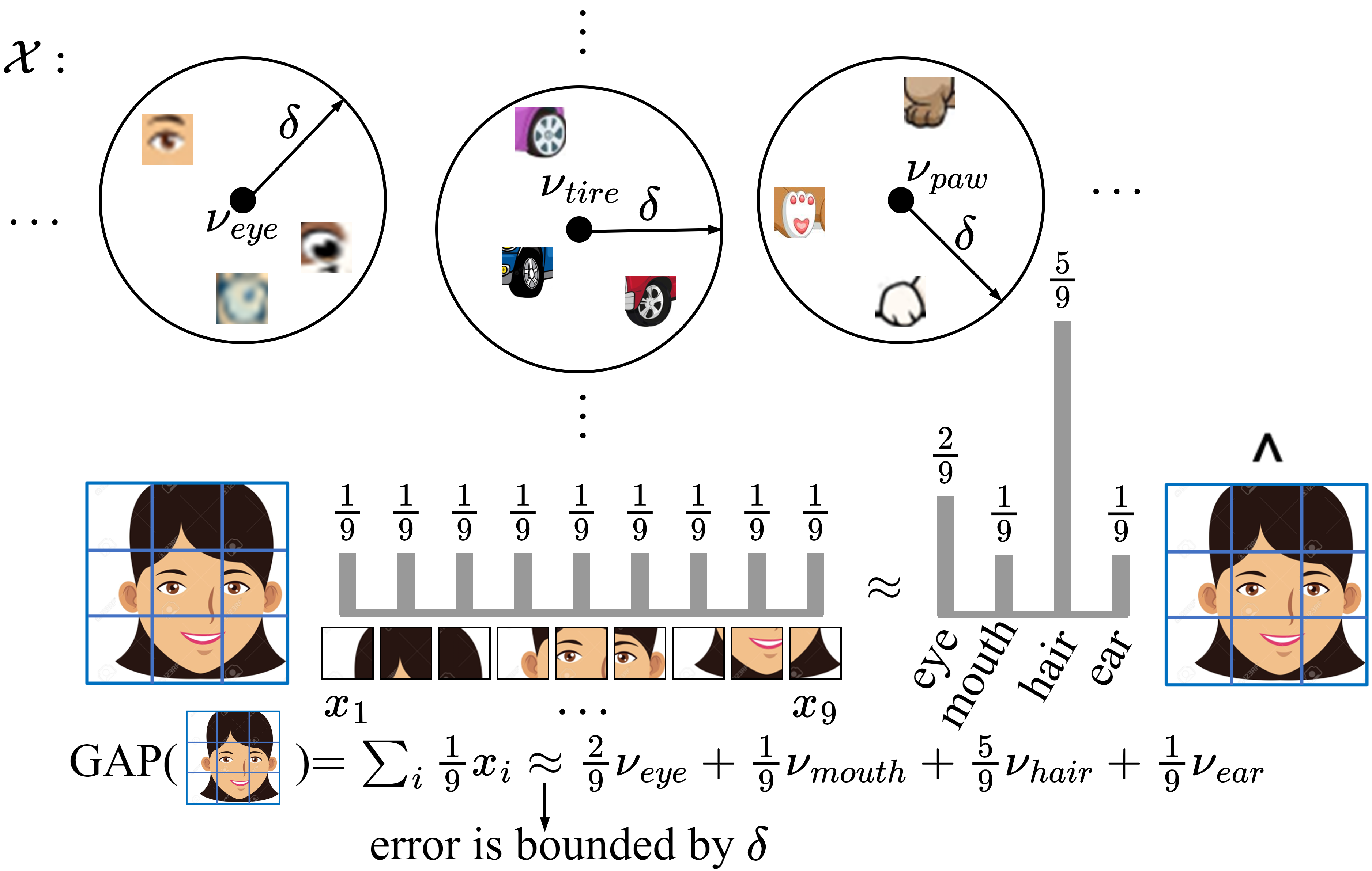
Though simple, GAP is a highly effective way to aggregate information. Empirically validated folklore [18, and references therein] to explain the effectiveness of GAP is considering each pixel of the CNN feature map as corresponding to a separate semantic entity and GAP as the combination of them [19]. A critical desiderata of DML is generalizing the learned embedding function to unseen classes. Thus, the learned semantic entities should be able to express novel classes, e.g., learning "tire" and "window" to represent "car" instead of learning "car". However, no explicit mechanism exists in the current DML approaches to enforce this behavior. Moreover, supervised DML losses provide guidance for seen classes, that yields entities fitted to classes and possibly hinders generalization capability. In this paper, we address explicitly learning generalizable semantic entities in the context of GAP.

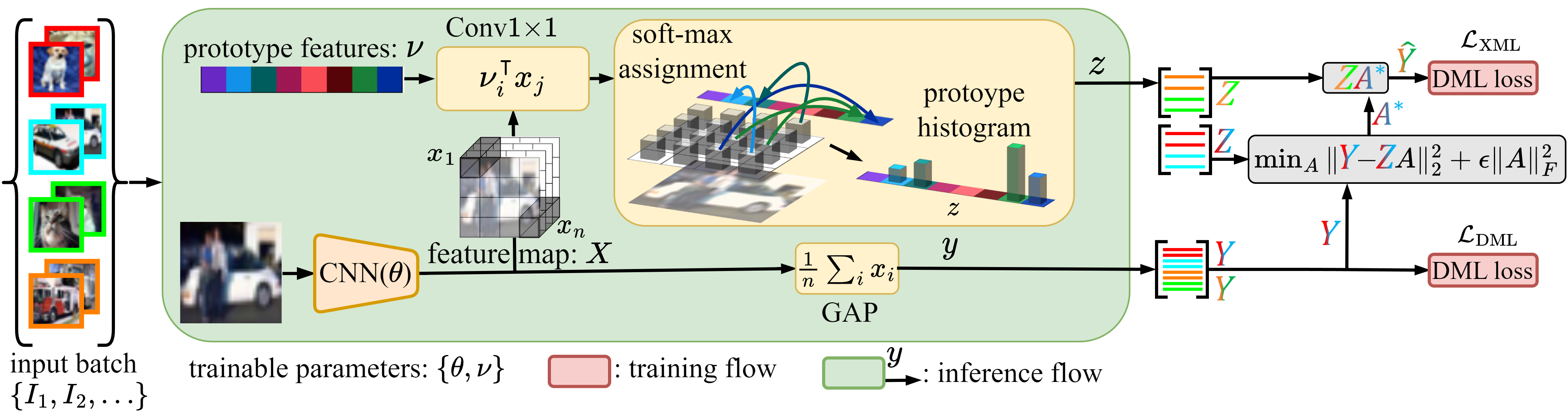
Briefly, our contributions include the following; $i)$ we formulate GAP as a convex combination of learnable prototypes (Fig.ย 1) to enable explicit learning of the semantic entities, $ii)$ we show that the prototype learning can be expressed as a recursive process fitting a linear predictor to the batch of samples, and $iii)$ we tailor a regularization loss (Fig.ย 2) built on expressing the set of classes with the prototypes fitted to another set of classes. Through rigorous experimentation, we validate our theoretical claims and demonstrate the effectiveness of our approach.

Refer to caption

Fig.ย 2: Embodiment of the method, where the histograms $Z{=}[z_{i}]_{i}$ (2.4) and GAP vectors $Y{=}[y_{i}]_{i}$ are coloured w.r.t. their class label.

2 Method

We propose a regularization loss to learn transferable features. Our loss is built on solving a metric learning problem on a batch and then evaluate the learned metric on another batch of unseen classes. We first express GAP as a convex combination of learnable prototypes in ยงย 2.1. We then associate prototype learning with a recursive process fitting a linear predictor to a batch of samples in ยงย 2.2. Building on that, we formulate our loss in ยงย 2.3. We defer all the upcoming proofs to appendix.

2.1 GAP as Convex Combination of Prototypes

We consider embedding functions that are implemented as CNN followed by GAP, i.e., $I\overset{\text{CNN}}{\longrightarrow}X\overset{\nicefrac{{1}}{{n}}\Sigma_{i}x_{i}}{\longrightarrow}y$ where $X$ is $w{\mathsf{x}}h$ feature map and $n=w{\mathsf{x}}h$. We introduce the following operator to compose a histogram representation from the collection of features.

Definition 2.1 (Histogram Operator)

For $n$-many $d$-dimensional features $X{=}[x_{i}{\in}\mathbb{R}^{d}]_{i=1}^{n}$ and $m$-many prototype features $\mathcal{V}=[\nu_{i}{\in}\mathbb{R}^{d}]_{i=1}^{m}$ of the same dimension, the histogram of $X$ on $\mathcal{V}$ is denoted as $z^{\ast}$ which is computed as the minimizer of the following problem:

$$(z^{\ast},\pi^{\ast})=\!\operatorname*{arg\,max}_{z\in\mathcal{S}^{m},\pi\geqslant 0}\!\textstyle\sum_{ij}\nu_{i}^{\intercal}x_{j}\pi_{ij}\text{ s.to }{\small\begin{array}[t]{l}\Sigma_{i}\pi_{ij}{=}\nicefrac{{1}}{{n}}\\[-3.87498pt] \Sigma_{j}\pi_{ij}{=}z_{i}\end{array}}$$ (2.1)

where $\mathcal{S}^{m}\coloneqq\{p\in\mathbb{R}^{m}_{\geqslant 0}\mid\Sigma_{i}p_{i}=1\}$.

Claim 2.1

The solution of the problem in (2.1) reads:

$$\pi^{\ast}_{ij}=\nicefrac{{1}}{{n}}\mathds{1}({i=\mathrm{argmax}_{k}\{\nu_{k}^{\intercal}x_{j}\}})$$ (2.2)

where $\mathds{1}(c)$ is 1 whenever $c$ is true and 0 otherwise.

In words, histogram operator basically assigns each feature to their nearest prototype and accumulates $\nicefrac{{1}}{{n}}$ mass for each assigned feature. We now consider a set of prototypes in the feature space $\mathcal{X}$ where the convolutional features $x_{i}$ lie. We consider $m$-many prototype features $\mathcal{V}=\{\nu_{i}\}_{i=1}^{m}$ so that the set $\mathcal{V}$ is $\delta$-cover of the feature space, $\mathcal{X}$. Namely, for any $x\in\mathcal{X}$, we have a prototype $\nu_{x}$ such that $\|x\shortminus\nu_{x}\|_{2}\leqslant\delta$.

Given $n$-many convolutional features $X=[x_{i}]_{i=1}^{n}$ we compute the histogram of $X$ on $\mathcal{V}$ (i.e., $z^{\ast}$) using (2.1) and obtain global representation $\hat{y}$ as:

$$\hat{y}=\textstyle\sum_{k=1}^{m}z^{\ast}_{k}\nu_{k}\quad.$$ (2.3)

Note that GAP representation is $y=\nicefrac{{1}}{{n}}\Sigma_{i=1}^{n}x_{i}$. By the following lemma, we show that GAP is approximately equivalent to $\hat{y}$, i.e., convex combination of prototypes.

Lemma 2.1

Given $n$-many convolutional features $X=[x_{i}{\in}\mathcal{X}]_{i=1}^{n}$ and $m$-many prototype features $\mathcal{V}=[\nu_{i}]_{i=1}^{m}$ with $\{\nu_{i}\}_{i=1}^{m}$ being $\delta$-cover of $\mathcal{X}$. If $z^{\ast}$ is the histogram of $X$ on $V$, defined in (2.1), then we have:

$$\|\textstyle\sum_{i=1}^{m}z^{\ast}_{i}\nu_{i}\shortminus\textstyle\sum_{j=1}^{n}\tfrac{1}{n}x_{j}\|_{2}\leqslant\delta$$

We visualize the result of Lemmaย 2.1 in Fig.ย 1, which implies that with GAP each image is represented as the convex combination of the prototype vectors. To generalize DML to unseen classes, we want the prototypes to represent transferable entities such as "tire" and "window" rather than classes themselves (e.g., "car"). To enforce that, we first formulate histogram operator as a trainable layer by smoothing the objective of (2.1) with entropy:

$$(z^{\prime},\pi^{\prime})=\!\operatorname*{arg\,max}_{\begin{subarray}{c}\Sigma_{i}\pi_{ij}{=}\nicefrac{{1}}{{n}}\\ \Sigma_{j}\pi_{ij}{=}z_{i}\\ z\in\mathcal{S}^{m},\pi>0\end{subarray}}\!\textstyle\sum_{ij}\nu_{i}^{\intercal}x_{j}\pi_{ij}-\tfrac{1}{\varepsilon}\textstyle\sum_{ij}\pi_{ij}\log\pi_{ij}$$ (2.4)

which admits soft-max solution as: $z^{\prime}_{i}=\tfrac{1}{n}\Sigma_{j}\tfrac{\mathrm{exp}(\varepsilon\nu_{i}^{\intercal}x_{j})}{\Sigma_{k}\mathrm{exp(\varepsilon\nu_{k}^{\intercal}x_{j})}}$. Thus, it can be implemented with $1{\mathsf{x}}1$ convolution and soft-max layers (Fig.ย 2). In the following sections, we derive a loss to regularize the learning of the prototypes.

2.2 Learning the Prototypes

Given $Z{=}[z_{i}]_{i}$ and $Y{=}[y_{i}]_{i}$ denoting the histograms obtained by (2.4) and GAP representations of a batch, respectively, we can learn the prototypes jointly with the embedding function by augmenting $\|\mathcal{V}Z\shortminus Y\|_{F}^{2}$ to the DML loss. However, that does not guarantee transferable representations. We now alternatively express the learning mechanism of the prototypes as a recursive process and derive a loss to regularize the learning.

Let $(Z_{1},Y_{1}),(Z_{2},Y_{2}),\ldots,(Z_{K},Y_{K})$ be the representations we obtain during the course of $K$-step training. We can obtain $\mathcal{V}^{(K)}$, i.e., the prototypes at $K$, as the solution of the following problem:

$$\mathcal{V}^{(K)}=\operatorname*{arg\,min}_{A}\textstyle\sum_{i=1}^{K}\alpha^{K-i}\|A\,Z_{i}-Y_{i}\|_{F}^{2}+\beta\|A\|_{F}^{2}$$ (2.5)

where $0<\alpha\leqslant 1$ is the forgetting factor to put more emphasis on the recent representations, and $\beta\|A\|_{F}^{2}$ is to improve robustness. We can obtain the solution as [20]:

$$\mathcal{V}^{(K)}=R_{K}^{\shortminus 1}Q_{K}$$ (2.6)

where $R_{K}=\Sigma_{i}\alpha^{K-i}Z_{i}Z_{i}^{\intercal}+\beta I$ and $Q_{K}=\Sigma_{i}\alpha^{K-i}Z_{i}Y_{i}^{\intercal}$. For a new batch $(Z,Y)$ at step $K+1$, we can update the solution as:

$$\mathcal{V}^{(K+1)}=W_{K}\mathcal{V}^{(K)}+(I-W_{K})\mathcal{V}$$ (2.7)

where $\mathcal{V}=\operatorname*{arg\,min}_{A}\|A\,Z-Y\|^{2}_{F}+(1\shortminus\alpha)\beta\|A\|_{F}^{2}$ is the prototypes fitted to the current batch as $\mathcal{V}=R^{\shortminus 1}Z\,Y^{\intercal}$ with $R^{\shortminus 1}=Z\,Z^{\intercal}+(1\shortminus\alpha)\beta I$, and $W_{K}=R^{\shortminus 1}(R_{K}^{\shortminus 1}+\alpha R^{\shortminus 1})^{\shortminus 1}$. The results mainly come from Woodbury identity similar to derivation of RLS filter [20].

Practically, learning prototypes with gradient descent of $\|\mathcal{V}Z\shortminus Y\|_{F}^{2}$ is more appealing. That said, the form of the recursive update in (2.7) reveals that the learned prototypes are the weighted combinations of the prototypes fitted to the batch of samples. Thus, imposing constraints on per-batch-fitted prototypes can be a decisive step to obtain a batch-based regularization loss. In the following section, we build on that perspective to formulate our loss to regularize prototype learning.

2.3 Cross-batch Metric Learning

The formulation in (2.7) reinterprets the learning mechanism of prototypes, that is based on iteratively fitting prototypes to batch of samples $(Z,Y)$ as:

$$\mathcal{V}=\operatorname*{arg\,min}_{A}\|A\,Z-Y\|_{F}^{2}+\epsilon\|A\|_{F}^{2}$$ (2.8)

Assuming that representations in $Y$ are consistent with the label information, expression in (2.8) is equivalent to solving a metric learning problem for $(Z,Y)$ tuples [21]. We now exploit this observation to derive our loss.

We first split the batch $(Z,Y)$ into two as $(Z_{1},Y_{1})$ and $(Z_{2},Y_{2})$ such that class sets of the two batches are disjoint. Similar to (2.7), we express (2.8) as:

$$\mathcal{V}=W\mathcal{V}_{1}+(I-W)\mathcal{V}_{2}$$ (2.9)

where $\mathcal{V}_{k}=\operatorname*{arg\,min}_{A}\|A\,Z_{k}-Y_{k}\|_{F}^{2}+\nicefrac{{\epsilon}}{{2}}\|A\|_{F}^{2}$, and $W=R_{2}^{\shortminus 1}(R_{1}^{\shortminus 1}+R_{1}^{\shortminus 2})^{\shortminus 1}$ with $R_{k}=Z_{k}\,Z_{k}^{T}+\nicefrac{{\epsilon}}{{2}}I$. Hence, we express the learning mechanism at each batch as the weighted combination of the two metrics fitted to the different sets of classes, that sets the stage for the rest of the formulation.

Consider the prototypes $\mathcal{V}_{1}$ fitted to $(Z_{1},Y_{1})$. If those prototypes, $\mathcal{V}_{1}$, are corresponding to transferable entities, then their combination with the weights in $Z_{2}$ should yield embeddings that are consistent with the label information. Specifically, $\hat{Y}_{2}=\mathcal{V}_{1}\,Z_{2}$ should also minimize DML loss.

Formally, given a batch $(Z{=}[Z_{1}\,Z_{2}],Y{=}[Y_{1}\,Y_{2}])$, we first obtain the prototypes as $\mathcal{V}_{k}=(Z_{k}\,Z_{k}^{\intercal}+\epsilon I)^{\shortminus 1}Z_{k}\,Y_{k}^{\intercal}$ for $k{\in}\{1,2\}$ or equivalently $\mathcal{V}_{k}=Y_{k}(Z_{k}^{\intercal}Z_{k}+\epsilon I)^{\shortminus 1}Z_{k}^{\intercal}$, if the batch size is less than the number of prototypes for computational efficiency. Given a DML loss function $\ell((y_{i},L_{i}),(y_{j},L_{j}))$, e.g., contrastive [1], we formulate our cross-batch metric learning (XML) loss as:

$$\mathcal{L}_{\text{XML}}=\textstyle\sum\limits_{k}\textstyle\sum\limits_{\hat{y}_{i},\hat{y}_{j}\in\hat{Y}_{k}}\ell((\hat{y}_{i},L_{i}),(\hat{y}_{j},L_{j}))$$ (2.10)

for $k{=}1,2$ where $\hat{Y}_{1}=\mathcal{V}_{2}\,Z_{1}$ and $\hat{Y}_{2}=\mathcal{V}_{1}\,Z_{2}$. In words, we solve a metric learning problem for a set of classes and then compute its performance on another set of unseen classes. Having closed form solution for $\mathcal{V}_{k}$ in terms of $(Z_{k},Y_{k})$ enables us to express the metric learning problem as a differentiable operation. Hence, unseen class performance can be explicitly enforced through a batch-based loss term (i.e., $\mathcal{L}_{\text{XML}}$) that can be jointly optimized with gradient descent of any DML loss. In particular, we combine this loss with the metric learning loss as:

$$\mathcal{L}=(1{\shortminus}\lambda)\mathcal{L}_{\text{DML}}+\lambda\mathcal{L}_{\text{XML}}$$ (2.11)

The proposed loss assesses the unseen class generalization performance of locally fitted prototypes. Intuitively, such a regularization in learning should be useful in better generalization of the CNN features as well as GAP embeddings since prototypes are connected to CNN features and GAP embeddings through analytical operations.

3 Experimental Work

We start our empirical study with evaluations on DML benchmarks to show the effectiveness of XML. We extend our study further to validate the role of XML in learning.

3.1 Deep Metric Learning Experiments

Table 1: Evaluation on 4 DML benchmarks with 2 widely-acknowledged settings. Red: the best. Blue: the second best. Bold: improvement over baseline.
Dataset$\rightarrow$ SOP InShop CUB Cars
Setting$\rightarrow$ BNInception - MLRC Evaluation (MAP@R)
Method$\downarrow$ 512D 128D 512D 128D 512D 128D 512D 128D
Triplet[2] 45.88 40.01 59.67 54.25 23.65 18.54 22.67 15.74
MS[3] 44.19 40.34 58.79 54.85 24.95 20.13 27.16 18.73
PNCA++[8] 47.11 43.57 57.58 54.41 25.27 20.63 26.21 18.61
Contrastive[1] 45.85 41.79 59.07 55.38 25.95 20.58 24.38 17.02
C+XML 46.84 42.73 59.75 55.63 27.58 22.03 26.33 18.31
PAnchor[7] 48.08 44.33 58.02 54.98 26.20 20.94 27.14 19.15
PA+XML 49.16 45.15 58.66 55.46 26.51 21.34 27.56 19.28
Setting$\rightarrow$ ResNet50 - Conventional Evaluation (R@1)
PAnchor[7] 80.00 92.10 69.70 87.70
MS+Metrix[6] 81.00 92.20 71.40 89.60
LIBC[11] 81.40 92.80 70.30 88.10
LIBC+XML 81.48 93.04 70.49 88.38

Setup. We evaluate our method on CUB [22], Cars [23], InShop [24], and SOP [25]. Minimizing the confounding of factors other than our proposed method, we keep the comparisons as fair as possible following the MLRC [4] procedures with BNInception embeddings [26]. We additionally evaluate XML following the conventional settings [11] with ResNet50 [27] embeddings. For XML, $\varepsilon{=}10$, $\lambda{=}0.01$, $\epsilon{=}0.05$, and $m{=}64$ in CUB&Cars, and $m{=}128$ in SOP&InShop, based on our empirical analysis.

Results. We apply XML with contrastive [1] (C+ XML) and ProxyAnchor [7] (PA+XML) losses in MLRC setting, and with LIBC [11] in conventional setting. For MLRC, we report average (128D) and concatenated (512D) model MAP@R [4] performance, and R@1 for the conventional evaluation in Tab.ย 1 (higher the better). We observe consistent improvements upon direct application of DML losses in all datasets and boost state-of-the-art.

3.2 Proof of the Concept

For the following, we perform DML trainings with XML on Cifar10 [28] dataset using ResNet20 [27] architecture.

Refer to caption


Fig.ย 3: Prototypes with their covering radius (left), and GAP and PCC embedding of a sample (right) with the assigned prototypes.

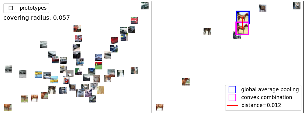
GAP and prototypes. To empirically verify Lemmaย 2.1, we use 2D feature embeddings for direct visualization. We sample 64 images from each class and obtain the local CNN features as well as the GAP features. We compute $48$-many prototypes among the local features using greedy k-center [9]. We plot the prototypes in Fig.ย 3 where we see that prototypes correspond to generalizable semantic entities. We also provide the covering radius (i.e., $\delta$ in $\delta$-cover) of the prototype set and the discrepancy between GAP and prototype convex combination (PCC) embeddings, which is less than $\delta$ as Lemmaย 2.1 claims.

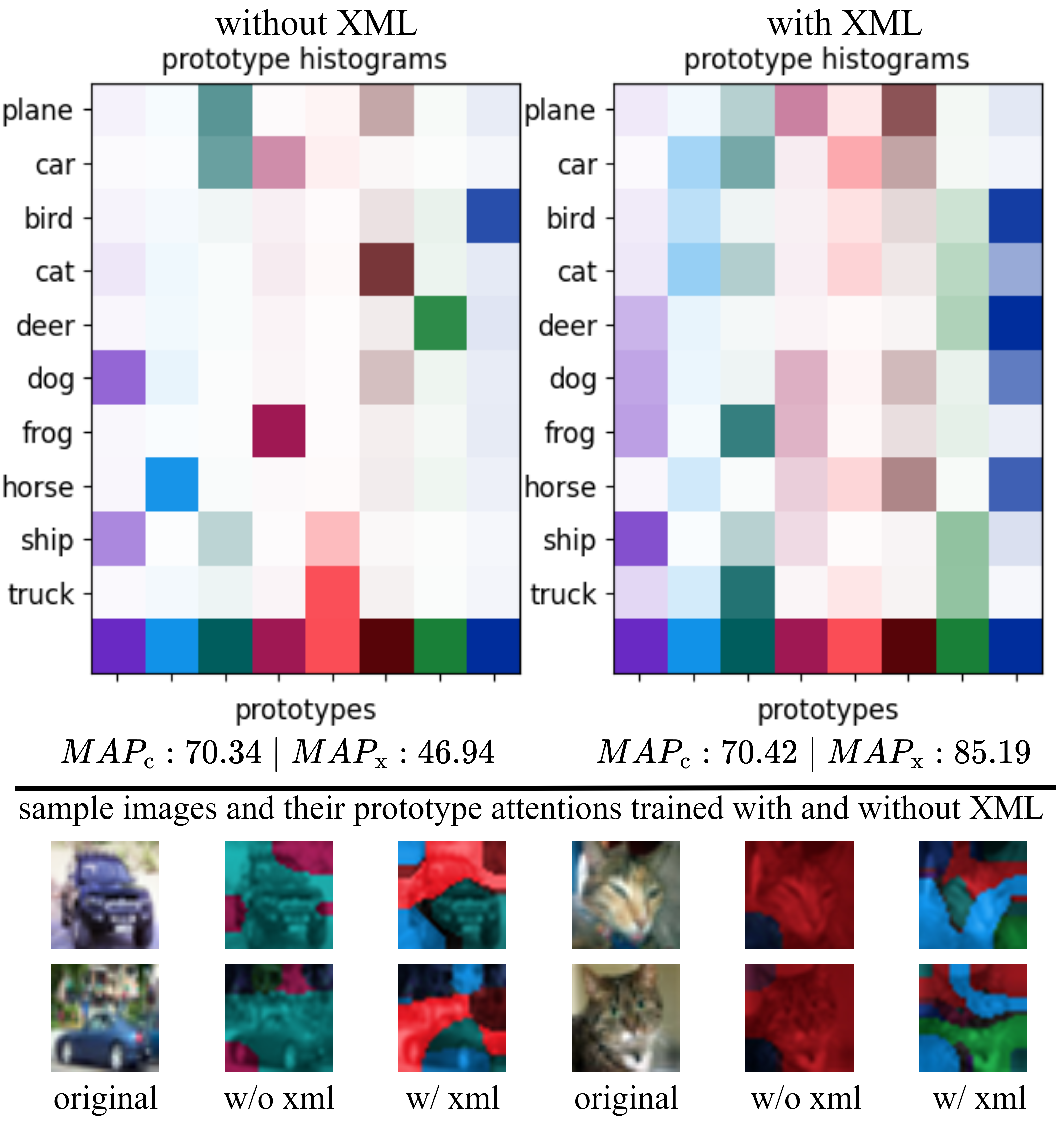
Prototypes with XML. We test the impact of XML on learned prototypes by performing DML on Cifar10 with 8 prototypes. We compare results with and without $\mathcal{L}_{\text{XML}}$ and visualize the prototype histograms for each class in Fig.ย 4. With $\mathcal{L}_{\text{XML}}$, we observe transferable representations and that the prototypes are fit to transferable entities while they are fit to classes without it. For instance, XML prototypes represent a "car" in terms of parts and use some of them in the representation of "cat" as well. We quantitatively evaluate this behavior by randomly splitting the classes in half and using cross-batch metric learning in ยงย 2.3. Our evaluation shows that the features and prototypes with XML have superior unseen class generalization ($MAP_{x}$) while the seen class performances ($MAP_{c}$) are similar. We repeated the experiment 1000 times to ensure validity.

Refer to caption


Fig.ย 4: The distributions of the learned 8 prototypes across classes of Cifar10 dataset with and without $\mathcal{L}_{\text{XML}}$. Attention maps are coloured according to the dominant prototype at that location. $MAP_{c}$ denotes the performance of metric learning fitted to all classes and $MAP_{x}$ denotes the cross-class performance, i.e. metric learning fitted to 5 classes and evaluated on the other 5 classes.

4 Conclusion

Building on the perspective explaining GAP as the convex combination of prototypes, we formulated learning of the prototypes and proposed cross-batch metric learning loss to regularize the learning for transferable prototypes. With extensive empirical studies, we validated the effectiveness of our method in various DML benchmarks.

References

  • [1] C.-Y.Wu, R.Manmatha, A.ย J.Smola, and P.Krahenbuhl, โ€œSampling matters in deep embedding learning,โ€ in ICCV, 2017.
  • [2] F.Schroff, D.Kalenichenko, and J.Philbin, โ€œFacenet: A unified embedding for face recognition and clustering,โ€ in CVPR, 2015.
  • [3] X.Wang, X.Han, W.Huang, D.Dong, and M.ย R.Scott, โ€œMulti-similarity loss with general pair weighting for deep metric learning,โ€ in CVPR, 2019.
  • [4] K.Musgrave, S.Belongie, and S.-N.Lim, โ€œA metric learning reality check,โ€ in ECCV, 2020.
  • [5] K.Roth, T.Milbich, S.Sinha, P.Gupta, B.Ommer, and J.ย P.Cohen, โ€œRevisiting training strategies and generalization performance in deep metric learning,โ€ in ICML, 2020.
  • [6] S.Venkataramanan, B.Psomas, E.Kijak, laurent amsaleg, K.Karantzalos, and Y.Avrithis, โ€œIt takes two to tango: Mixup for deep metric learning,โ€ in ICLR, 2022.
  • [7] S.Kim, D.Kim, M.Cho, and S.Kwak, โ€œProxy anchor loss for deep metric learning,โ€ in CVPR, 2020.
  • [8] E.ย W.Teh, T.DeVries, and G.ย W.Taylor, โ€œProxynca++: Revisiting and revitalizing proxy neighborhood component analysis,โ€ in ECCV, 2020.
  • [9] Y.ย Z.Gurbuz, O.Can, and A.ย A.Alatan, โ€œDeep metric learning with chance constraints,โ€ arXiv preprint arXiv:2209.09060, 2022.
  • [10] K.Roth, B.Brattoli, and B.Ommer, โ€œMic: Mining interclass characteristics for improved metric learning,โ€ in ICCV, 2019.
  • [11] J.Seidenschwarz, I.Elezi, and L.Leal-Taixรฉ, โ€œLearning intra-batch connections for deep metric learning,โ€ in ICML, 2021.
  • [12] O.Can, Y.ย Z.Gรผrbรผz, and A.ย A.Alatan, โ€œDeep metric learning with alternating projections onto feasible sets,โ€ in ICIP, 2021.
  • [13] Y.Patel, G.Tolias, and J.Matas, โ€œRecall@ k surrogate loss with large batches and similarity mixup,โ€ in CVPR, 2022.
  • [14] K.Roth, O.Vinyals, and Z.Akata, โ€œNon-isotropy regularization for proxy-based deep metric learning,โ€ in CVPR, 2022.
  • [15] W.Zheng, B.Zhang, J.Lu, and J.Zhou, โ€œDeep relational metric learning,โ€ in ICCV, 2021.
  • [16] T.Milbich, K.Roth, H.Bharadhwaj, S.Sinha, Y.Bengio, B.Ommer, and J.ย P.Cohen, โ€œDiva: Diverse visual feature aggregation for deep metric learning,โ€ in ECCV, 2020.
  • [17] K.Roth, T.Milbich, B.Ommer, J.ย P.Cohen, and M.Ghassemi, โ€œS2sd: Simultaneous similarity-based self-distillation for deep metric learning,โ€ in ICML, 2021.
  • [18] B.Zhou, D.Bau, A.Oliva, and A.Torralba, โ€œInterpreting deep visual representations via network dissection,โ€ TPAMI, 2018.
  • [19] Y.ย Z.Gรผrbรผz and A.ย A.Alatan, โ€œA novel bovw mimicking end-to-end trainable cnn classification framework using optimal transport theory,โ€ in ICIP, 2019.
  • [20] M.ย H.Hayes, Statistical digital signal processing and modeling, John Wiley & Sons, 1996.
  • [21] M.Perrot and A.Habrard, โ€œRegressive virtual metric learning,โ€ in Advances in Neural Information Processing Systems, 2015, pp. 1810โ€“1818.
  • [22] C.Wah, S.Branson, P.Welinder, P.Perona, and S.Belongie, โ€œThe caltech-ucsd birds-200-2011 dataset,โ€ 2011.
  • [23] A.Krause and D.Golovin, โ€œSubmodular function maximization,โ€ in Tractability: Practical Approaches to Hard Problems, pp. 71โ€“104. Cambridge University Press, 2014.
  • [24] Z.Liu, P.Luo, S.Qiu, X.Wang, and X.Tang, โ€œDeepfashion: Powering robust clothes recognition and retrieval with rich annotations,โ€ in CVPR, 2016.
  • [25] H.Ohย Song, Y.Xiang, S.Jegelka, and S.Savarese, โ€œDeep metric learning via lifted structured feature embedding,โ€ in CVPR, 2016.
  • [26] S.Ioffe and C.Szegedy, โ€œBatch normalization: Accelerating deep network training by reducing internal covariate shift,โ€ in ICML, 2015.
  • [27] K.He, X.Zhang, S.Ren, and J.Sun, โ€œIdentity mappings in deep residual networks,โ€ in ECCV, 2016.
  • [28] A.Krizhevsky and G.Hinton, โ€œLearning multiple layers of features from tiny images,โ€ Tech. Rep., Citeseer, 2009.
  • [29] B.ย K.Sriperumbudur, A.Gretton, K.Fukumizu, B.Schรถlkopf, and G.ย R.Lanckriet, โ€œHilbert space embeddings and metrics on probability measures,โ€ The Journal of Machine Learning Research, vol. 11, pp. 1517โ€“1561, 2010.

Appendix

Preliminaries

Definition 1 (Optimal Transport Distance)

The optimal transport (OT) distance between two probability mass distributions $(p,X)$ and $(q,Y)$ is:

$$\|(p,X)\shortminus(q,Y)\|_{OT}=\!\!\!\min_{\begin{subarray}{c}\pi\geqslant 0\\ \Sigma_{i}\pi_{ij}=q_{j}\\ \Sigma_{j}\pi_{ij}=p_{i}\end{subarray}}\!\!\textstyle\sum_{ij}c_{ij}\pi_{ij}$$ (A.1)

where $c_{ij}=\|x_{i}\shortminus y_{j}\|_{2}$, and $(p,X)\in\Sigma_{n}\times\mathbb{R}^{d\times n}$ denotes a probability mass distribution with masses $p\in\Sigma_{n}$ in the probability simplex (i.e., $\Sigma_{n}\coloneqq\{p\in\mathbb{R}^{n}_{\geqslant 0}\mid\textstyle\sum_{i}p_{i}=1\}$), and $d$-dimensional support $X=[x_{i}]_{i\in[n]}\in\mathbb{R}^{d\mathsf{x}n}$.

Definition 2 (Maximum Mean Discrepancy)

Max-imum mean discrepancy (MMD) between two probability mass distributions $(p,X)$ and $(q,Y)$ is:

$$\|(p,X)\shortminus(q,Y)\|_{MMD}=\!\!\max_{f\in\mathcal{C}(X,Y)}\textstyle\sum_{i}p_{i}f(x_{i})-\textstyle\sum_{j}q_{j}f(y_{j})$$ (A.2)

where $\mathcal{C}(X,Y)$ is the set of continuous and bounded functions defined on a set covering the column vectors of $X$ and $Y$.

Definition 3 (Optimal Transport Distance Dual)

The Lagrangian dual of the optimal transport distance defined in 1 reads:

$$\|(p,X)\shortminus(q,Y)\|_{OT}=\!\!\!\max_{f_{i}+g_{j}\leqslant c_{ij}}\!\!\textstyle\sum_{i}p_{i}f_{i}+\textstyle\sum_{j}q_{j}g_{j}$$ (A.3)

with the dual variables $\lambda=\{f,g\}$.

Note that $x_{i}=y_{j}$ implies $f_{i}=-g_{j}$ and from the fact that $c_{ij}=c_{ji}$, we can express the problem in (A.3) as:

$$\|(p,X)\shortminus(q,Y)\|_{OT}=\max_{f\in\mathfrak{L}_{1}}\textstyle\sum_{i}p_{i}f(x_{i})-\textstyle\sum_{j}q_{j}f(x_{j})$$ (A.4)

where $\mathfrak{L}_{1}=\{f\mid\sup\limits_{x,y}\tfrac{|f(x)-f(y)|}{\|x-y\|_{2}}\leqslant 1\}$ is the set of 1-Lipschitz functions.

Proofs

Definition 4 (Histogram Operator)

For $n$-many $d$-dimensional features $X{=}[x_{i}{\in}\mathbb{R}^{d}]_{i=1}^{n}$ and $m$-many prototype features $\mathcal{V}=[\nu_{i}{\in}\mathbb{R}^{d}]_{i=1}^{m}$ of the same dimension, the histogram of $X$ on $\mathcal{V}$ is denoted as $z^{\ast}$ which is computed as the minimizer of the following problem:

$$(z^{\ast},\pi^{\ast})=\!\operatorname*{arg\,max}_{z\in\mathcal{S}^{m},\pi\geqslant 0}\!\textstyle\sum_{ij}\nu_{i}^{\intercal}x_{j}\pi_{ij}\text{ s.to }{\small\begin{array}[t]{l}\Sigma_{i}\pi_{ij}{=}\nicefrac{{1}}{{n}}\\[-3.87498pt] \Sigma_{j}\pi_{ij}{=}z_{i}\end{array}}$$ (A.5)

where $\mathcal{S}^{m}\coloneqq\{p\in\mathbb{R}^{m}_{\geqslant 0}\mid\Sigma_{i}p_{i}=1\}$.

Claim 1

The solution of the problem in (A.5) reads:

$$\pi^{\ast}_{ij}=\nicefrac{{1}}{{n}}\mathds{1}({i=\mathrm{argmax}_{k}\{\nu_{k}^{\intercal}x_{j}\}})$$ (A.6)

where $\mathds{1}(c)$ is 1 whenever $c$ is true and 0 otherwise.

Proof: We prove our claim by contradiction. Denoting $c_{ij}=-\nu_{i}^{\intercal}x_{j}$, for any $j$, we express a solution as $\pi^{\ast}_{ij}=\epsilon_{i}$ with $\epsilon_{i}\geqslant 0$ and $\sum_{i}\epsilon_{i}=\nicefrac{{1}}{{n}}$. Let $i^{\ast}=\operatorname*{arg\,min}_{k}\{c_{kj}\}$. We can write ฯ€iโˆ—โ€‹jโˆ—=1/nโˆ’โˆ‘iโˆฃiโ‰ iโˆ—ฯตisubscriptsuperscript๐œ‹โˆ—superscript๐‘–โˆ—๐‘—1๐‘›subscriptconditional๐‘–๐‘–superscript๐‘–โˆ—subscriptitalic-ฯต๐‘–\pi^{\ast}_{i^{\ast}j}=\nicefrac{{1}}{{n}}-\sum_{i\mid i\neq i^{\ast}}\epsilon_{i}. Our claim states that $\epsilon_{i}=0$ for iโ‰ iโˆ—๐‘–superscript๐‘–โˆ—i\neq i^{\ast}. We assume an optimal solution, $\pi^{\prime}$, with $\epsilon_{i}>0$ for some iโ‰ iโˆ—๐‘–superscript๐‘–โˆ—i\neq i^{\ast}. Since $\pi^{\prime}$ is optimal, we must have $\sum_{ij}\pi^{\prime}_{ij}c_{ij}\leqslant\sum_{ij}\pi_{ij}c_{ij}$ for any $\pi$. For the $j^{th}$ column we have,

โˆ‘iฯ€iโ€‹jโ€ฒโ€‹ciโ€‹j=(1nโˆ’โˆ‘iโ€ฒโˆฃiโ€ฒโ‰ iโˆ—ฯตiโ€ฒ)โ€‹ciโˆ—โ€‹j+โˆ‘iโ€ฒโˆฃiโ€ฒโ‰ iโˆ—ฯตiโ€ฒโ€‹ciโ€ฒโ€‹j=1nโ€‹ciโˆ—โ€‹j+โˆ‘iโ€ฒโˆฃiโ€ฒโ‰ iโˆ—ฯตiโ€ฒโ€‹(ciโ€ฒโ€‹jโˆ’ciโˆ—โ€‹j)โ€‹>(a)โ€‹โˆ‘iฯ€iโ€‹jโˆ—โ€‹ciโ€‹jsubscript๐‘–subscriptsuperscript๐œ‹โ€ฒ๐‘–๐‘—subscript๐‘๐‘–๐‘—1๐‘›subscriptconditionalsuperscript๐‘–โ€ฒsuperscript๐‘–โ€ฒsuperscript๐‘–โˆ—subscriptitalic-ฯตsuperscript๐‘–โ€ฒsubscript๐‘superscript๐‘–โˆ—๐‘—subscriptconditionalsuperscript๐‘–โ€ฒsuperscript๐‘–โ€ฒsuperscript๐‘–โˆ—subscriptitalic-ฯตsuperscript๐‘–โ€ฒsubscript๐‘superscript๐‘–โ€ฒ๐‘—1๐‘›subscript๐‘superscript๐‘–โˆ—๐‘—subscriptconditionalsuperscript๐‘–โ€ฒsuperscript๐‘–โ€ฒsuperscript๐‘–โˆ—subscriptitalic-ฯตsuperscript๐‘–โ€ฒsubscript๐‘superscript๐‘–โ€ฒ๐‘—subscript๐‘superscript๐‘–โˆ—๐‘—๐‘Žsubscript๐‘–subscriptsuperscript๐œ‹โˆ—๐‘–๐‘—subscript๐‘๐‘–๐‘—\begin{split}\textstyle\sum_{i}\pi^{\prime}_{ij}c_{ij}&=(\tfrac{1}{n}-\textstyle\sum\limits_{i^{\prime}\mid i^{\prime}\neq i^{\ast}}\epsilon_{i^{\prime}})c_{i^{\ast}j}+\textstyle\sum\limits_{i^{\prime}\mid i^{\prime}\neq i^{\ast}}\epsilon_{i^{\prime}}c_{i^{\prime}j}\\ &=\tfrac{1}{n}c_{i^{\ast}j}+\textstyle\sum\limits_{i^{\prime}\mid i^{\prime}\neq i^{\ast}}\epsilon_{i^{\prime}}(c_{i^{\prime}j}-c_{i^{\ast}j})\overset{(a)}{>}\textstyle\sum_{i}\pi^{\ast}_{ij}c_{ij}\end{split}

where in $(a)$ we use the fact that $(c_{i^{\prime}j}-c_{i^{\ast}j})>0$ and $\epsilon_{i^{\prime}}>0$ for some $i^{\prime}$ by the assumption. Hence, $\textstyle\sum_{ij}\pi^{\prime}_{ij}c_{ij}>\textstyle\sum_{ij}\pi^{\ast}_{ij}c_{ij}$ poses a contradiction. Therefore, $\epsilon_{i^{\prime}}=0$ must hold for all iโ€ฒโ‰ iโˆ—superscript๐‘–โ€ฒsuperscript๐‘–โˆ—i^{\prime}\neq i^{\ast}. โ– โ– \blacksquare

Lemma 1

Given $n$-many convolutional features $X=[x_{i}{\in}\mathcal{X}]_{i=1}^{n}$, and $m$-many prototype features $\mathcal{V}=[\nu_{i}]_{i=1}^{m}$ with $\{\nu_{i}\}_{i=1}^{m}$ being $\delta$-cover of $\mathcal{X}$. If $z^{\ast}$ is the histogram of $X$ on $V$, defined in (A.5), then we have:

$$\|\textstyle\sum_{i=1}^{m}z^{\ast}_{i}\nu_{i}\shortminus\textstyle\sum_{j=1}^{n}\tfrac{1}{n}x_{j}\|_{2}\leqslant\delta$$

Proof: We can express

$$\|\textstyle\sum\limits_{i\in[m]}z^{\ast}_{i}\nu_{i}\shortminus\textstyle\sum\limits_{j\in[n]}\tfrac{1}{n}x_{j}\|_{2}^{2}=\textstyle\sum\limits_{i\in[m]}p^{\ast}_{i}f(\nu_{i})\shortminus\textstyle\sum\limits_{j\in[n]}q_{j}f(x_{j})$$

where $f(x)=x^{\intercal}(\textstyle\sum_{i}z^{\ast}_{i}\nu_{i}\shortminus\textstyle\sum_{j}\tfrac{1}{n}x_{j})$, and $[n]=1,\ldots,n$. Note that $f$ is a continuous bounded operator for $\mathcal{X}=\{x\mid\|x\|_{2}\leqslant 1\}$ (We can always map the features inside unit sphere without loosing the relative distances). Moreover, the operator norm of $f$, i.e. $\|f\|$, which is $\|\textstyle\sum_{i}z^{\ast}_{i}\nu_{i}\shortminus\textstyle\sum_{j}\tfrac{1}{n}x_{j}\|_{2}$ is less than or equal to 1. Thus, $f$ lie in the unit sphere of the continuous bounded functions set. Using the definition of MMD distance, we can bound the error as:

$$\textstyle\sum\limits_{i\in[m]}z^{\ast}_{i}f(\nu_{i})\shortminus\textstyle\sum\limits_{j\in[n]}q_{j}f(x_{j})\leqslant\|(z^{\ast},V)\shortminus(q,X)\|_{MMD}$$

where $q_{i}=\nicefrac{{1}}{{n}}$ for all $i$. For the continuous and bounded functions of the operator norm less than 1, MMD is lower bound for OT [29]. Namely,

$$\begin{split}\textstyle\sum\limits_{i\in[m]}z^{\ast}_{i}f(\nu_{i})\shortminus\textstyle\sum\limits_{j\in[n]}q_{j}f(x_{j})&\leqslant\|(z^{\ast},V)\shortminus(q,X)\|_{MMD}\\ &\leqslant\|(z^{\ast},V)\shortminus(q,X)\|_{OT}\end{split}$$

Since columns of $V$ is $\delta$-cover of the set $\mathcal{X}$, the optimal transport distance between the two distributions are bounded by $\delta$, i.e. $\|(z^{\ast},V)\shortminus(q,X)\|_{OT}\leqslant\delta$. Thus, we finally have:

$$\|\textstyle\sum\limits_{i\in[m]}z^{\ast}_{i}\nu_{i}\shortminus\textstyle\sum\limits_{j\in[n]}\tfrac{1}{n}x_{j}\|_{2}\leqslant\delta.$$

โ– โ– \blacksquare