Stochastic dynamics and the Polchinski equation: an introduction

Abstract

This introduction surveys a renormalisation group perspective on log-Sobolev inequalities and related properties of stochastic dynamics. We also explain the relationship of this approach to related recent and less recent developments such as Eldan’s stochastic localisation and the Föllmer process, the Boué–Dupuis variational formula and the Barashkov–Gubinelli approach, the transportation of measure perspective, and the classical analogues of these ideas for Hamilton–Jacobi equations which arise in mean-field limits.

1 Introduction

Functional inequalities have been thoroughly studied in different contexts [62, 7] and one important motivation is to quantify the relaxation of stochastic dynamics by using Poincaré and (possibly modified) log-Sobolev inequalities [68, 51, 86, 37, 22]. Statistical mechanics offers an interesting setting to apply these inequalities and to analyse the information they provide in various physical regimes. Indeed, one would like to describe the relaxation to equilibrium of lattice gas and spin dynamics, which are modelled by stochastic evolutions on high-dimensional state spaces. Their continuum limits, often described by (singular) SPDEs, are also of a lot of interest.

The structure of the equilibrium Gibbs measures is sensitive to the occurrence of phase transitions and the dynamical behaviour will also be strongly influenced by phase transitions. In the uniqueness regime, namely in absence of a phase transition (typically at high temperatures), one expects that the dynamics relax exponentially fast uniformly in the dimension of the state space with a speed of relaxation diverging when the temperature approaches the critical point. We refer to Sections 2.6 and 2.7 for more details. In a phase transition regime (typically corresponding to low temperatures), one expects different types of behaviours depending strongly on the type of boundary conditions and we will not discuss the corresponding phenomena in these notes.

The fast relaxation towards equilibrium in the uniqueness regime (or at least deep in it) is well understood and we refer to [68, 69, 51] for very complete accounts of the corresponding theory. Roughly speaking, it has been shown for a wide range of models that good mixing properties of the equilibrium measure are equivalent to fast relaxation of the dynamics, namely uniform bounds (with respect to the domains and the boundary conditions) on the Poincaré or the log-Sobolev constants. For the Ising model [68, 35, 38], the validity of the mixing properties have been proved in the whole uniqueness regime leading to strong relaxation statements on the dynamics, and more detailed dynamical features are also understood in that regime [67, 66]. For more general systems and in particular continuous spin systems, the picture is much less complete.

The main goal of this survey is to present a different perspective on the derivation of functional inequalities based on the renormalisation group theory, introduced in physics by Wilson [89], and with its continuous formulation emphasised in particular by Polchinski [78]. The renormalisation group was introduced to study the critical behaviour and the existence of continuum limits of equilibrium models of statistical physics and quantum field theory from a unified perspective. The renormalisation group formalism associates with a Gibbs measure a flow of measures defined in terms of a renormalised potential (see Section 3.2). We show how this structure can be used to prove log-Sobolev inequalities under a condition on the renormalised potential which is a multiscale generalisation of the Bakry-Émery criterion (see Section 3.3). The renormalised potential obeys a second-order Hamilton–Jacobi type equation (the Polchinski equation) with characteristics given by a stochastic evolution (see Section 4.1) which coincide with the stochastic process of Eldan’s stochastic localisation method introduced for very different purposes [40]. Section 4.5 provides a dictionary to relate both points of view.

An alternative to the multiscale Bakry–Émery method to derive log-Sobolev inequalities (with much similarity and both advantages and disadvantages) is the entropic stability estimate recently established in [28] and reviewed in Section 3.7. This estimate applies to the same Polchinki flow, or its equivalent interpretation as stochastic localisation. It originated in the spectral and entropic independence estimates [4, 3] which are similar estimates for a different flow that takes the role of the Polchinski flow in another kind of model. This analogy has already been highlighted in [28] to which we refer for a discussion of this relation. Compared to the established approaches to functional inequalities for statistical mechanical models, which typically rely on spatial decompositions, all of the approaches discussed here are more spectral in nature. Spectral quantities are more global and therefore allow to capture for example the near-critical behaviour better. This is illustrated in a series of applications reviewed in Section 6.

The Polchinski renormalisation and the stochastic localisation can be seen as two sides of the same coin, sharing thus very similar structures. In fact, this type of stochastic equations have been considered much earlier by Föllmer [36] as an optimal way to generate a target measure. In Section 5, the Polchinski renormalisation flow is shown to coincide with the optimal stochastic process associated with a suitable varying metric. In applications to statistical mechanics models, this metric captures the notion of scale so that the Polchinski flow (a continuous renormalisation group flow) provides a canonical way of decomposing the entropy according to scale. Finally, in Section 5.2, the renormalised potential is rewritten as a variational principle using the Polchinski flow, known as the Boué-Dupuis or Borell formula in the generic context, see [63], whose origin is in stochastic optimal control theory. This correspondance is at the heart of the Barashkov–Gubinelli variational method [8].

In Appendix A, these results are compared with the corresponding control theory for classical Hamilton–Jacobi equations, and a simple comparison with the line of research initiated in [74] is also given.

2 Background on stochastic dynamics

2.1.  Motivation: Spin models and their stochastic dynamics

Our goal is to study dynamical (and also some equilibrium) aspects of continuous and discrete spin models of statistical mechanics such as Euclidean field theories or Ising-type spin models. Throughout this article, $\Lambda$ will be a general finite set (of vertices), but we have $\Lambda\subset\mathbb{Z}^{d}$ large in mind, or $\Lambda\subset\varepsilon\mathbb{Z}^{d}$ approximating $\mathbb{R}^{d}$ (or a subset of it) when $\varepsilon\to 0$ in the case of models defined in the continuum. Sometimes we identify $\Lambda$ with $[N]=\{1,\dots,N\}$. Spin fields are then random functions $\varphi:\Lambda\to T$ where, for example, $T=\mathbb{R}$ in the case of continuous scalar spins or $T=\{\pm 1\}$ in the case of (discrete) Ising spins. For discrete spins, we often write $\sigma$ instead of $\varphi$ for a spin configuration.

Continuous spins

In the setting of continuous spins, the equilibrium Gibbs measures have expectation of the form

(2.1) $$\mathbb{E}_{\nu}[F(\varphi)]\propto\int_{\mathbb{R}^{\Lambda}}e^{-H(\varphi)}\,F(\varphi)\,d\varphi\,$$

where the symbol $\propto$ denotes the equality of the measures up to a normalisation factor. We will refer to $H$ as the action or as the Hamiltonian (depending on the context). The main class of $H$ that we will focus on are of the following form: for spins $\varphi=(\varphi_{x})_{x\in\Lambda}$ taking values in ${\mathbb{R}}$ (or vector spins with values in ${\mathbb{R}}^{n}$), an interaction matrix $A$, and a local potential $V$,

(2.2) $$H(\varphi)=\frac{1}{2}(\varphi,A\varphi)+V_{0}(\varphi),\qquad V_{0}(\varphi)=\sum_{x\in\Lambda}V(\varphi_{x}).$$

Defining the discrete Laplace operator on $\Lambda\subset\mathbb{Z}^{d}$ by

(2.3) $$\forall x\in\Lambda,\qquad(\Delta^{\Lambda}f)_{x}:=\sum_{y\in\Lambda:y\sim x}(f_{y}-f_{x}),$$

a classical choice of interaction is obtained by setting $A=-\beta\Delta^{\Lambda}$ for some (inverse temperature) parameter $\beta>0$. In this case, the Hamiltonian reads

(2.4) $$\forall\varphi\in\mathbb{R}^{\Lambda},\qquad H(\varphi)=\frac{\beta}{4}\sum_{x,y\in\Lambda,\atop x\sim y}(\varphi_{x}-\varphi_{y})^{2}+V_{0}(\varphi),$$

where the nearest neighbour interaction is denoted by $x\sim y$ and the sum counts each pair $\{x,y\}$ twice. As an example, a typical choice for the single-spin potential $V$ is the Ginzburg–Landau–Wilson $\varphi^{4}$ potential, in which case one usually sets $\beta=1$ (and $\nu$ has the role of a temperature),

(2.5) $$V(\varphi)=\frac{1}{4}g|\varphi|^{4}+\frac{1}{2}\nu|\varphi|^{2}\quad\text{with $g>0$ and $\nu<0$.}$$

The following Glauber–Langevin dynamics is reversible for the measure $\nu$ introduced in (2.1):

(2.6) $$d\varphi_{t}=-\nabla H(\varphi_{t})\,dt+\sqrt{2}dB_{t}.$$

For the choices (2.4) and (2.5), this stochastic differential equation (SDE) reads

(2.7) $$d\varphi_{t}=-A\varphi_{t}\,dt-\nabla V(\varphi_{t})\,dt+\sqrt{2}dB_{t}=\Delta^{\Lambda}\varphi_{t}\,dt-g|\varphi_{t}|^{2}\varphi_{t}\,dt-\nu\varphi_{t}\,dt+\sqrt{2}dB_{t}.$$

In this survey, we are interested in the long time behaviour of these dynamics when the number of spins is large. We will consider two cases: either $\Lambda\to\mathbb{Z}^{d}$ for the Glauber dynamics of an Ising-type model with continuous spins; or $\Lambda\subset\varepsilon\mathbb{Z}^{d}$ with $\Lambda\to\mathbb{R}^{d}$ or $\Lambda\to[0,1]^{d}$ in which case a suitably normalised version of $\varphi$ describes the solution of a singular SPDE in the limit $\varepsilon\to 0$.

Discrete spins

In the setting of discrete spins, we focus on the Ising model where $\sigma\in\{\pm 1\}^{\Lambda}$ and

(2.8) $$\mathbb{E}_{\nu}[F(\sigma)]\propto\sum_{\sigma\in\{\pm 1\}^{\Lambda}}e^{-\frac{\beta}{2}(\sigma,A\sigma)}F(\sigma)$$

for some symmetric coupling matrix $A$. Its Glauber dynamics is a continuous- or discrete-time Markov process with local transition rates $c(\sigma,\sigma^{x})$ from a configuration $\sigma$ to $\sigma^{x}$ where $\sigma^{x}\in\{\pm 1\}^{\Lambda}$ denotes the configuration obtained from $\sigma\in\{\pm 1\}^{\Lambda}$ by flipping the sign of the spin at $x$. The transition rates are assumed to satisfy the detailed-balance condition

(2.9) $$\nu(\sigma)c(\sigma,\sigma^{x})=\nu(\sigma^{x})c(\sigma^{x},\sigma),$$

which implies that the measure (2.8) is invariant. Typical choices are described below in the next section. We will be interested in the large time behaviour of the dynamics when $\Lambda\to{\mathbb{Z}}^{d}$.

2.2.  Generalities on Glauber–Langevin dynamics

We now discuss some standard general properties of the stochastic dynamics such as its (finite-dimensional state space) ergodicity.

Continuous spins

The Glauber–Langevin dynamics (2.6) is a Markov process with generator

(2.10) $$\Delta^{H}=\Delta-(\nabla H,\nabla)=e^{+H}(\nabla,e^{-H}\nabla)$$

where

(2.11) $$\Delta=\sum_{x\in\Lambda}\frac{\partial^{2}}{\partial\varphi_{x}^{2}},\qquad(\nabla H,\nabla)=\sum_{x\in\Lambda}\frac{\partial H}{\partial\varphi_{x}}\frac{\partial}{\partial\varphi_{x}}.$$

The state space $\mathbb{R}^{\Lambda}$ will often be denoted by $X$. The distribution of the spin configuration evolves in time along the stochastic dynamics and we denote by $m_{t}$ the distribution at time $t$ starting from an initial measure $m_{0}$: given $F_{0}:X\to\mathbb{R}$,

(2.12) $$\mathbb{E}_{m_{t}}[F_{0}]=\mathbb{E}_{m_{0}}[F_{t}]\quad\text{with}\quad F_{t}(\varphi)=\bm{T}_{t}F(\varphi):=\mathbb{E}_{\varphi_{0}=\varphi}\left[{F(\varphi_{t})}\right],$$

where $\bm{T}_{t}$ is the semigroup associated with the generator $\Delta^{H}$. In particular, $F_{t}=\bm{T}_{t}F$ solves the Kolmogorov backward equation

(2.13) $$\frac{\partial}{\partial t}F_{t}=\Delta^{H}F_{t}.$$

Starting from the SDE, this can be verified using Itô’s formula. The measure $\nu$, introduced in (2.1), is reversible with respect to this dynamics, and the following integration by parts formula holds for sufficient smooth $F$:

(2.14) $$\mathbb{E}_{\nu}[F(-\Delta^{H}G)]=\mathbb{E}_{\nu}[(\nabla F,\nabla G)].$$

The right-hand side is the Dirichlet form:

(2.15) $$D_{\nu}(F,G):=\mathbb{E}_{\nu}[(\nabla F,\nabla G)]\quad\text{and}\quad D_{\nu}(F):=D_{\nu}(F,F).$$

In particular, the measure $\nu$ is invariant, i.e., if $\varphi_{0}$ is distributed according to $\nu$ then $\varphi_{t}$ also is:

(2.16) $$\frac{\partial}{\partial t}\mathbb{E}_{\nu}[F_{t}]=\mathbb{E}_{\nu}[\Delta^{H}F_{t}]=\mathbb{E}_{\nu}[(\nabla F_{t},\nabla 1)]=0.$$

Moreover, we will always impose the following ergodicity assumption:

(2.17) $$\forall F_{0}\in L^{2}(\nu),\qquad F_{t}\to\mathbb{E}_{\nu}[F_{0}]\qquad\text{in $L^{2}(\nu)$}.$$

In particular, for any bounded smooth functions $F_{0}:X\to\mathbb{R}$ and $g:\mathbb{R}\to\mathbb{R}$,

(2.18) $$\lim_{t\to\infty}\mathbb{E}_{\nu}[g(F_{t})]=g(\mathbb{E}_{\nu}[F_{0}]).$$

As the next exercise shows, the ergodicity assumption is qualitative if $\Lambda$ is finite and holds in all examples of interest.

Exercise 2.1.

Show that $\frac{1}{2}|\nabla H|^{2}-\Delta H\to\infty$ as $|\varphi|\to\infty$ implies that $-\Delta^{H}$ has discrete spectrum on $L^{2}(\nu)$ with unique minimal eigenvalue $0$, and deduce (2.17) and (2.18).

For the discreteness of the spectrum, one may observe that the multiplication operator $U=e^{\frac{1}{2}H}$ is an isometry from $L^{2}(\nu)$ onto $L^{2}(\mathbb{R}^{N})$ that maps $-\Delta^{H}$ to the Schrödinger operator $-\Delta+W$ on $\mathbb{R}^{N}$ with $W=\frac{1}{4}|\nabla H|^{2}-\frac{1}{2}\Delta H$. The result therefore follows from the spectral theorem and the result that a Schrödinger operator with a potential $W\in L^{1}_{\rm loc}(\mathbb{R}^{N})$ that is bounded below and satisfies $W\to\infty$ has compact resolvent [79, Theorem XIII.67] (a version of Rellich’s theorem).

For further general facts on stochastic dynamics in the continuous setting, we refer to [7, 51, 86]. Even though we will not need it, let us also mention that if the distribution of $m_{t}$ is written as $dm_{t}=G_{t}\,d\nu$ where $\nu=m_{\infty}$ is the invariant measure and $G_{t}=dm_{t}/d\nu$ is the density of $m_{t}$ relative to it, then

(2.19) $$\frac{\partial}{\partial t}G_{t}=(\Delta^{H})^{*}G_{t}=(\Delta^{H})^{*}G_{t}$$

where $(\Delta^{H})^{*}=\Delta^{H}$ is the adjoint of $\Delta^{H}$ with respect to $\nu$. This can also be expressed as an equation for $m_{t}$ (interpreted in a weak sense), which is the Fokker–Planck equation:

(2.20) $$\frac{\partial m_{t}}{\partial t}=\Delta m_{t}+(\nabla,m_{t}\nabla H)=(\nabla,m_{t}\nabla(\log m_{t}+H)).$$

Discrete spins

A similar structure can also be associated with discrete dynamics. In particular, the Glauber dynamics of an Ising model is determined by its local jump rates $c(\sigma,\sigma^{x})$ satisfying the detailed balance condition as in (2.9). For all $F:\Omega\to\mathbb{R}$, where $\Omega=\{\pm 1\}^{\Lambda}$ is the finite state space, the generator and Dirichlet form associated with the Glauber dynamics are

(2.21) $$\Delta_{c}F(\sigma)=\sum_{x\in\Lambda}c(\sigma,\sigma^{x})(F(\sigma^{x})-F(\sigma))$$

and

(2.22) $$D_{\nu}(F)=-\sum_{x\in\Lambda}\sum_{\sigma\in\Omega}F(\sigma)\Delta_{c}F(\sigma)\nu(\sigma)=\frac{1}{2}\sum_{x\in\Lambda}\sum_{\sigma\in\Omega}c(\sigma,\sigma^{x})(F(\sigma^{x})-F(\sigma))^{2}\nu(\sigma),$$

where we used the detailed balance condition for the second equality. We will again write $D_{\nu}(F,F)$ for the quadratic form associated with $D_{\nu}(F)$ by polarisation. As in the continuous setting, we will always impose an irreducibility assumption which is equivalent to the analogue of (2.17):

(2.23) $$\forall F_{0}:\Omega\to\mathbb{R},\qquad F_{t}\to\mathbb{E}_{\nu}[F_{0}],$$

where $F_{t}(\sigma)=e^{\Delta_{c}t}F_{0}(\sigma)=\mathbb{E}_{\sigma_{0}=\sigma}[F(\sigma_{t})]$. Indeed, assuming irreducibility, the convergence (2.23) is a consequence of the Perron–Frobenius theorem, see, e.g., [81].

Many choices of jump rates can be considered, but as long as the jump rates are uniformly bounded from above and below the different Dirichlet forms are equivalent and the large time behaviour of the microscopic dynamics will be similar. Often a natural choice of jump rates is that corresponding to the standard Dirichlet form. This choice formally corresponds to $c(\sigma,\sigma^{x})=1$ in (2.22) which however are not the jump rates of the associated Markov process because the constant function $1$ does not satisfy the detailed balance condition. However, rewriting (2.22) as

(2.24) $$D_{\nu}(F)=\frac{1}{2}\sum_{x\in\Lambda}\sum_{\sigma\in\Omega}\frac{1}{2}\left[{c(\sigma,\sigma^{x})+c(\sigma^{x},\sigma)\frac{\nu(\sigma^{x})}{\nu(\sigma)}}\right](F(\sigma^{x})-F(\sigma))^{2}\nu(\sigma),$$

we see that the standard Dirichlet form corresponds to the jump rates (satisfying detailed balance)

(2.25) $$c(\sigma,\sigma^{x})=\frac{1}{2}\left({1+\frac{\nu(\sigma^{x})}{\nu(\sigma)}}\right).$$

Another popular choice are the heat-bath jump rates which are given by

(2.26) $$c^{\rm HB}(\sigma,\sigma^{x})=\frac{\nu(\sigma^{x})}{\nu(\sigma)+\nu(\sigma^{x})}=\left({1+\frac{\nu(\sigma)}{\nu(\sigma^{x})}}\right)^{-1}$$

with the corresponding Dirichlet form

(2.27) $$D_{\nu}^{\rm HB}(F)=\frac{1}{2}\sum_{x\in\Lambda}\sum_{\sigma\in\Omega}\Psi(\nu(\sigma),\nu(\sigma^{x}))(F(\sigma)-F(\sigma^{x}))^{2},\qquad\Psi(a,b)=\frac{ab}{a+b}.$$

The Metropolis jump rates correspond to $\Psi(a,b)=\min\{a,b\}$. For further general discussion of Glauber dynamics in the discrete case, see [68] and [81, 22].

As in (2.12), the distribution at time $t$ will be denoted by $m_{t}$.

2.3.  Log-Sobolev inequality

In the above examples (with $\Lambda$ finite), one always has the qualitative ergodicity $m_{t}\to\nu=m_{\infty}$ which amounts to an irreducibility condition. One of the main questions we are interested in is how fast this convergence is. A very good measure for the distance between $m_{t}$ and $\nu=m_{\infty}$ with many further applications is the relative entropy:

(2.28) $${\mathbb{H}}(m_{t}|\nu)=\mathbb{E}_{\nu}[F_{t}\log F_{t}]=\operatorname{Ent}_{\nu}(F_{t}),\qquad F_{t}=\frac{dm_{t}}{d\nu}.$$

More generally, when $F$ is nonnegative but not necessarily satisfies $\mathbb{E}_{\nu}\left[{F}\right]=1$, define

(2.29) $$\operatorname{Ent}_{\nu}(F)=\mathbb{E}_{\nu}[\Phi(F)]-\Phi(\mathbb{E}_{\nu}[F]),\qquad\Phi(x)=x\log x.$$

The relative entropy is not symmetric and thus not a metric, but it has many very useful properties making it a good quantity, and it controls the total variation distance by Pinsker’s inequality:

(2.30) $$\|m_{t}-\nu\|_{\rm TV}^{2}\leqslant 2{\mathbb{H}}(m_{t}|\nu).$$

One of the most important properties is that the relative entropy decreases under the dynamics. We begin with the continuous case.

Proposition 2.2 (de Bruin identity).

Consider the (continuous spin) stochastic dynamics (2.6) with invariant measure $\nu$ and Dirichlet form $D_{\nu}$ defined in (2.15). Then for $F_{t}(\varphi)=\mathbb{E}_{\varphi_{0}=\varphi}\left[{F(\varphi_{t})}\right]$ as in (2.12),

(2.31) $$\frac{\partial}{\partial t}\operatorname{Ent}_{\nu}(F_{t})=-D_{\nu}(\log F_{t},F_{t})=-I_{\nu}(F_{t})\leqslant 0,$$

where the Fisher information is defined in terms of the Dirichlet form (2.15):

(2.32) $$I_{\nu}(F_{t}):=\mathbb{E}_{\nu}\left[{\frac{(\nabla F_{t})^{2}}{F_{t}}}\right]=4D_{\nu}\big{(}\sqrt{F_{t}}\big{)}.$$

Proof.

Since $\Phi(\mathbb{E}_{\nu}[F_{t}])=\Phi(\mathbb{E}_{\nu}[F_{0}])$ is independent of $t$ and recalling that $\Delta^{H}$ is defined in (2.10),

$$\frac{\partial}{\partial t}\operatorname{Ent}_{\nu}(F_{t}) =\frac{\partial}{\partial t}\mathbb{E}_{\nu}[\Phi(F_{t})]=\mathbb{E}_{\nu}[\Phi^{\prime}(F_{t})\dot{F}_{t}]=\mathbb{E}_{\nu}[\Phi^{\prime}(F_{t})\Delta^{H}F_{t}]$$

(2.33) $$=-D_{\nu}(\Phi^{\prime}(F_{t}),F_{t})=-D_{\nu}(\log F_{t}+1,F_{t})=-D_{\nu}(\log F_{t},F_{t}).$$

To complete the identity (2.31), it is enough to notice that

(2.34) $$D_{\nu}(\log F_{t},F_{t})=\mathbb{E}_{\nu}[(\nabla\log F_{t},\nabla F_{t})]=\mathbb{E}_{\nu}\left[{\frac{(\nabla F_{t})^{2}}{F_{t}}}\right]=4\mathbb{E}_{\nu}[(\nabla\sqrt{F_{t}})^{2}].\qed$$

Using the identity (2.31), the decay of the entropy can be quantified in terms of the log-Sobolev constant which will be a key quantity we study.

Definition 2.3.

A probability measure $\nu$ on $X={\mathbb{R}}^{N}$, satisfies the log-Sobolev inequality (LSI) with respect to $D_{\nu}$ if there is a constant $\gamma>0$ such that the following holds for any smooth, compactly supported function $F:X\to\mathbb{R}_{+}$:

(2.35) $$\operatorname{Ent}_{\nu}(F)\leqslant\frac{2}{\gamma}D_{\nu}(\sqrt{F}).$$

The largest choice of $\gamma$ in this inequality is the log-Sobolev constant (with respect to $D_{\nu}$). The normalisation with the above factor $2$ is convenient (see Proposition 2.5).

The upshot is that the exponential decay of the relative entropy ${\mathbb{H}}(m_{t}|\nu)$ of the distribution $m_{t}$ (defined in (2.12)) along the flow of the Glauber-Langevin dynamics,

(2.36) $${\mathbb{H}}(m_{t}|\nu)\leqslant e^{-2\gamma t}\,{\mathbb{H}}(m_{0}|\nu),$$

follows, by Gronwall’s lemma, from

(2.37) $$\frac{\partial}{\partial t}{\mathbb{H}}(m_{t}|\nu)\leqslant-2\gamma\,{\mathbb{H}}(m_{t}|\nu),$$

which, by the de Bruin identity, is a consequence of the log-Sobolev inequality (2.35). Thus the log-Sobolev constant provides a quantitative estimate on the speed of relaxation of the dynamics towards its stationary measure. This is one of the main motivation for deriving the log-Sobolev inequality.

The log-Sobolev inequality (2.35) has also other consequences. Especially, it is equivalent to the hypercontractivity of the associated Markov semigroup. The hypercontractivity was, in fact, its original motivation [49], see also [76, 45].

Theorem 2.4 (Hypercontractivity [49]).

The measure $\nu$ satisfies the log-Sobolev inequality (2.35) with constant $\gamma$ if and only if the associated semigroup $\bm{T}_{t}$ is hypercontractive:

(2.38) $$\|\bm{T}_{t}F\|_{L^{q(t)}(\nu)}\leqslant\|F\|_{L^{p}(\nu)}\quad\text{with}\quad\frac{q(t)-1}{p-1}=e^{2\gamma t}.$$

We note that the hypercontractivity does not follow in this form from the modified log-Sobolev inequality which will be introduced in (2.41) below for dynamics with discrete state spaces.

More generally, the log-Sobolev inequality is part of a larger class of functional inequalities. In particular, it implies the spectral gap inequality (also called Poincaré inequality).

Proposition 2.5 (Spectral gap inequality).

The log-Sobolev inequality with constant $\gamma$ implies the spectral gap inequality (also called Poincaré inequality) with the same constant:

(2.39) $$\operatorname{Var}_{\nu}[F]\leqslant\frac{1}{\gamma}\mathbb{E}_{\nu}\left[{(\nabla F)^{2}}\right].$$

The same conclusion holds assuming the modified log-Sobolev inequality (2.41) below instead of the log-Sobolev inequality. The proof follows by applying the log-Sobolev inequality to the test function $1+\varepsilon F$ and then letting $\varepsilon$ tend to 0, see, e.g., [81, Lemma 2.2.2].

We refer to [7] for an in-depth account on related functional inequalities and to [62] for the applications of the log-Sobolev inequality to the concentration of measure phenomenon.

For discrete spin models, the counterpart of Proposition 2.2 is the following proposition.

Proposition 2.6 (de Bruin identity).

Consider the discrete dynamics with invariant measure $\nu$ (2.8) and Dirichlet form $D_{\nu}$ defined in (2.22). Then for $F_{t}(\sigma)=\mathbb{E}_{\sigma_{0}=\sigma}\left[{F(\sigma_{t})}\right]$,

(2.40) $$\frac{\partial}{\partial t}\operatorname{Ent}_{\nu}(F_{t})=-D_{\nu}(\log F_{t},F_{t})\leqslant 0.$$

The proof is identical to (2.3) replacing the continuous generator by $\Delta_{c}$ defined in (2.21). As the chain rule no longer applies in the discrete setting, the Fisher information cannot be recovered. Nevertheless the exponential decay of the entropy (2.36) can be established under the modified log-Sobolev inequality (mLSI), i.e., if there is $\gamma>0$ such that for any function $F:\{\pm 1\}^{\Lambda}\mapsto{\mathbb{R}}^{+}$:

(2.41) $$\operatorname{Ent}_{\nu}(F)\leqslant\frac{1}{2\gamma}D_{\nu}(\log F,F).$$

In view of Exercise 2.7, this inequality is weaker than the standard log-Sobolev inequality (2.35), a point discussed in detail in [22].

Exercise 2.7.

In the discrete case, the different quantities in (2.34) are not equal. Verify the inequality $4(\sqrt{a}-\sqrt{b})^{2}\leqslant(a-b)\log(a/b)$ for $a,b>0$ and hence show $D_{\nu}(\log F,F)\geqslant 4D_{\nu}(\sqrt{F})$.

2.4.  Bakry–Émery theorem

In verifying the log-Sobolev inequality for spins taking values in a continuous space, a very useful criterion is the Bakry–Émery theorem which applies to log-concave probability measures.

Theorem 2.8 (Bakry–Émery [6]).

Consider a probability measure on $X=\mathbb{R}^{N}$ (or a linear subspace) of the form (2.1) and assume that there is $\lambda>0$ such that as quadratic forms:

(2.42) $$\forall\varphi\in X:\qquad\operatorname{Hess}H(\varphi)\geqslant\lambda\mspace{2.0mu}\mathrm{i}\mspace{-0.6mu}\mathrm{d}.$$

Then the log-Sobolev constant of $\nu$ satisfies $\gamma\geqslant\lambda$.

For quadratic $H$, one can verify (by a simple choice of test function) that in fact the equality $\gamma=\lambda$ holds. An equivalent way to state the assumption $\operatorname{Hess}H(\varphi)\geqslant\lambda\mspace{2.0mu}\mathrm{i}\mspace{-0.6mu}\mathrm{d}$ is to say that $H$ can be written as $H(\varphi)=\frac{1}{2}(\varphi,A\varphi)+V_{0}(\varphi)$ with a symmetric matrix $A\geqslant\lambda\mspace{2.0mu}\mathrm{i}\mspace{-0.6mu}\mathrm{d}$ and $V_{0}$ convex.

Proof of Theorem 2.8.

The entropy (2.29) can be estimated by interpolation along the semigroup (2.12) of the Langevin dynamics associated with $\nu$. Setting $F_{t}=P_{t}(F)$, we note that

(2.43) $$\operatorname{Ent}_{\nu}(F)=\mathbb{E}_{\nu}[\Phi(F)]-\Phi(\mathbb{E}_{\nu}[F])=\mathbb{E}_{\nu}[\Phi(F_{0})-\Phi(F_{\infty})]$$

where we used that the dynamics converges to the invariant measure (2.18) which implies

(2.44) $$\Phi(\mathbb{E}_{\nu}[F])=\lim_{t\to\infty}\mathbb{E}_{\nu}[\Phi(F_{t})].$$

Indeed, we may assume that $F$ takes values in a compact interval $I\subset(0,\infty)$, and by the positivity of the semigroup $F_{t}$ then takes values in $I$ for all $t\geqslant 0$, and we can replace $\Phi$ by a bounded smooth function $g$ that coincides with $\Phi$ on $I$. By the de Bruin identity (2.31) (and using that $\mathbb{E}_{\nu}[F_{t}]$ is independent of $t$), therefore

(2.45) $$\operatorname{Ent}_{\nu}(F)=-\int_{0}^{\infty}dt\;\frac{\partial}{\partial t}\mathbb{E}_{\nu}[\Phi(F_{t})]=-\int_{0}^{\infty}dt\;I_{\nu}(F_{t}).$$

Provided that the Fisher information $I_{\nu}(F_{t})$ introduced in (2.32) satisfies

(2.46) $$I_{\nu}(F_{t})\leqslant e^{-2\lambda t}I_{\nu}(F_{0}),$$

the log-Sobolev inequality follows from (2.43) and (2.45) by integrating in time:

(2.47) $$\operatorname{Ent}_{\nu}(F)=\int_{0}^{\infty}dt\;I_{\nu}(F_{t})\leqslant\frac{1}{2\lambda}I_{\nu}(F_{0})=\frac{2}{\lambda}D_{\nu}(\sqrt{F}).$$

To prove (2.46), differentiate again:

(2.48) $$\frac{\partial}{\partial t}I(\nu_{t}|\nu)=\frac{\partial}{\partial t}\mathbb{E}_{\nu}\left[{\frac{(\nabla F_{t})^{2}}{F_{t}}}\right]=\mathbb{E}_{\nu}\biggl{[}{(\frac{\partial}{\partial t}-\Delta^{H})\frac{(\nabla F_{t})^{2}}{F_{t}}}\biggr{]},$$

where we used that $\mathbb{E}_{\nu}[\Delta^{H}G]=0$ for every sufficiently nice function $G:X\to\mathbb{R}$. It is an elementary but somewhat tedious exercise to verify that

(2.49) $$(\frac{\partial}{\partial t}-\Delta^{H})\frac{(\nabla F_{t})^{2}}{F_{t}}=-2F_{t}\biggl{[}{\underbrace{|\operatorname{Hess}\log F_{t}|_{2}^{2}}_{\geqslant 0}+(\nabla\log F_{t},\underbrace{\operatorname{Hess}H(\varphi)}_{\geqslant\lambda\mspace{2.0mu}\mathrm{i}\mspace{-0.6mu}\mathrm{d}}\nabla\log F_{t})}\biggr{]}.$$

Hence

(2.50) $$\frac{\partial}{\partial t}I_{\nu}(F_{t})\leqslant-2\lambda\mathbb{E}_{\nu}[F_{t}(\nabla\log F_{t},\nabla\log F_{t})]=-2\lambda\mathbb{E}_{\nu}\left[{\frac{(\nabla F_{t})^{2}}{F_{t}}}\right]=-2\lambda I_{\nu}(F_{t})$$

which implies the claim (2.46). ∎

2.5.  Decomposition and properties of the entropy

The Bakry–Émery criterion (Theorem 2.8) implies the validity of the log-Sobolev inequality for all the Gibbs measures with strictly convex potentials. For more general measures, the log-Sobolev inequality is often derived by decomposing the entropy thanks to successive conditionings. We are going to sketch this procedure below.

Assume that the expectation under $\nu$ is of the form

(2.51) $$\mathbb{E}_{\nu}\left[{F}\right]:=\mathbb{E}_{\nu}\left[{F(\varphi_{1},\varphi_{2})}\right]=\mathbb{E}_{2}\left[{\mathbb{E}_{1}\left[{F(\varphi_{1},\varphi_{2})\big{|}\varphi_{2}}\right]}\right]=\mathbb{E}_{2}\left[{\mathbb{E}_{1}\left[{F}\right]}\right],$$

where $\mathbb{E}_{1}[\cdot]:=\mathbb{E}_{1}[\cdot|\varphi_{2}]$ is the conditional measure wrt the variable $\varphi_{2}$. Then the entropy can be split into two parts:

$$\operatorname{Ent}(F) =\mathbb{E}_{\nu}[\Phi(F)]-\Phi(\mathbb{E}_{\nu}[F])$$

(2.52) $$=\mathbb{E}_{2}\big{[}\underbrace{\mathbb{E}_{1}[\Phi(F)]-\Phi(\mathbb{E}_{1}[F])}_{\operatorname{Ent}_{1}(F)}\big{]}+{\underbrace{\mathbb{E}_{2}\left[{\Phi(\mathbb{E}_{1}[F])}\right]-\Phi(\mathbb{E}_{2}\left[{\mathbb{E}_{1}[F]}\right])}_{\operatorname{Ent}_{2}(\mathbb{E}_{1}[F])}}.$$

Given $\varphi_{2}$, the first term involves the relative entropy of a simpler measure $\mathbb{E}_{1}(\cdot|\varphi_{2})$ as the integration refers only to the coordinate $\varphi_{1}$:

(2.53) $$\operatorname{Ent}_{1}(F)(\varphi_{2})=\mathbb{E}_{1}[\Phi(F)|\varphi_{2}]-\Phi(\mathbb{E}_{1}\left[{F|\varphi_{2}}\right]).$$

The strategy is to estimate this term (uniformly in $\varphi_{2}$) by the desired Dirichlet form acting only on $\varphi_{1}$. The second term $\mathbb{E}_{2}\left[{\Phi(\mathbb{E}_{1}[F])}\right]$ is more complicated because the expectation $\mathbb{E}_{1}[F(\cdot,\varphi_{2})|\varphi_{2}]$ is inside the relative entropy. For a product measure $\nu=\nu_{1}\otimes\nu_{2}$, this term can be estimated easily (as recalled in Example 2.9 below). In this way, the log-Sobolev inequality for $\nu=\nu_{1}\otimes\nu_{2}$ is reduced to establishing log-Sobolev inequalities for the simpler measures $\nu_{1}$ and $\nu_{2}$.

In general, the conditional expectations are intertwined and the second term $\operatorname{Ent}_{2}(\mathbb{E}_{1}[F])$ is much more difficult to estimate. There are two general strategies: either one also bounds this term by the desired Dirichlet form (and thus one somehow has to move the expectation out of the entropy) or one bounds it by $\kappa\operatorname{Ent}(F)$ with $\kappa<1$. In the latter case, the estimate reduces to the first term, at the expense of an overall factor $(1-\kappa)^{-1}$.

For a given measure $\nu$, the decomposition entropy (2.5) can be achieved with different choices of the measures $\mathbb{E}_{1},\mathbb{E}_{2}$. The optimal choice depends on the structure of the measure $\nu$. In this survey, we focus on Gibbs measures of the form (2.1) which arise naturally in statistical mechanics. The renormalisation group method constitutes a framework to study such Gibbs measures (see [17] for an introduction and references) and provides strong insight on a good entropy decomposition. This is the core of the method presented in Section 3, which is based on the Polchinski equation, a continuous version of the renormalisation group.

Example 2.9 (Tensorisation).

Assume that probability measures $\nu_{1}$ and $\nu_{2}$ satisfy log-Sobolev inequalities with the constants $\gamma_{1}$ and $\gamma_{2}$. Then the product measure $\nu=\nu_{1}\otimes\nu_{2}$ also satisfies a log-Sobolev inequality with constant $\gamma=\min\{\gamma_{1},\gamma_{2}\}$ (with the natural Dirichlet form on the product space).

Proof.

For simplicity, assume that $\nu_{1},\nu_{2}$ are probability measures on ${\mathbb{R}}$ and denote by $\mathbb{E}_{1},\mathbb{E}_{2}$ their expectations so that $\mathbb{E}_{\nu}\left[{F}\right]=\mathbb{E}_{2}\left[{\mathbb{E}_{1}\left[{F}\right]}\right]$ for functions $F(\varphi_{1},\varphi_{2})$. As discussed in (2.5), the entropy can be decomposed as

(2.54) $$\operatorname{Ent}(F)=\mathbb{E}_{2}[\operatorname{Ent}_{1}(F)]+\operatorname{Ent}_{2}(G)\quad\text{with}\quad G(\varphi_{2})=\mathbb{E}_{1}[F(\cdot,\varphi_{2})].$$

The log-Sobolev inequalities for $\mathbb{E}_{1}$ and $\mathbb{E}_{2}$ imply that for $\gamma=\min\{\gamma_{1},\gamma_{2}\}$:

(2.55) $$2\gamma\operatorname{Ent}(F)\leqslant\mathbb{E}_{2}[D_{1}(\sqrt{F})]+D_{2}(\sqrt{G}).$$

It remains to recover the Dirichlet form associated with the product measure $\nu$:

(2.56) $$D_{\nu}(\sqrt{F})=\mathbb{E}_{\nu}\left[{(\partial_{\varphi_{1}}\sqrt{F})^{2}+(\partial_{\varphi_{2}}\sqrt{F})^{2}}\right].$$

The first derivative is easily identified:

(2.57) $$\mathbb{E}_{2}[D_{1}(\sqrt{F})]=\mathbb{E}_{2}\left[{\mathbb{E}_{1}\left[{(\partial_{\varphi_{1}}\sqrt{F})^{2}}\right]}\right]=\mathbb{E}_{\nu}\left[{(\partial_{\varphi_{1}}\sqrt{F})^{2}}\right].$$

For the second derivative:

(2.58) $$\partial_{\varphi_{2}}\sqrt{G(\varphi_{2})}=\frac{1}{2\sqrt{G(\varphi_{2})}}\mathbb{E}_{1}[\partial_{\varphi_{2}}F(\cdot,\varphi_{2})]=\frac{1}{\sqrt{G(\varphi_{2})}}\mathbb{E}_{1}[\sqrt{F(\cdot,\varphi_{2})}\;\partial_{\varphi_{2}}\sqrt{F(\cdot,\varphi_{2})}],$$

so that by Cauchy-Schwarz inequality, we deduce that

(2.59) $$D_{2}(\sqrt{G})=\mathbb{E}_{2}\left[{\big{(}\partial_{\varphi_{2}}\sqrt{G(\varphi_{2})}\big{)}^{2}}\right]\leqslant\mathbb{E}_{2}\left[{\mathbb{E}_{1}\left[{\left(\partial_{\varphi_{2}}\sqrt{F(\cdot,\varphi_{2})}\right)^{2}}\right]}\right]=\mathbb{E}_{\nu}\left[{(\partial_{\varphi_{2}}\sqrt{F})^{2}}\right].$$

This reconstructs the Dirichlet form (2.56) and completes the proof.

A similar argument applies in the discrete case, see for example [81, Lemma 2.2.11]. More abstractly, the tensorisation of the log-Sobolev constant also follows from the equivalence between the log-Sobolev inequality and hypercontractivity (which tensorises more obviously). ∎

We conclude this section by stating useful variational characterisations of the entropy.

Proposition 2.10 (Entropy inequality).

The entropy of a function $F\geqslant 0$ can be rewritten as

(2.60) $$\operatorname{Ent}_{\nu}(F)=\sup\biggl{\{}{\mathbb{E}_{\nu}[FG]:\quad\text{Borel functions $G$ such that }\mathbb{E}_{\nu}[e^{G}]\leqslant 1}\biggr{\}}$$

with equality if $G=\log(\frac{F}{\mathbb{E}_{\nu}[F]})$, or as

(2.61) $$\operatorname{Ent}_{\nu}(F)=\sup\biggl{\{}{\mathbb{E}_{\nu}[F\log F-F\log t-F+t]:t>0}\biggr{\}}$$

with equality if $t=\mathbb{E}_{\nu}[F]$. Finally, one has (also called the entropy inequality):

(2.62) $$\operatorname{Ent}_{\nu}(F)=\sup\biggl{\{}{\mathbb{E}_{\nu}[FG]-\mathbb{E}_{\nu}[F]\log\mathbb{E}_{\nu}[e^{G}]:\quad\text{Borel functions $G$}}\biggr{\}}$$

with equality if $G=\log F$.

Proof.

Since $\operatorname{Ent}_{\nu}(F)=\mathbb{E}_{\nu}\left[{F\log\frac{F}{\mathbb{E}_{\nu}[F]}}\right]$, to show (2.60), it is enough to consider the case $\mathbb{E}_{\nu}[F]=1$, by homogeneity of both sides. Applying Young’s inequality

(2.63) $$\forall a\geqslant 0,b\in{\mathbb{R}},\qquad ab\leqslant a\log a-a+e^{b},$$

with $\mathbb{E}_{\nu}[e^{G}]\leqslant 1$, we get

(2.64) $$\mathbb{E}_{\nu}[FG]\leqslant\operatorname{Ent}_{\nu}(F)-1+\mathbb{E}_{\nu}[e^{G}]\leqslant\operatorname{Ent}_{\nu}(F).$$

This implies (2.60) as the converse inequality holds with $G=\log F$.

The variational formula (2.61) follows directly from Young’s inequality by choosing $a=\mathbb{E}_{\nu}[F]$ and $b=\log t$:

(2.65) $$\operatorname{Ent}_{\nu}(F)=\mathbb{E}_{\nu}[F\log F]-a\log a\leqslant\mathbb{E}_{\nu}[F\log F]-ab-a+e^{b}=\mathbb{E}_{\nu}[F\log F-F\log t-F+t],$$

where again (2.61) follows since equality holds with $t=\mathbb{E}_{\nu}[F]$.

To show (2.62), we may again assume $\mathbb{E}_{\nu}[F]=1$. Then apply Jensen’s inequality with respect to the probability measure $d\nu^{F}=F\,d\nu$:

(2.66) $$\log\mathbb{E}_{\nu}[e^{G}]=\log\mathbb{E}_{\nu^{F}}[F^{-1}e^{G}]\geqslant\mathbb{E}_{\nu^{F}}[\log(F^{-1}e^{G})]=-\mathbb{E}_{\nu}[F\log F]+\mathbb{E}_{\nu}[FG],$$

with equality if $G=\log F$. ∎

The Holley–Stroock criterion for the log-Sobolev inequality is a simple consequence of (2.61), see e.g., the presentation in [86].

Exercise 2.11 (Holley–Stroock criterion).

Assume a measure $\nu$ satisfies the log-Sobolev inequality with constant $\gamma$. Then the measure $\nu^{F}$ with $d\nu^{F}/d\nu=F$ satisfies a log-Sobolev inequality with constant $\gamma^{F}\geqslant(\inf F/\sup F)\gamma$.

2.6.  Difficulties arising from statistical physics perspective

To explain the difficulties arising in the derivation of log-Sobolev inequalities and to motivate our set-up of renormalisation, we are going to consider lattice spin systems with continuous spins and Hamiltonian of the form (2.4). The strength of the interaction is tuned by the parameter $\beta\geqslant 0$ and the Gibbs measure (2.1) has a density on ${\mathbb{R}}^{\Lambda}$ of the form

(2.67) $$\nu(d\varphi)\propto\exp\left[{-\frac{\beta}{4}\sum_{x,y\in\Lambda,\atop x\sim y}(\varphi_{x}-\varphi_{y})^{2}-\sum_{x\in\Lambda}V(\varphi_{x})}\right]\prod_{x\in\Lambda}d\varphi_{x}.$$

Further examples will be detailed in Section 6.1.

We are interested in the behaviour of the measure (2.67) in the limit where the the number of sites $|\Lambda|$ (and thus the dimension of the configuration space) is large. In this limit, when the potential $V$ is not convex, the measure can have one or more phase transitions at critical values of the parameter $\beta$. These phase transitions separate regions of values of $\beta$ between which the measure $\nu$ has a different correlation structure, different concentration properties, and so on. The speed of convergence of the associated Glauber dynamics (2.7) is also affected. See the book [47] or [17, Chapter 1] for background on phase transitions in statistical mechanics.

To analyse the log-Sobolev inequality for the measure (2.67), note that the lack of convexity precludes the use of the Bakry–Émery criterion (Theorem 2.8), and the Holley-Stroock criterion (Exercise 2.11) is not effective due to the large dimension of the configuration space when $\beta>0$.

On the other hand, when $\beta=0$, the Gibbs measure is a product measure and the log-Sobolev inequality holds uniformly in $\Lambda$, with the same constant as for the single spin $|\Lambda|=1$ measure (Example 2.9). This tensorisation property has been generalised for $\beta$ small enough in terms of mixing conditions and for some spin systems up to the critical value $\beta_{c}$, see [68] for a review. Indeed, for $\beta$ small, the interaction between the spins is small, in the sense that one can show that correlations between spins decay exponentially in their distance. At distances larger than a correlation length $\xi_{\beta}<\infty$ approximate independence between the spins is then recovered. By splitting the domain $\Lambda$ into boxes (of size larger than $\xi_{\beta}$), and using appropriate conditionings the system can be analysed as a renormalised model of weakly interacting spins [90]. In so-called second order phase transitions, when $\beta$ approaches the critical $\beta_{c}$ the correlation length diverges as a function of $\beta_{c}-\beta$, and so does the inverse log-Sobolev constant, i.e., the dynamics slows down (as can usually be verified by simple test functions in the spectral gap or log-Sobolev inequality). Spins are thus more and more correlated for $\beta$ close to $\beta_{c}$. Nevertheless in some cases [68, 66, 67] the strong dynamical mixing properties were derived up to the critical value $\beta_{c}$ by using a strategy which however can be seen as a (large) perturbation of the product case with respect to $\beta>0$. For this reason, it seems difficult to extract the precise divergence of the log-Sobolev constant near $\beta_{c}$ with this type of approach.

To study the detailed static features of measures of the form (2.67) close to $\beta_{c}$, different types of renormalisation schemes have been devised with an emphasis on the Gaussian structure of the interaction. In many cases one expects that the long range structure at the critical point is well described in terms of a Gaussian free field [89]. Compared with the previously mentioned approaches, the perturbation theory no longer uses the product measure as a reference, but the Gaussian free field. In the following, this structure will serve as a guide to decompose the entropy as alluded to in (2.5). Before describing this procedure in Section 3, the elementary example of the Gaussian free field, which illustrates the difficulty of many length scales equilibrating at different rates, is presented in Example 2.12 below.

2.7.  Difficulties arising from continuum perspective

The long-distance problem discussed in the previous subsection is closely related to the short-distance problem occurring in the study of continuum limits as they appear in quantum field theory and weak interaction limits, which also arise as invariant measure of (singular) SPDEs. In field theory, one is interested in the physical behaviour of a measure that is defined not on a lattice, but in the continuum (say on $L\mathbb{T}^{d}$ with $\mathbb{T}^{d}=[0,1)^{d}$ the $d$-dimensional torus), formally reading:

(2.68) $$\nu_{L}(d\varphi)\propto e^{-H_{L}(\varphi)}\prod_{x\in L\mathbb{T}^{d}}d\varphi_{x}.$$

Now $\varphi$ should be a (generalised) function from $L\mathbb{T}^{d}$ to $\mathbb{R}$, and a typical example for $H_{L}$ would be the continuum $\varphi^{4}$ model, defined for $\lambda>0$ and $\mu\in\mathbb{R}$ by:

(2.69) $$H_{L}(\varphi)=\frac{1}{2}\int_{L\mathbb{T}^{d}}|\nabla\varphi|^{2}\,dx+\int_{L\mathbb{T}^{d}}\Big{[}\frac{\lambda}{4}\varphi(x)^{4}+\frac{\mu}{2}\varphi(x)^{2}\Big{]}\,dx.$$

Of course, the formal definition (2.68) does not make sense as it stands, and a standard approach to understand such measures is as a limit of measures defined on lattices $\Lambda_{\varepsilon,L}=L\mathbb{T}^{d}\cap\varepsilon\mathbb{Z}^{d}$ with a vanishing $\varepsilon$:

(2.70) $$\nu_{\varepsilon,L}(d\varphi)\propto e^{-H_{\varepsilon,L}(\varphi)}\prod_{x\in\Lambda_{\varepsilon,L}}d\varphi_{x},$$

for a discrete approximation $H_{\varepsilon,L}$ of $H_{L}$ of the form

(2.71) $$H_{\varepsilon,L}(\varphi)=\frac{\varepsilon^{d-2}}{4}\sum_{y\sim x}\big{(}\varphi_{y}-\varphi_{x}\big{)}^{2}+\varepsilon^{d}\sum_{x\in\Lambda_{\varepsilon,L}}V^{\varepsilon}(\varphi_{x}),$$

where the potential $V^{\varepsilon}$ is of the form (2.5). In the example of the $\varphi^{4}$ model, it turns out that such a limit can be constructed if $d<4$, but in $d\geqslant 2$ the coefficient $\mu$ of the potential must be tuned correctly as a function of $\varepsilon\to 0$, see Section 6.1 for details. This tuning is known as addition of “counterterms” in quantum field theory. These are the infamous infinities arising there. The relation to the statistical physics (long-distance) problem is that these limits correspond to statistical physics models near a phase transition, with scaled (weak) interaction strength ($\varepsilon^{d}\lambda\to 0$ as $\varepsilon\to 0$). In particular, due to the counterterms, the resulting measures are usually again very non-convex microscopically, precluding the use of the Bakry–Émery theory and the Holley–Stroock criteria. Nonetheless the regularisation parameter $\varepsilon$ is not expected to have any influence on the physics of the model, in the sense that the existence of a phase transition, the speed of the Glauber dynamics, concentration properties, and so on, should all be uniform in the small scale parameter $\varepsilon$ and depend only on the large scale parameter $L$. Techniques to control the regularisation parameter $\varepsilon$ are often simpler than for the large scale problem near the critical point, but they are also based on renormalisation arguments relying on comparisons with the Gaussian free field (corresponding to a quadratic $H_{\varepsilon,L}$).

Finally, the problem of relaxation at different scales is illustrated next in this simple model.

Example 2.12 (Free field dynamics).

Consider now the Gaussian free field dynamics corresponding to $V^{\varepsilon}=0$ in (2.71):

(2.72) $$d\varphi_{t}=-A\varphi_{t}\,dt+\sqrt{2}dW_{t},$$

where $A$ is the Laplace operator on $\Lambda_{\varepsilon,L}$ as in (2.71) and the white noise is defined with respect to the inner produce $\varepsilon^{d}\sum_{x\in\Lambda_{\varepsilon,L}}u_{x}v_{x}$, i.e., each $W_{t}(x)$ is a Brownian motion of variance $\varepsilon^{-d}$. On the torus $\Lambda_{\varepsilon,L}=L\mathbb{T}^{d}\cap\varepsilon\mathbb{Z}^{d}$ of mesh size $\varepsilon$ and side length $L$, the eigenvalues of the Laplacian are

(2.73) $$\lambda(p)=\varepsilon^{-2}\sum_{i=1}^{d}2(\cos(\varepsilon p_{i})-1)\underset{|p|\lesssim 1}{\approx}-|p|^{2},\qquad p\in\Lambda_{\varepsilon,L}^{*}=(-\frac{\pi}{\varepsilon},\frac{\pi}{\varepsilon}]^{d}\cap\frac{2\pi}{L}\mathbb{Z}^{d}.$$

All Fourier modes of $\varphi$ evolve independently according to Ornstein–Uhlenbeck processes:

(2.74) $$p\in\Lambda_{\varepsilon,L}^{*},\qquad d\hat{\varphi}(p)=-\lambda(p)\hat{\varphi}(p)\,dt+\sqrt{2}d\hat{W}_{t}(p),$$

where the $\hat{W}(p)=(\hat{W}_{t}(p))_{t}$ are independent standard Brownian motions for $p\in\Lambda^{*}$. In particular, small scales corresponding to $|p|\gg 1$ converge very quickly to equilibrium, while the large scales $|p|\ll 1$ are slowest. Thus the main contribution to the log-Sobolev constant comes from the large scales and we expect that a similar structure remains relevant in many interacting systems close to a critical point.

In both the statistical and continuum perspectives, for measures with an interaction $V_{0}(\varphi)=\sum_{x\in\Lambda}V(\varphi_{x})\neq 0$ on top of the free field interaction, the main difficulties result from the simple fact that the local (in real space) interaction do not interact well with the above Fourier decomposition. The Polchinski flow that we will introduce in the next section can be seen as a replacement for the Fourier decomposition, in which the Fourier variable $p$ takes the role of scale, by a smoother scale decomposition.

3 Gaussian integration and the Polchinski equation

In this section, we first review abstractly a continuous renormalisation procedure, which goes back to Wilson [89] and Polchinski [78, 24] in physics in the context of equilibrium phase transitions and quantum field theory (viewed as an problem of statistical mechanics in the continuum). We then explain how the entropy of a measure can be decomposed by this method in order to derive a log-Sobolev inequality via a multiscale Bakry–Émery criterion.

3.1.  Gaussian integration

For $C$ a positive semi-definite matrix on $\mathbb{R}^{N}$, we denote by $\mathsf{P}_{C}$ the corresponding Gaussian measure with covariance $C$ and by $\mathsf{E}_{C}$ its expectation. The measure $\mathsf{P}_{C}$ is supported on the image of $C$. In particular, if $C$ is strictly positive definite on $\mathbb{R}^{N}$,

(3.1) $$\mathsf{E}_{C}[F]\propto\int_{\mathbb{R}^{N}}e^{-\frac{1}{2}(\zeta,C^{-1}\zeta)}F(\zeta)\,d\zeta.$$

A fundamental property of the Gaussian measure is its semigroup property: if $C=C_{1}+C_{2}$ with $C_{1},C_{2}$ also positive semi-definite then

(3.2) $$\mathsf{E}_{C}[F(\zeta)]=\mathsf{E}_{C_{2}}[\mathsf{E}_{C_{1}}[F(\zeta_{1}+\zeta_{2})]],$$

corresponding to its probabilistic interpretation that if $\zeta_{1}$ and $\zeta_{2}$ are independent Gaussian random variables then $\zeta_{1}+\zeta_{2}$ is also Gaussian and the covariance of $\zeta_{1}+\zeta_{2}$ is the sum of the covariances of $\zeta_{1}$ and $\zeta_{2}$.

As discussed in Section 2.5, recall that our goal is to decompose the entropy of a measure by splitting this measure into simpler parts as in (2.5). The above Gaussian decomposition will be a basic step for this. As we have seen in Example 2.12, the dynamics of a spin or particle system close to a phase transition will depend on a very large number of modes and it will be necessary to iterate the decomposition (3.2) many times in order to decouple all the relevant modes. In fact, it is even convenient to introduce a continuous version of the decomposition (3.2), as follows.

For a covariance matrix $C$ as above, define an associated Laplace operator $\Delta_{C}$ on $\mathbb{R}^{N}$:

(3.3) $$\Delta_{C}=\sum_{i,j}C_{ij}\frac{\partial^{2}}{\partial\varphi_{i}\partial\varphi_{j}},$$

and write $(\cdot,\cdot)_{C}$ for the inner product associated with the covariance $C$:

(3.4) $$(u,v)_{C}=\sum_{i,j}C_{ij}u_{i}v_{j}\quad\text{and}\quad|u|_{C}^{2}=(u)_{C}^{2}=(u,u)_{C}.$$

The standard scalar product is denoted by $(u,v)=\sum_{i}u_{i}v_{i}$.

Let $t\in[0,+\infty]\mapsto C_{t}$ be a function of positive semidefinite matrices on $\mathbb{R}^{N}$ increasing continuously as quadratic forms to a matrix $C_{\infty}$. More precisely, we assume that $C_{t}=\int_{0}^{t}\dot{C}_{s}\,ds$ for all $t$, where $t\mapsto\dot{C}_{t}$ is a bounded cadlag (right-continuous with left limits) function with values in the space of positive semidefinite matrices that is the derivative of $C_{t}$ except at isolated points. We say that $C_{\infty}=\int_{0}^{\infty}\dot{C}_{s}\,ds$ is a covariance decomposition and write $X\subset\mathbb{R}^{N}$ for the image of $C_{\infty}$. We emphasise that the (closed) interval $[0,+\infty]$ parametrising the covariances has no special significance and that all constructions will be invariant under appropriate reparametrisation. For example, one can equivalently use $[0,1]$.

Proposition 3.1.

For a $C^{2}$ function $F:X\to\mathbb{R}$, let $F_{t}=\mathsf{P}_{C_{t}}*F$, i.e., $F_{t}(\varphi)=\mathsf{E}_{C_{t}}\left[{F(\varphi+\zeta)}\right]$. Then for all $t$ which are not discontinuity points of $\dot{C}_{t}$,

(3.5) $$\frac{\partial}{\partial t}F_{t}=\frac{1}{2}\Delta_{\dot{C}_{t}}F_{t},\qquad F_{0}=F.$$

Thus the Gaussian measures $\mathsf{P}_{C_{t}}$ satisfy the heat equation

(3.6) $$\frac{\partial}{\partial t}\mathsf{P}_{C_{t}}=\frac{1}{2}\Delta_{\dot{C}_{t}}\mathsf{P}_{C_{t}},$$

interpreted in a weak sense if $C_{t}$ is not strictly positive definite.

Proof.

In the case that $C_{t-\varepsilon}$ is strictly positive definite for some $\varepsilon>0$ (and by monotonicity then also for all larger times), this is a direct computation from (3.1). For $t$ that are not discontinuity points of $\dot{C}_{t}$, the image $X_{s}$ of $C_{s}$ is independent of $s\in[t-\varepsilon,t+\varepsilon]$ and one has the representation (3.1) on $X_{t}$. ∎

Alternatively, one can prove the proposition using Itô’s formula. For any $\varphi\in\mathbb{R}^{N}$, define the process

(3.7) $$\forall t\geqslant 0,\quad\zeta_{t}=\varphi+\int_{0}^{t}\sqrt{\dot{C}_{s}}\;dB_{s}\in\mathbb{R}^{N},$$

where $(B_{s})_{s}$ is a Brownian motion taking values in $\mathbb{R}^{N}$. By construction $\zeta_{t}$ is a Gaussian variable with mean $\varphi$ and variance $C_{t}=\int_{0}^{t}\dot{C}_{s}\,ds$. In particular $F_{t}(\varphi)={\mathbb{E}}\left[{F(\zeta_{t})}\right]$ and by Itô’s formula,

(3.8) $$\forall t\geqslant 0,\qquad\frac{\partial}{\partial t}F_{t}(\varphi)={\mathbb{E}}\left[{\frac{1}{2}\Delta_{\dot{C}_{t}}F(\zeta_{t})}\right]=\frac{1}{2}\Delta_{\dot{C}_{t}}\mathsf{E}_{C_{t}}\left[{F(\varphi+\zeta)}\right]=\frac{1}{2}\Delta_{\dot{C}_{t}}F_{t}(\varphi),$$

with the derivative interpreted as the right-derivative at the discontinuity points of $\dot{C}_{t}$.

Note that the decomposition (3.7) is the natural extension of the discrete decomposition $\zeta=\zeta_{1}+\zeta_{2}$. Given a covariance matrix $C$, many decompositions are possible, such as:

(3.9) $$C=\int_{0}^{\infty}\dot{C}_{s}\,ds\quad\text{with}\quad\dot{C}_{s}=C\;1_{s\in[0,1)}.$$

For a given model from statistical mechanics, it will be important to adjust the decomposition according to the specific spatial structure (of $\Lambda$) of this model. In Example 2.12, the Gaussian free field has covariance matrix $A^{-1}$ with $A$ the discrete Laplace operator as in (2.3). There are many decompositions of $A^{-1}$ of the form $\int_{0}^{\infty}\dot{C}_{s}\,ds$ and the best choice will dependent on the application. Nevertheless a suitable decomposition should capture the mode structure of the decomposition (2.74) in order to separate the different scales in the dynamics. Indeed, the key idea of a renormalisation group approach is to integrate the different scales one after the other in order. This is especially important in strongly correlated systems, in which the different scales do not decouple, and integrating some scales has an important effect on the remaining scales: the interaction potential will get renormalised. We refer to Section 6 for several applications.

3.2.  Renormalised potential and Polchinski equation

In this section, we define the Polchinski flow and analyse its structure. A simple explicit example is worked out in Example 3.5 below. We will focus on probability measures $\nu_{0}$ supported on a linear subspace $X\subset\mathbb{R}^{N}$. By considering the measure $\nu_{0}(A-a)$ for $a\in\mathbb{R}^{N}$, this also includes measures supported on an affine subspace which is of interest for conservative dynamics. For generalisations to non-linear spaces, see Section 3.6.

Let $C_{\infty}=\int_{0}^{\infty}\dot{C}_{t}\,dt$ be a covariance decomposition, and consider a probability measure $\nu_{0}$ on $X$ with expectation given by

(3.10) $$\mathbb{E}_{\nu_{0}}[F]\propto\mathsf{E}_{C_{\infty}}\left[{e^{-V_{0}(\zeta)}F(\zeta)}\right],$$

with a potential $V_{0}:X\to\mathbb{R}$, where the Gaussian expectation acts on the variable $\zeta$. To avoid technical problems, we always assume in the following that $V_{0}$ is bounded below. We are going to use the Gaussian representation introduced in the previous subsection in order to decompose the measure $\nu_{0}$. For this, let us first introduce some notation.

Definition 3.2.

For $t>s>0$, $F:X\to\mathbb{R}$ bounded, and $\varphi\in X$, define:

• the renormalised potential $V_{t}$:

  (3.11) $$V_{t}(\varphi)=-\log\mathsf{E}_{C_{t}}\left[{e^{-V_{0}(\varphi+\zeta)}}\right];$$

• the Polchinski semigroup $\bm{P}_{s,t}$:

  (3.12) $$\bm{P}_{s,t}F(\varphi)=e^{V_{t}(\varphi)}\mathsf{E}_{C_{t}-C_{s}}\left[{e^{-V_{s}(\varphi+\zeta)}F(\varphi+\zeta)}\right];$$

• the renormalised measure $\nu_{t}$:

  (3.13) $$\mathbb{E}_{\nu_{t}}[F]=\bm{P}_{t,\infty}F(0)=e^{V_{\infty}(0)}\mathsf{E}_{C_{\infty}-C_{t}}\left[{e^{-V_{t}(\zeta)}F(\zeta)}\right],$$

where all the Gaussian expectations apply to $\zeta$.

We stress that the renormalised measure $\nu_{t}$ evolving according to the Polchinski semigroup is different from the measure $m_{t}$ in (2.12) evolving along the flow of the Langevin dynamics (which we will not discuss directly in this section).

Note that in (3.13), $e^{+V_{\infty}(0)}$ is the normalisation factor of the probability measure $\nu_{t}$. More generally, the function $V_{\infty}$ is equivalent to the moment generating function of the measure $\nu_{0}$: changing variables from $\zeta$ to $\zeta+C_{\infty}h$,

$$V_{\infty}(C_{\infty}h)=-\log\mathsf{E}_{C_{\infty}}[e^{-V_{0}(C_{\infty}h+\zeta)}] =\frac{1}{2}(h,C_{\infty}h)-\log\mathsf{E}_{C_{\infty}}[e^{-V_{0}(\zeta)}e^{(h,\zeta)}]$$

(3.14) $$=\frac{1}{2}(h,C_{\infty}h)-\log\mathbb{E}_{\nu_{0}}[e^{(h,\zeta)}]+V_{\infty}(0).$$

The renormalised measure $\nu_{t}$ is related to $\nu_{0}$ by the following identity.

Proposition 3.3.

For $t\geqslant 0$ and any $F:X\mapsto\mathbb{R}$ such that the following quantities make sense,

(3.15) $$\mathbb{E}_{\nu_{0}}\left[{F}\right]=\mathbb{E}_{\nu_{t}}\left[{\bm{P}_{0,t}F}\right].$$

Proof.

Starting from (3.10), from the Gaussian decomposition (3.2) we get

$$\mathsf{E}_{C_{\infty}}\left[{e^{-V_{0}(\zeta)}F(\zeta)}\right] =\mathsf{E}_{C_{\infty}-C_{t}}\left[{\mathsf{E}_{C_{t}}\left[{e^{-V_{0}(\varphi+\zeta)}F(\varphi+\zeta)}\right]}\right]$$

$$=\mathsf{E}_{C_{\infty}-C_{t}}\left[{e^{-V_{t}(\varphi)}\;e^{+V_{t}(\varphi)}\mathsf{E}_{C_{t}}\left[{e^{-V_{0}(\varphi+\zeta)}F(\varphi+\zeta)}\right]}\right]$$

(3.16) $$\propto\mathbb{E}_{\nu_{t}}\left[{\bm{P}_{0,t}F}\right],$$

where $\zeta$ is integrated with respect to $\mathsf{E}_{C_{t}}$ and $\varphi$ with respect to $\mathsf{E}_{C_{\infty}-C_{t}}$. We used the definitions (3.12) and (3.13) in the last line, and recall that $\propto$ is an equality up to a normalising factor so that $\nu_{t}$ is a probability measure. This completes the proof of the identity (3.15). ∎

Using the definition (3.11) of $V_{t}$, the action of the Polchinski semigroup (3.12) can be interpreted as a conditional expectation with respect to $\varphi$:

(3.17) $$\bm{P}_{0,t}F(\varphi)=\frac{\mathsf{E}_{C_{t}}\left[{e^{-V_{0}(\varphi+\zeta)}F(\varphi+\zeta)}\right]}{\mathsf{E}_{C_{t}}\left[{e^{-V_{0}(\varphi+\zeta)}}\right]}=:\mathbb{E}_{\mu_{t}^{\varphi}}[F(\zeta)].$$

This defines a probability measure $\mu_{t}^{\varphi}$ called the fluctuation measure. Assuming $C_{t}$ is invertible and changing variables from $\varphi+\zeta$ to $\zeta$, the fluctuation measure can be written equivalently as

(3.18) $$\mu_{t}^{\varphi}(d\zeta)=e^{+V_{t}(\varphi)}e^{-\frac{1}{2}(\varphi-\zeta,C_{t}^{-1}(\varphi-\zeta))-V_{0}(\zeta)}\,d\zeta\propto e^{-\frac{1}{2}(\zeta,C_{t}^{-1}\zeta)+(\zeta,C_{t}^{-1}\varphi)-V_{0}(\zeta)}\,d\zeta.$$

Besides the addition of an external field $C_{t}^{-1}\varphi$, the structure of this new measure is similar to the one of the original measure $\nu_{0}$ introduced in (3.10), but the covariance of the Gaussian integration is now $C_{t}$. By construction $C_{t}\leqslant C_{\infty}$, so that the Hamiltonian of the conditional measure (3.17) is more convex and will hopefully be easier to handle. The fluctuation measure is central in the stochastic localisation framework which will be presented in Section 4.5.

For all bounded function $F:X\to\mathbb{R}$ and all $t>0$, the identity (3.15) reads

(3.19) $$\mathbb{E}_{\nu_{0}}[F]=\mathbb{E}_{\nu_{t}}[\bm{P}_{0,t}F(\varphi)]=\mathbb{E}_{\nu_{t}}[\mathbb{E}_{\mu_{t}^{\varphi}}[F(\zeta)]],$$

where $\varphi$ denotes the variable of $\nu_{t}$ and $\zeta$ the variable of $\mu_{t}^{\varphi}$. This is therefore an instance of the measure decomposition (2.51) by successive conditionings. The splitting of the covariance $C_{\infty}=C_{\infty}-C_{t}+C_{t}$ will be chosen so that the field $\zeta$ encodes the local interactions, which correspond to the fast scales of the dynamics, and $\varphi$ the long range part of the interaction, associated with the slow dynamical modes. Integrating out the short scales boils down to considering a new test function $\bm{P}_{0,t}F(\varphi)$ and a measure $\nu_{t}$ (3.13) which is expected to have better properties than the original measure $\nu_{0}$. This is illustrated in a one-dimensional case in Example 3.5.

Models from statistical mechanics often involve a multiscale structure when approaching the phase transition. For this reason, it is not enough to split the measure into two parts as in (3.15). The renormalisation procedure is based on a recursive procedure with successive integrations of the fast scales in order to simplify the measure step by step. As an example, let us describe a two step procedure: for $s<t$, splitting the covariance into $C_{s},C_{t}-C_{s},C_{\infty}-C_{t}$, can be achieved by applying twice (3.15)

(3.20) $$\mathbb{E}_{\nu_{0}}\left[{F}\right]=\mathbb{E}_{\nu_{s}}\left[{\bm{P}_{0,s}F}\right]=\mathbb{E}_{\nu_{t}}\left[{\bm{P}_{s,t}\Big{(}\bm{P}_{0,s}F\Big{)}}\right]=\mathbb{E}_{\nu_{t}}\left[{\bm{P}_{0,t}F}\right].$$

Thus $\bm{P}_{s,t}$ inherits a semigroup property from the nested integrations. For infinitesimal renormalisation steps, we are going to show in Proposition 3.5 that the Polchinski semigroup is in fact a Markov semigroup with a structure reminiscent of the Langevin semigroup (2.13). To implement this renormalisation procedure, one has also to control the renormalised measure $\nu_{t}$. For infinitesimal renormalisation steps, its potential $V_{t}$ evolves according to the following Hamilton–Jacobi–Bellman equation, known as Polchinski equation.

Proposition 3.4.

Let $(C_{t})$ be as above, and let $V_{0}\in C^{2}$. Then for every $t$ such that $C_{t}$ is differentiable the renormalised potential $V_{t}$ defined in (3.11) satisfies the Polchinski equation

(3.21) $$\frac{\partial}{\partial t}V_{t}=\frac{1}{2}\Delta_{\dot{C}_{t}}V_{t}-\frac{1}{2}(\nabla V_{t})_{\dot{C}_{t}}^{2}$$

where $\Delta_{\dot{C}_{t}}$ was defined in (3.3) and the scalar product in (3.4).

Proof.

Let $Z_{t}(\varphi)=\mathsf{E}_{C_{t}}[e^{-V_{0}(\varphi+\zeta)}]$. By Proposition 3.1, it follows that the Gaussian convolution acts as the heat semigroup with time-dependent generator $\frac{1}{2}\Delta_{\dot{C}_{t}}$, i.e., if $Z_{0}$ is $C^{2}$ in $\varphi$ so is $Z_{t}$ for any $t>0$, that $Z_{t}(\varphi)>0$ for any $t$ and $\varphi$, and that for any $t>0$ such that $C_{t}$ is differentiable,

(3.22) $$\frac{\partial}{\partial t}Z_{t}=\frac{1}{2}\Delta_{\dot{C}_{t}}Z_{t},\quad Z_{0}=e^{-V_{0}}.$$

Since $Z_{t}(\varphi)>0$ for all $\varphi$, its logarithm $V_{t}=-\log Z_{t}$ is well-defined and satisfies the Polchinski equation

(3.23) $$\frac{\partial}{\partial t}V_{t}=-\frac{\frac{\partial}{\partial t}Z_{t}}{Z_{t}}=-\frac{\Delta_{\dot{C}_{t}}Z_{t}}{2Z_{t}}=-\frac{1}{2}e^{V_{t}}\Delta_{\dot{C}_{t}}e^{-V_{t}}=\frac{1}{2}\Delta_{\dot{C}_{t}}V_{t}-\frac{1}{2}(\nabla V_{t})_{\dot{C}_{t}}^{2}.\qed$$

The semigroup structure is analysed in the following proposition. As mentioned above, we assume $V_{0}$ to be bounded below to avoid technical problems.

Proposition 3.5.

The operators $(\bm{P}_{s,t})_{s\leqslant t}$ form a time-dependent Markov semigroup with generators $(\bm{L}_{t})$, in the sense that

(3.24) $$\bm{P}_{t,t}=\mspace{2.0mu}\mathrm{i}\mspace{-0.6mu}\mathrm{d}\quad\text{and}\quad\bm{P}_{r,t}\bm{P}_{s,r}=\bm{P}_{s,t}\quad\text{for all $s\leqslant r\leqslant t$},$$

and $\bm{P}_{s,t}F\geqslant 0$ if $F\geqslant 0$ with $\bm{P}_{s,t}1=1$.

Furthermore for all $t$ at which $C_{t}$ is differentiable (respectively $s$ at which $C_{s}$ is differentiable),

(3.25) $$\frac{\partial}{\partial t}\bm{P}_{s,t}F=\bm{L}_{t}\bm{P}_{s,t}F,\qquad-\frac{\partial}{\partial s}\bm{P}_{s,t}F=\bm{P}_{s,t}\bm{L}_{s}F,\qquad(s\leqslant t),$$

for all smooth functions $F$, where $\bm{L}_{t}$ acts on a smooth function $F$ by

(3.26) $$\bm{L}_{t}F=\frac{1}{2}\Delta_{\dot{C}_{t}}F-(\nabla V_{t},\nabla F)_{\dot{C}_{t}}.$$

The measures $\nu_{t}$ evolve dual to $(\bm{P}_{s,t})$ in the sense that

(3.27) $$\mathbb{E}_{\nu_{t}}\left[{\bm{P}_{s,t}F}\right]=\mathbb{E}_{\nu_{s}}\left[{F}\right]\quad(s\leqslant t),\qquad-\frac{\partial}{\partial t}\mathbb{E}_{\nu_{t}}\left[{F}\right]=\mathbb{E}_{\nu_{t}}\left[{\bm{L}_{t}F}\right].$$

Proof.

By assumption, $V_{0}$ is bounded below. The weak convergence of the Gaussian measure $\mathsf{P}_{C_{t}-C_{s}}$ to the Dirac measure at $0$ when $t\downarrow s$ thus implies $\bm{P}_{t,t}=\mspace{2.0mu}\mathrm{i}\mspace{-0.6mu}\mathrm{d}$. The semi-group property, i.e. $\bm{P}_{r,t}\bm{P}_{s,r}=\bm{P}_{s,t}$ for any $s\leqslant r\leqslant t$, then follows from (3.20). The definition (3.12) also implies continuity since $\|\bm{P}_{s,t}F\|_{\infty}\leqslant\|F\|_{\infty}$ for each bounded $F$. Equation (3.12) also implies that $\bm{P}_{s,t}F\geqslant 0$ if $F\geqslant 0$.

To verify that the generator $\bm{L}_{t}$ of the Polchinski semigroup is given by (3.26), set for $s<t$:

(3.28) $$F_{s,t}(\varphi)=\bm{P}_{s,t}F(\varphi)=e^{V_{t}(\varphi)}\mathsf{E}_{C_{t}-C_{s}}[e^{-V_{s}(\varphi+\zeta)}F(\varphi+\zeta)].$$

Computing the time derivatives using Propositions 3.1 and 3.4, this leads to

$$\frac{\partial}{\partial t}F_{s,t} =(\frac{\partial}{\partial t}V_{t})F_{s,t}+e^{V_{t}}\frac{1}{2}\Delta_{\dot{C}_{t}}\mathsf{E}_{C_{t}-C_{s}}[e^{-V_{s}(\cdot+\zeta)}F(\cdot+\zeta)]$$

$$=(\frac{\partial}{\partial t}V_{t})F_{s,t}+e^{V_{t}}\frac{1}{2}\Delta_{\dot{C}_{t}}(e^{-V_{t}}F_{s,t})$$

$$=(\frac{\partial}{\partial t}V_{t})F_{s,t}-(\frac{1}{2}\Delta_{\dot{C}_{t}}V_{t})F_{s,t}+\frac{1}{2}(\nabla V_{t})_{\dot{C}_{t}}^{2}F_{s,t}+\frac{1}{2}\Delta_{\dot{C}_{t}}F_{s,t}-(\nabla V_{t},\nabla F_{s,t})_{\dot{C}_{t}}$$

$$=\frac{1}{2}\Delta_{\dot{C}_{t}}F_{s,t}-(\nabla V_{t},\nabla F_{s,t})_{\dot{C}_{t}}$$

(3.29) $$=\bm{L}_{t}F_{s,t},$$

which is the first equality in (3.25). The second equality in (3.25) follows analogously.

The first equality in (3.27) holds as in Proposition 3.3. The second identity follows by taking derivatives in $s$ in the first identity and then using (3.25) so that

(3.30) $$\frac{\partial}{\partial s}\mathbb{E}_{\nu_{s}}\left[{F}\right]=\frac{\partial}{\partial s}\mathbb{E}_{\nu_{t}}\left[{\bm{P}_{s,t}F}\right]=\mathbb{E}_{\nu_{t}}\left[{\frac{\partial}{\partial s}\bm{P}_{s,t}F}\right]=-\mathbb{E}_{\nu_{t}}\left[{\bm{P}_{s,t}\bm{L}_{s}F}\right].$$

For $t=s$ then $\bm{P}_{s,s}\bm{L}_{s}F=\bm{L}_{s}F$ and the second identity in (3.27) is recovered. ∎

The operator $\bm{L}_{t}$ in (3.26) is obtained by linearising the Polchinski equation (3.21) and has a structure similar to the generator $\Delta^{H}$ defined in (2.10).

3.3.  Log-Sobolev inequality via a multiscale Bakry–Émery method

In this section, the Polchinski renormalisation is used to derive a log-Sobolev inequality under a criterion on the renormalised potentials, which can be interpreted as a multiscale condition generalising the strict convexity of the Hamiltonian in the Bakry–Émery criterion (Theorem 2.8).

We impose the following technical continuity assumption analogous to (2.18): for all bounded smooth functions $F:X\to\mathbb{R}$ and $g:\mathbb{R}\to\mathbb{R}$,

(3.31) $$\lim_{t\to\infty}\mathbb{E}_{\nu_{t}}\left[{g(\bm{P}_{0,t}F)}\right]=g\big{(}\mathbb{E}_{\nu_{0}}\left[{F}\right]\big{)}.$$

This can be easily checked in all examples of practical interest.

Theorem 3.6.

Consider a measure $\nu_{0}$ of the form (3.10) associated with a covariance decomposition $\dot{C}_{t}$ differentiable for all $t$ (see Section 3.2), and assume also (3.31).

Suppose there are real numbers $\dot{\lambda}_{t}$ (allowed to be negative) such that

(3.32) $$\forall\varphi\in X,t>0:\qquad\dot{C}_{t}\operatorname{Hess}V_{t}(\varphi)\dot{C}_{t}-\frac{1}{2}\ddot{C}_{t}\geqslant\dot{\lambda}_{t}\dot{C}_{t},$$

and define

(3.33) $$\lambda_{t}=\int_{0}^{t}\dot{\lambda}_{s}\,ds,\qquad\frac{1}{\gamma}=\int_{0}^{\infty}e^{-2\lambda_{t}}\,dt.$$

Then $\nu_{0}$ satisfies the log-Sobolev inequality

(3.34) $$\operatorname{Ent}_{\nu_{0}}\left[{F}\right]\leqslant\frac{2}{\gamma}\mathbb{E}_{\nu_{0}}\left[{(\nabla\sqrt{F})^{2}_{\dot{C}_{0}}}\right].$$

Contrary to the Bakry–Émery criterion (Theorem 2.8), the initial potential $V_{0}$ is not required to be convex. The relevant parameter is an integrated estimate (3.33) on the Hessian of the renormalised potentials $V_{t}$. Thus if one can prove that the renormalisation flow improves the non-convexity of the original potential so that the integral in (3.33) is finite, then the log-Sobolev inequality holds. In the case of convex potential $V_{0}$, the convexity is preserved by the Polchinski equation (see Proposition 3.13) and the Bakry–Émery criterion can be recovered. In general, the analysis of the renormalised potential $V_{t}$ is model dependent.

The covariances $\dot{C}_{t}$ play the role of an inverse metric on $X$. In our examples of interest, this metric becomes increasingly coarse approximately implementing the “block spin renormalisation picture”. See Section 3.6 for further discussion of this.

Remark 3.7.

With the same proof, the log-Sobolev inequality (3.34) can be generalised to one for each of the renormalised measures $\nu_{s}$:

(3.35) $$\operatorname{Ent}_{\nu_{s}}(F)\leqslant\frac{2}{\gamma_{s}}\mathbb{E}_{\nu_{s}}\left[{(\nabla\sqrt{F})^{2}_{\dot{C}_{s}}}\right],\qquad\frac{1}{\gamma_{s}}=\int_{s}^{\infty}e^{-2(\lambda_{u}-\lambda_{s})}\,du.$$

Remark 3.8.

The condition (3.32)–(3.34) is invariant under reparametrisation in $t$. For example, if $a:[0,+\infty]\to[0,+\infty]$ is a smooth reparametrisation, set

(3.36) $$C^{a}_{t}=C_{a(t)},\qquad V^{a}_{t}=V_{a(t)}.$$

Then $\dot{C}^{a}_{t}=\dot{a}(t)\dot{C}_{a(t)}$ and $\ddot{C}^{a}_{t}=\ddot{a}(t)\dot{C}_{a(t)}+\dot{a}(t)^{2}\ddot{C}_{a(t)}$ and therefore (3.32) is equivalent to

(3.37) $$\dot{C}_{t}^{a}\operatorname{Hess}V_{t}^{a}\dot{C}_{t}^{a}-\frac{1}{2}\ddot{C}_{t}^{a}=\dot{a}(t)^{2}\Bigl{[}{\dot{C}_{a(t)}\operatorname{Hess}V_{a(t)}\dot{C}_{a(t)}-\frac{1}{2}\ddot{C}_{a(t)}}\Bigr{]}-\frac{1}{2}\ddot{a}(t)\dot{C}(t)\geqslant\dot{\lambda}^{a}_{t}\dot{C}_{t}^{a}$$

with

(3.38) $$\dot{\lambda}^{a}_{t}=\dot{a}(t)\dot{\lambda}_{a(t)}-\frac{1}{2}\frac{\ddot{a}(t)}{\dot{a}(t)}=\dot{a}(t)\dot{\lambda}_{a(t)}-\frac{1}{2}\frac{\partial}{\partial t}\log\dot{a}(t).$$

Thus (3.33) becomes

(3.39) $$\lambda^{a}_{t}=\lambda_{a(t)}=\int_{0}^{t}\dot{\lambda}^{a}_{s}\,ds=\int_{0}^{t}\dot{a}(s)\dot{\lambda}_{a(s)}\,ds-\frac{1}{2}\log\frac{\dot{a}(t)}{\dot{a}(0)},$$

and hence

$$\dot{C}_{0}^{a}\int_{0}^{\infty}e^{-2\lambda^{a}_{t}}\,dt =\frac{\dot{C}_{0}^{a}}{\dot{a}(0)}\int_{0}^{\infty}e^{-2\int_{0}^{t}\lambda_{a(s)}\dot{a}(s)\,ds}\,\dot{a}(t)\,dt$$

(3.40) $$=\dot{C}_{0}\int_{0}^{\infty}e^{-2\int_{0}^{u}\lambda_{u}\,du}\,du=\dot{C}_{0}\int_{0}^{\infty}e^{-2\lambda_{u}}\,du.$$

Analogously, one can parametrise by $[0,T]$ instead of $[0,+\infty]$, i.e., use a covariance decomposition $C=\int_{0}^{T}\dot{C}_{t}\,dt$, and then obtain the same conclusion with $T$ instead of $\infty$ in the estimates.

Remark 3.9.

For a covariance decomposition such that $\dot{C}_{t}$ is not differentiable for all $t$, an alternative criterion that does not involve $\ddot{C}_{t}$ can be formulated, see [13, Theorem 2.6].

Proof of Theorem 3.6.

The proof follows the strategy of the Bakry–Émery theorem (Theorem 2.8), replacing the Langevin dynamics by the Polchinski flow. We consider a curve of probability measures $(\nu_{t})_{t\geqslant 0}$ and a corresponding dual time-dependent Markov semigroup $(\bm{P}_{s,t})$ with generators $(\bm{L}_{t})$ as in Proposition 3.5.

For $F:X\to\mathbb{R}$ a function with values in a compact subset $I$ of $(0,\infty)$, we write $F_{t}=\bm{P}_{0,t}F\in I$. Since the function $\Phi$ is smooth on $I$, it can be extended to a bounded smooth function on $\mathbb{R}$ and we deduce from (3.31) that

(3.41) $$\lim_{t\to\infty}\mathbb{E}_{\nu_{t}}\left[{\Phi(\bm{P}_{0,t}F)}\right]=\Phi\big{(}\mathbb{E}_{\nu_{0}}\left[{F}\right]\big{)}.$$

Thus

(3.42) $$\operatorname{Ent}_{\nu_{0}}(F)=\mathbb{E}_{\nu_{0}}[\Phi(F)]-\Phi(\mathbb{E}_{\nu_{0}}[F])=-\int_{0}^{\infty}dt\;\frac{\partial}{\partial t}\mathbb{E}_{\nu_{t}}[\Phi(F_{t})].$$

It remains to prove the counterpart of the de Bruin Formula (2.31). Denoting $\dot{F}_{t}=\frac{\partial}{\partial t}F_{t}$, using first (3.27) and then (3.26), it follows that

$$-\frac{\partial}{\partial t}\mathbb{E}_{\nu_{t}}[\Phi(F_{t})] =\mathbb{E}_{\nu_{t}}\biggl{[}{\bm{L}_{t}(\Phi(F_{t}))-\Phi^{\prime}(F_{t})\dot{F}_{t}}\biggr{]}$$

$$=\mathbb{E}_{\nu_{t}}\biggl{[}{\Phi^{\prime}(F_{t})\bm{L}_{t}F_{t}+\Phi^{\prime\prime}(F_{t})\frac{1}{2}(\nabla F_{t})_{\dot{C}_{t}}^{2}-\Phi^{\prime}(F_{t})\dot{F}_{t}}\biggr{]}$$

(3.43) $$=\frac{1}{2}\mathbb{E}_{\nu_{t}}\biggl{[}{\Phi^{\prime\prime}(F_{t})(\nabla F_{t})_{\dot{C}_{t}}^{2}}\biggr{]}=2\mathbb{E}_{\nu_{t}}\biggl{[}{(\nabla\sqrt{F_{t}})_{\dot{C}_{t}}^{2}}\biggr{]}.$$

Integrating this relation using (3.42) gives

(3.44) $$\operatorname{Ent}_{\nu_{0}}(F)=2\int_{0}^{\infty}\mathbb{E}_{\nu_{t}}\left[{(\nabla\sqrt{\bm{P}_{0,t}F})_{\dot{C}_{t}}^{2}}\right]\,dt.$$

The above entropy production formula (3.3) is analogous to the de Bruin identity (2.31) and the entropy decomposition to (2.45), but an important difference is that the reference measure $\nu_{t}$ here changes as well. In Section 2, we used that $\mathbb{E}_{\nu}[\Delta^{H}F]=0$ for any $F$ in the derivation of the de Bruin identity, but more conceptually what we used is that the measure $\nu$ satisfies

(3.45) $$-\frac{\partial}{\partial t}\mathbb{E}_{\nu}[\cdot]=\mathbb{E}_{\nu}[\Delta^{H}(\cdot)],$$

since both sides are $0$ (because the stationary measure $\nu$ does not depend on $t$). In the computation above, both $\nu_{t}$ and $F_{t}$ vary with $t$, but in a dual way, and the analogue of (3.45) is (3.15).

It remains to derive the counterpart of (2.46) and show that

(3.46) $$\forall t\geqslant 0,\qquad(\nabla\sqrt{\bm{P}_{0,t}F})^{2}_{\dot{C}_{t}}\leqslant e^{-2\lambda_{t}}\bm{P}_{0,t}\left[(\nabla\sqrt{F})^{2}_{\dot{C}_{0}}\right].$$

Plugging this relation in (3.44) and recalling that $\mathbb{E}_{\nu_{t}}\left[{\bm{P}_{0,t}\left[(\nabla\sqrt{F})^{2}_{\dot{C}_{0}}\right]}\right]=\mathbb{E}_{\nu_{0}}\left[{(\nabla\sqrt{F})^{2}_{\dot{C}_{0}}}\right]$, the log-Sobolev inequality (3.34) is recovered.

We turn now to the proof of (3.46). The following lemma is essentially the Bakry–Émery argument adapted to the Polchinski flow.

Lemma 3.10.

Let $\bm{L}_{t}$, $\bm{P}_{0,t}$, $\dot{C}_{t}$, $V_{t}$ be as in Section 3.2. Then the following identity holds for any $t$-independent positive definite matrix $Q$:

(3.47) $$(\bm{L}_{t}-\partial_{t})(\nabla\sqrt{\bm{P}_{0,t}F})^{2}_{Q}=2(\nabla\sqrt{\bm{P}_{0,t}F},\operatorname{Hess}V_{t}\dot{C}_{t}\nabla\sqrt{\bm{P}_{0,t}F})_{Q}+\frac{1}{4}(\bm{P}_{0,t}F)|\dot{C}_{t}^{1/2}(\operatorname{Hess}\log\bm{P}_{0,t}F)Q^{1/2}|_{2}^{2},$$

where $|M|_{2}^{2}=\sum_{p,q}|M_{pq}|^{2}$ denotes the squared Frobenius norm of a matrix $M=(M_{pq})$.

The derivation of the lemma is postponed. Applying it with $Q=\dot{C}_{t}$ implies

(3.48) $$(\bm{L}_{s}-\partial_{s})(\nabla\sqrt{\bm{P}_{0,s}F})^{2}_{\dot{C}_{s}}=2(\nabla\sqrt{\bm{P}_{0,s}F},\operatorname{Hess}V_{s}\dot{C}_{s}\nabla\sqrt{\bm{P}_{0,s}F})_{\dot{C}_{s}}-(\nabla\sqrt{\bm{P}_{0,s}F})^{2}_{\ddot{C}_{s}}\\ +\frac{1}{4}(\bm{P}_{0,s}F)|\dot{C}_{s}^{1/2}(\operatorname{Hess}\log\bm{P}_{0,s}F)\dot{C}_{s}^{1/2}|_{2}^{2}.$$

By the assumption (3.32) and since the last term is positive, it follows that

(3.49) $$(\bm{L}_{s}-\partial_{s})(\nabla\sqrt{\bm{P}_{0,s}F})^{2}_{\dot{C}_{s}}\geqslant 2\dot{\lambda}_{s}(\nabla\sqrt{\bm{P}_{0,s}F})^{2}_{\dot{C}_{s}}.$$

Equivalently, $\psi(s):=e^{-2\lambda_{t}+2\lambda_{s}}\bm{P}_{s,t}\left[(\nabla\sqrt{\bm{P}_{0,s}F})^{2}_{\dot{C}_{s}}\right]$ satisfies $\psi^{\prime}(s)\leqslant 0$ for $s<t$. This implies $\psi(t)\leqslant\psi(0)$ so that (3.46) holds. ∎

At first sight, the proof may seem mysterious, but the idea is simply to iterate the entropy decomposition (2.5) by using the Polchinski flow to decompose the measure into its scales. To illustrate this, let us consider a discrete decomposition of the entropy using the Polchinski flow. Given $\delta>0$ and the sequence $(t_{i}=i\delta)_{i\geqslant 0}$, one has

$$\operatorname{Ent}_{\nu_{0}}(F) =\mathbb{E}_{\nu_{0}}[\Phi(F)]-\Phi(\mathbb{E}_{\nu_{0}}[F])$$

$$=\sum_{i}\mathbb{E}_{\nu_{t_{i}}}[\Phi(\bm{P}_{0,t_{i}}(F))]-\mathbb{E}_{\nu_{t_{i+1}}}[\Phi(\bm{P}_{0,t_{i+1}}(F))]$$

$$=\sum_{i}\mathbb{E}_{\nu_{t_{i+1}}}[\bm{P}_{t_{i},t_{i+1}}\Phi(\bm{P}_{0,t_{i}}(F))-\Phi(\bm{P}_{0,t_{i+1}}(F))]$$

(3.50) $$=\sum_{i}\mathbb{E}_{\nu_{t_{i+1}}}[\operatorname{Ent}_{\bm{P}_{t_{i},t_{i+1}}}(\bm{P}_{0,t_{i}}(F))].$$

The measure $\bm{P}_{t_{i},t_{i+1}}$ associated with a small increment satisfies a log-Sobolev inequality as the associated Gaussian covariance $C_{t_{i+1}}-C_{t_{i}}$ is tiny for $\delta$ small (so that the Hamiltonian corresponding to the measure $\bm{P}_{t_{i},t_{i+1}}$ is extremely convex). This suggests that for each interval $[t_{i},t_{i+1}]$, one can reduce to estimating $\mathbb{E}_{\nu_{t_{i+1}}}[(\nabla\sqrt{\bm{P}_{0,t_{i}}(F)})_{\delta\dot{C}_{t_{i}}}]$ and the delicate issue is then to interchange $\nabla$ and $\bm{P}_{0,t_{i}}$ (note that a similar step already occurred even in the product case (2.59)). Such a discrete decomposition was implemented in [12] to derive a spectral gap for certain models. The proof of Theorem 3.6 relies on the limit $\delta$ tends to 0 which greatly simplifies the argument as the analytic structure of the Polchinski flow kicks in.

Proof of Lemma 3.10.

For a more detailed proof, see [13, Lemma 2.8]. One can first verify the so-called ‘Bochner formula’:

(3.51) $$(\bm{L}_{t}-\partial_{t})(\nabla\bm{P}_{0,t}F)^{2}_{Q}=2(\nabla\bm{P}_{0,t}F,\operatorname{Hess}V_{t}\dot{C}_{t}\nabla\bm{P}_{0,t}F)_{Q}+|\dot{C}_{t}^{1/2}\operatorname{Hess}\bm{P}_{0,t}FQ^{1/2}|_{2}^{2}.$$

The claim (3.47) then follows: writing $F$ instead of $\bm{P}_{0,t}F$ for short, dropping other $t$-subscripts,

(3.52) $$(\bm{L}_{t}-\partial_{t})(\nabla\sqrt{F})^{2}_{Q}=\frac{(\bm{L}_{t}-\partial_{t})(\nabla F)^{2}_{Q}}{4F}-\frac{(\nabla F)^{2}_{Q}(\bm{L}_{t}-\partial_{t})F}{4F^{2}}-\frac{(\nabla(\nabla F)^{2}_{Q},\nabla F)_{\dot{C}}}{4F^{2}}+\frac{(\nabla F)^{2}_{Q}(\nabla F)_{\dot{C}}^{2}}{4F^{3}}.$$

Using $(\bm{L}_{t}-\partial_{t})F=0$ and (3.51) the right-hand side equals that in (3.47) since

(3.53) $$F|\dot{C}^{1/2}\operatorname{Hess}\log FQ^{1/2}|_{2}^{2}=\frac{|\dot{C}^{1/2}\operatorname{Hess}FQ^{1/2}|_{2}^{2}}{F}-\frac{(\nabla(\nabla F)^{2}_{Q},\nabla F)_{\dot{C}}}{F^{2}}+\frac{(\nabla F)^{2}_{Q}(\nabla F)_{\dot{C}}^{2}}{F^{3}}.$$

To see this, observe that the left-hand side is (with summation convention)

(3.54) $$F\dot{C}_{ij}Q_{kl}(\operatorname{Hess}\log F)_{ik}(\operatorname{Hess}\log F)_{jl}=F\dot{C}_{ij}Q_{kl}(\frac{F_{ik}}{F}-\frac{F_{i}F_{k}}{F^{2}})(\frac{F_{jl}}{F}-\frac{F_{j}F_{l}}{F^{2}}),$$

and the right-hand side is

(3.55) $$\dot{C}_{ij}Q_{kl}\left[{\frac{F_{ik}F_{jl}}{F}-\frac{(F_{k}F_{l})_{i}F_{j}}{F^{2}}+\frac{F_{i}F_{j}F_{k}F_{l}}{F^{3}}}\right].$$

So both are indeed equal. ∎

3.4.  Derivatives of the renormalised potential

Checking the multiscale assumption in Theorem 3.6 boils down to controlling the Hessian of the renormalised potential $V_{t}$. For a well chosen covariance decomposition, the structure of the potential $V_{t}$ is often expected to improve along the flow of the Polchinski equation (3.21). In particular, one may hope that $V_{t}$ becomes more convex. This is illustrated in the Example 3.5 below which considers the case of a single variable. However, for a given microscopic model the convexification can be extremely difficult to check. Some examples where it is possible are discussed in Section 6.

Even though the analysis of the derivatives of $V_{t}$ is model dependent, we state a few general identities for these derivatives which will be used later.

Lemma 3.11.

Let $U_{t}=\nabla V_{t}$ and $H_{t}=\operatorname{Hess}V_{t}$. Then

(3.56) $$\partial_{t}U_{t}=\bm{L}_{t}U_{t},\qquad\partial_{t}H_{t}=\bm{L}_{t}H_{t}-H_{t}\dot{C}_{t}H_{t}.$$

Moreover, for all $f\in X$ and $t\geqslant s\geqslant 0$,

(3.57) $$(f,\nabla V_{t}) =\bm{P}_{s,t}(f,\nabla V_{s}),$$

(3.58) $$(f,\operatorname{Hess}V_{t}f) =\bm{P}_{s,t}(f,\operatorname{Hess}V_{s}f)-\Bigl{[}{\bm{P}_{s,t}((f,\nabla V_{s})^{2})-(\bm{P}_{s,t}(f,\nabla V_{s}))^{2}}\Bigr{]}.$$

Proof.

(3.56) follows by differentiating (3.21).

To recover (3.57), we recall from (3.11) that $V_{t}(\varphi)=-\log\mathsf{E}_{C_{t}-C_{s}}\left[{e^{-V_{s}(\varphi+\zeta)}}\right]$. Identity (3.57) follows by differentiating and then identifying $\bm{P}_{s,t}$ by (3.12)

(3.59) $$\nabla V_{t}(\varphi)=\frac{\mathsf{E}_{C_{t}-C_{s}}\left[{e^{-V_{s}(\varphi+\zeta)}\nabla V_{s}(\varphi+\zeta)}\right]}{\mathsf{E}_{C_{t}-C_{s}}\left[{e^{-V_{s}(\varphi+\zeta)}}\right]}=\bm{P}_{s,t}(\nabla V_{s})(\varphi).$$

Identity (3.58) can then be obtained by taking an additional derivative in the previous expression. ∎

Alternatively, one can rewrite the derivatives of the renormalised potential in terms of the fluctuation measure $\mu_{t}^{\varphi}$ introduced in (3.18).

Lemma 3.12.

The first derivative of the renormalised potential is related to an expectation

(3.60) $$\nabla V_{t}(\varphi)=\mathbb{E}_{\mu_{t}^{\varphi}}[\nabla V_{0}(\zeta)]=\mathbb{E}_{\mu_{t}^{\varphi}}[C_{t}^{-1}(\varphi-\zeta)].$$

The second derivative is encoded by a variance under the fluctuation measure

(3.61) $$\forall f\in X:\qquad(f,\operatorname{Hess}V_{t}(\varphi)f) =\mathbb{E}_{\mu_{t}^{\varphi}}[(f,\operatorname{Hess}V_{0}(\zeta)f)]-\operatorname{Var}_{\mu_{t}^{\varphi}}\big{(}(f,\nabla V_{0}(\zeta))\big{)}$$

$$=(f,C_{t}^{-1}f)-\operatorname{Var}_{\mu_{t}^{\varphi}}\big{(}(C_{t}^{-1}f,\zeta)\big{)},$$

where the second equalities hold if $C_{t}$ is invertible.

Proof.

The first part of (3.60) follows from the identity $\nabla V_{t}=\bm{P}_{0,t}(\nabla V_{0})$ obtained in (3.57) and the identification of the fluctuation measure $\mu_{t}^{\varphi}$ with the semigroup $\bm{P}_{0,t}$ in (3.17). The second equality is obtained by an integration by parts using the form (3.18) of the fluctuation measure.

In the same way the first equality in (3.61) is deduced from (3.58) by identifying $\bm{P}_{0,t}$ and $\mu_{t}^{\varphi}$. The second equality follows by differentiating $\varphi\mapsto\mathbb{E}_{\mu_{t}^{\varphi}}[C_{t}^{-1}(\varphi-\zeta)]$ and using (3.18). ∎

We consider the case of convex potentials and show that they remain convex along the Polchinski flow.

Proposition 3.13.

Assume that $V_{0}$ is convex. Then $V_{t}$ is convex for all $t\geqslant 0$.

Thus the standard Bakry–Émery criterion can be recovered from Theorem 3.6: if $\operatorname{Hess}H\geqslant\lambda\mspace{2.0mu}\mathrm{i}\mspace{-0.6mu}\mathrm{d}$ one can choose $A=\lambda\mspace{2.0mu}\mathrm{i}\mspace{-0.6mu}\mathrm{d}$ and $\operatorname{Hess}V_{0}\geqslant 0$ and Theorem 3.6 guarantees the log-Sobolev inequality with constant

(3.62) $$\frac{1}{\gamma}\leqslant\int_{0}^{\infty}e^{-\lambda t}\,dt=\frac{1}{\lambda}.$$

This follows from criterion (3.32) applied with $\dot{C}_{t}=e^{-\lambda t}\mspace{2.0mu}\mathrm{i}\mspace{-0.6mu}\mathrm{d}$ so that $\ddot{C}_{t}=-\lambda e^{-\lambda t}\mspace{2.0mu}\mathrm{i}\mspace{-0.6mu}\mathrm{d}$ and $\dot{\lambda}_{t}=\lambda/2$. Note that the decomposition $\dot{C}_{t}=\mspace{2.0mu}\mathrm{i}\mspace{-0.6mu}\mathrm{d}$ on $[0,T]$ with $T=\frac{1}{\lambda}$ (see Remark 3.8) could have been used instead.

Proof 1.

If $V_{0}$ is convex, then $e^{-V_{t}(\varphi)}$ is the marginal of the measure $\propto e^{-V_{0}(\varphi+\zeta)}\,\mathsf{P}_{C_{t}}(d\zeta)$, with density log-concave in $(\zeta,\varphi)$. A theorem of Prékopa then implies that $V_{t}$ is convex. It is also possible to directly compute the Hessian: the Brascamp–Lieb inequality [23, Theorem 4.1] states that if a probability measure $\propto e^{-H}$ has strictly convex potential $H$ then

(3.63) $$\operatorname{Var}(F)\leqslant\mathbb{E}[(\nabla F,(\operatorname{Hess}H)^{-1}\nabla F)].$$

Thus by the first identity in (3.61) and then applying the Brascamp–Lieb inequality to estimate the variance, we get

$$\operatorname{Hess}V_{t}(\varphi) =\mathbb{E}_{\mu_{t}^{\varphi}}[\operatorname{Hess}V_{0}(\zeta)]-\operatorname{Var}_{\mu_{t}^{\varphi}}(\nabla V_{0}(\zeta))$$

$$\geqslant\mathbb{E}_{\mu_{t}^{\varphi}}\Bigl{[}{\operatorname{Hess}V_{0}(\zeta)-\operatorname{Hess}V_{0}(\zeta)(C_{t}^{-1}+\operatorname{Hess}V_{0}(\zeta))^{-1}\operatorname{Hess}V_{0}(\zeta))}\Bigr{]}$$

$$=\mathbb{E}_{\mu_{t}^{\varphi}}\Bigl{[}{\operatorname{Hess}V_{0}(\zeta)(C_{t}^{-1}+\operatorname{Hess}V_{0}(\zeta))^{-1}C_{t}^{-1}}\Bigr{]}$$

(3.64) $$=\mathbb{E}_{\mu_{t}^{\varphi}}\Bigl{[}{C_{t}^{-1/2}C_{t}^{1/2}\operatorname{Hess}V_{0}(\zeta)C_{t}^{1/2}(\mspace{2.0mu}\mathrm{i}\mspace{-0.6mu}\mathrm{d}+C_{t}^{1/2}\operatorname{Hess}V_{0}(\zeta)C_{t}^{1/2})^{-1}C_{t}^{-1/2}}\Bigr{]}.$$

Therefore, with $\hat{H}_{t}=C_{t}^{1/2}\operatorname{Hess}V_{0}C_{t}^{1/2}\geqslant 0$,

(3.65) $$C_{t}^{1/2}\operatorname{Hess}V_{t}(\varphi)C_{t}^{1/2}\geqslant\mathbb{E}_{\mu_{t}^{\varphi}}\left[{\frac{\hat{H}_{t}(\zeta)}{\mspace{2.0mu}\mathrm{i}\mspace{-0.6mu}\mathrm{d}+\hat{H}_{t}(\zeta)}}\right]\geqslant 0.\qed$$

Proof 2 from [55, Theorem 9.1], [30, Theorem 3.3].

This alternative approach puts the emphasis on the PDE structure associated with the renormalised potential by application of the maximum princple. We give the gist of the proof and refer to [30, Theorem 3.3, page 129] for a complete argument. Let $H_{t}=\operatorname{Hess}V_{t}$ with $H_{0}>0$, and recall (3.56):

(3.66) $$\frac{\partial H_{t}}{\partial t}=\bm{L}_{t}H_{t}-H_{t}\dot{C}_{t}H_{t}.$$

Now assume there is a first time $t_{0}>0$ and $\varphi_{0}\in X$ such that $H_{t_{0}}(\varphi_{0})$ has a $0$ eigenvalue with eigenvector $v_{0}$, i.e., $H_{t_{0}}(\varphi_{0})v_{0}=0$. Define $f_{t}(\varphi)=(v_{0},H_{t}(\varphi)v_{0})$. Therefore

(3.67) $$\frac{\partial f_{t_{0}}(\varphi_{0})}{\partial t}=\bm{L}_{t_{0}}f_{t_{0}}(\varphi_{0})-(v_{0},H_{t_{0}}(\varphi_{0})\dot{C}_{t_{0}}H_{t_{0}}(\varphi_{0})v_{0})\geqslant 0,$$

where we used that $f_{t_{0}}(\varphi)$ is minimum at $\varphi_{0}$ so that $\bm{L}_{t_{0}}f_{t_{0}}(\varphi)=\frac{1}{2}\Delta_{\dot{C}_{t_{0}}}f_{t_{0}}(\varphi)\geqslant 0$ (by the maximum principle) and that by construction $(v_{0},H_{t_{0}}(\varphi_{0})\dot{C}_{t_{0}}H_{t_{0}}(\varphi_{0})v_{0})=0$. This shows that $f_{t}(\varphi_{0})$ cannot cross $0$ after $t_{0}$. A more careful argument involves regularisation, see [30, Theorem 3.3]. ∎

We end this section with a rescaling property of the Polchinski equation.

Example 3.14.

Similarly to (3.2), write the renormalised potential as

(3.68) $$V_{t}(\varphi)=\frac{1}{2}(\varphi,C_{t}^{-1}\varphi)+F_{t}(C_{t}^{-1}\varphi),$$

where $F_{t}(h)=V_{t}(0)-\log\mathsf{E}_{C_{t}}[e^{-V_{0}(\zeta)+(h,\zeta)}]$ is the normalised log partition function of the fluctuation measure at external field $h$. Then the Polchinski equation for $V$ is equivalent to a different Polchinski equation for $F$:

(3.69) $$\frac{\partial}{\partial t}F_{t}=\frac{1}{2}\Delta_{\dot{\Sigma}_{t}}F_{t}-\frac{1}{2}(\nabla F_{t})_{\dot{\Sigma}_{t}}^{2}+\operatorname{Tr}(C_{t}^{-1}\dot{C}_{t}),\qquad\text{where }\dot{\Sigma}_{t}=C_{t}^{-1}\dot{C}_{t}C_{t}^{-1}.$$

Note that $\operatorname{Tr}(C_{t}^{-1}\dot{C}_{t})$ is only a constant. Indeed, $F_{t}(h)=V_{t}(C_{t}h)-\frac{1}{2}(h,C_{t}h)$ and thus

(3.70) $$\nabla F_{t}=C_{t}\nabla V_{t}-C_{t}h,\qquad\Delta_{\dot{\Sigma}_{t}}F_{t}=\Delta_{\dot{C}_{t}}V_{t}-\operatorname{Tr}(C_{t}^{-1}\dot{C}_{t}),$$

and

$$\frac{\partial}{\partial t}F_{t} =\frac{1}{2}\Delta_{\dot{C}_{t}}V_{t}-\frac{1}{2}(\nabla V_{t})_{\dot{C}_{t}}^{2}+(\nabla V_{t},\dot{C}_{t}h)-\frac{1}{2}(h,\dot{C}_{t}h)$$

$$=\frac{1}{2}\Delta_{\dot{C}_{t}}V_{t}-\frac{1}{2}(h-\nabla V_{t})_{\dot{C}_{t}}^{2}$$

(3.71) $$=\frac{1}{2}\Delta_{\dot{\Sigma}_{t}}F_{t}-\frac{1}{2}(\nabla F_{t})_{\dot{\Sigma}_{t}}^{2}+\operatorname{Tr}(C_{t}^{-1}\dot{C}_{t}).$$

3.5.  Example: Convexification along the Polchinski flow for one variable

The aim of this section is to illustrate the claims that the renormalised measure becomes progressively simpler and convex along the Polchinski flow using a simple one variable example. Let $H:\mathbb{R}\to\mathbb{R}$ be a $C^{2}$ potential that is strictly convex outside of a segment: $\inf_{|x|\geqslant M}H^{\prime\prime}(x)\geqslant c>1$ for some $c,M>0$, but assume that $\inf_{\mathbb{R}}H^{\prime\prime}<0$, and consider the measure:

(3.72) $$\nu_{0}(d\varphi)\propto e^{-H(\varphi)}\,d\varphi\propto\exp\Big{[}-\frac{\varphi^{2}}{2}-V_{0}(\varphi)\Big{]}\,d\varphi,\qquad V_{0}(\varphi):=H(\varphi)-\frac{\varphi^{2}}{2}.$$

In (3.72), the Gaussian part $\frac{1}{2}\varphi^{2}$ is singled out to define the Polchinski flow, but this is just a convention up to redefining $V_{0}$.

By assumption, $\nu_{0}$ is not log-concave, and the Bakry–Émery criterion (Theorem 2.8) does not apply. Let us stress that there are many ways to obtain a log-Sobolev inequality for the above measure. Our goal, however, is to exemplify that, using the Polchinski flow, how one can still use a convexity-based argument, the multiscale Bakry–Émery criterion of Theorem 3.6, by relying on the convexity of the renormalised measures $\nu_{t}$ that will be more log-concave than $\nu_{0}$.

The Polchinski flow is defined in terms of a covariance decomposition, which is supposed to decompose the Gaussian part of $\nu_{0}$ into contributions from different scales. In the statistical mechanics examples discussed in Sections 2.6–2.7, the notion of scale was linked with the geometry of the underlying lattice (e.g., small scales corresponding to information pertaining to spins at small lattice distance). In the single variable case, there is no geometry, thus the Gaussian part does not have any structure. The only meaningful decomposition, written here on $[0,1]$ instead of $[0,\infty)$ for convenience, is therefore:

(3.73) $$C_{t}:=t\mspace{2.0mu}\mathrm{i}\mspace{-0.6mu}\mathrm{d},\qquad\dot{C}_{t}=\mspace{2.0mu}\mathrm{i}\mspace{-0.6mu}\mathrm{d},\qquad(t\in[0,1]).$$

The corresponding renormalised potential reads:

(3.74) $$e^{-V_{t}(\varphi)}=\frac{1}{\sqrt{2\pi t}}\int_{\mathbb{R}}\exp\Big{[}-\frac{\zeta^{2}}{2t}-V_{0}(\zeta+\varphi)\Big{]}\,d\zeta,$$

and the renormalised measure $\nu_{t}$ defined in (3.13) and fluctuation measure $\mu_{t}^{\varphi}$ defined in (3.18) are respectively given by:

(3.75) $$\nu_{t}(d\varphi)\propto\exp\Big{[}-\frac{\varphi^{2}}{2(1-t)}-V_{t}(\varphi)\Big{]}\,d\varphi,\quad\mu^{\varphi}_{t}(d\zeta)\propto\exp\Big{[}-\frac{\zeta^{2}}{2t}+\frac{\zeta\varphi}{t}-V_{0}(\zeta)\Big{]}\,d\zeta.$$

Note that in terms of the original Hamiltonian $H(\zeta)=V_{0}(\zeta)+\frac{\zeta^{2}}{2}$, the fluctuation measure $\mu_{t}^{\varphi}$ is more convex than the initial one:

(3.76) $$\mu^{\varphi}_{t}(d\zeta)\propto\exp\Big{[}-\frac{\zeta^{2}}{2}\big{(}\frac{1}{t}-1\big{)}+\frac{\zeta\varphi}{t}-H(\zeta)\Big{]}\,d\zeta.$$

In other words, $e^{-V_{t}}$ is the convolution of $e^{-V_{0}}$ with the heat kernel on $\mathbb{R}$ at time $t$, and the Polchinski equation becomes the following well-known Hamilton–Jacobi–Bellman equation:

(3.77) $$\partial_{t}V_{t}=\frac{1}{2}\partial^{2}_{\varphi}V_{t}-\frac{1}{2}(\partial_{\varphi}V_{t})^{2},\qquad(t\in(0,1)).$$

The motivation for the Polchinski decomposition was that one progressively integrates “small scales” to recover a measure $\nu_{t}$ acting on “large scales” that one hopes to be better behaved. In the present case, the only notion of scale refers to the size of fluctuations of the field:

$\bullet$ Even though $V_{0}$ may vary a lot on small values of the field, the convolution with the heat kernel at time $t$ means $V_{t}$ is roughly constant on values much smaller than $\sqrt{t}$. Thus small details of $V_{0}$ are blurred, and $V_{t}$ varies more slowly than $V_{0}$. This is the translation to the present case of the general idea that “small scales” (i.e., values below $\sqrt{t}$) have been removed from $V_{t}$ and the renormalised potential only sees the “large scales” (values above $\sqrt{t}$).

$\bullet$ Convolution also improves convexity, in the sense that the renormalised measure $\nu_{t}$ is more log-concave that $\nu_{0}$. Since $x\mapsto\frac{1}{2(1-t)}\zeta^{2}$ becomes increasingly convex as $t$ approaches $1$, proving this statement boils down to proving a lower bound on $\partial^{2}_{\varphi}V_{t}$ uniformly on $t\in[0,1]$. Semi-convexity estimates for solutions of the Polchinski equation (3.77) are an active subject of research, connected with optimal transport with entropic regularisation, see, e.g., [43, 29, 32, 33] and references therein and Section 5.1 below. Informally, the convexity of $V_{t}$ is given by that of $V_{0}$, plus an “entropic” contribution due to the $\frac{1}{2t}\zeta^{2}$ term. In the present simple case, one can directly compute:

(3.78) $$\partial^{2}_{\varphi}V_{t}(\varphi)=\frac{1}{t}-\frac{1}{t^{2}}\operatorname{Var}_{\mu^{\varphi}_{t}}(\zeta),\qquad(\varphi\in\mathbb{R}).$$

This is an instance of the formula of Lemma 3.12 valid for a general covariance decomposition. It is an example of a general feature of the multiscale Bakry-Émery criterion: the log-Sobolev constant, which is not a priori related to spectral properties of the model, can be estimated by lower bounds on $\partial^{2}_{\varphi}V_{t}$ which are related to variance bounds, i.e., spectral information.

Exercise 3.15.

Using the Brascamp-Lieb inequality (3.63) for $t<t_{0}$ with $t_{0}^{-1}:=-\inf_{\mathbb{R}}V_{0}^{\prime\prime}$, and the fact that $\mu^{\varphi}_{t}$ satisfies a spectral gap inequality with constant $C$ uniformly in $\varphi\in\mathbb{R}$ and $t>0$, deduce:

(3.79) $$\partial^{2}_{\varphi}V_{t}\geqslant\dot{\lambda}_{t}:={\bf 1}_{[0,t_{0}/2]}(t)\Big{(}\frac{-1}{t_{0}-t}\Big{)}+{\bf 1}_{[t_{0}/2,1]}(t)\Big{(}\frac{1}{t}-\frac{C}{t^{2}}\Big{)},\qquad(t\in[0,1]).$$

The uniform lower bound (3.79) confirms that $\nu_{t}$ gets more log-concave as $t$ approaches $1$. Injecting the bound (3.79) into the multiscale Bakry–Émery criterion of Theorem 3.6 provides a bound on the log-Sobolev constant $\gamma$ of $\nu_{0}$ in terms on parameter $t_{0}$.

Let us reiterate that one could have obtained a bound on the log-Sobolev constant by standard combination of the usual Bakry–Émery and Holley–Stroock criteria, and here just illustrated that the semi-convexity condition of Theorem 3.6 remains effective in non-convex cases. Theorem 3.6 becomes especially useful in situations with a large state space, where the combination of the Bakry-Émery and Holley-Stroock criteria do not yield dimension-independent bounds on the log-Sobolev constant while effective methods to control the semi-convexity may still exist, see Section 6.

3.6.  Aside: Geometric perspective on the Polchinski flow

There is a structural resemblance of the renormalisation group flow with geometric flows like the Ricci flow. The matrices $\dot{C}_{t}$ take the role of the inverse of a metric $g_{t}$ (depending on the flow parameter $t$). We sketch the interpretation of the $\dot{C}_{t}$ as a scale-dependent metric on the space of fields, and the natural extension of the above construction in the presence of a non-flat metric.

Suppose $(X,g)$ is a Riemannian manifold. The metric and its components in coordinates are denoted

(3.80) $$g=(g_{ij}),\qquad g^{ij}=(g^{-1})_{ij},\qquad|g|=|\det g|,$$

the volume form is

(3.81) $$m_{g}(d\varphi)=\sqrt{|g|}\,d\varphi,$$

and the covariant derivative and Laplace-Beltrami operator are (with summation convention)

(3.82) $$\nabla_{g}=g^{ij}\partial_{j},\qquad{\rm div}_{g}U=\frac{1}{\sqrt{|g|}}\partial_{i}(\sqrt{|g|}U^{i}),\qquad\Delta_{g}F=\frac{1}{\sqrt{|g|}}\partial_{i}(\sqrt{|g|}g^{ij}\partial_{j}F).$$

In particular,

(3.83) $$\operatorname{Hess}_{g}f=\nabla_{g}\nabla_{g}f=g^{ik}\partial_{k}(g^{jl}\partial_{l}f),$$

and

(3.84) $$(\nabla_{g}F)_{g}^{2}=g(\nabla_{g}F,\nabla_{g}F)=g^{ij}(\partial_{i}F)(\partial_{j}F).$$

For a $t$-dependent metric $g_{t}$, the volume form changes according to

(3.85) $$\frac{\partial}{\partial t}dm_{g_{t}}=(\frac{\partial}{\partial t}\log\sqrt{|g_{t}|})\,dm_{g_{t}}=\frac{1}{2}\operatorname{Tr}(g_{t}^{-1}\dot{g}_{t})\,dm_{g_{t}}.$$

The Ricci curvature tensor associated with the metric $g$ is denoted $\operatorname{Ric}_{g}$.

Remark 3.16.

The notation $\Delta_{g_{t}}$ for the Laplace-Beltrami operator is different from our previous notation for the covariance-dependent Laplacian $\Delta_{\dot{C}_{t}}$ from (3.3). Indeed, the notation differs by an inverse in the index: The Gaussian Laplacian $\Delta_{\dot{C}_{t}}$ corresponds to a Laplace-Beltrami operator if $g_{t}^{-1}=\dot{C}_{t}$. Thus the infinitesimal covariance $\dot{C}_{t}$ plays the role of the inverse of a metric.

Example 3.17.

In the above notation, we can reformulate the previous construction as follows: The covariance decomposition is written as

(3.86) $$A^{-1}=\int_{0}^{\infty}g_{t}^{-1}\,dt.$$

Then the Polchinski equation reads

(3.87) $$\frac{\partial}{\partial t}V_{t}=\frac{1}{2}\Delta_{g_{t}}V_{t}-\frac{1}{2}(\nabla_{g_{t}}V_{t})_{g_{t}}^{2},$$

and the condition (3.32) for the log-Sobolev inequality becomes:

(3.88) $$\operatorname{Hess}_{g_{t}}V_{t}+\frac{1}{2}\dot{g}_{t}\geqslant\dot{\lambda}_{t}g_{t}.$$

Example 3.18.

Suppose that $A$ is a Laplace operator on $\Lambda\subset\mathbb{Z}^{d}$ and that $\dot{C}_{t}=e^{-tA}$ is its heat kernel. Thus the metric $g_{t}=e^{+tA}$ is the inverse heat kernel. This means that

(3.89) $$|f|_{g_{t}}\leqslant 1\qquad\Leftrightarrow\qquad|e^{tA}f|\leqslant 1,$$

i.e., $f=e^{-tA}g$ for some $|g|\leqslant 1$ where $|\cdot|$ denotes the standard Euclidean norm. Therefore the unit ball in the metric $g_{t}$ corresponds to elements $f$ that are obtained by smoothing out elements of the standard unit ball by the heat kernel up to time $t$. In this sense, the geometry associated with $g_{t}$ implements an approximate block spin picture (in which block averaging has been replaced by convolution with a heat kernel).

We now consider the natural extension to a non-flat metrics. The Laplacian in the presence of a potential $H$ and metric $g$ is

(3.90) $$\Delta_{g}^{H}=e^{H}{\rm div}_{g}(e^{-H}\nabla_{g}F).$$

The analogue of Lemma 3.10 (with $Q=\dot{C}_{t}$) is as follows.

Lemma 3.19.

(3.91) $$(\bm{L}_{t}-\partial_{t})(\nabla_{g}\sqrt{F})_{g}^{2}=(\dot{g}+2\operatorname{Hess}_{g}V_{t}+\operatorname{Ric}_{g})(\nabla_{g}\sqrt{F},\nabla_{g}\sqrt{F})+\frac{1}{4}|\operatorname{Hess}_{g}\log F|_{g}^{2}.$$

Proof.

The Bochner formula with a background metric [7, Theorem C.3.3] implies:

(3.92) $$(\bm{L}_{t}-\partial_{t})(\nabla_{g}F)_{g}^{2}=(\dot{g}+2\operatorname{Hess}_{g}V_{t}+\operatorname{Ric}_{g})(\nabla_{g}F,\nabla_{g}F)+|\operatorname{Hess}_{g}F|_{g}^{2}.$$

The Bakry–Émery version (with $\sqrt{F}$ instead of $F$) then follows as in the proof of Lemma 3.10. ∎

For $t\in[0,T)$ with $T\in(0,+\infty]$, assume that $g_{t}$ is a given $t$-dependent metric and that $\mathsf{Z}_{t}\,dm_{g_{t}}$ evolves according to the associated backward heat equation:

(3.93) $$\frac{\partial}{\partial t}\mathsf{Z}_{t}\,dm_{g_{t}}=(-\frac{1}{2}\Delta_{g_{t}}\mathsf{Z}_{t})\,dm_{g_{t}}.$$

The measure $\mathsf{Z}_{t}\,dm_{g_{t}}$ takes the role of the Gaussian measure with covariance $C_{\infty}-C_{t}$. Assume:

(3.94) $$\frac{\partial}{\partial t}V_{t} =\frac{1}{2}\Delta_{g_{t}}V_{t}-\frac{1}{2}(\nabla_{g_{t}}V_{t})_{g_{t}}^{2}$$

(3.95) $$\frac{\partial}{\partial t}F_{t} =\frac{1}{2}\Delta_{g_{t}}F_{t}-(\nabla_{g_{t}}V_{t},\nabla_{g_{t}}F_{t})=\bm{L}_{t}F_{t}.$$

The last equation defines the semigroup $\bm{P}_{s,t}F$ with generators $\bm{L}_{t}$. The renormalised measure $\nu_{t}$ is defined by

(3.96) $$\mathbb{E}_{\nu_{t}}[F]\propto\int Fe^{-V_{t}}\mathsf{Z}_{t}\,dm_{g_{t}}.$$

One can check that

(3.97) $$\frac{\partial}{\partial t}\mathbb{E}_{\nu_{t}}[\bm{P}_{0,t}F]=0,$$

and that the renormalised measure $\nu_{t}$ again evolves in a dual way to $\bm{P}_{s,t}$: for $t<T$,

(3.98) $$\frac{\partial}{\partial t}\mathbb{E}_{\nu_{t}}[F]=-\mathbb{E}_{\nu_{t}}[\bm{L}_{t}F].$$

The analogue of the continuity assumption (3.31) is

(3.99) $$\mathbb{E}_{\nu_{t}}[g(\bm{P}_{0,t}F)]\to g(\mathbb{E}_{\nu_{0}}[F]),\qquad(t\to T).$$

Since the evolution of $\mathsf{Z}_{t}$ is in general not explicit in the nonflat case, differently from before, this is now an assumption that seems difficult to verify. The same proof as that of Theorem 3.6 using Lemma 3.19 instead of Lemma 3.10 gives the following condition for the log-Sobolev inequality.

Theorem 3.20.

Assume that the continuity assumption (3.99) holds. Suppose there are $\dot{\lambda}_{t}$ (allowed to be negative) such that

(3.100) $$\forall\varphi\in X,t>0:\qquad\operatorname{Hess}_{g_{t}(\varphi)}V_{t}(\varphi)+\frac{1}{2}\operatorname{Ric}_{g_{t}(\varphi)}+\frac{1}{2}\dot{g}_{t}(\varphi)\geqslant\dot{\lambda}_{t}g_{t}(\varphi),$$

and define

(3.101) $$\lambda_{t}=\int_{0}^{t}\dot{\lambda}_{s}\,ds,\qquad\frac{1}{\gamma}=\int_{0}^{T}e^{-2\lambda_{t}}\,dt.$$

Then $\nu_{0}$ satisfies the log-Sobolev inequality

(3.102) $$\operatorname{Ent}_{\nu_{0}}(F)\leqslant\frac{2}{\gamma}\mathbb{E}_{\nu_{0}}\left[{(\nabla\sqrt{F})^{2}_{g_{0}}}\right].$$

We currently do not know of any interesting applications of the generalised set-up of Theorem 3.20 over that of Theorem 3.6, but it would be very interesting to find some.

Some references with related constructions (though different motivation) in the context of the Ricci flow appeared in [77] and then [70, 65] and more recently [87, 59, 60, 56].

3.7.  Aside: Entropic stability estimate

An approach different from the Bakry–Émery method to prove (modified) log-Sobolev inequalities, using the same Polchinski flow, is the entropic stability estimate which underlies [28] and has its origins in the spectral and entropic independence conditions introduced in [4] and [3]. In particular, in [28], this method is applied from the stochastic localisation perspective whose equivalence with the Polchinski flow is discussed in Section 4.5. In this section, we rephrase the entropic stability strategy of [28] with the notations of the Polchinski flow to explain the connection with the Bakry–Émery method.

Let us first introduce some notation. For a probability measure $\mu$ on $X$ (with all exponential moments) and $h\in X$ write $T_{h}\mu$ for the tilted probability measure:

(3.103) $$\frac{dT_{h}\mu}{d\mu}(\zeta)=\frac{e^{(h,\zeta)}}{\mathbb{E}_{\mu}[e^{(h,\zeta)}]},$$

and $\operatorname{Cov}(\mu)$ for the covariance matrix of $\mu$. The key estimate is a proof of the entropic stability from a covariance assumption.

Lemma 3.21 (Entropic stability estimate [28, Lemmas 31 and 40]).

Let $\mu$ be a probability measure on $X$, let $\dot{\Sigma}$ be a positive semi-definite matrix, and assume there is $\alpha>0$ such that

(3.104) $$\forall h\in X:\qquad\dot{\Sigma}\operatorname{Cov}(T_{h}\mu)\dot{\Sigma}\leqslant\alpha\dot{\Sigma}.$$

Then for all nonnegative $F$ with $\mathbb{E}_{\mu}[F]=1$,

(3.105) $$\frac{1}{2}(\mathbb{E}_{\mu}[F\zeta]-\mathbb{E}_{\mu}[\zeta])_{\dot{\Sigma}}^{2}\leqslant\alpha\operatorname{Ent}_{\mu}(F).$$

In [28, Definition 29], this inequality is called $\alpha$-entropic stability of the measure $\mu$ with respect to the function $\psi(x,y)=\frac{1}{2}(x-y)_{\dot{\Sigma}}^{2}$.

The proof of Lemma 3.21 is postponed to the end of this section and we first show how the entropic stability estimate implies a modified log-Sobolev inequality, see [28, Proposition 39].

Corollary 3.22.

Assume there are $\alpha_{t}>0$ such that

(3.106) $$\forall\varphi\in X:\qquad\dot{C}_{t}\operatorname{Hess}V_{t}(\varphi)\dot{C}_{t}-\dot{C}_{t}C_{t}^{-1}\dot{C}_{t}\geqslant-\alpha_{t}\dot{C}_{t},$$

or equivalently, with $\dot{\Sigma}_{t}=C_{t}^{-1}\,\dot{C}_{t}\,C_{t}^{-1}$,

(3.107) $$\forall\varphi\in X:\qquad\dot{\Sigma}_{t}\operatorname{Cov}(\mu_{t}^{\varphi})\dot{\Sigma}_{t}\leqslant\alpha_{t}\dot{\Sigma}_{t}.$$

Then the measure $\bm{P}_{0,t}$ satisfies the following $\alpha_{t}$-entropic stability: for all $\varphi\in X$,

(3.108) $$2(\nabla\sqrt{\bm{P}_{0,t}F})_{\dot{C}_{t}}^{2}(\varphi)\leqslant\alpha_{t}\operatorname{Ent}_{\mu_{t}^{\varphi}}(F)=\alpha_{t}\Bigl{[}{\bm{P}_{0,t}\Phi(F)(\varphi)-\Phi\big{(}\bm{P}_{0,t}F(\varphi)\big{)}}\Bigr{]}.$$

This implies the following entropy contraction: for any $s>0$,

(3.109) $$\operatorname{Ent}_{\nu_{0}}(F)\leqslant e^{\int_{s}^{\infty}\alpha_{u}\,du}\;\mathbb{E}_{\nu_{s}}\Bigl{[}{\operatorname{Ent}_{\mu_{s}^{\varphi}}(F)}\Bigr{]}.$$

The condition (3.106) on $\alpha_{t}$ is very similar to the multiscale Bakry–Émery condition (3.32) on $\dot{\lambda}_{t}$, but different. We recall that (3.32) reads

(3.110) $$\dot{C}_{t}\operatorname{Hess}V_{t}(\varphi)\dot{C}_{t}-\frac{1}{2}\ddot{C}_{t}\geqslant\dot{\lambda}_{t}\dot{C}_{t}.$$

The log-Sobolev constant and the very closely related entropy contraction are estimated by the time integrals of $\alpha_{t}$ and $\dot{\lambda}_{t}$, respectively. Note that the condition (3.110) is slightly better behaved for $t$ close 0 as $C_{t}$ vanishes as $t\to 0$ and $\dot{C}_{t}$ does not. To see this, consider the simple one-variable case with the function $c_{t}=\int_{0}^{t}\dot{c}_{u}\,du\in\mathbb{R}$ (with $\dot{c}_{u}>0$) and assume that $\operatorname{Hess}V_{t}(\varphi)\geqslant 0$. Then the optimal choices are $\dot{\lambda}_{t}=-\ddot{c}_{t}\,\dot{c}_{u}^{-1}$ and $\alpha_{t}=-\dot{c}_{u}\,c_{u}^{-1}$ so that

(3.111) $$\int_{s}^{t}\dot{\lambda}_{u}\,du=\log\dot{c}_{s}-\log\dot{c}_{t}\quad\text{and}\quad\int_{s}^{t}\alpha_{u}\,du=\log c_{s}-\log c_{t}.$$

For this reason, one cannot take the limit $s\to 0$ in (3.109), and the $\operatorname{Ent}_{\mu_{s}^{\varphi}}$ term in (3.109) must be treated differently for $s$ small to recover a log-Sobolev inequality. This last step is called annealing via a localization scheme in [28]. For example, one can use that the measure $\mu_{s}^{\varphi}$ is simpler for $s$ small as the covariance $C_{s}$ vanishes. This implies that the Hamiltonian of $\mu_{s}^{\varphi}$ is strictly convex uniformly in $\varphi$ so that by the standard Bakry–Émery criterion (Theorem 2.8), the measure satisfies a log-Sobolev inequality which can then be plugged into (3.109) to complete the log-Sobolev inequality for $\nu_{0}$.

Proof.

From (3.17), recall that the Polchinski semigroup $\bm{P}_{0,t}$ coincides with the fluctuation measure $\mu_{t}^{\varphi}$. Thus for smooth $F>0$ and $\varphi\in X$, one has

$$\nabla\log\bm{P}_{0,t}F(\varphi)=\nabla\log\mathbb{E}_{\mu_{t}^{\varphi}}[F] =\frac{\mathbb{E}_{\mu_{t}^{\varphi}}[F\,C_{t}^{-1}\zeta]}{\mathbb{E}_{\mu_{t}^{\varphi}}[F]}-\mathbb{E}_{\mu_{t}^{\varphi}}[C_{t}^{-1}\zeta]$$

(3.112) $$=C_{t}^{-1}\Big{(}\mathbb{E}_{\mu_{t}^{\varphi,F}}[\zeta]-\mathbb{E}_{\mu_{t}^{\varphi}}[\zeta]\Big{)},$$

where the measure modified by $F$ is defined by

(3.113) $$\frac{d\mu_{t}^{\varphi,F}}{d\mu_{t}^{\varphi}}(\zeta)=\frac{F(\zeta)}{\mathbb{E}_{\mu_{t}^{\varphi}}[F]}.$$

Thus, the estimate (3.108) we are looking for boils down to proving an entropic stability result (3.105) for the measure $\mu_{t}^{\varphi}$. Indeed, setting $\dot{\Sigma}_{t}=C_{t}^{-1}\,\dot{C}_{t}\,C_{t}^{-1}$, then

(3.114) $$2(\nabla\sqrt{\bm{P}_{0,t}F})_{\dot{C}_{t}}^{2}(\varphi)=\frac{1}{2}(\nabla\log\bm{P}_{0,t}F)_{\dot{C}_{t}}^{2}(\bm{P}_{0,t}F)(\varphi)=\frac{1}{2}(\mathbb{E}_{\mu_{t}^{\varphi,F}}[\zeta]-\mathbb{E}_{\mu_{t}^{\varphi}}[\zeta])_{\dot{\Sigma}_{t}}^{2}(\varphi)\mathbb{E}_{\mu_{t}^{\varphi}}[F],$$

and the relative entropy is given by

(3.115) $$\operatorname{Ent}_{\mu_{t}^{\varphi}}(F)={\mathbb{H}}(\mu_{t}^{\varphi,F}|\mu_{t}^{\varphi})\;\mathbb{E}_{\mu_{t}^{\varphi}}[F].$$

Assumption (3.107) implies the assumption (3.104) on the covariance of $\mu_{t}^{\varphi}$,

(3.116) $$\dot{\Sigma}^{1/2}_{t}\operatorname{Cov}(T_{h}\mu_{t}^{\varphi})\dot{\Sigma}^{1/2}_{t}=\dot{\Sigma}^{1/2}_{t}\,\operatorname{Cov}(\mu_{t}^{\varphi+C_{t}h})\dot{\Sigma}^{1/2}_{t}\leqslant\alpha_{t}\mspace{2.0mu}\mathrm{i}\mspace{-0.6mu}\mathrm{d}\qquad\text{for all $h\in X$},$$

so that Lemma 3.21 gives the claim (3.108), i.e.,

(3.117) $$2(\nabla\sqrt{\bm{P}_{0,t}F}(\varphi))_{\dot{C}_{t}}^{2}\leqslant\alpha_{t}\operatorname{Ent}_{\mu_{t}^{\varphi}}(F).$$

Thus it is enough to show that assumption (3.106) is equivalent to the covariance assumption (3.107). From (3.61), we know that for any $\varphi\in X$,

(3.118) $$\operatorname{Hess}V_{t}(\varphi)=C_{t}^{-1}-C_{t}^{-1}\operatorname{Cov}(\mu_{t}^{\varphi})C_{t}^{-1},$$

so that

$$-\dot{C}_{t}\Big{(}\operatorname{Hess}V_{t}(\varphi)-C_{t}^{-1}\Big{)}\dot{C}_{t} =\dot{C}_{t}C_{t}^{-1}\operatorname{Cov}(\mu_{t}^{\varphi})C_{t}^{-1}\dot{C}_{t}$$

(3.119) $$=C_{t}\dot{\Sigma}_{t}\operatorname{Cov}(\mu_{t}^{\varphi})\dot{\Sigma}_{t}C_{t}\leqslant\alpha_{t}C_{t}\dot{\Sigma}_{t}C_{t}=\alpha_{t}\dot{C}_{t},$$

where the inequality holds if and only if $\dot{\Sigma}\operatorname{Cov}(\mu_{t}^{\varphi})\dot{\Sigma}_{t}\leqslant\alpha_{t}\,\dot{\Sigma}_{t}$.

We turn now to the second part of the claim and show how the entropic stability estimate (3.108) implies the entropy contraction estimate (3.109). The starting point is the time derivative of the entropy (3.3):

(3.120) $$\frac{\partial}{\partial t}\mathbb{E}_{\nu_{t}}\Bigl{[}{\bm{P}_{0,t}\Phi(F)-\Phi(\bm{P}_{0,t}F)}\Bigr{]}=2\mathbb{E}_{\nu_{t}}\biggl{[}{(\nabla\sqrt{\bm{P}_{0,t}F})_{\dot{C}_{t}}^{2}}\biggr{]}$$

which is the counterpart of eq. (27) in [28]. This is bounded thanks to (3.108):

(3.121) $$\frac{\partial}{\partial t}\mathbb{E}_{\nu_{t}}\Bigl{[}{\bm{P}_{0,t}\Phi(F)-\Phi(\bm{P}_{0,t}F)}\Bigr{]}\leqslant\alpha_{t}\mathbb{E}_{\nu_{t}}\Bigl{[}{\bm{P}_{0,t}\Phi(F)-\Phi(\bm{P}_{0,t}F)}\Bigr{]},$$

and thus for any $s<t$, Gronwall’s lemma implies

(3.122) $$\mathbb{E}_{\nu_{t}}\Bigl{[}{\bm{P}_{0,t}\Phi(F)-\Phi(\bm{P}_{0,t}F)}\Bigr{]}\leqslant e^{\int_{s}^{t}\alpha_{u}\,du}\;\mathbb{E}_{\nu_{s}}\Bigl{[}{\bm{P}_{0,s}\Phi(F)-\Phi(\bm{P}_{0,s}F)}\Bigr{]}.$$

Taking $t\to\infty$, the entropy is recovered from the left-hand side, as in (3.41), and therefore (3.109) holds for any $s>0$. ∎

We finally prove Lemma 3.21 following [28].

Proof of Lemma 3.21.

It suffices to show that, for any $h\in X$,

(3.123) $$\frac{1}{2}(\mathbb{E}_{T_{h}\mu}[\zeta]-\mathbb{E}_{\mu}[\zeta])_{\dot{\Sigma}}^{2}\leqslant\alpha{\mathbb{H}}(T_{h}\mu|\mu)=\alpha\operatorname{Ent}_{\mu}\biggl{(}{\frac{e^{(h,\zeta)}}{\mathbb{E}_{\mu}[e^{(h,\zeta)}]}}\biggr{)}.$$

Indeed, for any density $F$ with $\mathbb{E}_{\mu}[F]=1$ and $\mathbb{E}_{\mu}[F\zeta]=\mathbb{E}_{T_{h}\mu}[\zeta]$, the entropy inequality (2.62) applied with the test function $G:\zeta\mapsto(h,\zeta)$ implies

(3.124) $$\operatorname{Ent}_{\mu}(F)=\sup_{G}\Bigl{\{}{\mathbb{E}_{\mu}[FG]-\log\mathbb{E}_{\mu}[e^{G}]}\Bigr{\}}\geqslant\mathbb{E}_{T_{h}\mu}[(h,\zeta)]-\log\mathbb{E}_{\mu}[e^{(h,\zeta)}]={\mathbb{H}}(T_{h}\mu|\mu),$$

i.e., the relative entropy over probability measures with given mean is minimised by exponential tilts $T_{h}\mu$. Moreover, if there is no $h$ such that $\mathbb{E}_{\mu}[F\zeta]=\mathbb{E}_{T_{h}\mu}[\zeta]$ the relative entropy is infinite.

From now on, we may assume that $\operatorname{Cov}(T_{h}\mu)$ is strictly positive definite on $X$ for all $h\in X$. Indeed, otherwise consider the largest linear subspace $X^{\prime}$ such that $\operatorname{Cov}(T_{h}\mu)$ acts and is strictly positive definite on $X^{\prime}$, and note that this subspace is independent of $h$. Indeed, let $f\in\mathbb{R}^{N}$ be such that $\operatorname{Var}_{\mu}((f,\zeta))=0$, and assume without loss of generality that $\mathbb{E}_{\mu}[(f,\zeta)]=0$. Then under the assumption of exponential moments also $\mathbb{E}_{\mu}[(f,\zeta)^{4}]=0$ and:

$$\operatorname{Var}_{T_{h}\mu}((f,\zeta)) \propto\frac{1}{2}\mathbb{E}_{\mu\otimes\mu}[(f,\zeta-\zeta^{\prime})^{2}e^{(h,\zeta+\zeta^{\prime})}]$$

(3.125) $$\leqslant\frac{1}{2}\mathbb{E}_{\mu\otimes\mu}[(f,\zeta-\zeta^{\prime})^{4}]^{1/2}\mathbb{E}_{\mu\otimes\mu}[e^{2(h,\zeta+\zeta^{\prime})}]^{1/2}=0.$$

This implies that $\mu$ (and thus $T_{h}\mu$) is supported in an affine subspace of $X$ which is a translation of $X^{\prime}$, and by recentering one can replace $X$ by $X^{\prime}$ in the following.

The relative entropy of $T_{h}\mu$ can be written as:

(3.126) $${\mathbb{H}}(T_{h}\mu|\mu)=\mathbb{E}_{T_{h}\mu}\left[{(h,\zeta)}\right]-\log(\mathbb{E}_{\mu}[e^{(h,\zeta)}])=(h,\theta)-\log(\mathbb{E}_{\mu}[e^{(h,\zeta)}]),\qquad\theta=\mathbb{E}_{T_{h}\mu}[\zeta].$$

The positive definiteness of $\operatorname{Cov}(T_{h}\mu)$ on $X$ implies that $X\ni h\mapsto\log\mathbb{E}_{\mu}[e^{(h,\zeta)}]$ is strictly convex, and hence $h\mapsto\theta(h)=\mathbb{E}_{T_{h}\mu}[\zeta]$ is strictly increasing in any direction of $X$. Let $K$ be the image of $\theta(h)$, and for $\theta\in K$, let $h(\theta)$ be the inverse function, and then let

(3.127) $$\Gamma(\theta)={\mathbb{H}}(T_{h(\theta)}\mu|\mu)=(\theta,h(\theta))-\log\mathbb{E}_{\mu}[e^{(\zeta,h(\theta))}].$$

Thus $\Gamma$ be the Legendre transform of the cumulant generating function of $\mu$, and

(3.128) $${\mathbb{H}}(T_{h}\mu|\mu)=\Gamma(\mathbb{E}_{T_{h}\mu}[\zeta]).$$

In particular, $h(\mathbb{E}_{\mu}[\zeta])=0$ and properties of Legendre transform imply that, in directions of $X$,

(3.129) $$\nabla\Gamma(\theta) =(h\mapsto\mathbb{E}_{T_{h}\mu}[\zeta])^{-1}|_{h=h(\theta)}$$

(3.130) $$\operatorname{Hess}\Gamma(\theta) =\left[{\operatorname{Hess}\log\mathbb{E}_{\mu}[e^{(h,\zeta)}]\bigg{|}_{h=h(\theta)}}\right]^{-1}=\operatorname{Cov}(T_{h(\theta)}\mu)^{-1}$$

so that

(3.131) $$\nabla\Gamma(\mathbb{E}_{\mu}[\zeta])=0,\qquad\operatorname{Hess}\Gamma(\mathbb{E}_{T_{h}\mu}[\zeta])=\operatorname{Cov}(T_{h}\mu)^{-1}.$$

The assumption $\dot{\Sigma}\operatorname{Cov}(T_{h}\mu)\dot{\Sigma}\leqslant\alpha\dot{\Sigma}$ implies, for $\theta\in K$,

(3.132) $$\alpha\operatorname{Hess}\Gamma(\theta)\geqslant\dot{\Sigma}.$$

Since $f(\theta)=\frac{1}{2}(\theta-\mathbb{E}_{\mu}[\zeta]))_{\dot{\Sigma}}^{2}$ satisfies $\nabla f(\mathbb{E}_{\mu}[\zeta])=0$ and $\operatorname{Hess}f=\dot{\Sigma}$, therefore:

(3.133) $$\alpha{\mathbb{H}}(T_{h}\mu|\mu)=\alpha\Gamma(\mathbb{E}_{T_{h}\mu}[\zeta])\geqslant\frac{1}{2}(\mathbb{E}_{T_{h}\mu}[\zeta]-\mathbb{E}_{\mu}[\zeta])_{\dot{\Sigma}}^{2}\qquad\text{for all $h\in\mathbb{R}^{N}$.}\qed$$

4 Pathwise Polchinski flow and stochastic localisation perspective

4.1.  Pathwise realisation of the Polchinski semigroup

From Proposition 3.5, we recall that the Polchinski semigroup operates from the right:

(4.1) $$\bm{P}_{s,t}=\bm{P}_{r,t}\bm{P}_{s,r},\qquad(s\leqslant r\leqslant t).$$

Thus it acts on probability densities relative to the measure $\nu_{t}$: if $d\mu_{0}=F\,d\nu_{0}$ is a probability measure then $d\mu_{t}=\bm{P}_{0,t}F\,d\nu_{t}$ is again a probability measure.

This should be compared with the more standard situation of a time-independent semigroup $\bm{T}_{s,t}=\bm{T}_{t-s}$ that is reversible with respect to a measure $\nu$ such as the original Glauber–Langevin semigroup introduced in (2.12). In this case, one has the dual point of view that $\bm{T}$ describes the evolution of an observable: if $d\mu_{0}=F\,d\nu$ is some initial distribution and $d\mu_{t}=(\bm{T}_{t}F)\,d\nu$ denotes the distribution at time $t$ then, by reversibility,

(4.2) $$\mathbb{E}_{\mu_{t}}[G]=\int G(\bm{T}_{t}F)\,d\nu=\int(\bm{T}_{t}G)F\,d\nu=\mathbb{E}_{\mu_{0}}[\bm{T}_{t}G].$$

The dual semigroup can be realised in terms of a Markov process $(\varphi_{t})$ as $\bm{T}_{t}G(\varphi)=\bm{E}_{\varphi_{0}=\varphi}[G(\varphi_{t})]$.

Since the Polchinski semigroup is not reversible and time-dependent, this interpretation does not apply to the Polchinski semigroup. Instead, the Polchinski semigroup $\bm{P}_{s,t}$ can be realised in terms of an SDE that starts at time $t$ and runs time in the negative direction from $t$ to $s<t$: Given $t>0$, a standard Brownian motion $(B_{u})_{u\geqslant 0}$ and $\varphi_{t}$, consider the solution to

(4.3) $$\varphi_{s}=\varphi_{t}-\int_{s}^{t}\dot{C}_{u}\nabla V_{u}(\varphi_{u})\,du+\int_{s}^{t}\sqrt{\dot{C}_{u}}\,dB_{u},\qquad(s\leqslant t).$$

This is the equation for the (stochastic) characteristics of the Polchinski equation, see Appendix A for the classical analogue of a Hamilton–Jacobi equation without visocity term. By reversing time direction, this backward in time SDE becomes a standard SDE. Indeed, to be concrete, we will interpret (4.3) as $\varphi_{t}=\tilde{\varphi}_{t-r}$ where $\tilde{\varphi}$ is the solution to the following standard SDE with $\tilde{\varphi}_{0}=\varphi_{t}$ given and $\tilde{B}_{r}=B_{t-r}$:

(4.4) $$d\tilde{\varphi}_{r}=-\dot{C}_{t-r}\,\nabla V_{t-r}(\tilde{\varphi}_{r})dr+\sqrt{\dot{C}_{t-r}}d\tilde{B}_{r},\qquad(0\leqslant r\leqslant t).$$

Denoting by $\mathbb{E}_{\varphi_{t}=\varphi}[\cdot]$ the expectation with respect to the solution $(\varphi_{s})_{s\leqslant t}$ to (4.3) with $\varphi_{t}=\varphi$ given, the Polchinski semigroup can be represented as follows.

Proposition 4.1.

For $s\leqslant t$ and any bounded $F:X\to\mathbb{R}$,

(4.5) $$\bm{P}_{s,t}F(\varphi)=\mathbb{E}_{\varphi_{t}=\varphi}[F(\varphi_{s})].$$

Thus if $\varphi_{t}$ is distributed according to the renormalised measure $\nu_{t}$ the backward in time evolution (4.3) ensures that $\varphi_{s}$ is distributed according to $\nu_{s}$ for $s<t$.

Our interpretation of this proposition is that, while the renormalised measures $\nu_{t}$ are supported on increasing smooth configurations as $t$ grows, the backward evolution restores the small scale fluctuations of $\nu_{0}$.

To verify Proposition 4.1, we change time direction so that (4.3) becomes a standard (forward) SDE as follows. Indeed, as discussed above, set $\tilde{\varphi}_{r}=\varphi_{t-r}$ and $\tilde{B}_{r}=B_{t-r}$. Then (4.3) becomes

$$\tilde{\varphi}_{r} =\tilde{\varphi}_{0}-\int_{t-r}^{t}\dot{C}_{u}\nabla V_{u}(\tilde{\varphi}_{t-u})\,du+\int_{t-r}^{t}\sqrt{\dot{C}_{u}}\,dB_{u}$$

(4.6) $$=\tilde{\varphi}_{0}-\int_{0}^{r}\dot{C}_{t-u}\nabla V_{t-u}(\tilde{\varphi}_{u})\,du+\int_{0}^{r}\sqrt{\dot{C}_{t-u}}\,d\tilde{B}_{u},$$

i.e., $\tilde{\varphi}$ solves the standard SDE (4.4). Itô’s formula stated for the forward SDE for $\tilde{\varphi}$ is

(4.7) $$d\tilde{f}(r,\tilde{\varphi}_{r})=\frac{\partial\tilde{f}}{\partial r}(r,\tilde{\varphi}_{r})+\bm{L}_{t-r}\tilde{f}(r,\tilde{\varphi}_{r})+(\nabla\tilde{f}(r,\tilde{\varphi}_{r}),\sqrt{\dot{C}_{t-r}}\,d\tilde{B}_{r}).$$

In terms of $\varphi$ rather than $\tilde{\varphi}$ we will state this as

(4.8) $$df(s,\varphi_{s})=\frac{\partial f}{\partial s}(s,\varphi_{s})-\bm{L}_{s}f(s,\varphi_{s})+(\nabla f(s,\varphi_{s}),\sqrt{\dot{C}_{s}}dB_{s}),$$

where the left-hand side is interpreted as follows: with $s=t-r$,

$$-d_{s}f(s,\varphi_{s}) =d_{r}f(t-r,\tilde{\varphi}_{r})$$

$$=-\frac{\partial f}{\partial s}(t-r,\tilde{\varphi}_{r})+\bm{L}_{t-r}f(t-r,\tilde{\varphi}_{r})+(\nabla f(t-r,\tilde{\varphi}_{r}),\sqrt{\dot{C}_{t-r}}\,d\tilde{B}_{r})$$

(4.9) $$=-\frac{\partial f}{\partial s}(s,\varphi_{s})+\bm{L}_{s}f(s,\varphi_{s})-(\nabla f(s,\varphi_{s}),\sqrt{\dot{C}_{s}}\,dB_{s}).$$

In particular, if $f$ is smooth and bounded and satisfies $(\partial_{s}-\bm{L}_{s})f=0$ then

(4.10) $$\mathbb{E}_{\varphi_{t}=\varphi}[f(s,\varphi_{s})]=f(t,\varphi).$$

Proof of Proposition 4.1.

It is enough to prove the claim for bounded smooth $F$ and then extend it by density. The claim follows from (4.10) with $f(t,\varphi)=\bm{P}_{s,t}F(\varphi)$ which gives

(4.11) $$\mathbb{E}_{\varphi_{t}=\varphi}[F(\varphi_{s})]=\mathbb{E}_{\varphi_{t}=\varphi}[\bm{P}_{s,s}F(\varphi_{s})]=\mathbb{E}_{\varphi_{t}=\varphi}[f(s,\varphi_{s})]=f(t,\varphi)=\bm{P}_{s,t}F(\varphi).$$

This proves (4.5). For the last statement, recall from (3.27) that $\mathbb{E}_{\nu_{s}}\left[{F}\right]=\mathbb{E}_{\nu_{t}}\left[{\bm{P}_{s,t}F}\right]=\mathbb{E}_{\nu_{t}}\left[{F(\varphi_{s})}\right]$. This characterises the distribution at time $s$ of the process (4.3). ∎

Finally, we will consider below an analogue of the backward in time SDE (4.3) started at time $t=+\infty$, see (4.2). Equation (4.2) can analogously be interpreted by reversing time as follows. Fix any smooth time-reversing reparametrisation $a:[0,+\infty]\to[0,+\infty]$. For simplicity, one can choose $a(t)=1/t$ with $a(0)=+\infty$ and $a(+\infty)=0$. As in Remark 3.8, set

(4.12) $$\tilde{C}_{t}=C_{a(t)},\qquad\tilde{V}_{t}=V_{a(t)},$$

and also

(4.13) $$\tilde{\varphi}_{t}=\varphi_{a(t)},\qquad\tilde{B}_{t}=B_{a(t)}.$$

Analogously to (4.4), the solution (4.2) can then be interpreted as $\varphi_{t}=\tilde{\varphi}_{a(t)}$ where $\tilde{\varphi}$ is the solution to the standard SDE:

(4.14) $$d\tilde{\varphi}_{t}=\dot{C}_{a(t)}\dot{a}(t)\nabla V_{a(t)}(\tilde{\varphi}_{t})\,dt+\sqrt{\dot{C}_{a(t)}}\,d\tilde{B}_{t},\qquad\tilde{\varphi}_{0}=0.$$

More generally, as in Remark 3.8, the SDEs (4.3)–(4.2) are invariant under reparametrisation, thus $[0,+\infty]$ has no special significance and we could have used $[0,1]$ from the beginning instead.

We prefer to consider the backward in time evolution corresponding to $\varphi$ (rather than the forward SDE for $\tilde{\varphi}$) to comply with the convention that the renormalised potential $V_{t}$ evolves forward in time according to the Polchinski equation. From the stochastic analysis point of view, on the other hand, this convention of a stochastic process running backwards in time is less standard and related literature which focuses on the SDE rather than the renormalised potential, as we do, thus uses the opposite convention (see Sections 4.5 and 5.1).

4.2.  Example: Log-Sobolev inequality by coupling

Using the representation (4.3)-(4.5) of the semigroup $\bm{P}_{s,t}$ in terms of the above stochastic process, one can alternatively prove Theorem 3.6 using synchronous coupling by adapting the proof from [27] for the Bakry–Émery theorem.

Proof of Theorem 3.6.

Given $t>0$, define $(\varphi_{s})_{s\leqslant t}$ and $(\varphi^{\prime}_{s})_{s\leqslant t}$ as in (4.3) coupled using the same Brownian motions. Then for $s<t$,

(4.15) $$e^{-2\lambda_{t}} (\varphi_{t}-\varphi_{t}^{\prime})_{\dot{C}_{t}^{-1}}^{2}-e^{-2\lambda_{s}}(\varphi_{s}-\varphi_{s}^{\prime})_{\dot{C}_{s}^{-1}}^{2}$$

$$\qquad=\int_{s}^{t}\bigg{[}e^{-2\lambda_{u}}\Big{(}-2\dot{\lambda}_{u}(\varphi_{u}-\varphi_{u}^{\prime})_{\dot{C}_{u}^{-1}}^{2}-(\varphi_{u}-\varphi_{u}^{\prime})_{\dot{C}_{u}^{-1}\ddot{C}_{u}\dot{C}_{u}^{-1}}^{2}$$

$$\hskip 113.81102pt+2(\dot{C}_{u}(\nabla V_{u}-\nabla V_{u}^{\prime}),\dot{C}_{u}^{-1}(\varphi_{u}-\varphi_{u}^{\prime})\Big{)}\bigg{]}\,du\ \geqslant 0,$$

where the inequality follows from the assumption (3.32) and the mean value theorem. Thus

(4.16) $$(\varphi_{0}-\varphi_{0}^{\prime})_{\dot{C}_{0}^{-1}}^{2}=e^{-2\lambda_{0}}(\varphi_{0}-\varphi_{0}^{\prime})_{\dot{C}_{0}^{-1}}^{2}\leqslant e^{-2\lambda_{t}}(\varphi_{t}-\varphi_{t}^{\prime})_{\dot{C}_{t}^{-1}}^{2}$$

with $\varphi_{t}=\varphi$ and $\varphi_{t}^{\prime}=\varphi^{\prime}$ (the dynamics runs backwards) and the mean value theorem gives

$$|\bm{P}_{0,t}F(\varphi)-\bm{P}_{0,t}F(\varphi^{\prime})| =\big{|}\mathbb{E}\big{[}(\nabla F(\psi_{0}),\varphi_{0}-\varphi_{0}^{\prime})\big{]}\big{|}$$

$$=2\big{|}\mathbb{E}\Big{[}\big{(}\nabla\sqrt{F(\psi_{0})},\sqrt{F(\psi_{0})}(\varphi_{0}-\varphi_{0}^{\prime})\big{)}\Big{]}\big{|}$$

$$\leqslant 2\mathbb{E}\Big{[}(\nabla\sqrt{F(\psi_{0})})_{\dot{C}_{0}}^{2}\Big{]}^{1/2}\;\mathbb{E}\Big{[}F(\psi_{0})(\varphi_{0}-\varphi_{0}^{\prime})_{\dot{C}_{0}^{-1}}^{2}\Big{]}^{1/2}$$

(4.17) $$\leqslant 2e^{-\lambda_{t}}\mathbb{E}\Big{[}(\nabla\sqrt{F(\psi_{0})})_{\dot{C}_{0}}^{2}\Big{]}^{1/2}\;\mathbb{E}\big{[}F(\psi_{0})\big{]}^{1/2}\;\sqrt{(\varphi-\varphi^{\prime})_{\dot{C}_{t}^{-1}}^{2}}$$

for some $\psi_{0}$ between $\varphi$ and $\varphi^{\prime}$. Taking $\varphi-\varphi^{\prime}=\sqrt{\dot{C}_{t}}f$ with $|f|_{2}\to 0$ gives

(4.18) $$(\nabla\sqrt{\bm{P}_{0,t}F})_{\dot{C}_{t}}^{2}\leqslant e^{-2\lambda_{t}}\bm{P}_{0,t}(\nabla\sqrt{F})_{\dot{C}_{0}}^{2}.$$

This is (3.46). ∎

4.3.  Example: Coupling with the Gaussian reference measure

Since, by (3.13),

(4.19) $$\mathbb{E}_{\nu_{t}}[F]=\bm{P}_{t,\infty}F(0),$$

one can obtain the following coupling of the field distributed under the measure $\nu_{t}$ with that of the associated driving Gaussian field from the stochastic realisation of $\bm{P}_{t,\infty}$.

Corollary 4.2.

The distribution of $\nu_{t}$ is realised by the solution to the SDE (which we recall can be interpreted as discussed around (4.14)):

$$\varphi_{t} =-\int_{t}^{\infty}\dot{C}_{u}\nabla V_{u}(\varphi_{u})\,du+\int_{t}^{\infty}\sqrt{\dot{C}_{u}}\,dB_{u}$$

(4.20) $$=-\int_{t}^{\infty}\dot{C}_{u}\nabla V_{u}(\varphi_{u})\,du+\Gamma_{t}.$$

In particular, at $t=0$, this provides a coupling of the full interacting field $\varphi_{0}$ with the Gaussian reference field $\Gamma_{0}$.

As an application of the above coupling, one can relate properties of the Gaussian measure to the interacting one, see for example [20, 10].

4.4.  Effective potential and martingales

The stochastic process (4.3) can also be used to obtain a representation of the renormalised potential as follows. These are stochastic interpretations of the formulas in Lemma 3.11.

Proposition 4.3.

$$V_{t}(\varphi) =\mathbb{E}_{\varphi_{t}=\varphi}\left[{V_{0}(\varphi_{0})+\frac{1}{2}\int_{0}^{t}(\nabla V_{s}(\varphi_{s}))^{2}_{\dot{C}_{s}}\,ds}\right]$$

(4.21) $$=\mathbb{E}_{\varphi_{t}=\varphi}\left[{V_{0}\Big{(}\varphi-\int_{0}^{t}\dot{C}_{s}\nabla V_{s}(\varphi_{s})\,ds+\int_{0}^{t}\sqrt{\dot{C}_{s}}\,dB_{s}\Big{)}+\frac{1}{2}\int_{0}^{t}(\nabla V_{s}(\varphi_{s}))^{2}_{\dot{C}_{s}}\,ds}\right]$$

and $M_{s}=V_{s}(\varphi_{s})+\frac{1}{2}\int_{s}^{t}(\nabla V_{u}(\varphi_{u}))^{2}_{\dot{C}_{u}}\,du$ is a martingale (with respect to the backward filtration).

Proof.

It suffices to show that $M_{s}$ is a martingale. By Itô’s formula interpreted as in (4.8),

$$dM_{s} =(\frac{\partial V_{s}}{\partial s})(\varphi_{s})-\bm{L}_{s}V_{s}(\varphi_{s})-\frac{1}{2}(\nabla V_{s})_{\dot{C}_{s}}^{2}+\text{martingale}$$

(4.22) $$=(\frac{\partial V_{s}}{\partial s})(\varphi_{s})-\frac{1}{2}\Delta_{\dot{C}_{s}}V_{s}(\varphi_{s})+\frac{1}{2}(\nabla V_{s})_{\dot{C}_{s}}^{2}+\text{martingale}.$$

By Polchinski’s equation for $V_{s}$, the right-hand side is a martingale. ∎

The gradient and Hessian of the renormalised potential have similar representations.

Proposition 4.4.

(4.23) $$\nabla V_{t}(\varphi)=\bm{P}_{0,t}[\nabla V_{0}](\varphi)=\mathbb{E}_{\varphi_{t}=\varphi}[\nabla V_{0}(\varphi_{0})]$$

and $U_{t}(\varphi_{t})=\nabla V_{t}(\varphi_{t})$ is a martingale (with respect to the backwards filtration).

Proof.

Again, by Itô’s formula (4.8) and since $\partial_{t}U_{t}=\bm{L}_{t}U_{t}$ by (3.56),

(4.24) $$dU_{t}(\varphi_{t})=\frac{\partial U_{t}}{\partial t}(\varphi_{t})-\bm{L}_{t}U_{t}(\varphi_{t})+(\nabla U_{t},\sqrt{\dot{C}_{t}}\,dB_{t})=(\nabla U_{t},\sqrt{\dot{C}_{t}}\,dB_{t}).$$

Thus $U_{t}$ is a martingale, and the expression for its expectation also follows. ∎

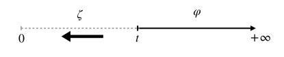
Figure 4.1: In the renormalisation group approach, the small scales $\zeta$ are averaged out and one considers the projection of the measure to the variables $\varphi$ encoding the large scales; in the figure above, the Polchinski flow goes from $0$ to $+\infty$. In fact, $\zeta$ and $\varphi$ play symmetric roles: in particular for $t=0$ the original measure is coded by $\varphi$, while instead for $t=+\infty$ the original measure is coded by $\zeta$. Stochastic localisation puts the emphasis on the variable $\zeta$ and therefore flows in the opposite direction (depicted by the thick arrow).

4.5.  Stochastic localisation perspective

The stochastic evolution (4.3) has so far been interpreted as the characteristics associated with the Polchinski equation (3.21). In this section, we are going to see that this stochastic process is also, after a suitable change of parametrisation, the flow of the stochastic localisation, introduced by Eldan. We refer to [40] for a survey on this method and its numerous applications in general, and to [28] for more specific developments on modified log-Sobolev inequalities. The relation between stochastic localisation and a semigroup approach was already pointed out in [58].

From Lemma 3.12, we recall that the gradient and Hessian of the renormalised potential $V_{t}$ can be interpreted as a mean and covariance of the fluctuation measure $\mu_{t}^{\varphi}$ defined in (3.17) by

(4.25) $$\bm{P}_{0,t}F(\varphi)=\mathbb{E}_{\mu_{t}^{\varphi}}[F].$$

The measure $\mu_{t}^{\varphi}$ is related to $\mu_{t}^{0}$ by the exponential tilt $e^{(C_{t}^{-1}\varphi,\zeta)}$, i.e., by the external field $C_{t}^{-1}\varphi$. In particular, by Lemma 3.12, the gradient of $V_{t}$ can be written as

(4.26) $$\nabla V_{t}(\varphi)=\mathbb{E}_{\mu_{t}^{\varphi}}[C_{t}^{-1}(\varphi-\zeta)]=C_{t}^{-1}(\varphi-\mathbb{E}_{\mu_{t}^{\varphi}}[\zeta])$$

where $\mathbb{E}_{\mu_{t}^{\varphi}}[\zeta]\in X$ is the mean of $\mu_{t}^{\varphi}$. The stochastic representation (4.3) can therefore be written in terms of the fluctuation measure instead of the renormalised potential. Indeed, let

(4.27) $$h_{t}=C_{t}^{-1}\varphi_{t},\qquad\mu_{t}=\mu_{t}^{\varphi_{t}}=\mu_{t}^{C_{t}h_{t}},\qquad\dot{\Sigma}_{t}=-\frac{\partial}{\partial t}C_{t}^{-1}=C_{t}^{-1}\dot{C}_{t}C_{t}^{-1}.$$

Since

(4.28) $$\dot{C}_{t}\nabla V_{t}(\varphi_{t})=\dot{C}_{t}C_{t}^{-1}(\varphi-\mathbb{E}_{\mu_{t}^{\varphi}}[\zeta])=C_{t}\dot{\Sigma}_{t}(\varphi-\mathbb{E}_{\mu_{t}^{\varphi}}[\zeta]),$$

the external field $h_{t}=C_{t}^{-1}\varphi_{t}$ satisfies the following SDE equivalent to (4.2): By the Itô formula (4.8) with $f(t,\varphi_{t})=C_{t}^{-1}\varphi_{t}$,

$$h_{t} =-\int_{t}^{\infty}df(u,\varphi_{u})$$

$$=\int_{t}^{\infty}\dot{\Sigma}_{u}\varphi_{u}\,du-\int_{t}^{\infty}C_{u}^{-1}\dot{C}_{u}\nabla V_{u}(\varphi_{u})\,du+\int_{t}^{\infty}C_{u}^{-1}\dot{C}_{u}^{1/2}dB_{u}$$

$$=\int_{t}^{\infty}\dot{\Sigma}_{u}\mathbb{E}_{\mu_{u}}[\zeta]\,du+\int_{t}^{\infty}C_{u}^{-1}\dot{C}_{u}^{1/2}dB_{u}$$

(4.29) $$=\int_{t}^{\infty}\dot{\Sigma}_{u}\mathbb{E}_{\mu_{u}}[\zeta]\,du+\int_{t}^{\infty}\dot{\Sigma}_{u}^{1/2}dB_{u},$$

where the last equality holds in distribution in the case that $\dot{C}_{u}$ and $C_{u}^{-1}$ do not commute.

What is known as stochastic localisation is the process $(h_{t})$ with the direction of time reversed. Thus in the stochastic localisation perspective, the renormalised potential and measure only play implicit roles, and the main object of study is the stochastic process (4.5) and the fluctuation measure (4.25). For this perspective, it is more convenient to assume that time is parameterised by $[0,T]$ (rather than our previous standard choice $[0,+\infty]$ — but again everything is reparametrisation invariant, so this is only for notational purposes). The fluctuation measure $\mu_{t}=\mu_{t}^{\varphi_{t}}$ then “starts” at the final time $t=T$ as the full measure of interest, and as $t$ decreases (time runs backwards) its fluctuations get absorbed into the renormalised measure $\nu_{t}$ until the fluctuation measure $\mu_{t}$ “localises” to a random Dirac measure $\mu_{0}=\delta_{\varphi_{0}}$ at time $t=0$, with $\varphi_{0}$ distributed according to the full measure $\nu_{0}=\mu_{T}$. See also Figure 4.1.

Although time runs backwards from $T$ to $0$ in the stochastic localisation perspective written with our time convention, let us change time direction to obtain a forward SDE and connect with the literature on stochastic localisation. Recalling (4.27), the initial measure $\nu_{0}=\mu_{T}$ coincides with the fluctuation measure at time $T$ as $h_{T}=0$. As done previously, we will always use tildes to denote change of time:

(4.30) $$\tilde{\varphi}_{t}=\varphi_{T-t},\quad\tilde{C}_{t}=C_{T-t},\quad\tilde{V}_{t}=V_{T-t},\quad\tilde{\mu}_{t}=\mu_{T-t},\qquad\tilde{h}_{t}=h_{T-t},\qquad\tilde{\dot{\Sigma}}_{t}=\dot{\Sigma}_{T-t}.$$

Using the notation ${\bf b}(\mu)=\mathbb{E}_{\mu}[\zeta]$ for the mean of $\mu$, the SDE (4.5) for $\tilde{h}$ can then be written as:

(4.31) $$d\tilde{h}_{t}=\tilde{\dot{\Sigma}}_{t}{\bf b}(\tilde{\mu}_{t})\,dt+\tilde{\dot{\Sigma}}_{t}^{1/2}d\tilde{B}_{t}.$$

This equation is the same as the stochastic localisation as it appears for example in [28, Fact 14] (after dropping tildes from the notation and with $y_{t}$ there corresponding to $\tilde{h}_{t}$).

The stochastic localisation perspective is different from our renormalisation group perspective in that the object of interest is (again) the fluctuation measure. For example, in the one-variable case $|\Lambda|=1$, starting from a measure $\tilde{\mu}_{0}(dx)=\nu_{0}(dx)\propto e^{-H(x)}$ (possibly log-concave), the strategy is to make it more convex by considering

(4.32) $$\tilde{\mu}_{t}(d\zeta)\propto e^{-H(\zeta)-\frac{t}{2}\zeta^{2}+\tilde{h}_{t}\zeta}\,d\zeta$$

with the choice of the process $\tilde{h}_{t}$ such that for any test function

(4.33) $$\forall t\geqslant 0,\qquad{\mathbb{E}}_{\nu_{0}}[F]={\mathbb{E}}\Big{[}{\mathbb{E}}_{\tilde{\mu}_{t}}(F)\Big{]}.$$

In this one variable example, the fluctuation measure above is the counterpart of (3.76) for the choice $C_{t}=1/(1+t)$ with $t$ decreasing from $+\infty$ to $0$ instead of $C_{t}=t$ with $t\in[0,1]$. With this reparametrisation, one gets from (4.27) that $\dot{\Sigma}_{t}=1$ so that

(4.34) $$t\geqslant 0,\qquad d\tilde{h}_{t}={\bf b}(\tilde{\mu}_{t})\,dt+d\tilde{B}_{t},\qquad\text{with}\quad\tilde{h}_{0}=0.$$

Starting from a general measure $\tilde{\mu}_{0}$, the primary concern in the stochastic localisation perspective is the measure $\tilde{\mu}_{t}$ which is now uniformly convex with Hessian at least $t$ (if say $H$ is log-concave), thus general concentration inequalities hold for the twisted measure and can be transferred to $\tilde{\mu}_{0}$ thanks to (4.33). For example, this is a key tool in current progress on the KLS conjecture, see [40] for a review. The larger $t$ is, the better in this respect. However, as $t$ grows the twisted measure $\tilde{\mu}_{t}(d\zeta)$ loses the features of the original $\tilde{\mu}_{0}$ so there is a trade-off in the choice of $t$. Contrary to our renormalisation point of view, in the stochastic localisation point of view, the distribution of $h_{t}=C_{t}^{-1}\varphi_{t}$ (which is given in terms of $\tilde{\mu}_{t}$ in (4.31) but can also be written in terms of our renormalised measure) does not play an important role (see Figure 4.1). The process $\tilde{h}_{t}$ is there to twist the measure and sometimes if one adds the correct $\dot{C}_{t}$ there are preferred directions to add the convexity.

5 Variational and transport perspectives on the Polchinski flow

In this section, we discuss transport-related perspectives on the Polchinski flow. We refer to [34] for additional perspectives such as an interpretation in terms of the Otto calculus that we do not discuss here.

5.1.  Föllmer’s problem

By (4.2), the distribution $\nu_{0}$ can be realised as the final time distribution $\varphi_{0}$ of the SDE:

(5.1) $$\varphi_{t}=-\int_{t}^{\infty}\dot{C}_{u}\nabla V_{u}(\varphi_{u})\,du+\int_{t}^{\infty}\sqrt{\dot{C}_{u}}\,dB_{u},$$

where we recall that the backwards SDE can be interpreted as in (4.14). One can ask whether the distribution $\nu_{0}$ can be obtained more efficiently if $\nabla V_{u}(\varphi_{u})$ is replaced by another drift $U_{u}(\varphi_{u})$, i.e., as the distribution of $\varphi_{0}^{U}$ when $\varphi^{U}$ is a strong solution of the SDE (again written backward in time):

(5.2) $$\varphi_{t}^{U}=-\int_{t}^{\infty}\dot{C}_{u}U_{u}(\varphi_{u}^{U})\,du+\int_{t}^{\infty}\sqrt{\dot{C}_{u}}\,dB_{u},$$

where the parameter $t$ takes values in $[0,+\infty]$ and $\varphi_{\infty}^{U}=0$. As pointed out in Remark 3.8, one could have also considered a parametrisation on a bounded time interval.

Denote by $\gamma_{0}=\mathsf{P}_{C_{\infty}}$ the distribution of the Gaussian reference measure, i.e., of $\int_{0}^{\infty}\sqrt{\dot{C}_{u}}\,dB_{u}$.

Theorem 5.1.

The gradient of the renormalised potential $V_{t}$ of the Polchinski flow (3.11) can be interpreted as the optimal drift in (5.2) in the following sense:

(5.3) $${\mathbb{H}}(\nu_{0}|\gamma_{0})=\frac{1}{2}{\mathbb{E}}\left[{\int_{0}^{\infty}|\nabla V_{t}(\varphi_{t})|_{{\dot{C}}_{t}}^{2}\,dt}\right]\leqslant\;\frac{1}{2}{\mathbb{E}}\left[{\int_{0}^{\infty}|U_{t}(\varphi_{t}^{U})|_{{\dot{C}}_{t}}^{2}\,dt}\right],$$

for any drift $U$ such that (5.2) has a strong solution with $\varphi_{0}\sim\nu_{0}$. Recall that $(\varphi_{t})$ follows (5.1).

Proof.

Let $U$ be a such that there is a strong solution $(\varphi_{t}^{U})$ of (5.2) with ${\mathbb{E}}\big{[}\int_{0}^{\infty}|U_{t}(\varphi_{t}^{U})|_{{\dot{C}}_{t}}^{2}\,dt\big{]}<\infty$. By construction $\varphi_{0}^{U}$ has law $\nu_{0}$ so that the relative entropy is given by

(5.4) $${\mathbb{H}}(\nu_{0}|\gamma_{0})=V_{\infty}(0)-{\mathbb{E}}[V_{0}(\varphi_{0}^{U})]=\int_{0}^{\infty}dt\;\frac{\partial}{\partial t}{\mathbb{E}}[V_{t}(\varphi_{t}^{U})],$$

with $\varphi^{U}$ evolving according to (5.2), and where we used that $\nu_{0}(d\varphi)=e^{+V_{\infty}(0)}e^{-V_{0}(\varphi)}\gamma_{0}(d\varphi)$ with normalisation factor given by $e^{-V_{\infty}(0)}=\mathsf{E}_{C_{\infty}}[{e^{-V_{0}(\zeta)}}]$ as in (3.13). The renormalised potential follows the Polchinski equation (3.21):

(5.5) $$\frac{\partial}{\partial t}V_{t}=\frac{1}{2}\Delta_{{\dot{C}}_{t}}V_{t}-\frac{1}{2}(\nabla V_{t})_{{\dot{C}}_{t}}^{2},\qquad(t\in(0,\infty)).$$

Therefore, by Itô’s formula,

$$\frac{\partial}{\partial t}{\mathbb{E}}[V_{t}(\varphi_{t}^{U})] ={\mathbb{E}}\left[{\frac{\partial}{\partial t}V_{t}(\varphi_{t}^{U})+\big{(}\nabla V_{t}(\varphi_{t}^{U}),U_{t}(\varphi_{t}^{U})\big{)}_{{\dot{C}}_{t}}-\frac{1}{2}\Delta_{{\dot{C}}_{t}}V_{t}(\varphi_{t}^{U})}\right]$$

$$={\mathbb{E}}\left[{-\frac{1}{2}(\nabla V_{t}(\varphi_{t}^{U}))_{{\dot{C}}_{t}}^{2}+\big{(}\nabla V_{t}(\varphi_{t}^{U}),U_{t}(\varphi_{t}^{U})\big{)}_{{\dot{C}}_{t}}}\right]$$

(5.6) $$=\frac{1}{2}{\mathbb{E}}\biggl{[}{-\big{(}\nabla V_{t}(\varphi_{t}^{U})-U_{t}(\varphi_{t}^{U})\big{)}^{2}_{{\dot{C}}_{t}}}\biggr{]}+\frac{1}{2}{\mathbb{E}}\biggl{[}{(U_{t}(\varphi_{t}^{U}))_{{\dot{C}}_{t}}^{2}}\biggr{]},$$

where we used the Polchinski equation (5.5) on the second line. Thus

(5.7) $$\frac{1}{2}{\mathbb{E}}\left[{\int_{0}^{\infty}(\nabla U_{t})_{{\dot{C}}_{t}}^{2}\,dt}\right]={\mathbb{H}}(\nu_{0}|\gamma_{0})+\frac{1}{2}{\mathbb{E}}\left[{\int_{0}^{\infty}\big{(}\nabla V_{t}-U_{t}\big{)}^{2}_{{\dot{C}}_{t}}\,dt}\right],$$

and the gradient of the renormalised potential $V_{t}$ provides the optimal drift. This completes the proof of Theorem 5.1. ∎

It turns out that the right-hand of (5.3) is, in fact, the relative entropy ${\mathbb{H}}({\bf Q}|{\bf P})$ of the path measure $\bf Q$ associated with (5.2) with respect to that of the Gaussian reference process $\bf P$.

Proposition 5.2.

The relative entropy of the path measure $\bf Q$ associated with a strong solution of (5.9) with respect to the path measure $\bf P$ of the Gaussian reference measure is given by

(5.8) $${\mathbb{H}}({\bf Q}|{\bf P})=\frac{1}{2}\,{\mathbb{E}}\left[{\int_{0}^{\infty}|U_{t}(\varphi_{t}^{U})|^{2}\,dt}\right].$$

Proof.

This is essentially a consequence of Girsanov’s theorem, see [63] for details. ∎

Since ${\mathbb{H}}({\bf Q}|{\bf P})\geqslant{\mathbb{H}}(\nu_{0}|\gamma_{0})$ always holds, by the entropy decomposition (2.5) and the fact that the laws of $\nu_{0}$ and $\gamma_{0}$ are marginals of the path measures ${\bf Q}$ and ${\bf P}$ respectively, the above shows that the optimal drift $U_{t}=\nabla V_{t}$ in fact achieves equality: ${\mathbb{H}}({\bf Q}|{\bf P})={\mathbb{H}}(\nu_{0}|\gamma_{0})$.

The above question was already studied by Föllmer [36], and we refer to [63] for an exposition of this and connections with Gaussian functional inequalities. Föllmer’s objective was to find the optimal drift $b_{t}$ such that the process $(X_{t})_{t\in[0,1]}$ defined by the following SDE and distributed at time $t=1$ according to a given target measure $\nu$:

(5.9) $$X_{0}=0,\quad dX_{t}=b_{t}(X_{t})\,dt+dB_{t}\quad\text{and}\quad X_{1}\sim\nu,$$

that minimises the dynamical cost

(5.10) $$\frac{1}{2}{\mathbb{E}}\left[{\int_{0}^{1}|b_{t}(X_{t})|^{2}\,dt}\right]$$

over all possible drifts $b$. Up to time reversal, parametrisation by $[0,+\infty]$ instead of $[0,1]$, and introduction of the covariances $\dot{C}_{t}$, this is exactly the set-up of (5.2). For us the introduction of the covariances $\dot{C}_{t}$ is a (conceptually and technically) important point, though, with the interpretation that the integral is now an integral over scales measured by the infinitesimal covariances $\dot{C}_{t}$ which can also be interpreted as metrics as in Section 3.6.

More generally, one can look for the optimal drift to built a target probability measure of the form $F(\varphi)\,\nu_{0}(d\varphi)$ using now the optimal stochastic flow as a reference process, i.e., we want to determine the drift $U$ such that for

(5.11) $$t\in[0,+\infty],\quad\psi_{t}=-\int_{t}^{\infty}{\dot{C}}_{s}U_{s}(\psi_{s})\,ds-\int_{t}^{\infty}{\dot{C}}_{s}\nabla V_{s}(\psi_{s})\,ds+\int_{t}^{\infty}\sqrt{{\dot{C}}_{s}}\,dB_{s},$$

the cost $\frac{1}{2}{\mathbb{E}}\big{[}\int_{0}^{1}|U_{t}(\psi_{t})|^{2}_{{\dot{C}}_{t}}dt\big{]}$ is minimised and $\psi_{0}$ is distributed according to $Fd\nu_{0}$. Proceeding as in the proof of Theorem 5.1, the optimal drift is given in terms of the Polchinski semigroup (3.12) as the gradient of

(5.12) $$W_{t}(\varphi)=-\log\bm{P}_{0,t}F(\varphi)=-V_{t}(\varphi)-\log\mathsf{E}_{C_{t}}\Big{[}F(\varphi+\zeta)e^{-V_{0}(\varphi+\zeta)}\Big{]}.$$

Thus one can check that

(5.13) $${\mathbb{H}}(F\nu_{0}|\nu_{0})=\operatorname{Ent}_{\nu_{0}}(F)=\frac{1}{2}{\mathbb{E}}\left[{\int_{0}^{\infty}|\nabla W_{t}(\varphi_{t})|_{{\dot{C}}_{t}}^{2}\,dt}\right].$$

In this way, we recover from (5.13) the entropy decomposition (3.44):

$$2\int_{0}^{\infty}\mathbb{E}_{\nu_{t}}\left[{|\nabla\sqrt{\bm{P}_{0,t}F}|_{\dot{C}_{t}}^{2}}\right]\,dt =\frac{1}{2}\int_{0}^{\infty}\mathbb{E}_{\nu_{t}}\left[{|\nabla\log\bm{P}_{0,t}F|_{\dot{C}_{t}}^{2}\;\bm{P}_{0,t}F}\right]\,dt$$

(5.14) $$=\frac{1}{2}{\mathbb{E}}\left[{\int_{0}^{\infty}|\nabla W_{t}(\varphi_{t})|_{{\dot{C}}_{t}}^{2}\,dt}\right],$$

where we used that the process (5.11) is distributed at time $t$ with density proportional to

(5.15) $$e^{-W_{t}(\varphi)-V_{t}(\varphi)}\mathsf{P}_{C_{\infty}-C_{t}}(d\varphi)\propto\bm{P}_{0,t}F(\varphi)\,\nu_{t}(d\varphi).$$

The above is an instance of the more general version of the Schrödinger problem which is to find the optimal drift so that the stochastic evolution (5.2) interpolates between two probability measures $\mu$ and $\nu$. Here, we discussed only the special case where the process starts from a Dirac measure $\mu=\delta_{0}$, and refer the reader to the survey [64] for a general overview and to [31] for a discussion on the role of the convexity of the potential.

In Section 5.3, we address a related issue, namely that in some cases, the previous flow can be modified in order to achieve an interpolation between the measure of interest and some Gaussian measure.

5.2.  Variational representation of the renormalised potential

Let $U_{t}=\nabla V_{t}(\varphi_{t})$ and recall that Proposition 4.3 states:

(5.16) $$V_{t}(\varphi)=\mathbb{E}_{\varphi_{t}=\varphi}\left[{V_{0}\Big{(}\varphi-\int_{0}^{t}\dot{C}_{s}U_{s}\,ds+\int_{0}^{t}\sqrt{\dot{C}_{s}}dW_{s}\Big{)}+\frac{1}{2}\int_{0}^{t}|U_{s}|^{2}_{\dot{C}_{s}}\,ds}\right].$$

In particular,

(5.17) $$V_{t}(\varphi)\geqslant\inf_{U}\mathbb{E}\left[{V_{0}\Big{(}\varphi-\int_{0}^{t}\dot{C}_{s}U_{s}\,ds+\int_{0}^{t}\sqrt{\dot{C}_{s}}dW_{s}\Big{)}+\frac{1}{2}\int_{0}^{t}|U_{s}|_{\dot{C}_{s}}^{2}\,ds}\right],$$

where the above infimum is over all adapted processes $U:[0,t]\to X$ (where adapted means backwards in time in our convention) called drifts. For our current purposes, it suffices to consider $U_{s}=U_{s}(\varphi_{s})$ associated with a strong solution to the (backward in time) SDE

(5.18) $$\varphi_{s}=\varphi-\int_{s}^{t}\dot{C}_{u}U_{u}(\varphi_{u})\,du+\int_{s}^{t}\sqrt{\dot{C}_{u}}\,dW_{u},\qquad(s\leqslant t).$$

The following proposition is a special case of the Boué-Dupuis or Borell formula, see [63], which gives equality in the infimum and is the starting point for the Barashkov–Gubinelli method [8]. An in-depth treatment of stochastic control problems of which this is a special case is given in [46].

Proposition 5.3.

(5.19) $$V_{t}(\varphi)=\inf_{U}\mathbb{E}\left[{V_{0}\Big{(}\varphi-\int_{0}^{t}\dot{C}_{s}U_{s}\,ds+\int_{0}^{t}\sqrt{\dot{C}_{s}}\,dW_{s}\Big{)}+\frac{1}{2}\int_{0}^{t}|U_{s}|_{\dot{C}_{s}}^{2}\,ds}\right].$$

Sketch.

The entropy inequality (2.62) with $G(\zeta)=-V_{0}(\varphi+\zeta)$ applied to the Gaussian measure $\mathsf{P}_{C_{t}}$ implies that for any density $F$ with $\mathsf{E}_{C_{t}}[F]=1$:

(5.20) $$V_{t}(\varphi)=-\log\mathsf{E}_{C_{t}}[e^{-V_{0}(\varphi+\zeta)}]\leqslant\operatorname{Ent}_{\mathsf{P}_{C_{t}}}(F)+\mathsf{E}_{C_{t}}\left[{F(\zeta)V_{0}(\varphi+\zeta)}\right].$$

Given any drift $U_{s}$, let $F\,d\mathsf{P}_{C_{t}}$ denote the law of $\varphi_{0}-\varphi$ solving (5.18):

(5.21) $$\varphi_{0}-\varphi=-\int_{0}^{t}\dot{C}_{s}U_{s}\,ds+\int_{0}^{t}\sqrt{\dot{C}_{s}}\,dW_{s}.$$

Then

(5.22) $$V_{t}(\varphi)\leqslant\mathbb{E}\left[{\frac{1}{2}\int_{0}^{t}|U_{s}(\varphi_{s})|_{\dot{C}_{s}}^{2}\,ds+V_{0}\Big{(}\varphi-\int_{0}^{t}\dot{C}_{s}U_{s}\,ds+\int_{0}^{t}\sqrt{\dot{C}_{s}}\,dW_{s}\Big{)}}\right],$$

where we used that the entropy is bounded by the first term, exactly as in Theorem 5.1. As already discussed, the converse direction follows from Proposition 4.3. ∎

The point of view is now that by estimating the expectation on the right-hand side above, for a general drift $U$, one can obtain estimates on $V_{t}(\varphi)$, and in particular on $V_{\infty}(\varphi)$ which we recall from (3.2) is equivalent to the logarithmic moment generating function of the measure $\nu_{0}$. For further details and application to construction of the $\varphi^{4}_{d}$ measures, we refer to [8, 9].

5.3.  Lipschitz transport

Instead of a stochastic process, one could also define a map $\hat{S}_{t}:X\mapsto X$ transporting $\nu_{0}$ to some measure $\hat{\nu}_{t}$ in order to recover functional inequalities for $\nu_{0}$ from $\hat{\nu}_{t}$. For example, assume that $\hat{\nu}_{t}$ satisfies a log-Sobolev inequality with constant $\gamma$ and that

(5.23) $$\mathbb{E}_{\nu_{0}}\left[{F(\varphi)}\right]=\mathbb{E}_{\nu_{t}}\left[{F\big{(}\hat{S}_{t}(\varphi)\big{)}}\right].$$

If the Jacobian $\nabla\hat{S}_{t}$ is bounded by some constant $C$ in the following sense

(5.24) $$\forall\omega\in X,\quad(\nabla\hat{S}_{t}\,\omega)^{2}\leqslant C^{2}(\omega)^{2},$$

then $\nu_{0}$ satisfies also a log-Sobolev inequality

$$\operatorname{Ent}_{\nu_{0}}\left[{F(\varphi)}\right] =\mathbb{E}_{\hat{\nu}_{t}}[\Phi(F\circ\hat{S}_{t})]-\Phi(\mathbb{E}_{\hat{\nu}_{t}}[F\circ\hat{S}_{t}])$$

$$\leqslant\frac{2}{\gamma}\mathbb{E}_{\hat{\nu}_{t}}\left[{(\nabla\sqrt{F\circ\hat{S}_{t}})^{2}}\right]=\frac{2}{\gamma}\mathbb{E}_{\hat{\nu}_{t}}\left[{\big{(}^{t}\nabla\hat{S}_{t}\,(\nabla\sqrt{F})(\hat{S}_{t})\big{)}^{2}}\right]$$

(5.25) $$\leqslant\frac{2C^{2}}{\gamma}\mathbb{E}_{\hat{\nu}_{t}}\left[{\big{(}(\nabla\sqrt{F})(\hat{S}_{t})\big{)}^{2}}\right]=\frac{2C^{2}}{\gamma}\mathbb{E}_{\nu_{0}}\left[{(\nabla\sqrt{F})^{2}}\right],$$

where we used that $\nabla\hat{S}_{t}$ and its transpose ${}^{t}\nabla\hat{S}_{t}$ have the same operator norm. An analogous argument can be applied to more general functional inequalities.

This line of research was first investigated in [25] where it was understood that a convex perturbation of a Gaussian measure leads to a $1$-Lipschitz transport map $\hat{S}_{t}$. We refer to [57, 75, 71, 72, 58, 82, 44] for more recent developments as well as other applications of the Lipschitz properties of transport maps to functional inequalities. In this section, we follow the work [83] which derived a Lipschitz estimate of the form (5.24) from the multiscale criterion (3.32) for some covariance decomposition, and generalise the result to other decompositions.

Recall that the measure $\nu_{0}$ gets renormalised to $\nu_{t}$ by the Polchinski flow. By construction $\mathbb{E}_{\nu_{t}}[\cdot]=\mathsf{E}_{C_{\infty}-C_{t}}[e^{-V_{t}}\cdot]$ and $\nu_{t}$ converges to a Dirac mass. As the measure $\nu_{t}$ degenerates, it is more convenient to consider the measure $\hat{\nu}_{t}$ obtained by rescaling $\nu_{t}$ by some matrix $D_{t}$ so that the measures $\nu_{0}$ and $\hat{\nu}_{t}$ are comparable:

(5.26) $$\mathbb{E}_{\hat{\nu}_{t}}\left[{F(\varphi)}\right]=\mathbb{E}_{\nu_{t}}\left[{F(D_{t}\varphi)}\right].$$

If $V_{0}=0$, a natural choice for $D_{t}$ is to preserve the Gaussian measure, i.e.,

(5.27) $$D_{t}^{-1}(C_{\infty}-C_{t})^{-1}D_{t}^{-1}=A\quad\Rightarrow\quad D_{t}AD_{t}=(C_{\infty}-C_{t})^{-1},$$

where all inverse are understood to be taken on the range of $A$. This is implicitly assumed in the rest of the section, with $\mspace{2.0mu}\mathrm{i}\mspace{-0.6mu}\mathrm{d}$ also denoting the identity matrix on the range of $A$. Assuming that all the matrices depend smoothly on $t$ and commute, then the choice (5.27) implies the following useful relation:

(5.28) $$2D_{t}^{-1}\dot{D}_{t}=\dot{C}_{t}(C_{\infty}-C_{t})^{-1}=\dot{C}_{t}D_{t}AD_{t}.$$

Using again (5.27) we get (recall $C_{0}=0$ and notice $D_{0}=\mspace{2.0mu}\mathrm{i}\mspace{-0.6mu}\mathrm{d}$):

(5.29) $$\frac{\partial}{\partial t}(D_{t}^{-2})=-A\dot{C}_{t}\quad\Rightarrow\quad D_{t}=(\mspace{2.0mu}\mathrm{i}\mspace{-0.6mu}\mathrm{d}-AC_{t})^{-1/2}.$$

By construction $\lim_{t\to\infty}D_{t}^{-1}\varphi=0$ and the renormalised potential satisfies $\lim_{t\to\infty}V_{t}(D_{t}^{-1}\varphi)=V_{\infty}(0)$ (because $\operatorname{Hess}V_{t}\leqslant C_{t}^{-1}\leqslant C_{1}^{-1}$ for $t\geqslant 1$, recall Lemma 3.12). Thus the following convergence in distribution to a Gaussian measure holds:

(5.30) $$\lim_{t\to\infty}\mathbb{E}_{\hat{\nu}_{t}}\left[{F(\varphi)}\right]=\mathsf{E}_{C_{\infty}}\left[{F(\varphi)}\right]=\mathsf{E}_{A^{-1}}\left[{F(\varphi)}\right].$$

Consider $S_{t}$ a transport map between $\nu_{0}$ and $\hat{\nu}_{t}$, so that

(5.31) $$\mathbb{E}_{\nu_{0}}\left[{F\big{(}S_{t}(\varphi)\big{)}}\right]=\mathbb{E}_{\hat{\nu}_{t}}\left[{F(\varphi)}\right]=\mathbb{E}_{\nu_{t}}\left[{F(D_{t}\varphi)}\right].$$

Note that ultimately we are interested in $\hat{S}_{t}$ which is the inverse of $S_{t}$, see (5.23).

We are going to determine an evolution for $S_{t}:X\mapsto X$. On the one hand,

(5.32) $$\frac{\partial}{\partial t}\mathbb{E}_{\nu_{0}}\left[{F\big{(}S_{t}(\varphi)\big{)}}\right]=\mathbb{E}_{\nu_{0}}\left[{\big{(}\nabla F\big{(}S_{t}(\varphi)\big{)},\partial_{t}S_{t}(\varphi)\big{)}}\right],$$

and on the other hand from (3.27):

(5.33) $$\frac{\partial}{\partial t}\mathbb{E}_{\nu_{t}}\left[{F(D_{t}\varphi)}\right]=\mathbb{E}_{\nu_{t}}\left[{-\bm{L}_{t}F(D_{t}\varphi)+(\dot{D}_{t}\varphi,\nabla F(D_{t}\varphi))}\right],$$

with $\bm{L}_{t}F=\frac{1}{2}\Delta_{\dot{C}_{t}}F-(\nabla V_{t},\nabla F)_{\dot{C}_{t}}$. Integrating by parts, this gives

$$\frac{\partial}{\partial t}\mathbb{E}_{\nu_{t}}\left[{F(D_{t}\varphi)}\right] =\mathbb{E}_{\nu_{t}}\left[{\frac{1}{2}(\dot{C}_{t}\nabla V_{t}(\varphi)-\frac{1}{2}\dot{C}_{t}\,(C_{\infty}-C_{t})^{-1}\varphi+D_{t}^{-1}\dot{D}_{t}\varphi,D_{t}\nabla F(D_{t}\varphi))}\right]$$

$$=\mathbb{E}_{\nu_{t}}\left[{\frac{1}{2}(\nabla V_{t}(\varphi),D_{t}\nabla F(D_{t}\varphi))_{\dot{C}_{t}}}\right]$$

(5.34) $$=\mathbb{E}_{\nu_{0}}\left[{\frac{1}{2}(\nabla V_{t}(D_{t}^{-1}\cdot),D_{t}\nabla F)_{\dot{C}_{t}}(S_{t}(\varphi))}\right],$$

where we used (5.28). Thus the evolution of $S_{t}$ is given by

(5.35) $$\frac{\partial}{\partial t}S_{t}(\varphi)=\frac{1}{2}D_{t}\,\dot{C}_{t}\nabla V_{t}(D_{t}^{-1}S_{t}(\varphi)).$$

It was realised in [83] that for the choice $\dot{C}_{t}=e^{-tA}$ (often used in applications, see Section 6) the Lipschitz structure associated with $S_{t}$ is directly related to (a variant of) the multiscale Bakry–Émery criterion (3.32).

Theorem 5.4 (​​[83]).

Under the assumption

(5.36) $$\forall\varphi\in X:\qquad\dot{C}_{t}^{1/2}\operatorname{Hess}V_{t}(\varphi)\dot{C}_{t}^{1/2}\geqslant\dot{\mu}_{t}\mspace{2.0mu}\mathrm{i}\mspace{-0.6mu}\mathrm{d},\quad\text{with}\quad\mu_{t}:=\int_{0}^{t}ds\,\dot{\mu}_{s},$$

the inverse map $\hat{S}_{t}=S_{t}^{-1}:X\mapsto X$ is $\exp(-\frac{1}{2}\mu_{t})$-Lipschitz.

From the convergence (5.30) to the Gaussian measure and if $\mu_{\infty}:=\int_{0}^{\infty}ds\,\dot{\mu}_{s}<\infty$, then from the previous theorem, one can extract a $\exp(-\frac{1}{2}\mu_{\infty})$-Lipschitz map from the Gaussian measure ${\sf P}_{C_{\infty}}$ to $\nu_{0}$ (see [75, Lemma 2.1]).

Proof.

For $\dot{C}_{t}=e^{-tA}$, the definition (5.29) implies $D_{t}=e^{\frac{1}{2}tA}=\dot{C}_{t}^{-1/2}$ and the evolution (5.35) becomes particularly simple:

(5.37) $$\frac{\partial}{\partial t}S_{t}(\varphi)=\frac{1}{2}\dot{C}_{t}^{1/2}\nabla V_{t}\big{(}\dot{C}_{t}^{1/2}S_{t}(\varphi)\big{)}.$$

The Jacobian evolves according to

(5.38) $$\frac{\partial}{\partial t}\nabla S_{t}(\varphi)=\frac{1}{2}\dot{C}_{t}^{1/2}\operatorname{Hess}V_{t}\big{(}\dot{C}_{t}^{1/2}S_{t}(\varphi)\big{)}\dot{C}_{t}^{1/2}\nabla S_{t}(\varphi).$$

As a consequence of (5.36), the Gronwall inequality implies

(5.39) $$\forall\omega\in X,\quad\frac{\partial}{\partial t}(\nabla S_{t}(\varphi)\omega)^{2}\geqslant\dot{\mu}_{t}(\nabla S_{t}(\varphi)\omega)^{2}\quad\Rightarrow\quad(\nabla S_{t}(\varphi)\omega)^{2}\geqslant\exp(\mu_{t})(\omega)^{2}.$$

By the inverse function theorem, we deduce that the operator norm of $\nabla\hat{S}_{t}$ is less than $\exp(-\frac{1}{2}\mu_{t})$. ∎

Another useful covariance decomposition (see Theorem 6.2) is of the form $\dot{C}_{t}=(tA+\mspace{2.0mu}\mathrm{i}\mspace{-0.6mu}\mathrm{d})^{-2}$. The result of Theorem 5.4 can be extended to that case, but with a worse Lipschitz constant.

Theorem 5.5.

Let $\dot{C}_{t}=(tA+1)^{-2}$ for $t\geqslant 0$. Under the assumption

(5.40) $$\forall\varphi\in X:\qquad\dot{C}_{t}\operatorname{Hess}V_{t}(\varphi)\dot{C}_{t}-\frac{1}{2}\ddot{C}_{t}\geqslant\dot{\lambda}_{t}\dot{C}_{t},\quad\text{with}\quad\lambda_{t}:=\int_{0}^{t}ds\,\dot{\lambda}_{s},$$

the inverse map $\hat{S}_{t}=S_{t}^{-1}:X\mapsto X$ is $\big{(}\sqrt{t\|A\|+1}\,\big{)}e^{-\lambda_{t}/2}$-Lipschitz, with $\|M\|=\sup\{\|M\omega\|_{2}:\omega\in X,\|\omega\|_{2}=1\}$ the operator norm of a matrix $M$.

Remark 5.6.

In concrete examples, the $\lambda_{t}$ diverge with $t$, contrary to the $\mu_{t}$ in Theorem 5.4 that remained bounded. This divergence precisely compensates the factor $\sqrt{t}$, giving a uniform Lipschitz bound on $\hat{S}_{t}$. An application of Theorem 5.5 is given in Proposition 6.3.

Proof of Theorem 5.5.

For each $t\geqslant 0$, we look for a matrix $B_{t}$ depending only on $C_{t}$ and its derivatives, commuting with them, and such that we can set up a Gronwall estimate for $(B_{t}\nabla S_{t}(\varphi)\omega)^{2}$ for each $\varphi,\omega\in X$. Note that the definition (5.29) of $D_{t}$ implies $D_{t}=\dot{C}_{t}^{-1/4}$. In particular $D_{t}$ commutes with $B_{s},C_{s},\dot{C}_{s},\ddot{C}_{s}$ for any $s$.

Equation (5.35) gives:

(5.41) $$\frac{\partial}{\partial t}\nabla S_{t}(\varphi)=\frac{1}{2}\dot{C}_{t}D_{t}\operatorname{Hess}V_{t}(D_{t}^{-1}S_{t}(\varphi))D_{t}^{-1}\nabla S_{t}(\varphi).$$

Therefore:

(5.42) $$\frac{\partial}{\partial t}\big{(}B_{t}\nabla S_{t}(\varphi)\omega\big{)}^{2}=\Big{(}B_{t}\nabla S_{t}(\varphi)\omega,\Big{[}B_{t}\dot{C}_{t}D_{t}\operatorname{Hess}V_{t}(D_{t}^{-1}S_{t}(\varphi))D_{t}^{-1}B_{t}^{-1}+2\dot{B_{t}}B_{t}^{-1}\Big{]}B_{t}\nabla S_{t}(\varphi)\omega\Big{)}.$$

In order to use the Hessian bound (5.40), we need to choose $B_{t}$ in such a way that, for each $t\geqslant 0$:

$$B_{t}\dot{C}_{t}D_{t}\operatorname{Hess}V_{t}(D_{t}^{-1}S_{t}(\varphi))D_{t}^{-1}B_{t}^{-1}+2\dot{B_{t}}B_{t}^{-1}$$

(5.43) $$\qquad\geqslant\dot{C}_{t}^{1/2}\operatorname{Hess}V_{t}(D_{t}^{-1}S_{t}(\varphi))\dot{C}_{t}^{1/2}-\frac{1}{2}\dot{C}_{t}^{-1/2}\ddot{C}_{t}\dot{C}_{t}^{-1/2}.$$

The Hessian term gives $B_{t}=D_{t}^{-1}\dot{C}_{t}^{-1/2}=\dot{C}_{t}^{-1/4}=D_{t}$ as a sufficient condition, and for this choice $\dot{B}_{t}B_{t}^{-1}=-\frac{1}{4}\ddot{C}_{t}\dot{C}_{t}^{-1}$ so that (5.43) holds. As a result,

(5.44) $$\frac{\partial}{\partial t}\big{(}D_{t}\nabla S_{t}(\varphi)\omega\big{)}^{2}\geqslant\dot{\lambda}_{t}\big{(}D_{t}\nabla S_{t}(\varphi)\omega\big{)}^{2},\qquad(t\geqslant 0).$$

The Gronwall inequality then yields:

(5.45) $$\big{(}D_{t}\nabla S_{t}(\varphi)\omega\big{)}^{2}\geqslant e^{\lambda_{t}}(\omega)^{2},\qquad(t\geqslant 0).$$

It follows that $\hat{S}_{t}$ is $\|\dot{C}_{t}^{1/4}\|e^{-\lambda_{t}/2}$-Lipschitz, i.e., $\big{(}\sqrt{t\|A\|+1}\,\big{)}e^{-\lambda_{t}/2}$-Lipschitz as claimed. ∎

6 Applications

In this section, we present concrete examples to which the multiscale Bakry-Émery criterion of Theorem 3.6 can be applied. The criterion gives a bound on the log-Sobolev constant in terms of real numbers $\dot{\lambda}_{t}$ ($t>0$) obtained through convexity lower bounds on the renormalised potential:

(6.1) $$\forall\varphi\in X,t\geqslant 0:\qquad\dot{C}_{t}\operatorname{Hess}V_{t}(\varphi)\dot{C}_{t}-\frac{1}{2}\ddot{C}_{t}\geqslant\dot{\lambda}_{t}\dot{C}_{t}.$$

These lower bounds are determined by the choice of the covariance decomposition $(C_{t})$. While Theorem 3.6 holds for any decomposition, checking (6.1) for concrete models often requires a specific choice of decomposition. This will be illustrated in examples in the following sections.

For now, we discuss the sharpness of the criterion in Theorem 3.6. To fix ideas, suppose we have a model defined on $\Lambda_{\varepsilon,L}=L\mathbb{T}^{d}\cap\varepsilon\mathbb{Z}^{d}$ for $d\geqslant 2$, where either $\varepsilon=1$ is fixed and $L\to\infty$ (statistical mechanics model) or $\varepsilon\to 0$ is a small regularisation parameter and $L$ is fixed or $L\to\infty$ (continuum field theory model in finite or infinite volume). From the discussion in Sections 2.6–2.7 recall that the speed of convergence of an associated dynamics is often related to the presence of phase transitions in equilibrium. These phase transitions are phenomena arising in the limit of large volumes, i.e., large $L$. In this limit, one typically expects that the log-Sobolev constant should be bounded from below independently of $\Lambda_{\varepsilon,L}$ as long as no phase transition occurs. On the other hand, the additional regularisation parameter $\varepsilon>0$ is not expected to affect the dynamics, i.e., the log-Sobolev constant should also be bounded from below as $\varepsilon\to 0$.

Sharpness of the criterion of Theorem 3.6 is therefore evaluated through the following questions:

1. In absence of a phase transition, does the criterion provide a lower bound on the log-Sobolev constant uniform in the volume (i.e., in $L$)?

2. Does it give a bound on the log-Sobolev constant independent of the regularisation parameter $\varepsilon$ for continuum models?

3. If the first point holds, can one correctly estimate how the log-Sobolev constant vanishes as a function of the distance to the critical point, or at the critical point as a function of $L$?

The third point is considerably more involved than the first two. To provide a guideline to read the next sections, we collect here the answers to the above three questions obtained by studying the examples presented below.

• For statistical mechanics models ($\varepsilon=1$) at high temperature, i.e., far away from the critical point, the multiscale Bakry-Émery criterion implies point (i), see, e.g., Theorem 6.7 which extends to a much broader class of models. This regime is also covered by many other criteria (see e.g. the monographs [80, 51] and [90]), with the notable exception of mean-field spin-glass models, see the discussion of [11].

• The criterion (6.1) can be sharp enough to reach the critical point, see, e.g., Theorem 6.13 and Proposition 6.3 below for the Ising and $\varphi^{4}$ models. In other words, there are models for which the criterion implies (i) up to the phase transition. We expect that the criterion should imply (i) up to the critical point for a large class of models.

• The criterion can provide a bound on the log-Sobolev constant that is uniform as $\varepsilon\to 0$ (see Theorems 6.1 and 6.2 for the $\varphi^{4}$ and sine-Gordon models), thus satisfying point (ii).

Point (iii) is in general open and in this generality hopelessly difficult, but some positive results exist. For models with quadratic mean-field interaction such as the Curie-Weiss model, one can answer (iii) in the affirmative. A detailed analysis above and below the critical temperature was also carried out for mean-field $O(n)$ models in [21]. For certain continuum particle systems with mean-field interaction, the behaviour close to the critical point is the subject of ongoing work [14]. For more complicated models in which computations can be carried out, such as the hierarchical $\varphi^{4}_{4}$ model [12], the criterion provides almost matching upper and lower bounds on how fast the log-Sobolev constant vanishes at the critical point. For the nearest-neighbour Ising model in $d\geqslant 5$, the criterion implies polynomial bounds on the log-Sobolev constant at and near the critical temperature [18].

6.1.  Applications to Euclidean field theory

In this section, let $\Lambda=\Lambda_{\varepsilon,L}$ be a discrete torus of mesh size $\varepsilon$ and side length $L$ (assumed to be a multiple of $\varepsilon$): $\Lambda_{\varepsilon,L}=L\mathbb{T}^{d}\cap\varepsilon\mathbb{Z}^{d}$. The discrete Laplacian on $\Lambda_{\varepsilon,L}$ is given by

(6.2) $$\forall\varphi\in\mathbb{R}^{\Lambda_{\varepsilon,L}},\qquad(\Delta^{\varepsilon}\varphi)_{x}=\varepsilon^{-2}\sum_{y\sim x}(\varphi_{y}-\varphi_{x}).$$

The (lattice regularised) Euclidean field theory models we consider are of the form

(6.3) $$\nu^{\varepsilon,L}(d\varphi)\propto\exp\bigg{[}-\frac{\varepsilon^{d}}{2}\sum_{x\in\Lambda_{\varepsilon,L}}\varphi_{x}(-\Delta^{\varepsilon}\varphi)_{x}+\varepsilon^{d}\sum_{x\in\Lambda_{\varepsilon,L}}V^{\varepsilon}(\varphi_{x})\bigg{]}\,d\varphi,$$

where $d\varphi$ denotes the Lebesgue measure on $\mathbb{R}^{\Lambda_{\varepsilon,L}}$ and $V^{\varepsilon}$ is a real-valued function chosen in such a way that the $\varepsilon\rightarrow 0$ limit of the measure (on a suitable space of generalised functions) exists and is non-Gaussian. Writing $\nabla V^{\varepsilon}(\varphi)=((V^{\varepsilon})^{\prime}(\varphi_{x}))_{x}$ for $\varphi\in\mathbb{R}^{\Lambda_{\varepsilon,L}}$, the dynamics is the singular SPDE

(6.4) $$d\varphi_{t}=\Delta^{\varepsilon}\varphi_{t}\,dt-\nabla V^{\varepsilon}(\varphi_{t})\,dt+\sqrt{2}dW_{t}^{\varepsilon,L}$$

where $dW_{t}^{\varepsilon,L}$ is space-time white noise on $\mathbb{R}_{+}\times\Lambda_{\varepsilon,L}$, i.e., the $W^{\varepsilon,L}_{x}$ are independent Brownian motions with variance $\varepsilon^{-d}$ for $x\in\Lambda_{\varepsilon,L}$, or equivalently a standard Brownian motion with respect to the continuum inner product $(u,v)_{\varepsilon}=\varepsilon^{d}\sum_{x\in\Lambda_{\varepsilon,L}}u_{x}v_{x}$. The pathwise (short time) limit theory for such SPDEs is the subject of Hairer’s regularity structure theory [54, 52, 53], the paracontrolled method of Gubinelli et al. [50, 26, 92], and the pathwise renormalisation group approach [61, 39]. The log-Sobolev inequality for the associated dynamics takes the form:

(6.5) $$\operatorname{Ent}_{\nu^{\varepsilon,L}}(F)\leqslant\frac{2}{\gamma}D_{\nu^{\varepsilon,L}}(\sqrt{F}),$$

with the standard Dirichlet form with respect to the gradient $\nabla_{\varepsilon}$ corresponding to $(\cdot,\cdot)_{\varepsilon}$:

(6.6) $$D_{\nu^{\varepsilon,L}}(F)=\mathbb{E}_{\nu^{\varepsilon,L}}\Bigl{[}{(\nabla^{\varepsilon}F,\nabla^{\varepsilon}F)_{\varepsilon}}\Bigr{]}=\frac{1}{\varepsilon^{d}}\sum_{x\in\Lambda_{\varepsilon,L}}\mathbb{E}_{\nu^{\varepsilon,L}}\Bigg{[}\bigg{|}\frac{\partial F}{\partial\varphi_{x}}\bigg{|}^{2}\Bigg{]},$$

i.e., $(\nabla^{\varepsilon}F)_{x}=(\nabla_{\varphi}^{\varepsilon}F)_{x}=\varepsilon^{-d}\frac{\partial F}{\partial\varphi_{x}}$. (Thus this gradient acts on functionals of fields $F:\mathbb{R}^{\Lambda_{\varepsilon,L}}\to\mathbb{R}$ while the Laplacian (6.2) acts on fields $\varphi\in\mathbb{R}^{\Lambda_{\varepsilon,L}}$.)

We now discuss two prototypical models.

Continuum sine-Gordon model

Let $d=2$. For $0<\beta<8\pi$ and $z\in\mathbb{R}$, the sine-Gordon model is defined by the potential

(6.7) $$V^{\varepsilon}(\varphi)=2z\varepsilon^{-\beta/4\pi}\cos(\sqrt{\beta}\varphi),\qquad(\varphi\in\mathbb{R}).$$

One can also add a convex quadratic part to the measure: the massive sine-Gordon model with mass $m>0$ corresponds to the potential $V^{\varepsilon}(\varphi)+\frac{1}{2}m^{2}\varphi^{2}$.

Continuum $\varphi^{4}$ model

Let $d=2$ or $d=3$. For $\lambda>0$ and $\mu\in\mathbb{R}$, the $\varphi^{4}_{d}$ measure is defined by

(6.8) $$V^{\varepsilon}(\varphi)=\frac{\lambda}{4}\varphi^{4}+\frac{\mu+a^{\varepsilon}(\lambda)}{2}\varphi^{2},\qquad(\varphi\in\mathbb{R}),$$

where $a^{\varepsilon}(\lambda)$ is a divergent counterterm. Explicitly, for an arbitrary fixed $m^{2}>0$, one can take $a^{\varepsilon}(\lambda)=a^{\varepsilon}(\lambda,m^{2})$ with

(6.9) $$a^{\varepsilon}(\lambda,m^{2}):=-3\lambda\big{(}-\Delta^{\varepsilon}+m^{2})^{-1}(0,0)+6\lambda^{2}\big{\|}\big{(}-\Delta^{\varepsilon}+m^{2}\big{)}^{-1}(0,\cdot)\big{\|}^{3}_{L^{3}(\Lambda_{\varepsilon,L})},$$

and the notation $\|f\|^{p}_{L^{p}(\Lambda_{\varepsilon,L})}=\varepsilon^{d}\sum_{x\in\Lambda_{\varepsilon,L}}|f(x)|^{p}$ for $p>0$. The counterterms defined in terms of different $m^{2}$ differ by additive constants and thus the choice of $m^{2}$ corresponds to a normalisation. In the following we take $m^{2}=1$ for the definition of the counterterm.

The sine-Gordon and $\varphi^{4}_{d}$ models are defined on the discretised torus $\Lambda_{\varepsilon,L}=L\mathbb{T}^{d}\cap\varepsilon\mathbb{Z}^{d}$. As explained in Section 2.7, these models should be thought of as discretised versions of limiting models defined on the continuum torus $L\mathbb{T}^{d}$. Recall that the criterion of Theorem 3.6 asks for a lower bound on the Hessian of the renormalised potential uniformly in the field: for some $\dot{\lambda}_{t}\in\mathbb{R}$,

(6.10) $$\forall\varphi\in\mathbb{R}^{\Lambda_{\varepsilon,L}},t\geqslant 0:\qquad\dot{C}_{t}\operatorname{Hess}V_{t}(\varphi)\dot{C}_{t}-\frac{1}{2}\ddot{C}_{t}\geqslant\dot{\lambda}_{t}\dot{C}_{t}.$$

To obtain information on the dynamics in the $\varepsilon\to 0$ limit, one is therefore interested in estimates of the renormalised potential that are uniform in $\varepsilon,\varphi$.

For the sine-Gordon model, this was carried out in [13] by providing an explicit description of the renormalised potential at each scale.

Theorem 6.1.

For the massive continuum sine-Gordon model with mass $m>0$, let $A=-\Delta^{\varepsilon}+m^{2}\mspace{2.0mu}\mathrm{i}\mspace{-0.6mu}\mathrm{d}$ and $\dot{C}_{t}=e^{-tA}$ ($t\geqslant 0$). Then, if $\beta<6\pi$, there is a constant $\mu^{*}=\mu^{*}(\beta,z,m,L)>0$ that does not depend on $\varepsilon,t$, such that with $V_{0}(\varphi)=\varepsilon^{2}\sum_{x\in\Lambda_{\varepsilon,L}}2z\cos(\sqrt{\beta}\varphi_{x})$:

(6.11) $$\forall\varphi\in\mathbb{R}^{\Lambda_{\varepsilon,L}},t\geqslant 0:\qquad\dot{C}_{t}\operatorname{Hess}V_{t}(\varphi)\dot{C}_{t}\geqslant\dot{\mu}_{t}\dot{C}_{t}\quad\text{with}\quad\sup_{t\geqslant 0}\Big{|}\int_{0}^{t}\dot{\mu}_{s}ds\Big{|}\leqslant\mu^{*}.$$

Given $\beta,z,m,L$, this yields a lower bound on the log-Sobolev constant $\inf_{\varepsilon}\gamma^{\varepsilon,L}_{\beta,z,m}>0$.

Moreover, the log-Sobolev constant is uniform in the large-scale parameter $L$ under the following condition. If $L$ satisfies $m\geqslant 1/L$ and the coupling constant $z$ is such that $|z|\leqslant\delta_{\beta}m^{2+\beta/4\pi}$ for a small enough $\delta_{\beta}>0$, then $\inf_{\varepsilon}\gamma^{\varepsilon,L}_{\beta,z,m}>m^{2}-O_{\beta}\big{(}m^{\beta/4\pi}|z|\big{)}$, uniformly in $L$.

For the sine-Gordon model, the multiscale Bakry-Émery criterion of Theorem 3.6 is thus seen to provide the optimal independence of $\varepsilon$ of the log-Sobolev constant in finite volume, as well as of $L$ under an additional small coupling assumption depending on the external mass.

In the case of the $\varphi^{4}_{d}$ model, a description of the renormalised potential at all scales is more difficult to work out directly. The log-Sobolev inequality was obtained in [19] using a correlation inequality due to Ding, Song, and Sun [38], valid for ferromagnetic interactions (see Proposition 6.12 below). This correlation inequality reduces the proof of the log-Sobolev constant to an estimate of certain correlation functions at field $\varphi=0$, for which many tools are available.

Theorem 6.2.

For the continuum $\varphi^{4}$ model in $d=2,3$, let $A=-\Delta^{\varepsilon}+\mspace{2.0mu}\mathrm{i}\mspace{-0.6mu}\mathrm{d}$ and $\dot{C}_{t}=(tA+\mspace{2.0mu}\mathrm{i}\mspace{-0.6mu}\mathrm{d})^{-2}$ ($t\geqslant 0$) and take $m=1$ in the definition (6.9) of the counterterm. Then with $V_{0}(\varphi)=\varepsilon^{d}\sum_{x\in\Lambda_{\varepsilon,L}}(\frac{\lambda}{4}\varphi^{4}+\frac{\mu-1+a^{\varepsilon}(\lambda)}{2}\varphi^{2})$:

(6.12) $$\forall\varphi\in\mathbb{R}^{\Lambda_{\varepsilon,L}},t\geqslant 0:\qquad\dot{C}_{t}\operatorname{Hess}V_{t}(\varphi)\dot{C}_{t}-\frac{1}{2}\ddot{C}_{t}\geqslant\Big{(}\frac{1}{t}-\frac{\chi_{t}}{t^{2}}\Big{)}\dot{C}_{t},$$

with $\chi_{t}=\chi^{\varepsilon,L}_{\lambda,\mu+1/t}$ the 0-field susceptibility of the $\varphi^{4}_{d}$ model at scale $t>0$: if $\big{<}\cdot\big{>}^{\varepsilon,L}_{\lambda,\mu}$ denotes the average under the $\varphi^{4}_{d}$ measure,

(6.13) $$\chi_{t}:=\varepsilon^{d}\sum_{x\in\Lambda_{\varepsilon,L}}\big{<}\varphi_{0}\varphi_{x}\big{>}^{\varepsilon,L}_{\lambda,\mu+1/t}.$$

This implies that the log-Sobolev constant $\gamma^{\varepsilon,L}_{\lambda,\mu}$ satisfies $\inf_{\varepsilon,L}\gamma^{\varepsilon,L}_{\lambda,\mu}>0$ for any $\lambda,\mu$ for which the measure does not have a phase transition, and $\inf_{\varepsilon}\gamma^{\varepsilon,L}_{\lambda,\mu}>0$ for any $\lambda,\mu$ and $L$ fixed.

In the $\varphi^{4}_{d}$ case, the multiscale criterion gives a log-Sobolev constant bounded uniformly in the volume and $\varepsilon$ in the entire single-phase region. However, the bound obtained on the log-Sobolev constant has accurate dependence on $\lambda,\mu$ only far away from the transition, corresponding to values of $\lambda,\mu$ such that $\mu>0$ and when $\lambda\ll\mu$.

We conclude the section with a last example, the lattice $\varphi^{4}$ model, corresponding to the case $\varepsilon=1$ above. Thus its single-site potential is given by:

(6.14) $$V(\varphi)=V^{\varepsilon=1}(\varphi)=\frac{g}{4}\varphi^{4}+\frac{\nu}{2}\varphi^{2},$$

and the coupling matrix is $A=-\Delta^{\varepsilon=1}+\mspace{2.0mu}\mathrm{i}\mspace{-0.6mu}\mathrm{d}$ setting $m^{2}=1$ without loss of generality. The state space is $L\mathbb{T}^{d}\cap\mathbb{Z}^{d}$ for any $d\geqslant 1$. As a special case, Theorem 6.2 yields the log-Sobolev inequality whenever the infinite volume susceptibility is finite (though the proof of this statement can be simplified considerably in this case, see [19, Example 3.1]). We nonetheless make an independent statement because the Lipschitz constant of the map of Theorem 5.5 can be bounded uniformly in the volume. Theorem 5.5 does not seem to be effective for the discrete model.

Example 6.3 (​​[19, Example 3.1]).

For the lattice $\varphi^{4}$ model in any dimension with associated expectation $\big{<}\cdot\big{>}^{L}_{g,\nu}$, let $\dot{C}_{t}=(tA+\mspace{2.0mu}\mathrm{i}\mspace{-0.6mu}\mathrm{d})^{-2}$ and define the lattice susceptibility:

(6.15) $$\chi^{L}_{t}:=\sum_{x\in\Lambda}\big{<}\varphi_{0}\varphi_{x}\big{>}^{L}_{g,\nu+1/t}.$$

Then the Hessian bound (6.12) holds with $\chi^{L}_{t}$ in the right-hand side instead of $\chi_{t}$. This implies that the log-Sobolev constant $\gamma^{L}_{g,\nu}$ satisfies $\inf_{L}\gamma^{L}_{g,\nu}>0$ if and only if $\sup_{L}\chi^{L}_{\infty}<\infty$.

Moreover, if $\sup_{L}\chi^{L}_{\infty}<\infty$, then the transport map of Theorem 5.5 has Lipschitz constant is bounded uniformly in $L$ and $t$.

Proof.

Let us prove the bound on the Lipschitz constant. Theorem 5.5 gives the following bound on the Lipschitz constant of the transport map:

(6.16) $$\sqrt{t\|A\|+1}\exp\Big{[}-\frac{1}{2}\int_{0}^{t}\Big{(}\frac{1}{s}-\frac{\chi^{L}_{s}}{s^{2}}\Big{)}\,ds\Big{]}.$$

The Brascamp-Lieb inequality (3.63) ensures:

(6.17) $$\inf_{L}\inf_{s\leqslant 1}\Big{(}\frac{1}{s}-\frac{\chi^{L}_{s}}{s^{2}}\Big{)}>0.$$

For $t\geqslant 1$, the second Griffiths inequality [48] implies that $t\mapsto\chi^{L}_{t}$ is increasing, thus is bounded by $\chi^{L}_{\infty}$ so that

(6.18) $$\frac{1}{t}-\frac{\chi^{L}_{t}}{t^{2}}\geqslant\frac{1}{t}-\frac{\chi^{L}_{\infty}}{t^{2}},\qquad(t\geqslant 1).$$

Combining the previous inequalities, we deduce that there is a constant $C=C(\chi^{L}_{\infty})>0$ such that for all $t>0$:

(6.19) $$\exp\Big{[}-\frac{1}{2}\int_{0}^{t}\Big{(}\frac{1}{s}-\frac{\chi^{L}_{s}}{s^{2}}\,ds\Big{)}\Big{]}\leqslant C\min\big{\{}t^{-1/2},1\big{\}},$$

and the observation $\|A\|\leqslant\|-\Delta^{\varepsilon=1}+\mspace{2.0mu}\mathrm{i}\mspace{-0.6mu}\mathrm{d}\|\leqslant 4d+1$ implies that the Lipschitz constant (6.16) is uniformly bounded. This concludes the proof. ∎

6.2.  Applications to Ising models

In this section, we explain how to apply the ideas developed in Section 3 to Ising models with discrete spins. Using the Bakry–Émery criterion and its multiscale version, these ideas were developed in [11, 18], while closely related results were obtained using spectral and entropic independence and stability estimates in [41, 3, 28].

6.2.1. Renormalised potential

The Ising model with coupling matrix $A$ at inverse temperature $\beta>0$ and (site-dependent) external field $h$ on a finite set $\Lambda$ is defined by:

(6.20) $$\mathbb{E}_{\mu}[F]=\mathbb{E}_{\mu_{\beta,h}}[F]\propto\sum_{\sigma\in\{\pm 1\}^{\Lambda}}e^{-\frac{1}{2}(\sigma,\beta A\sigma)+(h,\sigma)}F(\sigma).$$

Since $\sigma_{x}^{2}=1$ for each $x$, the measure is invariant under the change $A\to A+\alpha\mspace{2.0mu}\mathrm{i}\mspace{-0.6mu}\mathrm{d}$, $\alpha\in\mathbb{R}$. Without loss of generality, we can thus assume that the coupling matrix $A$ is positive definite. We also assume that it has spectral radius bounded by $1$; this just amounts to a choice of normalisation for $\beta$. A natural covariance decomposition is

(6.21) $$C_{t}=(tA+(\alpha-t)\mspace{2.0mu}\mathrm{i}\mspace{-0.6mu}\mathrm{d})^{-1},$$

for a parameter $\alpha>0$ which will be unimportant. For $t<\alpha$ the matrix $C_{t}$ is positive definite and for $\beta<\alpha$, as explained above, the Ising model at inverse temperature $\beta$ can be written as

(6.22) $$\mathbb{E}_{\mu}[F]\propto\sum_{\sigma\in\{\pm 1\}^{\Lambda}}e^{-\frac{1}{2}(\sigma,C_{\beta}^{-1}\sigma)+(h,\sigma)}F(\sigma).$$

Strictly speaking, $C_{t}$ is not a covariance decomposition since $C_{0}=\alpha^{-1}\mspace{2.0mu}\mathrm{i}\mspace{-0.6mu}\mathrm{d}\neq 0$, different from the assumption in Section 3. However, all results from that section can be applied to the covariance decomposition $C_{t}-C_{0}$, and we will do this without further emphasis. The renormalised potential can be defined analogously to the continuous setting as:

(6.23) $$V_{t}(\varphi)=-\log\sum_{\sigma\in\{\pm 1\}^{\Lambda}}e^{-\frac{1}{2}(\sigma-\varphi,C_{t}^{-1}(\sigma-\varphi))+(h,\sigma)}.$$

This leads to a decomposition of the Ising measure (6.20) as:

(6.24) $$\mathbb{E}_{\mu}[F]=\mathbb{E}_{\nu_{t,\beta}}\big{[}\mathbb{E}_{\mu_{t}^{\varphi}}[F]\big{]}\qquad(0\leqslant t<\beta).$$

By analogy with (3.18), the fluctuation measure $\mu^{\varphi}_{t}$ used above is the Ising measure with coupling matrix $C_{t}^{-1}$ and external field $C_{t}^{-1}\varphi+h$:

(6.25) $$\mu^{\varphi}_{t}(\sigma)=\mu_{t,C_{t}^{-1}\varphi+h}\propto e^{-\frac{1}{2}(\sigma,C_{t}^{-1}\sigma)+(C_{t}^{-1}\varphi+h,\sigma)},$$

and the renormalised measure $\nu_{t}=\nu_{t,\beta}$ is supported on the image of $C_{\beta}-C_{t}$ in $\mathbb{R}^{\Lambda}$:

(6.26) $$\nu_{t,\beta}(d\varphi)\propto e^{-V_{t}(\varphi)}\,\mathsf{P}_{C_{\beta}-C_{t}}(d\varphi)\propto\exp\left[{-\frac{1}{2}(\varphi,(C_{\beta}-C_{t})^{-1}\varphi)-V_{t}(\varphi)}\right]\,d\varphi.$$

Even though $\sigma:\Lambda\to\{\pm 1\}$ is discrete, the renormalised field $\varphi:\Lambda\to\mathbb{R}$ is continuous as soon as $t>0$. Convexity-based criterions, such as the Bakry-Émery or multiscale Bakry-Émery criterions of Theorems 2.8 and 3.6, can therefore be used to derive log-Sobolev inequalities for $\nu_{t,\beta}$.

Before discussing these, we summarise results about the infinite temperature (product) Ising model, which serve as input to these arguments.

6.2.2. Preliminaries: single-spin inequalities

At infinite temperature $\beta=0$ the spin models we consider become product measures. By tensorisation, it thus suffices to know the log-Sobolev constant of a single spin (see Example 2.9). The following summarises known results for these.

Ising model, standard Dirichlet form

Let $\mu$ be the probability measure on $\{\pm 1\}$ with $\mu(+1)=p=1-q$. The standard Dirichlet form is

(6.27) $$D_{\mu}(F)=\frac{1}{2}\mathbb{E}_{\mu}(F(\sigma^{x})-F(\sigma))^{2}=\frac{1}{2}(F(+1)-F(-1))^{2}.$$

Proposition 6.4.

Let $\mu$ be the probability measure on $\{\pm 1\}$ with $\mu(+1)=p=1-q$. Then

(6.28) $$\operatorname{Ent}_{\mu}(F)\leqslant\frac{pq(\log p-\log q)}{p-q}(\sqrt{F(+1)}-\sqrt{F(-1)})^{2}.$$

Thus the log-Sobolev constant with respect to the standard Dirichlet form on $\{\pm 1\}$ is at least $2$:

(6.29) $$\operatorname{Ent}_{\mu}(F)\leqslant D(\sqrt{F})=\frac{2}{\gamma_{0}}D(\sqrt{F}),\qquad\gamma_{0}=2.$$

Proof.

The proof can be found in [81] or [5]. ∎

Ising model, heat bath Dirichlet form

With $\mu$ as above, the heat-bath Dirichlet form is

(6.30) $$D^{\rm HB}(F)=\frac{1}{2}\sum_{\sigma}\frac{\mu(\sigma)\mu(\sigma^{x})}{\mu(\sigma)+\mu(\sigma^{x})}(F(\sigma^{x})-F(\sigma))^{2}=pq(F(+1)-F(-1))^{2}$$

Proposition 6.5.

Let $\mu$ be the probability measure on $\{\pm 1\}$ with $\mu(+1)=p=1-q$. Then

(6.31) $$\operatorname{Ent}_{\mu}(F)\leqslant pq(\log F(+1)-\log F(-1))(F(+1)-F(-1)).$$

Thus the modified log-Sobolev constant with respect to the heat-bath Dirichlet form is at least $1/2$:

(6.32) $$\operatorname{Ent}_{\mu}F\leqslant D^{\rm HB}(\log F,F)=\frac{1}{2\gamma_{0}}D^{\rm HB}(\log F,F),\qquad\gamma_{0}=\frac{1}{2}.$$

Proof.

See [22, Example 3.8]. ∎

Similar single-spin inequalities are available for $O(n)$ models [91, 84] and allow to extend for example Theorem 6.7 below for the Ising model to these models with little change [11].

6.2.3. Entropy decomposition

To prove a log-Sobolev inequality (or modified log-Sobolev inequality) for the Ising measure, we start from the decomposition (6.24) with $t=0$, decomposing $\mu=\mu_{\beta}^{0}$ into two parts: an infinite temperature Ising measure $\mu^{\varphi}_{0}$ with external field $C_{0}^{-1}\varphi+h$ and the renormalised measure $\nu_{0,\beta}$. The corresponding entropy decomposition (2.5) is:

(6.33) $$\operatorname{Ent}_{\mu}(F)=\mathbb{E}_{\nu_{0,\beta}}[\operatorname{Ent}_{\mu_{0}^{\varphi}}(F)]+\operatorname{Ent}_{\nu_{0,\beta}}\big{(}\mathbb{E}_{\mu_{0}^{\varphi}}[F]\big{)}.$$

To prove the log-Sobolev inequality (or modified log-Sobolev inequality) with respect to a Dirichlet form $D_{\mu}$, we want to bound both terms by a multiple of $D_{\mu}(\sqrt{F})$ (or $D_{\mu}(F,\log F)$). In this discussion, we focus on the log-Sobolev inequality with respect to the standard Dirichlet form:

(6.34) $$D_{\mu}(F)=\frac{1}{2}\sum_{x\in\Lambda}\mathbb{E}_{\mu}\Bigl{[}{(F(\sigma)-F(\sigma^{x}))^{2}}\Bigr{]}.$$

However, the same strategy applies with different jump rates and a modified log-Sobolev inequality or a spectral inequality as input (and output), see Sections 6.2.2 and 6.2.5.

Under the assumption that $\mu_{0}^{\varphi}$ satisfies a log-Sobolev inequality with constant $\gamma_{0}$ uniformly in $\varphi$, the first term on the right-hand side of (6.33) is bounded by

(6.35) $$\frac{2}{\gamma_{0}}\mathbb{E}_{\nu_{0,\beta}}[D_{\mu_{0}^{\varphi}}(\sqrt{F})]=\frac{2}{\gamma_{0}}D_{\mu}(\sqrt{F}).$$

Since $\mu_{0}^{\varphi}$ is a product measure, this assumption is well understood and one can take $\gamma_{0}=2$ for the standard Dirichlet form, as discussed in Section 6.2.2. The last equality relies on the specific jump rates in the standard Dirichlet form (6.34). For other Dirichlet forms, one can also get an inequality, see Section 6.2.5.

Bounding the second term on the right-hand side of (6.33) essentially amounts to estimating the log-Sobolev constant of the renormalised measure $\nu_{0,\beta}$. Indeed, if $\nu_{0,\beta}$ satisfies a log-Sobolev inequality with constant $\gamma_{0,\beta}$ (and standard Dirichlet form) then this term is bounded by

(6.36) $$\frac{2}{\gamma_{0,\beta}}\mathbb{E}_{\nu_{0,\beta}}\Big{[}\big{|}\big{(}\nabla_{\varphi}\mathbb{E}_{\mu^{\varphi}_{0}}[F]^{1/2}\big{)}\big{|}^{2}\Big{]}\leqslant\frac{4\alpha^{2}}{\gamma_{0}\gamma_{0,\beta}}D_{\mu}(\sqrt{F}),$$

where the second inequality is elementary and follows from the next exercise (which is similar to the argument in the tensorisation proof of Example 2.9) and the Cauchy–Schwarz inequality.

Exercise 6.6.

For each $x\in\Lambda$, let $\mu^{\varphi,x}_{0}$ denote the law of $\sigma_{x}$ under the product measure $\mu^{\varphi}_{0}$. Then:

(6.37) $$\nabla_{\varphi_{x}}\big{(}\mathbb{E}_{\mu^{\varphi}_{0}}[F]^{1/2}\big{)}=\frac{\alpha}{2\sqrt{\mathbb{E}_{\mu^{\varphi}_{0}}[F]}}\operatorname{Cov}_{\mu^{\varphi}_{0}}(F,\sigma_{x})=\frac{\alpha}{2\sqrt{\mathbb{E}_{\mu^{\varphi}_{0}}[F]}}\mathbb{E}_{\mu_{0}^{\varphi}}\Big{[}\operatorname{Cov}_{\mu^{\varphi,x}_{0}}(F,\sigma_{x})\Big{]}$$

(recall $C_{0}=\alpha^{-1}\mspace{2.0mu}\mathrm{i}\mspace{-0.6mu}\mathrm{d}$) and:

(6.38) $$\operatorname{Cov}_{\mu^{\varphi,x}_{0}}(F,\sigma_{x})^{2}\leqslant 8\mathbb{E}_{\mu_{0}^{\varphi,x}}[F]\operatorname{Var}_{\mu^{\varphi,x}_{0}}(\sqrt{F})\leqslant\frac{8}{\gamma_{0}}\mathbb{E}_{\mu_{0}^{\varphi,x}}[F]D_{\mu^{\varphi,x}_{0}}(\sqrt{F}).$$

Sketch.

The first equation is a simple computation. The first inequality in (6.38) follows from Cauchy-Schwarz inequality using the following general expression for the covariance of functions $G_{1},G_{2}$ under a measure $m$:

(6.39) $$\operatorname{Cov}_{m}(G_{1},G_{2})=\frac{1}{2}\int\big{(}G_{1}(x)-G_{1}(y)\big{)}\big{(}G_{2}(x)-G_{2}(y)\big{)}\,dm(x)\,dm(y).$$

The second inequality is the general fact that the spectral gap is always larger than the log-Sobolev constant, see Proposition 2.5. Details can be found in [11]. ∎

In summary, if $\mu_{0}^{\varphi}$ satisfies a log-Sobolev inequality with constant $\gamma_{0}$ and $\nu_{0,\beta}$ satisfies a log-Sobolev inequality with constant $\gamma_{0,\beta}$ then the inverse log-Sobolev constant $\gamma^{-1}$ of $\mu$ satisfies

(6.40) $$\frac{1}{\gamma}\leqslant\frac{1}{\gamma_{0}}\left[{1+\frac{2\alpha^{2}}{\gamma_{0,\beta}}}\right].$$

At this point the objective is to bound the log-Sobolev constant $\gamma_{0,\beta}$ of the renormalised measure $\nu_{0,\beta}$. Results are stated next under different conditions, with the corresponding verifications postponed to Section 6.2.4.

Recall that the renormalised measure is $\nu_{0,\beta}(d\varphi)\propto e^{-V_{0}(\varphi)}\mathsf{P}_{C_{\beta}-C_{0}}(d\varphi)$ with the renormalised potential $V_{0}$ defined in (6.23). If the temperature is sufficiently high, namely if $\beta<\alpha<1$, then it turns out that $V_{0}$ is strictly convex so that the standard Bakry–Émery criterion is applicable [11] and gives (see Exercise 6.10):

(6.41) $$\gamma_{0,\beta}\geqslant\alpha-\alpha^{2}.$$

Taking $\alpha\downarrow\beta$, this leads to the following theorem. We recall the convention fixed below (6.20) that the coupling matrix $A$ has spectrum in $[0,1]$. This spectral condition appeared in [11] (and unlike previously existing conditions applies to the SK spin glass).

Theorem 6.7 (Spectral high temperature condition [11]).

For $\beta<1$ (under the conventions stated below (6.20)), the Ising model $\mu$ satisfies the log-Sobolev inequality: for each $F:\{-1,1\}^{\Lambda}\to\mathbb{R}_{+}$,

(6.42) $$\operatorname{Ent}_{\mu}(F)\leqslant\Big{(}1+\frac{2\beta}{1-\beta}\Big{)}D_{\mu}(\sqrt{F}).$$

For $\beta>1$, the renormalised potential $V_{0}$ is in general not convex and the log-Sobolev constant $\gamma_{0,\beta}$ of the renormalised measure $\nu_{0,\beta}$ cannot be bounded using the Bakry–Émery criterion. However, the argument above can be generalised by using the multiscale Bakry–Émery criterion instead. Assuming $\dot{\lambda}_{t}$ are as in the multiscale Bakry–Émery condition (6.1), Theorem 3.6 gives:

(6.43) $$\frac{1}{\gamma_{0,\beta}}\leqslant|\dot{C}_{0}|\int_{0}^{\beta}e^{-2\lambda_{t}\,dt}=\frac{1}{\alpha^{2}}\int_{0}^{\beta}e^{-2\lambda_{t}}\,dt,\qquad\lambda_{t}=\int_{0}^{t}\dot{\lambda}_{s}\,ds,$$

and substituting this into (6.40) gives the following log-Sobolev inequality:

(6.44) $$\operatorname{Ent}_{\mu}(F)\leqslant\frac{2}{\gamma}D_{\mu}(\sqrt{F}),\qquad\frac{1}{\gamma}\leqslant\frac{1}{\gamma_{0}}\left[{1+2\int_{0}^{\beta}e^{-2\lambda_{t}}dt}\right],\qquad\lambda_{t}=\int_{0}^{t}\dot{\lambda}_{s}\,ds.$$

In the same situation, instead of using the multiscale Bakry–Émery criterion to bound $\gamma_{0,\beta}$ in (6.40), one can prove a log-Sobolev inequality for $\mu$ by using the entropic stability estimate discussed in Section 3.7. This was done in [28] (to prove a modified log-Sobolev inequality, but the argument generalises to a log-Sobolev inequality for the standard Dirichlet form, see below). It turns out that, for the decomposition (6.21), the conditions (3.32) and (3.107) of the multiscale Bakry–Émery criterion and of the entropic stability estimate are identical provided $\dot{\lambda}_{t}=-\alpha_{t}$, see Exercise 6.11. This is not the case for other covariance decompositions, and in particular not for those used for continuous models, see the discussion in Section 3.7. Using the entropic stability estimate (3.109), the entropy is therefore bounded by:

(6.45) $$\operatorname{Ent}_{\mu}(F)\leqslant e^{-\lambda_{\beta}}\mathbb{E}_{\nu_{0,\beta}}[\operatorname{Ent}_{\mu_{0}^{\varphi}}(F)],\qquad\lambda_{t}=\int_{0}^{t}\dot{\lambda}_{s}\,ds,$$

and with the uniform log-Sobolev inequality for $\mu_{0}^{\varphi}$ this gives

(6.46) $$\operatorname{Ent}_{\mu}(F)\leqslant\frac{2}{\gamma}D_{\mu}(\sqrt{F}),\qquad\frac{1}{\gamma}\leqslant\frac{1}{\gamma_{0}}e^{-\lambda_{\beta}},\qquad\lambda_{t}=\int_{0}^{t}\dot{\lambda}_{s}\,ds.$$

This estimate is very similar to the estimate (6.44) obtained using the multiscale Bakry–Émery criterion, but not exactly identical. Both estimates can be applied up to the critical point in a very general setting for ferromagnetic Ising models and yield a polynomial bound on the log-Sobolev constant under the mean-field bound which holds on $\Lambda\subset\mathbb{Z}^{d}$ in $d\geqslant 5$, see Theorem 6.13 below. The strategies of the two proofs have different advantages. We summarise the results as follows.

Theorem 6.8 (Covariance conditions for Ising models [18, 28]).

The log-Sobolev constant of the Ising model at inverse temperature $\beta$ is bounded by (6.44) or (6.46).

As discussed previously, we formulated the results for the log-Sobolev inequality with respect to the standard Dirichlet form. This is a canonical choice (as already explained in Section 2.2), but the argument can be adapted easily to other choices of jump rates with the conclusion of a possibly modified log-Sobolev inequality, see Section 6.2.5. As pointed out in [41], other choices are of interest when the jump rates are unbounded.

6.2.4. Hessian of the renormalised potential and covariance

In both strategies, using the multiscale Bakry–Émery criterion or the entropic stability estimate, the estimate of the log-Sobolev constant reduces to estimating the constants $\dot{\lambda}_{t}=-\alpha_{t}$ bounding the Hessian of the renormalised potential from below. From Lemma 3.12, recall that these estimates are equivalent to bounds on the covariance of the fluctuation measure, a point of view that is particularly useful for the Ising model. Indeed, the Hessian of the renormalised potential can be represented as follows.

Exercise 6.9.

Show that

(6.47) $$\operatorname{Hess}V_{t}(\varphi)=C_{t}^{-1}-C_{t}^{-1}\Sigma_{t}(C_{t}^{-1}\varphi+h)C_{t}^{-1},$$

where $\Sigma_{t}(g)=(\operatorname{Cov}_{\mu_{t,g}}(\sigma_{x},\sigma_{y}))_{x,y\in\Lambda}$ is the covariance matrix of the Ising model $\mu_{t,g}$ at inverse temperature $t$ and site-dependent magnetic field $g$ (so that (6.25) reads $\mu_{t}^{\varphi}=\mu_{t,C_{t}^{-1}\varphi+h}$).

For $\beta<1$, one can obtain the following convexity directly from this representation, which allows to apply the standard Bakry–Émery criterion to derive (6.41) and conclude the proof of Theorem 6.7.

Exercise 6.10.

Let $1\geqslant\alpha>\beta$, and set $C_{t}=(tA+(\alpha-t)\mspace{2.0mu}\mathrm{i}\mspace{-0.6mu}\mathrm{d})^{-1}$. Then $V_{t}$ is convex for all $t\in[0,\alpha]$.

Proof.

Since $\mu_{0,g}$ is a product measure and $|\sigma_{x}|\leqslant 1$,

(6.48) $$\Sigma_{0}(g)=\operatorname{diag}(\operatorname{Var}_{\mu_{0,g}}(\sigma_{x}))_{x\in\Lambda}\leqslant\mspace{2.0mu}\mathrm{i}\mspace{-0.6mu}\mathrm{d}.$$

Using that $C_{0}=\alpha^{-1}\mspace{2.0mu}\mathrm{i}\mspace{-0.6mu}\mathrm{d}$, we deduce from (6.47) that

(6.49) $$\operatorname{Hess}V_{0}(\varphi)=\big{(}\alpha-\alpha^{2}\Sigma_{0}(\alpha\varphi+h)\big{)}\mspace{2.0mu}\mathrm{i}\mspace{-0.6mu}\mathrm{d}\geqslant(\alpha-\alpha^{2})\mspace{2.0mu}\mathrm{i}\mspace{-0.6mu}\mathrm{d}.$$

Thus if $\alpha\leqslant 1$, it follows that $V_{0}$ is convex. By Proposition 3.13, $V_{t}$ is convex for all $t>0$. ∎

For general $\beta>0$, the semi-convexity criterion of the Hessian can be equivalently formulated as covariance estimate uniformly in an external field.

Exercise 6.11.

From $C_{t}=(tA+(\alpha-t)\mspace{2.0mu}\mathrm{i}\mspace{-0.6mu}\mathrm{d})^{-1}$, one has $\dot{C}_{t}=(\mspace{2.0mu}\mathrm{i}\mspace{-0.6mu}\mathrm{d}-A)C_{t}^{2}$, $\ddot{C}_{t}=2(\mspace{2.0mu}\mathrm{i}\mspace{-0.6mu}\mathrm{d}-A)\dot{C}_{t}C_{t}$ and thus the multiscale Bakry–Émery criterion (3.32) and the entropic stability criterion (3.107) hold with $-\dot{\lambda}_{t}=\alpha_{t}=\bar{\chi}_{t}$ where $\bar{\chi}_{t}$ is a uniform upper bound on the spectral radius of the covariance matrix of an Ising model uniformly in an external field:

(6.50) $$\bar{\chi}_{t}=\sup_{g\in\mathbb{R}^{\Lambda}}\chi_{t}(g),\qquad\chi_{t}(g)=\|\Sigma_{t}(g)\|.$$

Now a significant simplification occurs for Ising models with ferromagnetic interaction, meaning $A_{x,y}\leqslant 0$ for $x\neq y$. This includes the case of the lattice Laplacian $\Delta\sigma_{x}=\sum_{y\sim x}[\sigma_{y}-\sigma_{x}]$. For ferromagnetic interactions, it turns out that the spectral radius is maximal at $0$ field:

(6.51) $$\bar{\chi}_{t}=\chi_{t}(0).$$

This is a consequence of the FKG inequality (which implies that the covariance matrix has pointwise nonnegative coefficients), the Perron–Frobenious theorem (which therefore implies that the largest eigenvector has nonnegative entries), and the following remarkable correlation inequality due to Ding–Song–Sun [18] which implies that the covariance between any two spins is maximised at $0$ field.

Proposition 6.12 (Ding–Song–Sun inequality [38, Corollary 1.3]).

Let $\mu=\mu_{\beta,h}$ be the Ising measure (6.20) with ferromagnetic interaction $A$, and external field $h\in[-\infty,\infty]^{\Lambda}$, with values $\pm\infty$ corresponding to boundary conditions. Then:

(6.52) $$\operatorname{Cov}_{\mu_{\beta,h}}(\sigma_{x},\sigma_{y})\leqslant\operatorname{Cov}_{\mu_{\beta,0}}(\sigma_{x},\sigma_{y})=\mathbb{E}_{\mu_{\beta,0}}[\sigma_{x}\sigma_{y}],\qquad(x,y\in\Lambda).$$

In particular, if the interaction $A$ is ferromagnetic and (for simplicity) in addition translation invariant, i.e., $A_{x,y}=A_{x-y}$, then

(6.53) $$\bar{\chi}_{t}=\chi_{t}=\chi_{t}(0)=\sum_{x\in\Lambda}\mathbb{E}_{\mu_{t,0}}[\sigma_{x}\sigma_{y}]$$

is the susceptibility of the Ising model. It characterises the phase transition of the ferromagnetic Ising model, in the sense that, e.g., for $\Lambda\subset\mathbb{Z}^{d}$ ($d\geqslant 2$), the critical value $\beta_{c}$ of $\beta$ satisfies:

(6.54) $$\beta_{c}:=\sup\left\{{\beta>0:\sup_{\Lambda\uparrow\mathbb{Z}^{d}}\sum_{x\in\Lambda}\mathbb{E}_{\mu_{\beta,0}}[\sigma_{0}\sigma_{x}]<\infty}\right\}.$$

By combining the Ding–Song–Sun correlation bound with the multiscale Bakry–Émery criterion, and in view of the above characterisation of $\beta_{c}$, the following log-Sobolev inequality up to the critical point for ferromagnetic Ising models on general geometries was proven in [18].

Theorem 6.13 (​​[18, Theorem 1.1]).

The log-Sobolev constant $\gamma_{\beta,h}$ of the Ising measure (6.20) with ferromagnetic interaction satisfies:

(6.55) $$\frac{1}{\gamma_{\beta,h}}\leqslant\frac{1}{2}+\int_{0}^{\beta}e^{2\int_{0}^{t}\chi_{s}\,ds}\,dt,$$

with $\chi_{\beta}=\sup_{x}\sum_{y}\mathbb{E}_{\mu_{\beta,0}}[\sigma_{x}\sigma_{y}]$ or more generally the largest eigenvalue of $(\mathbb{E}_{\mu_{\beta,0}}[\sigma_{x}\sigma_{y}])_{x,y}$.

The above result implies that $\gamma_{\beta,h}$ is bounded below uniformly in the size of the lattice as long as $\beta<\beta_{c}$. For special geometries, this could already be argued from [38] (which establishes the strong spatial mixing property).

More interesting is the fact that (6.55) also gives an explicit bound on the log-Sobolev constant. For Ising models with mean-field interactions, the bound implies that $\gamma_{\beta,h}$ is of order $\beta_{c}-\beta$, which is the correct scaling. More significantly, the bound (6.55) implies a polynomial bound on $1/\gamma_{\beta,h}$ on $\Lambda\subset\mathbb{Z}^{d}$ in dimension five and higher (and more generally under the so-called mean-field bound on the susceptibility, i.e., when the susceptibility diverges linearly), where polynomial means as a function of $\beta_{c}-\beta$ when $\beta<\beta_{c}$, and of the lattice size when $\beta=\beta_{c}$. The degree of this polynomial is not expected to be sharp unless $D=1$.

Example 6.14.

If $\chi_{\beta}\leqslant D/(\beta_{c}-\beta)$ then $\gamma_{\beta,h}$ is bounded polynomially in $\beta_{c}-\beta$, and if $\chi_{\beta}\leqslant D/(\beta_{c}-\beta+L^{-\alpha})$ then $\gamma_{\beta_{c},h}$ is polynomial in $L$. These assumptions hold for the ferromagnetic nearest-neighbour Ising model on $\Lambda\subset\mathbb{Z}^{d}$ when $d\geqslant 5$ [1].

Similarly, one can recover the main result of [73] from (6.55), which improves the high temperature condition of (6.42) in the case of ferromagnetic Ising models on graphs with maximal degree $d$ (for the mixing time and spectral gap). For the ferromagnetic Ising model, $A$ is the negative adjacency matrix of the graph which we now (for comparison) do not normalise to have spectrum contained in $[0,1]$. The condition of (6.42) cannot be improved for general non-ferromagnetic interactions with bounded spectral radius, but for ferromagnetic models the condition established in [73] is $\beta<\operatorname{artanh}(1/(d-1))$, whereas the condition of (6.42) translates in this case to $\beta<1/(2d)$. The value $\beta_{u}=\operatorname{artanh}(1/(d-1))$ is the uniqueness threshold for the ferromagnetic Ising model on the infinite $d$-regular tree and also the critical point for ferromagnetic Ising models on random $d$-regular graphs [73]. This application is summarised in the next example.

Example 6.15.

Let $A$ be the negative adjacency matrix of a finite graph of maximal degree $d$ (not normalised to have spectrum in $[0,1]$). If $(d-1)\tanh\beta<1$ then $\gamma_{\beta,h}$ is uniformly bounded below (and diverges polynomially in $\beta\uparrow\beta_{u}=\operatorname{artanh}(1/(d-1))$ and in the size of the graph if $\beta=\beta_{u}$).

Sketch.

From [73, Section 5.4, Eq. (39)], we deduce that for any sites $x,y$ in the graph:

(6.56) $$\mathbb{E}_{\mu_{\beta,0}}[\sigma_{x}\sigma_{y}]\leqslant\sum_{w\in\mathcal{S}(y)}\big{(}\tanh\beta\big{)}^{\text{dist}(x,w)},$$

where the bound is obtained by comparing the graph with a $d$-regular tree as in [88] and $\mathcal{S}(y)$ stands for the set of sites associated with $y$ in this tree. Summing over the sites $y$ in the graph boils down to sum over all the sites in $\cup_{y}\mathcal{S}(y)$, i.e., in the $d$-regular tree. Thus we get

(6.57) $$\chi_{\beta}=\sup_{x}\sum_{y}\mathbb{E}_{\mu_{\beta,0}}[\sigma_{x}\sigma_{y}]\leqslant 1+C_{d}\sum_{\ell\geqslant 1}\big{(}(d-1)\tanh\beta\big{)}^{\ell}\leqslant\frac{C_{d}}{1-(d-1)\tanh\beta},$$

i.e., one finds a divergence of the susceptibility as in Example 6.14 as $\beta\uparrow\beta_{u}=\operatorname{artanh}(1/(d-1))$. Moreover, when $\beta$ approaches $\beta_{u}$, one can use that for a graph with $N$ sites then trivially $\chi_{\beta}\leqslant N$, so that

(6.58) $$\chi_{\beta}\leqslant\frac{C_{d}}{1-(d-1)\tanh\beta+N^{-1}}.$$

By Theorem 6.13, we deduce a polynomial lower bound for the log-Sobolev constant in the size of the graph at $\beta=\beta_{u}=\operatorname{artanh}(1/(d-1))$. ∎

6.2.5. Choice of Dirichlet form

As in the original references [11, 18], the above discussion is formulated in terms of the standard Dirichlet form (6.34). There exist general comparison arguments between Dirichlet forms that ensure that one can transfer the log-Sobolev inequality obtained for a certain dynamics to another one, see, e.g., Chapter 4 in [81]. Namely, if $c_{1},c_{2}$ are families of jump rates reversible with respect to the same measure $\nu$ on $\{-1,1\}^{\Lambda}$ and $\gamma_{1},\gamma_{2}$ denote the associated log-Sobolev constants, then, for $K>0$:

(6.59) $$\forall\sigma,\sigma^{\prime}\in\{-1,1\}^{\Lambda},\qquad K^{-1}c_{2}(\sigma,\sigma^{\prime})\leqslant c_{1}(\sigma,\sigma^{\prime})\leqslant Kc_{2}(\sigma,\sigma^{\prime})\quad\Rightarrow\quad K\gamma_{2}\leqslant\gamma_{1}\leqslant\gamma_{2}/K.$$

One can for instance check that the heat-bath- and canonical jump rates associated with an Ising measure with interaction $\beta A$ and external field $h\in\mathbb{R}^{\Lambda}$ satisfy such a bound, with a constant $K$ that depends only on $\|h\|_{\infty}$ and $\beta\max_{i}\sum_{j}|A_{i,j}|$. The heat-bath Dirichlet form is [68, (3.4)–(3.6)]:

(6.60) $$D_{\mu}^{\rm HB}(F)=\frac{1}{2}\sum_{\sigma\in\{\pm 1\}^{\Lambda}}\sum_{x\in\Lambda}\Psi(\mu(\sigma),\mu(\sigma^{x}))(F(\sigma)-F(\sigma^{x}))^{2},\qquad\Psi(a,b)=\frac{ab}{a+b}.$$

There are however situations in which the comparison argument (6.59) is not applicable. This observation was made in [41] in the situation of the SK model treated in [11], which is an Ising model with random couplings which can take arbitrarily large values. This makes the constant $K$ in (6.59) arbitrarily small. In such cases, if one is interested in a dynamics different from the one induced by the canonical jump rates, it is desirable to directly obtain the log-Sobolev inequality (or modified log-Sobolev inequality) for this dynamics. This was done for the heat-bath dynamics, for the modified log-Sobolev inequality, in [41, 3, 28].

One can however check that the arguments of [11, 18] sketched above are not specific to the standard Dirichlet form. It is in fact straightforward to apply them to other dynamics as sketched below in the heat-bath case, provided:

• the associated single-spin LSI constant (or modified LSI constant) is uniform in the field;

• the associated Dirichlet form is a concave function of the measure (this can be generalised).

Let us show how this works in the heat-bath case (6.60), for which both points are satisfied in view of Proposition 6.5 and the concavity of $\Psi(a,b)=ab/(a+b)$. Instead of using the single-spin log-Sobolev inequality for the standard Dirichlet form of Proposition 6.4, one can instead apply the single-spin modified LSI with the heat-bath Dirichlet form of Proposition 6.5 since it also holds uniformly in the external field. For instance, for $\mathbb{E}_{\nu_{0,\beta}}[\operatorname{Ent}_{\mu_{0}^{\varphi}}(F)]$ the bound becomes:

$$\mathbb{E}_{\nu_{0,\beta}}\left[{\operatorname{Ent}_{\mu_{0}}(F(\sigma))}\right]$$

$$\leqslant\frac{1}{2}\sum_{\sigma}\sum_{x}\mathbb{E}_{\nu_{0,\beta}}\bigl{[}{\Psi(\mu_{0}(\sigma),\mu_{0}(\sigma^{x}))}\bigr{]}(F(\sigma)-F(\sigma^{x}))(\log F(\sigma)-\log F(\sigma^{x}))$$

(6.61) $$\leqslant\frac{1}{2}\sum_{\sigma}\sum_{x}\Psi(\mu(\sigma),\mu(\sigma^{x}))(F(\sigma)-F(\sigma^{x}))(\log F(\sigma)-\log F(\sigma^{x}))=D_{\mu}^{\rm HB}(F,\log F),$$

where the first inequality is the single-spin modified log-Sobolev inequality from Proposition 6.5, and the second inequality is Jensen’s inequality, using $\mu(\sigma)=\mathbb{E}_{\nu_{0,\beta}}[\mu_{0}(\sigma)]$ and that $\Psi$ is concave. The bound for the other term in (6.33) works analogously and gives $4D_{\mu}^{\rm HB}(\sqrt{F})\leqslant D_{\mu}^{\rm HB}(F,\log F)$ instead of $D_{\mu}(\sqrt{F})$ with the standard Dirichlet form.

The conclusion is that the modified log-Sobolev constant for the heat-bath Dirichlet form satisfies exactly the same bound (up to an overall factor $4$ from different normalisations):

(6.62) $$\operatorname{Ent}_{\mu}(F)\leqslant\frac{1}{2\gamma_{0}^{\rm HB}}D_{\mu}^{\rm HB}(F,\log F),\qquad\frac{1}{\gamma_{0}^{\rm HB}}\leqslant 2+4\int_{0}^{\beta}e^{-2\lambda_{t}}\,dt.$$

This strategy can be further generalised to Dirichlet forms which are not concave in the measure, see [16].

6.3.  Applications to conservative dynamics

The criterion of Theorem 3.6 in principle also applies to dynamics with a conservation law. This is for instance the case for spin models with constrained magnetisation:

(6.63) $$\mu_{N,m}(d\varphi)\propto e^{-V_{0}(\varphi)}\,d\varphi|_{X_{N,m}},$$

with $X_{N,m}$ the hyperplane of spins with magnetisation $m\in\mathbb{R}$:

(6.64) $$X_{N,m}:=\left\{{\varphi\in\mathbb{R}^{N}:\sum_{i}\varphi_{i}=Nm}\right\}.$$

For instance, an infinite temperature example is given by $V_{0}=\sum_{i=1}^{N}V(\varphi_{i})$ and $V:\mathbb{R}\to\mathbb{R}$ a $C^{2}$ potential, assumed to be strictly convex outside of a segment for definiteness. The associated conservative dynamics reads:

(6.65) $$d\varphi_{t}=-\nabla V_{0}(\varphi_{t})\,dt+\sqrt{2}\,dB_{t},$$

where $(B_{t})$ is a standard Brownian motion on $X_{N,0}$.

See the forthcoming works [15] and [16] for results in continuous and discrete spin settings, and [13] for such results for the continuum sine-Gordon model.

Appendix A Classical renormalised potential and Hamilton–Jacobi equation

A.1.  Hamilton–Jacobi equation

In classical field theory, fields are typically minimisers of an action functional $S$:

(A.1) $$\varphi_{0}\in\operatorname{argmin}_{\varphi}S(\varphi),\qquad S(\varphi)=\frac{1}{2}|\varphi|^{2}+V(\varphi).$$

These can be related to the Hamilton–Jacobi equation

(A.2) $$\frac{\partial V_{t}}{\partial t}=-\frac{1}{2}(\nabla V_{t})^{2},\qquad V_{0}(\varphi)=V(\varphi).$$

Indeed, its unique viscosity solution is given by the Hopf–Lax formula [42, Section 3.3.2]:

(A.3) $$V_{t}(\varphi)=\min_{\zeta}\left({V_{0}(\zeta)+\frac{t}{2}|\frac{\varphi-\zeta}{t}|^{2}}\right).$$

In particular, the minimum of the action $S$ is given by $V_{1}(0)$. Note the analogy with the renormalised potential from (3.11). The constructions of Sections 4 and 5 have classical analogues in which the role of the Polchinski equation is replaced by that of the Hamilton–Jacobi equation, as we will see in this appendix.

Unlike solutions of the Polchinski equation, which are smooth at least for $\dot{C}_{t}$ nondegenerate and a finite number of variables (as in our discussion), the Hamilton–Jacobi equation can develop shocks and the appropriate weak solutions are not necessarily smooth. However, we can assume that $V$ is locally Lipschitz continuous and that (A.2) holds almost everywhere. We refer to [42, Chapters 3 and 10] for an introduction. In statistical physics, Hamilton–Jacobi equations are well-known to arise in mean-field limits of statistical mechanical models, see [2] and in particular [74] and references for recent work in the context of disordered models, as well as Section A.2 below. Shocks of the Hamilton–Jacobi equations are related to phase transitions. Note that the Polchinski equation in a finite number of variables describes finite systems (rather than limits) and thus has smooth solutions. It therefore provides a complete description of the models (no information is lost) while the Hamilton–Jacobi equations describing mean-field systems are effective equations describing macroscopic information. In the thermodynamic limit, where the number of variables tends to infinity, shocks can also form in the Polchinski equation and then likewise correspond to phase transitions in the statistical mechanical models. We illustrate the above in the simple example of the mean-field Ising model in Section A.2 below.

We now discuss the ‘classical’ analogues of the constructions of Sections 4–5 for the Hamilton–Jacobi equation. Our goal is to emphasise the analogy and to provide a different intuition also for the stochastic constructions, and we will therefore impose convenient regularity assumptions in all statements.

We begin with a classical analogue of Corollary 4.2. Define the classical renormalised action by

(A.4) $$S_{t}(\varphi)=\frac{|\varphi|^{2}}{2(1-t)}+V_{t}(\varphi).$$

Minimisers of $S_{t}$ will take the role of the renormalised measure introduced in (3.13).

Proposition A.1.

Assume that $(\varphi_{t})_{t\in[0,1]}$ is differentiable in $t\in(0,1)$, that $\varphi_{t}\to 0$ as $t\to 1$, that $V$ is smooth along $(\varphi_{t})_{t\in(0,1)}$, and that $\varphi_{t}$ is an isolated local minimum of $S_{t}$ for each $t\in[0,1)$. Then for $t\in[0,1)$,

(A.5) $$\varphi_{t}=-\int_{t}^{1}\nabla V_{u}(\varphi_{u})\,du.$$

Different from the situation in Corollary 4.2, the choice of $\varphi$ is not necessarily unique because $S$ may have multiple minimisers and $V$ need not be globally smooth. Indeed, the equation (A.5) for $\varphi$ is nothing but the equation for the characteristics of Hamilton–Jacobi equation (A.2), see [42, Section 3.3]. These are the curves $(\varphi_{t})$ such that $\frac{1}{2}U_{t}(\varphi_{t})^{2}$ is constant in $t$, where $U_{t}=\nabla V_{t}$. Since by the Hamilton–Jacobi equation (A.2),

(A.6) $$\frac{\partial U_{t}}{\partial t}=-(\nabla U_{t},U_{t}),$$

provided $U$ is smooth at $(t,\varphi)$, then

(A.7) $$\frac{\partial}{\partial t}U_{t}(\varphi_{t})=-(\nabla U_{t}(\varphi_{t}),U_{t}(\varphi_{t}))+(\nabla U_{t}(\varphi_{t}),\dot{\varphi}_{t})=-(U_{t}(\varphi_{t})-\dot{\varphi}_{t},\nabla U_{t}(\varphi_{t}))=0.$$

Sketch of Proposition A.1.

Since $\varphi_{t}\to 0$ as $t\to 1$, the claim is equivalent to proving that

(A.8) $$\dot{\varphi}_{t}=\nabla V_{t}(\varphi_{t}).$$

Since $\varphi_{t}$ minimises $S_{t}$, it satisfies the Euler–Lagrange equation

(A.9) $$\frac{\varphi_{t}}{1-t}+\nabla V_{t}(\varphi_{t})=\nabla S_{t}(\varphi_{t})=0.$$

Differentiating this equation in $t$,

(A.10) $$\frac{\dot{\varphi}_{t}}{1-t}+\frac{\varphi_{t}}{(1-t)^{2}}+(\partial_{t}\nabla V_{t})(\varphi_{t})+\operatorname{Hess}V_{t}(\varphi_{t})\dot{\varphi}_{t}=0.$$

Using the Euler–Lagrange equation $\varphi_{t}/(1-t)=-\nabla V_{t}(\varphi_{t})$ again and $\partial_{t}\nabla V_{t}=-\operatorname{Hess}V_{t}\nabla V_{t}$ (which follows from (A.2)), we obtain

(A.11) $$\frac{\dot{\varphi}_{t}-\nabla V_{t}(\varphi_{t})}{1-t}-\operatorname{Hess}V_{t}(\varphi_{t})\nabla V_{t}(\varphi_{t})+\operatorname{Hess}V_{t}(\varphi_{t})\dot{\varphi}_{t}=0.$$

Therefore

(A.12) $$\operatorname{Hess}S_{t}(\varphi_{t})[-\nabla V_{t}(\varphi_{t})+\dot{\varphi}_{t}]=(\frac{1}{1-t}+\operatorname{Hess}V_{t}(\varphi_{t}))[-\nabla V_{t}(\varphi_{t})+\dot{\varphi}_{t}]=0.$$

Since $\varphi_{t}$ is an isolated local minimum of $S_{t}$, the Hessian on the left-hand side is strictly positive definite so that necessarily $\nabla V_{t}(\varphi_{t})-\dot{\varphi}_{t}=0$. ∎

The classical version of Föllmer’s problem is the following control problem. We continue to use the convention that the ODE is backwards in time so that the Hamilton–Jacobi equation has initial rather than terminal condition. Suppose that $U=(U_{u}(\cdot))_{u\in[0,1]}$ are given smooth functions and that $\varphi^{U}$ solves the classical analogue of (5.2): $\varphi^{U}_{t}\to 0$ as $t\to 1$ and

(A.13) $$\varphi_{t}^{U}=-\int_{t}^{1}U_{u}(\varphi_{u}^{U})\,du,$$

with $\varphi_{0}^{U}$ an absolute minimum of $S$ (which we recall is the classical analogue of demanding that $\varphi_{0}^{U}$ is a random sample from a desired target measure $\nu_{0}\propto e^{-\beta S}$). The classical analogues of Theorem 5.1 and Proposition 5.3 are as follows.

Proposition A.2.

The optimal drift is given by $U=\nabla V$ in the following sense. For any smooth $U$ and associated trajectory $\varphi^{U}$ that satisfies (A.13),

(A.14) $$\frac{1}{2}|\varphi^{U}_{0}|^{2}\leqslant\frac{1}{2}\int_{0}^{1}|U_{u}(\varphi_{u}^{U})|^{2}\,du,$$

with equality if $U=\nabla V$.

Comparing with Theorem 5.1, the classical analogue of ${\mathbb{H}}(\nu_{0}|\gamma_{0})$ is simply $\frac{1}{2}|\varphi_{0}|^{2}$ and the classical analogue of the path space entropy ${\mathbb{H}}({\bf Q}|{\bf P})$ is the cost $\frac{1}{2}\int_{0}^{1}|U_{u}(\varphi_{u}^{U})|^{2}\,du=\frac{1}{2}\int_{0}^{1}|\dot{\varphi}_{u}^{U}|^{2}\,du$.

Sketch.

The proof is analogous to that of Theorem 5.1. Indeed, by the Hopf–Lax formula,

(A.15) $$V_{1}(0)-V_{0}(\varphi^{U}_{0})\leqslant V_{0}(\varphi^{U}_{0})+\frac{1}{2}|\varphi^{U}_{0}|^{2}-V_{0}(\varphi^{U}_{0})=\frac{1}{2}|\varphi_{0}^{U}|^{2},$$

with equality if and only if $\varphi_{0}^{U}$ is an absolute minimum of $S$. On the other hand, assuming $V$ is locally Lipschitz continuous (so that the fundamental theorem of calculus hold), one has

(A.16) $$V_{1}(0)-V_{0}(\varphi_{0}^{U})=\int_{0}^{1}dt\;\frac{\partial}{\partial t}V_{t}(\varphi_{t}^{U}),$$

with $\varphi^{U}$ evolving according to (A.13), and therefore (whenever the derivative exists classically)

$$\frac{\partial}{\partial t}V_{t}(\varphi_{t}^{U}) =(\frac{\partial}{\partial t}V_{t})(\varphi_{t}^{U})+\big{(}\nabla V_{t}(\varphi_{t}^{U}),U_{t}(\varphi_{t}^{U})\big{)}$$

$$=-\frac{1}{2}(\nabla V_{t}(\varphi_{t}^{U}))^{2}+\big{(}\nabla V_{t}(\varphi_{t}^{U}),U_{t}(\varphi_{t}^{U})\big{)}$$

(A.17) $$=-\frac{1}{2}\big{(}\nabla V_{t}(\varphi_{t}^{U})-U_{t}(\varphi_{t}^{U})\big{)}^{2}+\frac{1}{2}(U_{t}(\varphi_{t}^{U}))^{2},$$

where we used the Hamilton–Jacobi equation on the second line. In particular, if $\varphi_{0}^{U}$ is an absolute minimum of $S$,

(A.18) $$\frac{1}{2}\int_{0}^{1}(\nabla U_{t}(\varphi_{t}^{U}))^{2}\,dt=\frac{1}{2}|\varphi_{0}^{U}|^{2}+\frac{1}{2}\int_{0}^{1}\big{(}\nabla V_{t}(\varphi_{t}^{U})-U_{t}(\varphi_{t}^{U})\big{)}^{2}\,dt\geqslant\frac{1}{2}|\varphi_{0}^{U}|^{2},$$

and the gradient of the renormalised potential $V_{t}$ provides the optimal drift. ∎

As in (4.3), instead of (A.13), one can also consider the equations for the characteristics in a reduced time interval $[0,t]$ with $t\leqslant 1$ and $\varphi_{t}^{U}=\varphi$,

(A.19) $$\varphi_{s}^{U}=\varphi-\int_{s}^{t}U_{u}(\varphi_{u}^{U})\,du,\qquad(s\leqslant t).$$

Proposition A.3.

Under certain regularity conditions on $V_{0}$, and for $t\leqslant 1$ then

(A.20) $$V_{t}(\varphi)=\inf_{U}\left[{V_{0}\Big{(}\varphi-\int_{0}^{t}U_{s}(\varphi_{s}^{U})\,ds\Big{)}+\frac{1}{2}\int_{0}^{t}|U_{s}(\varphi_{s}^{U})|^{2}\,ds}\right].$$

This is discussed in [46, Section I.9 and I.10]. Namely, with $L(t,x,v)=\frac{1}{2}v^{2}$ and $\psi=V_{0}$ (and opposite time direction), the statement follows from [46, Theorem 10.1]. This minimiser does not have to be unique if the Hamilton–Jacobi equation has a shock, see [46, Theorem 9.1 and 10.2].

Sketch.

The Hopf–Lax formula implies that

(A.21) $$V_{t}(\varphi)=\min_{\zeta}\left({\frac{t}{2}|\frac{\varphi-\zeta}{t}|^{2}+V_{0}(\zeta)}\right)\leqslant\frac{1}{2t}|\varphi-\varphi_{0}^{U}|^{2}+V_{0}(\varphi_{0}^{U})$$

where given any drift $U_{s}$, we let $\varphi_{0}^{U}$ be the final condition of (A.19). The first term on the right-hand side of (A.21) is bounded as in (A.14):

(A.22) $$\frac{1}{2t}|\varphi-\varphi_{0}^{U}|^{2}\leqslant\frac{1}{2}\int_{0}^{t}|U_{s}(\varphi_{s}^{U})|^{2}\,ds.$$

This shows

(A.23) $$V_{t}(\varphi)\leqslant\frac{1}{2}\int_{0}^{t}|U_{s}(\varphi_{s}^{U})|^{2}\,ds+V_{0}\Big{(}\varphi-\int_{0}^{t}U_{s}(\varphi_{s}^{U})\,ds\Big{)}.$$

On the other hand, equality if $U=\nabla V$ follows from the Hamilton–Jacobi equation as in Proposition 4.3: if $\varphi$ is a solution to (A.5),

(A.24) $$\frac{\partial}{\partial s}\left[{V_{s}(\varphi_{s})+\frac{1}{2}\int_{s}^{t}(\nabla V_{u}(\varphi_{u}))^{2}\,ds}\right]=\frac{\partial V_{s}}{\partial s}(\varphi_{s})+(\nabla V_{s}(\varphi_{s}))^{2}-\frac{1}{2}(\nabla V_{s}(\varphi_{s}))^{2}=0,$$

i.e.,

(A.25) $$V_{t}(\varphi)-V_{0}(\varphi_{0})=\frac{1}{2}\int_{0}^{t}(\nabla V_{u}(\varphi_{u}))^{2}\,du.$$

This solution need not be unique. ∎

A.2.  Example: Mean-field Ising model

We conclude this section with the example of the mean-field Ising model, which can be described both in terms of a Polchinski equation and, in the limit, by a Hamilton–Jacobi equation. The mean-field Ising model is given by the measure

(A.26) $$\mathbb{E}_{\nu}[G]=\frac{1}{Z_{N}(\beta,{\bf h})}\sum_{\sigma\in\{\pm 1\}^{N}}e^{-\frac{\beta}{4N}\sum_{i,j}(\sigma_{i}-\sigma_{j})^{2}+(\sigma,{\bf h})}G(\sigma),$$

where the vector ${\bf h}\in\mathbb{R}^{N}$ is a possibly site-dependent external field. It is convenient to rewrite it as

(A.27) $$\mathbb{E}_{\nu}[G]=\frac{1}{Z_{N}(\beta,{\bf h})}\sum_{\sigma\in\{\pm 1\}^{N}}e^{-\frac{\beta}{2}(\sigma,P\sigma)+(\sigma,{\bf h})}G(\sigma),$$

where $P=\mspace{2.0mu}\mathrm{i}\mspace{-0.6mu}\mathrm{d}-Q$ and $Q$ is the orthogonal projection onto constants: $Qf=\big{(}\frac{1}{N}\sum_{i}f_{i}\big{)}{\bf 1}$ with ${\bf 1}=(1,\dots,1)\in\mathbb{R}^{N}$. For ${\bf h}=h{\bf 1}$ with $h\in\mathbb{R}$, the free energy $F(\beta,h)$ is the limit $N\to\infty$ of $F_{N}(\beta,h)$ where

(A.28) $$F_{N}(\beta,h)=-\frac{1}{N}\log Z_{N}(\beta,h{\bf 1}).$$

(Physically more correctly, the right-hand side should have been divided by $\beta$, but it is here more convenient to omit this.) It is well-known and easy to check that

(A.29) $$\frac{\partial F_{N}}{\partial\beta}=\frac{1}{2N}\frac{\partial^{2}F_{N}}{\partial h^{2}}-\frac{1}{2}(\frac{\partial F_{N}}{\partial h})^{2},\qquad F_{N}(0,h)=-\log\cosh(h),$$

and thus that the limiting free energy $F$ is the viscosity solution of the Hamilton–Jacobi equation

(A.30) $$\frac{\partial F}{\partial\beta}=-\frac{1}{2}(\frac{\partial F}{\partial h})^{2},\qquad F(0,h)=-\log\cosh(h),$$

see in particular [74]. Equivalently, $F$ is given by the Hopf–Lax formula which coincides with the well-known variational formula for the free energy alternatively obtained from Laplace’s Principle (see for example [17, Chapter 1] or [85]):

(A.31) $$F(\beta,h)=\min_{g\in\mathbb{R}}\left[{\frac{1}{2\beta}(g-h)^{2}-\log\cosh(g)}\right]=\min_{\varphi\in\mathbb{R}}\left[{\frac{\beta}{2}\varphi^{2}-\log\cosh(\beta\varphi+h)}\right].$$

This Hamilton–Jacobi equation for the free energy can be related, as follows, to the Polchinski equation studied earlier in Section 6.2.1. Recall that $\mspace{2.0mu}\mathrm{i}\mspace{-0.6mu}\mathrm{d}=P+Q$ with $Q$ the orthogonal projection onto constant vectors in $\mathbb{R}^{N}$ and $PQ=0$. For $\alpha>\beta$, let

(A.32) $$C_{t}=(tP+(\alpha-t))^{-1},\qquad\dot{C}_{t}=(\alpha-t)^{-2}Q,$$

where we used $PQ=0$ to simplify $\dot{C}_{t}$. For $\varphi\in\mathbb{R}^{N}$, the renormalised potential (6.23) then is

(A.33) $$V_{t}(\varphi)=-\log\sum_{\sigma\in\{\pm 1\}}e^{-\frac{1}{2}(\sigma-\varphi,(tP+(\alpha-t))(\sigma-\varphi))}+\text{(constant)}$$

and satisfies the Polchinski equation (for appropriate otherwise irrelevant choice of the constants):

(A.34) $$\frac{\partial V_{t}}{\partial t}=\frac{1}{2}\Delta_{\dot{C}_{t}}V_{t}-\frac{1}{2}(\nabla V_{t})_{\dot{C}_{t}}^{2}=(\alpha-t)^{-2}\left[{\frac{1}{2}\Delta_{Q}V_{t}-\frac{1}{2}(\nabla V_{t})_{Q}^{2}}\right].$$

Note that the right-hand side only depends on derivatives of $V_{t}$ in constant directions (i.e., in the image of $Q$). By (A.32), the covariance $C_{\beta}-C_{t}$ of the renormalised measure $\nu_{t}=\nu_{t,\beta}$ defined in (6.26) is also proportional to $Q$ and therefore supported on constant fields. Thus one can restrict the renormalised potential $V_{t}$ to constant fields and the restriction satisfies a closed equation. Explicitly, for $\tilde{\varphi}\in\mathbb{R}$, define $\tilde{V}(\tilde{\varphi})=\frac{1}{N}V(\tilde{\varphi}{\bf 1})$. In other words, $V_{t}(\varphi)=N\tilde{V}_{t}(Q\varphi)=N\tilde{V}_{t}(\frac{1}{N}\sum_{i}\varphi_{i})$ holds for constant fields $\varphi=Q\varphi$ and

$$\frac{\partial\tilde{V}_{t}}{\partial t}(\tilde{\varphi})=\frac{1}{N}\frac{\partial V_{t}}{\partial t}(\tilde{\varphi}{\bf 1}) =(\alpha-t)^{-2}\frac{1}{N}\left[{\frac{1}{2}\Delta_{Q}V_{t}-\frac{1}{2}(\nabla_{Q}V_{t})^{2}}\right](\tilde{\varphi}{\bf 1})$$

$$=(\alpha-t)^{-2}\left[{\frac{1}{2}\frac{\partial V_{t}}{\partial\varphi_{1}^{2}}-\frac{1}{2}(\frac{\partial V_{t}}{\partial\varphi_{1}})^{2}}\right](\tilde{\varphi}{\bf 1})$$

(A.35) $$=(\alpha-t)^{-2}\left[{\frac{1}{2N}\tilde{V}_{t}^{\prime\prime}-\frac{1}{2}(\tilde{V}^{\prime}_{t})^{2}}\right](\tilde{\varphi}).$$

Thus the reduced (one-variable) Polchinski equation that $\tilde{V}_{t}$ satisfies has a prefactor $1/N$ in front of the Laplacian term, and its limit $\overline{V_{t}}$ as $N\to\infty$ is the unique viscosity solution of the following (one-variable) Hamilton–Jacobi equation (now dropping tilde from the variable $\varphi$):

(A.36) $$\frac{\partial\overline{V_{t}}}{\partial t}(\varphi)=-\frac{1}{2}(\alpha-t)^{-2}(\overline{V_{t}}^{\prime}(\varphi))^{2},\qquad\overline{V_{0}}(\varphi)=\frac{\alpha}{2}\varphi^{2}-\log\cosh(\alpha\varphi),\qquad(\varphi\in\mathbb{R}).$$

To conclude this section, we relate the Hamilton–Jacobi equation (A.36) for the effective potential to the one satisfied by the free energy (A.30). We follow the argument in Example 3.14 and first note that for a constant field $\varphi{\bf 1}$ with $\varphi\in\mathbb{R}$, the renormalised potential can be written as (see (3.68))

(A.37) $$V_{t}(\varphi{\bf 1})=N\left[{\frac{\alpha-t}{2}\varphi^{2}+F_{N}(t,(\alpha-t)\varphi)}\right].$$

Thus $F(t,h)=-\frac{1}{2}(\alpha-t)^{-1}h^{2}+\overline{V_{t}}((\alpha-t)^{-1}h)$ and the Hamilton–Jacobi equation (A.30) for $F$ follows from the one of $\overline{V}$ exactly as in Example 3.14. Indeed, in the setting of that example with the relation (3.68) between $V_{t}$ and $F_{t}$ one has in general that

(A.38) $$\frac{\partial}{\partial t}V_{t}=-\frac{1}{2}(\nabla V_{t})_{\dot{C}_{t}}^{2}\qquad\Leftrightarrow\qquad\frac{\partial}{\partial t}F_{t}=-\frac{1}{2}(\nabla F_{t})_{\dot{\Sigma}_{t}}^{2},$$

and in the present example the choice of $C_{t}$ corresponds to $\dot{\Sigma}_{t}=Q$.

References

• [1] M. Aizenman. Geometric analysis of $\varphi^{4}$ fields and Ising models. I, II. Commun. Math. Phys., 86(1):1–48, 1982.
• [2] M. Aizenman. Perspectives in statistical mechanics. In Spectral theory and mathematical physics: a Festschrift in honor of Barry Simon’s 60th birthday, volume 76 of Proc. Sympos. Pure Math., pages 3–24. Amer. Math. Soc., Providence, RI, 2007.
• [3] N. Anari, V. Jain, F. Koehler, H.T. Pham, and T.-D. Vuong. Entropic Independence I: Modified Log-Sobolev Inequalities for Fractionally Log-Concave Distributions and High-Temperature Ising Models. 2021. Preprint, arXiv:2106.04105.
• [4] N. Anari, K. Liu, and S. Oveis Gharan. Spectral independence in high-dimensional expanders and applications to the hardcore model. In 2020 IEEE 61st Annual Symposium on Foundations of Computer Science, pages 1319–1330. IEEE Computer Soc., Los Alamitos, CA, 2020.
• [5] C. Ané, S. Blachère, D. Chafaï, P. Fougères, I. Gentil, F. Malrieu, C. Roberto, and G. Scheffer. Sur les inégalités de Sobolev logarithmiques, volume 10 of Panoramas et Synthèses. Société Mathématique de France, Paris, 2000.
• [6] D. Bakry and M. Émery. Diffusions hypercontractives. In Séminaire de probabilités, XIX, 1983/84, volume 1123 of Lecture Notes in Math., pages 177–206. Springer, Berlin, 1985.
• [7] D. Bakry, I. Gentil, and M. Ledoux. Analysis and geometry of Markov diffusion operators, volume 348 of Grundlehren der Mathematischen Wissenschaften. Springer, Cham, 2014.
• [8] N. Barashkov and M. Gubinelli. A variational method for $\Phi^{4}_{3}$. Duke Math. J., 169(17):3339–3415, 2020.
• [9] N. Barashkov and M. Gubinelli. The $\Phi^{4}_{3}$ measure via Girsanov’s theorem. Electron. J. Probab., 26:Paper No. 81, 29, 2021.
• [10] N. Barashkov, T.S. Gunaratnam, and M. Hofstetter. Multiscale coupling and the maximum of $\mathcal{P}(\varphi)_{2}$ models on the torus. 2022.
• [11] R. Bauerschmidt and T. Bodineau. A very simple proof of the LSI for high temperature spin systems. J. Funct. Anal., 276(8):2582–2588, 2019.
• [12] R. Bauerschmidt and T. Bodineau. Spectral Gap Critical Exponent for Glauber Dynamics of Hierarchical Spin Models. Commun. Math. Phys., 373(3):1167–1206, 2020.
• [13] R. Bauerschmidt and T. Bodineau. Log-Sobolev inequality for the continuum sine-Gordon model. Comm. Pure Appl. Math., 74(10):2064–2113, 2021.
• [14] R. Bauerschmidt, T. Bodineau, and B. Dagallier. In preparation.
• [15] R. Bauerschmidt, T. Bodineau, and B. Dagallier. In preparation.
• [16] R. Bauerschmidt, T. Bodineau, and B. Dagallier. Kawasaki dynamics beyond the uniqueness threshold. In preparation.
• [17] R. Bauerschmidt, D.C. Brydges, and G. Slade. Introduction to a renormalisation group method, volume 2242 of Lecture Notes in Mathematics. Springer, Singapore, 2019.
• [18] R. Bauerschmidt and B. Dagallier. Log-Sobolev inequality for near critical Ising models. Comm. Pure Appl. Math. to appear.
• [19] R. Bauerschmidt and B. Dagallier. Log-Sobolev inequality for the $\varphi^{4}_{2}$ and $\varphi^{4}_{3}$ measures. Comm. Pure Appl. Math. to appear.
• [20] R. Bauerschmidt and M. Hofstetter. Maximum and coupling of the sine-Gordon field. Ann. Probab., 50(2):455–508, 2022.
• [21] S. Becker and A. Menegaki. Spectral gap in mean-field ${\mathcal{O}}(n)$-model. Commun. Math. Phys., 380(3):1361–1400, 2020.
• [22] S.G. Bobkov and P. Tetali. Modified logarithmic Sobolev inequalities in discrete settings. J. Theoret. Probab., 19(2):289–336, 2006.
• [23] H.J. Brascamp and E.H. Lieb. On Extensions of the Brunn-Minkowski and Prékopa-Leindler Theorems, Including Inequalities for Log Concave Functions, and with an Application to the Diffusion Equation, pages 441–464. Springer Berlin Heidelberg, 2002.
• [24] D.C. Brydges and T. Kennedy. Mayer expansions and the Hamilton-Jacobi equation. J. Statist. Phys., 48(1-2):19–49, 1987.
• [25] L.A. Caffarelli. Monotonicity properties of optimal transportation and the FKG and related inequalities. Commun. Math. Phys., 214(3):547–563, 2000.
• [26] R. Catellier and K. Chouk. Paracontrolled distributions and the 3-dimensional stochastic quantization equation. Ann. Probab., 46(5):2621–2679, 2018.
• [27] P. Cattiaux and A. Guillin. Semi log-concave Markov diffusions. In Séminaire de Probabilités XLVI, volume 2123 of Lecture Notes in Math., pages 231–292. Springer, Cham, 2014.
• [28] Y. Chen and R. Eldan. Localization Schemes: A Framework for Proving Mixing Bounds for Markov Chains. 2022. Preprint, arXiv:2203.04163.
• [29] Sinho Chewi and Aram-Alexandre Pooladian. An entropic generalization of Caffarelli’s contraction theorem via covariance inequalities, 2022. Preprint, arXiv:2203.04954.
• [30] B. Chow, P. Lu, and L. Ni. Hamilton’s Ricci flow, volume 77 of Grad. Stud. Math. Providence, RI: American Mathematical Society (AMS), 2006.
• [31] G. Conforti. A second order equation for Schrödinger bridges with applications to the hot gas experiment and entropic transportation cost, volume 174, pages 1–47. 2019.
• [32] G. Conforti. Weak semiconvexity estimates for Schrödinger potentials and logarithmic Sobolev inequality for Schrödinger bridges, 2022. Preprint, arXiv:2301.00083.
• [33] G. Conforti, A. Durmus, and G. Greco. Quantitative contraction rates for Sinkhorn algorithm: beyond bounded costs and compact marginals, 2023. Preprint, arXiv:2304.04451.
• [34] J. Cotler and S. Rezchikov. Renormalization group flow as optimal transport. February 2022. Preprint, arXiv:2202.11737.
• [35] N. Crawford and W. De Roeck. Stability of the uniqueness regime for ferromagnetic Glauber dynamics under non-reversible perturbations. Ann. Henri Poincaré, 19(9):2651–2671, 2018.
• [36] P. Diaconis, E. Nelson, D. Elworthy, G. Papanicolaou, H. Föllmer, and S.R.S. Varadhan. École d’été de probabilités de Saint-Flour XV-XVII, 1985-87 (2-19 Juil. 1985, 17 Août - 3 Sept. 1986, 1-18 Juil. 1987), volume 1362 of Lect. Notes Math. Berlin etc.: Springer-Verlag, 1988.
• [37] P. Diaconis and L. Saloff-Coste. Logarithmic Sobolev inequalities for finite Markov chains. Ann. Appl. Probab., 6(3):695–750, 1996.
• [38] J. Ding, J. Song, and R. Sun. A new correlation inequality for Ising models with external fields. Probab. Theory Related Fields, 186(1-2):477–492, 2023.
• [39] P. Duch. Flow equation approach to singular stochastic PDEs, 2022. Preprint, arXiv:2109.11380.
• [40] R. Eldan. Analysis of high-dimensional distributions using pathwise methods. to appear in the 2022 ICM Proceedings, 2021.
• [41] R. Eldan, F. Koehler, and O. Zeitouni. A spectral condition for spectral gap: fast mixing in high-temperature Ising models. Probab. Theory Related Fields, 182(3-4):1035–1051, 2022.
• [42] L.C. Evans. Partial differential equations, volume 19 of Graduate Studies in Mathematics. American Mathematical Society, 1998.
• [43] M. Fathi, N. Gozlan, and M. Prod’homme. A proof of the Caffarelli contraction theorem via entropic regularization. Calc. Var. Partial Differential Equations, 59(3):Paper No. 96, 18, 2020.
• [44] M. Fathi, D. Mikulincer, and Y. Shenfeld. Transportation onto log-lipschitz perturbations. 2023. Preprint, arXiv:2305.03786.
• [45] P. Federbush. Partially alternate derivation of a result of Nelson. Journal of Mathematical Physics, 10(1):50–52, 1969.
• [46] W.H. Fleming and H.M. Soner. Controlled Markov processes and viscosity solutions, volume 25 of Stochastic Modelling and Applied Probability. Springer, New York, second edition, 2006.
• [47] S. Friedli and Y. Velenik. Statistical mechanics of lattice systems. Cambridge University Press, Cambridge, 2018. A concrete mathematical introduction.
• [48] R.B. Griffiths. Rigorous results for Ising ferromagnets of arbitrary spin. J. Mathematical Phys., 10:1559–1565, 1969.
• [49] L. Gross. Logarithmic Sobolev inequalities. Amer. J. Math., 97(4):1061–1083, 1975.
• [50] M. Gubinelli, P. Imkeller, and N. Perkowski. Paracontrolled distributions and singular PDEs. Forum Math. Pi, 3:e6, 75, 2015.
• [51] A. Guionnet and B. Zegarlinski. Lectures on logarithmic Sobolev inequalities. In Séminaire de Probabilités, XXXVI, volume 1801 of Lecture Notes in Math., pages 1–134. Springer, Berlin, 2003.
• [52] M. Hairer. A theory of regularity structures. Invent. Math., 198(2):269–504, 2014.
• [53] M. Hairer. Regularity structures and the dynamical $\Phi^{4}_{3}$ model. In Current developments in mathematics 2014, pages 1–49. Int. Press, Somerville, MA, 2016.
• [54] M. Hairer and K. Matetski. Discretisations of rough stochastic PDEs. Ann. Probab., 46(3):1651–1709, 2018.
• [55] R.S. Hamilton. Three-manifolds with positive Ricci curvature. J. Differential Geometry, 17(2):255–306, 1982.
• [56] R. Haslhofer and A. Naber. Characterizations of the Ricci flow. J. Eur. Math. Soc. (JEMS), 20(5):1269–1302, 2018.
• [57] Y.-H. Kim and E. Milman. A generalization of Caffarelli’s contraction theorem via (reverse) heat flow. Math. Ann., 354(3):827–862, 2012.
• [58] B. Klartag and E. Putterman. Spectral monotonicity under Gaussian convolution. 2021. Preprint, arXiv:2107.09496.
• [59] E. Kopfer and K.-T. Sturm. Heat flow on time-dependent metric measure spaces and super-Ricci flows. Comm. Pure Appl. Math., 71(12):2500–2608, 2018.
• [60] E. Kopfer and K.-T. Sturm. Functional inequalities for the heat flow on time-dependent metric measure spaces. J. Lond. Math. Soc. (2), 104(2):926–955, 2021.
• [61] A. Kupiainen. Renormalization group and stochastic PDEs. Ann. Henri Poincaré, 17(3):497–535, 2016.
• [62] M. Ledoux. The concentration of measure phenomenon, volume 89 of Mathematical Surveys and Monographs. American Mathematical Society, Providence, RI, 2001.
• [63] J. Lehec. Representation formula for the entropy and functional inequalities. Ann. Inst. Henri Poincaré Probab. Stat., 49(3):885–899, 2013.
• [64] C. Léonard. A survey of the Schrödinger problem and some of its connections with optimal transport, volume 34, pages 1533–1574. 2014.
• [65] J. Lott. Optimal transport and Perelman’s reduced volume. Calc. Var. Partial Differential Equations, 36(1):49–84, 2009.
• [66] E. Lubetzky and A. Sly. Cutoff for the Ising model on the lattice. Invent. Math., 191(3):719–755, 2013.
• [67] E. Lubetzky and A. Sly. Information percolation and cutoff for the stochastic Ising model. J. Amer. Math. Soc., 29(3):729–774, 2016.
• [68] F. Martinelli. Lectures on Glauber dynamics for discrete spin models. In Lectures on probability theory and statistics (Saint-Flour, 1997), volume 1717 of Lecture Notes in Math., pages 93–191. Springer, Berlin, 1999.
• [69] F. Martinelli. Relaxation times of Markov chains in statistical mechanics and combinatorial structures. In Probability on discrete structures, pages 175–262. Berlin: Springer, 2004.
• [70] R.J. McCann and P.M. Topping. Ricci flow, entropy and optimal transportation. Amer. J. Math., 132(3):711–730, 2010.
• [71] D. Mikulincer and Y. Shenfeld. The Brownian transport map. 2021. Preprint, arXiv:2111.11521.
• [72] D. Mikulincer and Y. Shenfeld. On the Lipschitz properties of transportation along heat flows. GAFA Seminar Notes, 2022. to appear.
• [73] E. Mossel and A. Sly. Exact thresholds for Ising-Gibbs samplers on general graphs. Ann. Probab., 41(1):294–328, 2013.
• [74] J.-C. Mourrat. Hamilton-Jacobi equations for mean-field disordered systems. Ann. H. Lebesgue, 4:453–484, 2021.
• [75] J. Neeman. Lipschitz changes of variables via heat flow. 2022. Preprint, arXiv:2201.03403.
• [76] E. Nelson. A quartic interaction in two dimensions. In Mathematical Theory of Elementary Particles (Proc. Conf., Dedham, Mass., 1965), pages 69–73. M.I.T. Press, Cambridge, Mass., 1966.
• [77] G. Perelman. The entropy formula for the Ricci flow and its geometric applications. Preprint, arXiv:0211159.
• [78] J. Polchinski. Renormalization and effective lagrangians. Nuclear Physics B, 231(2):269 – 295, 1984.
• [79] M. Reed and B. Simon. Methods of modern mathematical physics. IV. Analysis of operators. Academic Press [Harcourt Brace Jovanovich Publishers], 1978.
• [80] G. Royer. An initiation to logarithmic Sobolev inequalities, volume 14 of SMF/AMS Texts and Monographs. American Mathematical Society, Providence, RI; Société Mathématique de France, Paris, 2007. Translated from the 1999 French original by Donald Babbitt.
• [81] L. Saloff-Coste. Lectures on finite Markov chains. In Lectures on probability theory and statistics (Saint-Flour, 1996), volume 1665 of Lecture Notes in Math., pages 301–413. Springer, 1997.
• [82] J. Serres. Behavior of the Poincaré constant along the Polchinski renormalization flow. 2022. Preprint, arXiv:2208.08186.
• [83] Y. Shenfeld. Exact renormalization groups and transportation of measures. May 2022. Preprint, arXiv:2205.01642.
• [84] J. Sieber. Formulae for the derivative of the Poincaré constant of Gibbs measures. Stochastic Process. Appl., 140:1–20, 2021.
• [85] B. Simon. The statistical mechanics of lattice gases. Vol. I. Princeton Series in Physics. Princeton University Press, 1993.
• [86] D.W. Stroock. Logarithmic Sobolev inequalities for Gibbs states. In Dirichlet forms (Varenna, 1992), volume 1563 of Lecture Notes in Math., pages 194–228. Springer, Berlin, 1993.
• [87] K.-T. Sturm. Super-Ricci flows for metric measure spaces. J. Funct. Anal., 275(12):3504–3569, 2018.
• [88] D. Weitz. Counting independent sets up to the tree threshold, pages 140–149. New York, NY: ACM Press, 2006.
• [89] K.G. Wilson and J.B. Kogut. The renormalization group and the $\varepsilon$ expansion. Physics Reports, 12(2):75–200, 1974.
• [90] N. Yoshida. The log-Sobolev inequality for weakly coupled lattice fields. Probab. Theory Related Fields, 115(1):1–40, 1999.
• [91] Z. Zhang, B. Qian, and Y. Ma. Uniform logarithmic Sobolev inequality for Boltzmann measures with exterior magnetic field over spheres. Acta Appl. Math., 116(3):305–315, 2011.
• [92] R. Zhu and X. Zhu. Lattice approximation to the dynamical $\Phi_{3}^{4}$ model. Ann. Probab., 46(1):397–455, 2018.