Home Energy Management with Dynamic Tariffs and Tiered Peak Power Charges

Abstract

We consider a simple home energy system consisting of a (net) load, an energy storage device, and a grid connection. We focus on minimizing the cost for grid power that includes a time-varying usage price and a tiered peak power charge that depends on the average of the largest $N$ daily powers over a month. When the loads and prices are known, the optimal operation of the storage device can be found by solving a mixed-integer linear program (MILP). This prescient charging policy is not implementable in practice, but it does give a bound on the best performance possible. We propose a simple model predictive control (MPC) method that relies on simple forecasts of future prices and loads. The MPC problem is also an MILP, but it can be solved directly as a linear program (LP) using simple enumeration of the tiers for the current and next months, and so is fast and reliable. Numerical experiments on real data from a home in Trondheim, Norway, show that the MPC policy achieves a cost that is only $1.7\%$ higher than the prescient performance bound.

1 Introduction

Peak power tariffs, also known as capacity or demand charges, are a type of electricity rate structure where consumers are charged based on their peak power demand during a billing period. The purpose of these charges is to fairly distribute the cost of maintaining grid capacity for peak loads among consumers, in line with their individual contributions to these peaks [2, 29, 3].

Over the past two decades, the peak-to-average power demand ratio has increased significantly across the US. This trend implies a decrease in the average utilization of power generators, which need to maintain sufficient capacity to accommodate expected peak loads plus a reserve margin. As the peak-to-average ratio increases, generators meeting peak-hour demand operate fewer hours or at lower output levels during non-peak periods. This situation carries substantial financial implications for regional transmission organizations (RTOs) and Independent System Operators (ISOs), where energy payments form the main revenue source for generators [24].

Utilities are responding to this issue by implementing demand charges and dynamic tariffs such as Time-of-Use (TOU) tariffs and Real-Time Pricing (RTP). These tariffs promote off-peak consumption and align charges for consumers with the costs utilities incur in delivering electricity [37, 10]. Demand charges, most common among large commercial and industrial consumers, are increasingly applied to residential consumers in the US, particularly those with photovoltaic generation systems [32]. In addition, some countries, like Norway, have recently introduced demand charges for all residential consumers [27].

Demand charges vary in terms of complexity. The simplest, the non-coincident demand charge, is based solely on peak power demand, without considering when this peak occurs. More complex tariff structures take into account factors such as the timing of peak demand, seasonality, and averaging intervals for peak loads. The calculation of peak power costs also differs: a linear function of peak power is most common, but tiered structures, incorporating progressive levels of charges, are also used frequently [31, 20]. In this paper, we consider the demand charge structure recently introduced by Norway for all its residential consumers. This demand charge is based on the average of the largest $N$ hourly usage values on different days over the monthly billing period, and quantized or tiered into fixed levels.

For consumers, demand is relatively inflexible, making energy storage devices in combination with automated energy management systems the preferred approach to minimize the impact of demand charges and time-varying electricity tariffs. These systems can manage power flows based on real-time information, such as current battery charge levels and forecasts of loads and prices, reducing costs for consumers without changing their consumption patterns [13, 11, 15].

1.1 This paper

We consider the problem of managing a storage device in a simple home energy system with a (net) load and a grid connection. We focus on minimizing the cost for grid power that includes a time-varying usage price and a tiered peak power charge that depends on the average of the largest $N$ daily powers over a month. When the loads and prices are known, the optimal operation of the storage device can be found by solving a mixed-integer linear program (MILP). This prescient charging policy is not implementable in practice, but it does give a bound on the best performance possible. We propose a simple model predictive control (MPC) method that relies on simple forecasts of future prices and loads. The MPC problem is also an MILP, but it can be solved directly as a linear program (LP) by simple enumeration of the possible tiers for the current and next months, and so is fast and reliable. Numerical experiments on real data from a home in Trondheim, Norway, show that the MPC policy achieves a cost that is only $1.70\%$ higher than the prescient performance bound.

1.2 Related work

The application of mathematical optimization to solve energy management problems has a long history and extensive literature. Here, we review methods closely related to ours and competing approaches.

Convex optimization.

A unified framework, based on convex optimization, for managing the power produced and consumed by a network of devices over time is presented in [38]. This includes static and dynamic optimal power flow problems, as well as model predictive control formulations [33]. An extension of this framework to distributed energy network management via proximal message passing has been studied in [21, 23]. Our work follows this modeling framework closely, but we include tiered peak power charges in the grid tie model, which are nonconvex.

Prescient analysis.

Many works have considered peak power charges in energy management applications under the assumption of perfect foresight, i.e., what we call the prescient case [9, 16, 4, 22, 26, 28]. While helpful in understanding the economic value of storage, these works do not provide an implementable real-time policy.

Model predictive control.

Model predictive control for operating batteries in settings with time-varying usage charges and peak power charges has been studied in [17, 19]. In [36] the authors consider a stochastic MPC based on two stage stochastic programming to determine real-time commitments in energy and frequency regulation markets for a stationary battery while also considering peak power charges. In [42, 43], the authors propose the use of a parametrized MPC tuned via reinforcement learning for the management of peak power charges in residential microgrids. From a more theoretical perspective, the asymptotic performance and stability of economic MPC for time-varying cost and peak power charges is studied in [39]. These works are closely related to ours, but they are limited to linear peak power charges.

Dynamic programming.

Energy storage is a variation of inventory control, which is the original stochastic control problem used by Bellman to motivate his work on dynamic programming [1]. Extensions of dynamic programming to handle supremum terms in the objective have been studied in [30, 40], which allows the application of dynamic programming for solving energy management problems with peak power charges.

1.3 Outline

This paper is organized as follows. In §2, we present the problem of managing a storage device in a home connected to the grid, with the objective of minimizing the cost for grid power that includes a time-varying usage price and a tiered peak power charge. In §3, we introduce a running example used throughout the paper to illustrate our methods. This example uses real data from a home in Trondheim, Norway. In §4, we specify and solve the prescient optimization problem, which provides a bound on the best performance possible. In §5, we present an implementable policy based on model predictive control (MPC). In §6, we discuss a simple method to generate forecasts for MPC. Finally, we provide some conclusions in §7.

2 Home energy system description

We consider a simple energy management system for a home connected to the grid and equipped with a battery or other storage device, as shown in figure 1.

Figure 1: Grid-connected home with a storage device: $l_{t}$ is the (net) load, $p_{t}$ is the grid power, $c_{t}$ is the charging power, and $d_{t}$ is the storage power, at time period $t$.

2.1 Power balance

We consider hourly values of various quantities, and denote the hour by a subscript $t=1,2,\ldots,T$. The load in period $t$ is given by $l_{t}$. This is a net value, which can include for example PV (photovoltaic) generation, and is usually nonnegative. The storage power is represented by positive values $c_{t}$ for charging and $d_{t}$ for discharging the storage device. The grid power is $p_{t}$, which denotes the power we extract from the grid. We will assume that $0\leq p_{t}\leq P$, $t=1,\ldots,T-1$, where $P>0$ is the maximum possible grid power. The power must balance, i.e., we have

$$p_{t}+d_{t}-l_{t}-c_{t}=0,\quad t=1,\ldots,T-1.$$

2.2 Storage device

We associate a charge level $q_{t}$ with the storage device. The storage dynamics are given by

$$q_{t+1}=\eta_{s}q_{t}+h(\eta_{c}c_{t}-(1/\eta_{d})d_{t}),\quad t=1,\ldots,T-1,$$

where $\eta_{s}\in(0,1)$ represents the per-period storing efficiency, $\eta_{c}\in(0,1)$ is the charging efficiency, $\eta_{d}\in(0,1)$ is the discharging efficiency, and $h$ is time period in hours. The initial charge level at the start of the first period is denoted as $q_{1}=q_{\mathrm{init}}$, where $q_{\mathrm{init}}$ is given. We can impose a terminal constraint on the final charge level, i.e., $q_{T}=q_{\mathrm{final}}$. The storage charge must satisfy

$$0\leq q_{t}\leq Q,\quad t=1,\ldots,T,$$

where $Q\geq 0$ is the storage capacity. The charging and discharging rates must satisfy

$$0\leq c_{t}\leq C,\quad 0\leq d_{t}\leq D,\quad t=1,\ldots,T-1,$$

where $C$ and $D$ are the (positive) maximum charge and discharge rates, respectively.

2.3 Cost function

Our cost function consists of two components: an energy charge and a peak power charge.

Energy charge.

The energy charge has two components: time-of-use prices $\lambda_{t}^{\mathrm{tou}}$ and day-ahead prices $\lambda_{t}^{\mathrm{da}}$. The former are predetermined and vary throughout the day, reflecting peak and off-peak periods as well as seasonal fluctuations. Day-ahead prices, on the other hand, are established a day in advance through an auction-based market where electricity suppliers and consumers submit bids for specific hours of the following day. The energy cost is given by $h\sum_{t=1}^{T-1}(\lambda_{t}^{\mathrm{tou}}+\lambda_{t}^{\mathrm{da}})p_{t}$.

Peak power charge.

The second cost term is a peak power cost, assessed over a billing period, typically monthly. It is a complex function of the hourly power used over the month. We will assume that the hours $t=1,\ldots,T-1$ span $K$ whole months, denoted $k=1,\ldots,K$, and denote the peak power cost in month $k$ as $P_{k}$. The total peak power cost is $\sum_{k=1}^{K}P_{k}$.

To define the peak power cost $P_{k}$, we start by letting the vector $m_{k}$ denote the daily maximum power over each of the days in month $k$, for $k=1,\ldots,K$. (Since the months have different numbers of days, these daily maximum vectors have different dimensions.) We let $z_{k}$ denote the average of the $N$ largest entries of $m_{k}$, where $N$ is a given parameter, such as $N=3$. (When $N=1$, $z_{k}$ is simply the maximum hourly power over the whole month.) In words, $z_{k}$ is the average of the largest $N$ hours of power across different days in a month. For future use, we introduce the sum-largest function: $\psi(u,N)$ is the sum of the largest $N$ components of the vector $u$. With this notation we have $z_{k}=\psi(m_{k},N)/N$.

The peak power cost in month $k$ is given by $P_{k}=\varphi(z_{k})$, where $\varphi$ is the peak power cost function. It is piecewise constant, with the form

$$\varphi(z)=\begin{cases}\beta_{1}&0\leq z\leq T_{1}\\ \beta_{2}&T_{1}<z\leq T_{2}\\ \vdots\\ \beta_{L-1}&T_{L-2}<z\leq T_{L-1}\\ \beta_{L}&z>T_{L-1},\end{cases}$$ (1)

where $0<\beta_{1}<\beta_{2}<\cdots<\beta_{L}$ are the charges, and $0<T_{1}<T_{2}<\cdots<T_{L-1}$ are the thresholds. When $\varphi(z_{k})=j$, we say that the peak power cost is in tier $j$. We set $T_{L}=P$, so the last condition in (1) can be expressed as $T_{L-1}<z\leq T_{L}$.

Total cost.

The overall cost is

$$h\sum_{t=1}^{T-1}(\lambda_{t}^{\mathrm{tou}}+\lambda_{t}^{\mathrm{da}})p_{t}+\sum_{k=1}^{K}\varphi(z_{k}).$$

The first term, the energy charge, is a simple linear function of the power values, while the second term, the peak power charge, is very complex.

2.4 Policies

Information pattern.

We assume that the following quantities are known.

• The system parameters $P$ (max grid power), $Q$ (battery capacity), $C$ (max charge rate), $D$ (max discharge rate), and the efficiency parameters $\eta_{s}$, $\eta_{c}$, and $\eta_{d}$.

• The initial and final charge levels, $q_{\mathrm{init}}$ and $q_{\mathrm{final}}$.

• Time-of-use prices $\lambda_{1}^{\mathrm{tou}},\ldots,\lambda_{T-1}^{\mathrm{tou}}$.

• The number $N$ that defines the peak power over a billing period.

• The costs $\beta_{1},\ldots,\beta_{L}$ and thresholds $T_{1},\ldots,T_{L-1}$ specifying the tiers of the peak power cost function.

The day-ahead prices $\lambda_{t}^{\mathrm{da}}$ are announced every day at 13:00 for the subsequent day. This gives us a known day-ahead price window that ranges from a minimum of 12 hours (at 12:00) to a maximum of 35 hours (at 13:00). The load $l_{t}$ is known at the beginning of period $t$, but future loads are not known.

For knowledge of the load and day-ahead prices, we consider two cases.

Prescient case.

In the prescient case we ignore the information pattern and assume that the loads $l_{1},\ldots,l_{T-1}$ and day-ahead prices $\lambda_{1}^{\mathrm{da}},\ldots,\lambda_{T-1}^{\mathrm{da}}$ are all known. (Prescient means we know the future.) In this case all parameters are known, and the problem becomes a (large and complex) optimization problem: We choose the charging and discharging storage power flows $c_{1},\ldots,c_{T-1}$ and $d_{1},\ldots,d_{T-1}$ respectively, to minimize the total cost, subject to the constraints described above. This is of course not practically implementable, since we generally do not know all future loads and day-ahead prices. But this analysis gives us a performance limit that we can compare an implementable policy to.

Implementable policy.

An implementable policy respects the information pattern. In period $t$, the policy chooses $c_{t}$ and $d_{t}$, based on knowledge of the loads $l_{1},\ldots,l_{t}$ and day-ahead prices $\lambda_{1}^{\mathrm{da}},\ldots,\lambda_{t}^{\mathrm{da}}$ up to the end of day or next day (depending on the current time). Unlike in the prescient case, an implementable policy does not have access to future values. (It can, of course, make a prediction or forecast of the future, based on past and current values.)

3 Running example

We will illustrate the methods of this paper on a running example that uses real data from a home in Trondheim, Norway, over the period 1 January 2020 to 31 December 2022. We will use data from 2020 and 2021 to fit forecast models for MPC (see §6) and data from 2022 to evaluate our policies. These data, along with all the source code needed to re-create all the results in this paper, are available at

https://github.com/cvxgrp/home-energy-management.

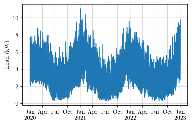
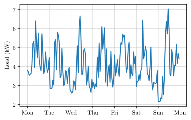
Figure 2: Hourly loads from a home in Trondheim, Norway. Top. Three-year period from 1 January 2020 to 31 December 2022. Bottom. One week in January 2022.

3.1 System parameters

We use intervals that are one hour long, so $h=1$. The hourly loads $l_{t}$ are shown in figure 2, over the full three years (top) and zoomed in to one week in January 2022 (bottom).

The system parameters are

$$P=20\,\text{kW},\quad Q=40\,\text{kWh},\quad C=20\,\text{kW},\quad D=20\,\text{kW},$$

and the efficiency parameters are

$$\eta_{s}=0.99998,\quad\eta_{c}=0.95,\quad\eta_{d}=0.95.$$

With these parameters, a complete charge or discharge of the battery will take 2 hours. The per-hour storage efficiency $\eta_{s}$ is equivalent to a $1.5\%$ monthly self-discharge rate, which is typical for lithium-ion batteries. The charging and discharging efficiencies represent a loss of $5\%$. We take the initial and final charge levels as both half full, i.e., $q_{\mathrm{init}}=q_{\mathrm{final}}=Q/2$. In some numerical experiments we will vary the storage capacity $Q$ from its nominal value $40$ kW specified above, to study the effect of cost saving versus storage capacity.

3.2 Price parameters

Figure 3 shows the day-ahead prices $\lambda_{t}^{\mathrm{da}}$ for Trondheim, Norway, expressed in Norwegian Krone (NOK) per kW, sourced from Nord Pool [45]. The top figure covers the three-year period from 1 January 2020 to 31 December 2022, while the bottom figure zooms in on a particular week in January 2022. Day-ahead prices are announced daily at 13:00 for the following day.

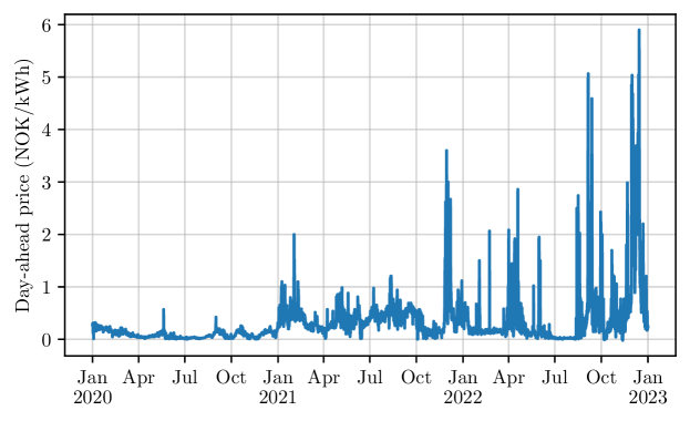
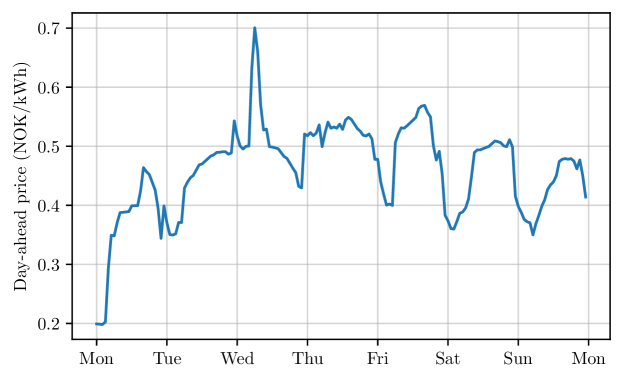
Figure 3: Day-ahead electricity prices $\lambda_{t}^{\mathrm{da}}$ for Trondheim, Norway. Top. Three-year period from 1 January 2020 to 31 December 2022. Bottom. One week in January 2022.

Figure 4 shows the time-of-use prices, which fluctuate according to the time of day and season, with distinct rates for the daytime period (6:00–22:00) and nighttime period (22:00–6:00), as well as different rates for January–March and April–December.

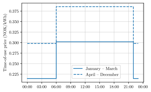
Figure 4: Time-of-use electricity prices $\lambda_{t}^{\mathrm{tou}}$ with distinct rates for day (6:00–22:00) and night (22:00–6:00) as well as for the period of January–March and April–December.

The tiered cost values for the peak power cost $\beta_{l}$ are

$$\beta_{1}=83,\quad\beta_{2}=147,\quad\beta_{3}=252,\quad\beta_{4}=371,\quad\beta_{5}=490,$$

and the corresponding thresholds $T_{l}$ are

$$T_{1}=2,\quad T_{2}=5,\quad T_{3}=10,\quad T_{4}=15,$$

with $T_{5}=P=20$. Figure 5 shows the peak power cost function.

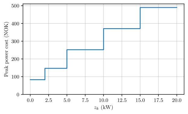
Figure 5: Peak power cost as a function of $z_{k}$, the average of the $N=3$ largest peak daily powers over a month.

3.3 Baseline

For reference we consider a baseline scenario without storage. Using load and price data from 2022, we obtain a total annual cost of $25,052$ NOK, broken down into $8,685$ NOK for the time-of-use energy charges, $13,343$ NOK for the day-ahead energy charges, and $3,024$ NOK for the peak power charges. A breakdown of the charges by month is shown in figure 6. The greatest variation in monthly cost is in the day-ahead energy charges.

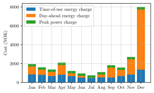
Figure 6: Monthly costs without storage for 2022, broken down into time-of-use energy charges (blue), day-ahead energy charges (orange), and peak power charges (green).

4 Prescient problem

In the prescient problem, we assume all parameters are known, including future loads and day-ahead prices. The prescient problem can be expressed as the optimization problem

$$\begin{array}[]{ll}\mbox{minimize}&h\sum_{t=1}^{T-1}(\lambda_{t}^{\mathrm{tou}}+\lambda_{t}^{\mathrm{da}})p_{t}+\sum_{k=1}^{K}\sum_{l=1}^{L}\beta_{l}s_{lk}\\ \mbox{subject to}&p_{t}+d_{t}-l_{t}-c_{t}=0,\quad t=1,\ldots,T-1\\ &q_{t+1}=\eta_{s}q_{t}+\eta_{c}c_{t}-(1/\eta_{d})d_{t},\quad t=1,\ldots,T-1\\ &q_{1}=Q/2,\quad q_{T}=Q/2\\ &0\leq q_{t}\leq Q,\quad t=1,\ldots,T\\ &0\leq p_{t}\leq P,\quad t=1,\ldots,T-1\\ &0\leq c_{t}\leq C,\quad t=1,\ldots,T-1\\ &0\leq d_{t}\leq D,\quad t=1,\ldots,T-1\\ &m_{k}=\mbox{daily max power in month $k$},\quad k=1,\ldots,K\\ &z_{k}=\psi(m_{k},N)/N,\quad k=1,\ldots,K\\ &z_{k}\leq\sum_{l=1}^{L}T_{l}s_{lk},\quad k=1,\ldots,K\\ &\sum_{l=1}^{L}s_{lk}=1,\quad k=1,\ldots,K\\ &s_{lk}\in\{0,1\},\quad l=1,\ldots,L,\quad k=1,\ldots,K\end{array}$$ (2)

with continuous variables $p\in{\mbox{\bf R}}^{T-1}$, $c\in{\mbox{\bf R}}^{T-1}$, $d\in{\mbox{\bf R}}^{T-1}$, $q\in{\mbox{\bf R}}^{T}$, and the integer variables $s_{lk}\in\{0,1\}$, for $l=1,\ldots,{L}$ and $k=1,\ldots,K$. We write out the description of $m_{k}$ in words, to simplify notation. Each entry is the maximum of 24 contiguous values of $p$, corresponding to one day. These are assembled into one vector with dimension equal to the number of days in month $k$. Our problem contains a total of around $4T$ continuous scalar variables, and $LK$ integer variables. Note that the integer variables are really selection variables, since for each month $k$, exactly one $s_{lk}$ is equal to one, with the others equal to zero. If $s_{lk}=1$, $z_{k}$ falls into the tier associated with cost $\beta_{l}$.

4.1 MILP formulation

The problem (2) is a mixed-integer convex problem (MICP). To see this, we ignore the constraints that $s_{i}\in\{0,1\}$, and recognize the objective above as linear, and most of the constraints as linear equality and inequality constraints. The subtleties are that $m_{k}$ are convex expressions (since they are the max of subsets of $p$), and $z_{k}$ are also convex expressions, since $\psi(m_{k},N)$ is a convex nondecreasing function [7, §3.2.3]. It follows that all constraints except $s_{lk}\in\{0,1\}$ are convex, so the prescient policy problem (2) is a MICP.

The two functions appearing in the problem, max and sum-largest, are each piecewise linear convex and can be represented via linear programming by various reductions. It follows that the problem (2) can be transformed to an equivalent MILP. These reductions can be done automatically by domain specific languages (DSLs) for convex optimization such as CVXPY [25]. To solve the resulting MILPs, a wide range of solvers are available, both commercial and open-source. CVXPY can interface with commercial solvers such as MOSEK [5], CPLEX [14], and GUROBI [44], as well as open-source solvers such as GLPK_MI [18], CBC [8], SCIP [12], and HiGHs [35].

4.2 CVXPY implementation

We specify and solve problem (2), for our running example, using CVXPY as outlined in the code below. We assume that vectors containing hourly loads l, time-of-use prices tou_prices, day-ahead prices da_prices, and a pandas [41] datetime index dt spanning $T-1$ time periods have been defined.

We start by defining constants and parameters in lines 4–9. We then define the optimization variables p, c, d, q, and s in lines 12–16. We then specify the following constraints: power balance (line 19), storage dynamics (line 20), initial and final charge levels (line 21), maximum storage capacity, maximum grid power, and maximum charging and discharging rates (line 22). The total energy charge, denoted as energy_cost, is defined in line 25.

In lines 28–35, we specify the constraints and the cost term related to peak power charges. For each month, we compute the vector of daily maximum powers m_k (line 30–31). We then compute the average of the N largest daily maximum powers, denoted as z_k (line 32). With this, we define the peak power charge (line 33) and add constraints to ensure that z_k does not exceed the tier thresholds, and that exactly one tier is selected per month (line 34–35).

Finally, we specify and solve the optimization problem in lines 38–39.

CVXPY code for prescient problem.

⬇

1import cvxpy as cp, numpy as np, pandas as pd

2

3# Define constants and parameters

4P, N, Q = 20, 3, 40

5q_init, q_final, C, D = Q/2, Q/2, Q/2, Q/2

6eta_s, eta_c, eta_d = 0.99998, 0.95, 0.95

7tier_costs = np.array([83, 147, 252, 371, 490])

8tier_thresholds = np.array([2, 5, 10, 15, P])

9T, K, L = len(l)+1, len(set(dt.month)), len(tier_costs)

10

11# Define variables

12p = cp.Variable(T-1, nonneg=True)

13c = cp.Variable(T-1, nonneg=True)

14d = cp.Variable(T-1, nonneg=True)

15q = cp.Variable(T, nonneg=True)

16s = cp.Variable((K, L), boolean=True)

17

18# Define constraints

19cons = [p + d - l - c == 0,

20 q[1:] == eta_s * q[:-1] + eta_c * c - (1/eta_d) * d,

21 q[0] == q_init, q[-1] == q_final,

22 q <= Q, p <= P, c <= C, d <= D]

23

24# Define energy charges

25energy_cost = cp.sum(cp.multiply(tou_prices + da_prices, p))

26

27# Define peak power charges and constraints

28peak_power_cost = 0

29for k in range(K):

30 m_k = [cp.max(p[(dt.date == day) & (dt.month == k+1)])

31 for day in pd.unique(dt[dt.month == k+1].date)]

32 z_k = cp.sum_largest(m_k, N) / N

33 peak_power_cost += cp.matmul(tier_costs, s[k, :])

34 cons += [z_k <= cp.matmul(tier_thresholds, s[k, :]),

35 cp.sum(s[k, :]) == 1]

36

37# Define problem and solve

38problem = cp.Problem(cp.Minimize(energy_cost + peak_power_cost), cons)

39problem.solve()

4.3 Running example

Computation.

We solve the prescient problem (2) using load and price data from 2022, using CVXPY with the solver Gurobi 10.0.1. After compilation by CVXPY, the problem has $35781$ continuous variables and $48$ integer variables. On a computer with Apple M1 Pro processor and $16$ GB of RAM, it takes around $3$ seconds to solve. (With the other MILP solvers mentioned above, it takes a bit longer.)

Results.

The optimal cost is $21,204$ NOK, which corresponds to savings of $3,848$ NOK (or $15.4\%$) compared to the no-storage baseline. A cost comparison with a breakdown of charges is shown in table 1. We can see that the greatest fractional savings is in the peak power charge, while the greatest savings is in the day-ahead energy charge. Figure 7 gives a detailed monthly breakdown of this annual cost, broken down into energy charges from time-of-use and day-ahead prices, and peak power charges. We can see that the greatest savings occur in the highest cost months November and December.

Table 1: Cost comparison for 2022 between no-storage baseline and prescient policy ($40\,\text{kWh}$ storage capacity). Costs are in NOK.

	Energy charge		Peak power charge	Total cost	Savings w.r.t. baseline
	TOU prices	DA prices
Baseline	$8,685$	$13,343$	$3,024$	$25,052$
Prescient	$8,374$	$11,025$	$1,805$	$21,204$	$3,848$ ($15.4\%$)

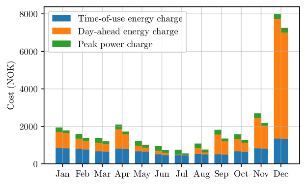
Figure 7: Monthly costs over 2022 for no-storage baseline (left) and prescient policy (right). Each broken down into time-of-use charges (blue), day-ahead charges (orange), and peak power charges (green).

Optimal power flows.

Figure 8 illustrates the prescient optimal power flows over a full year. The top left and right figures show the power drawn from the grid and the load, respectively. Without storage, the grid power profile matches the load profile. With storage, we can see that the optimal grid power profile typically peaks at a lower monthly level to minimize the peak power charge, an effect commonly referred to as peak shaving. The middle left and right figures show the charging and discharging storage power, respectively. The bottom left figure provides a view of the battery’s charge level over the full year. In the bottom right figure, we show $z_{k}$, i.e., the average of the $N=3$ largest maximum daily powers each month. We can see that the optimal tiers are tier 1 for July, tier 3 for December, and tier 2 for all other months.

Figure 9 provides a detailed view of one week in July 2022. The figures follow the same order as in Figure 8. In addition to the peak shaving effect mentioned previously, we can observe that power is often drawn from the grid during periods of lower prices, an effect commonly referred to as load shifting.

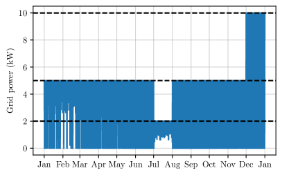
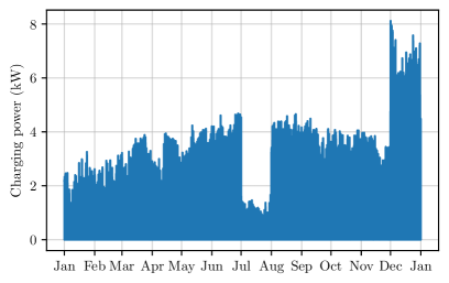
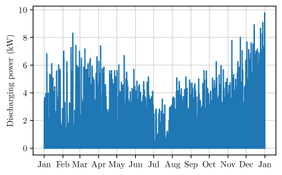
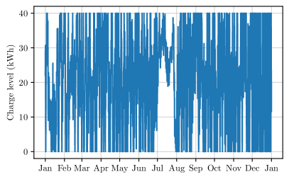
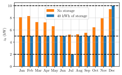
Figure 8: Optimal power flows over 2022 assuming perfect foresight, with tier thresholds shown as dashed black lines. Top left. Power drawn from the grid. Top right. Load. Middle left. Charging storage power. Middle right. Discharging storage power. Bottom left. Charge level. Bottom right. Average of the $N=3$ largest maximum daily power flows in each month, $z_{k}$, with and without storage.

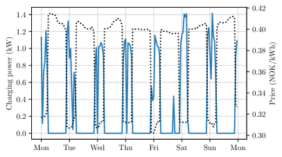
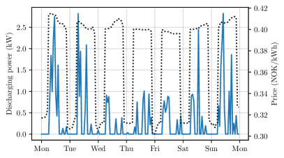
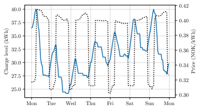
Figure 9: Optimal power flows over one week in July 2022 assuming perfect foresight, with tier thresholds shown as dashed black lines. Hourly electricity prices, $\lambda_{t}^{\mathrm{tou}}+\lambda_{t}^{\mathrm{da}}$, are shown as dotted black lines. Top left. Power drawn from the grid. Top right. Load. Middle left. Charging storage power. Middle right. Discharging storage power. Bottom. Charge level.

Savings versus storage capacity.

We solve the prescient problem for a range of values of storage capacity $Q$. Figure 10 shows the annual savings versus capacity. Without the integer constraints, this curve would be piecewise linear concave; but here we see that with these constraints, it is very close to concave. With half the nominal storage, $20$ kWh, we achieve a reduction of around $12.5\%$, around 80% of the nominal savings $15.5\%$.

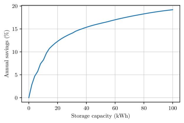
Figure 10: Annual savings versus storage capacity for 2022.

5 Model predictive control

In this section we describe a standard method, model predictive control (MPC), also known as receding horizon control (RHC), that can be used to develop a causal strategy or policy.

In each time period $t$, we consider a horizon that extends $H$ time periods into the future, $t,t+1,\ldots,t+H-1$. Given the initial state of the system, we solve an optimal power flow problem over this horizon, replacing unkown quantities by predictions or forecasts. We then execute the first power flow in that plan and repeat this process at the next time step, incorporating any new information into our forecasts. Below, we describe these steps in more detail.

Forecast.

At time $t$, we make predictions of future loads, denoted by $\hat{l}_{\tau|t}$, and day-ahead prices, denoted by $\hat{\lambda}_{\tau|t}^{\mathrm{da}}$. These predictions extend from $\tau=t,t+1,\ldots,t+H-1$. Note that all quantities at time $t$ are known, i.e., $\hat{l}_{t|t}=l_{t}$ and $\hat{\lambda}_{t|t}^{\mathrm{da}}=\lambda_{t}^{\mathrm{da}}$. (We use the hat to indicate that the quantity is an estimate.) In §6, we describe how to generate simple forecasts from historical data. In each time period, some future day-ahead prices are known, so these forecasts are perfect.

Plan.

At time $t$, we make a power flow plan over the next $H$ time periods, from $\tau=t$ to $\tau=t+H-1$. These periods span a total of $M$ months, from $j=k$ to $j=k+M-1$. To make this plan we solve problem (2), with time periods shifted from $t=1,\ldots,T$ to $\tau=t,\ldots,t+H$, month indices shifted from $k=1,\ldots,K$ to $j=k,\ldots,k+M-1$, day-ahead prices and loads replaced by their estimated values at time $t$. Moreover, the initial charge, a state variable in our MPC formulation, is set to the known value $q_{t}$.

To compute the peak power cost in the current month, we consider the $N$ largest maximum daily powers executed from the start of the month up to the current day, including the maximum power for the current day itself. These are additional state variables in the MPC formulation, which we use to compute $m_{k}$ and $z_{k}=\psi(m_{k},N)$. For the remaining months within the horizon, $m_{j}$ is computed based on the predicted power flows for each month. If a given month has less than $N$ days in our horizon, we set $N$ to the number of days in that month for the calculation of $z_{j}$.

Execute.

We implement the first power flow in the plan, i.e., the power flows corresponding to time period $t$. Note that the planned power flows from $\tau=t+1$ to $\tau=t+H-1$ are never executed. Their purpose is only to improve the choice of power flows in the first step, which we do execute.

5.1 Running example

We run MPC with planning horizon $H=720$ hours (30 days). This planning horizon straddles a maximum of two months. We have found that considering a surrogate peak power charge with $N=1$ in the MPC formulation instead of $N=3$ works better, i.e., we penalize the peak power in each month instead of the average of the $N=3$ largest peak powers in different days, which is the true peak power charge. (Of course our analysis of the cost uses the correctly computed peak power.) We use forecasts of load and day-ahead prices described in §6.

Computation.

The MPC problem can be solved using an MILP solver. But since there are only a small number of integer variables in it, we can just as well solve it globally by solving individual LPs corresponding to the possible choices of tiers for the current and next month. It takes around $0.07$ seconds to solve the MILP problem with the commercial solver Gurobi 10.0.1 and around $0.03$ seconds to solve each LP problem with the commercial solver MOSEK 10.0.40. (With the other solvers it takes a bit longer.) Note that the LP problems can be solved in parallel.

Results.

With the MPC policy (setting $N=1$), we achieve a cost of $21,564$ NOK, which corresponds to savings of $3,488$ NOK (or $13.9\%$) with respect to the no-storage baseline. This means that the MPC policy is able to recover more than $90\%$ of the cost reduction that can be achieved using perfect foresight. The MPC policy is at most $1.7\%$ suboptimal.

A cost comparison with a breakdown of charges is presented in table 2. Most of the suboptimality in MPC, when compared to the prescient policy, comes from the peak power charge. Similar to the prescient case, the greatest fractional savings is in the peak power charge, while the greatest savings is in the day-ahead energy charge. An interesting deviation is seen in the time-of-use energy charge under MPC, which is, in fact, lower than that when using perfect foresight. Figure 11 gives a detailed monthly breakdown of this annual cost, further differentiating between energy charges (calculated from time-of-use and day-ahead prices) and peak power charges.

For comparison, we also evaluate the performance of the MPC with $N=3$. This results in a cost of $21,568$ NOK, yielding savings of $3,484$ NOK (or $13.91\%$) against the no-storage baseline. The suboptimality gap in this case is $1.72\%$, which represents only a marginal increase when compared to the case with $N=1$.

Table 2: Cost comparison for 2022 between no-storage baseline, prescient policy, and MPC policy ($40\,\text{kWh}$ storage capacity). Costs are in NOK.

	Energy charge		Peak power charge	Total cost	Savings w.r.t. baseline
	TOU prices	DA prices
Baseline	$8,685$	$13,343$	$3,024$	$25,052$
Prescient	$8,374$	$11,025$	$1,805$	$21,204$	$3,848$ ($15.4\%$)
MPC	$8,236$	$11,039$	$2,289$	$21,564$	$3,488$ ($13.9\%$)

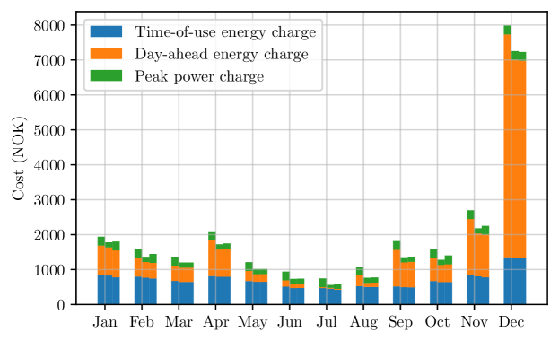
Figure 11: Monthly costs over 2022 for no-storage baseline (left), prescient policy (middle), and MPC policy (right). Each broken down into time-of-use charges (blue), day-ahead charges (orange), and peak power charges (green).

MPC power flows.

Figure 12 presents the power flows executed by the MPC policy over 2022. The top left figure shows the power drawn from the grid, while the top right figure depicts the load. The middle left and right figures show the charging and discharging storage power, respectively. We observe that the peak power using MPC exceeds that of the prescient case in several months, as can be seen in the bottom right figure, where we show the monthly $z_{k}$ values. This figure illustrates the average of the $N=3$ largest daily powers in each month, both with and without storage. The $z_{k}$ values fall into tier 2 in $7$ out of the $12$ months (from March to September) and into tier 3 the ramaining $5$ months. The bottom left figure shows the battery’s charge level over the year.

Figure 13 provides a detailed view of one week in July 2022. We observe again the load shifting and peak shaving effects of the battery. However, the peak power usage is $5\,\text{kW}$, contrasting with $2\,\text{kW}$ in the prescient case.

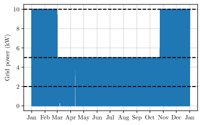
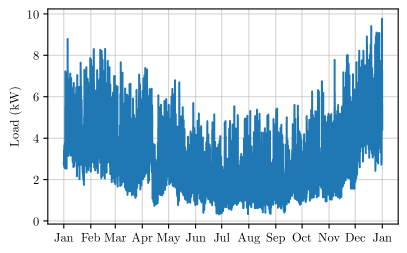
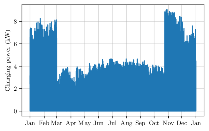
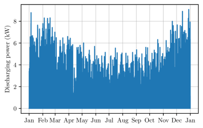
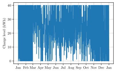
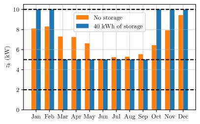
Figure 12: Power flows executed over 2022 using MPC, with tier thresholds shown as dashed black lines. Top left. Power drawn from the grid. Top right. Load. Middle left. Charging storage power. Middle right. Discharging storage power. Bottom left. Charge level. Bottom right. Average of the $N=3$ largest maximum daily power flows in each month, $z_{k}$, with and without storage.

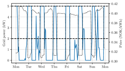
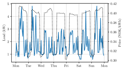
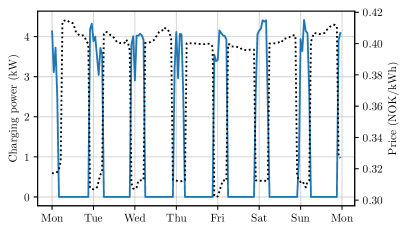
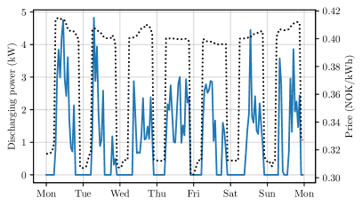
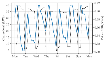
Figure 13: Power flows executed over one week in July 2022 using MPC, with tier thresholds shown as dashed black lines. Hourly electricity prices, $\lambda_{t}^{\mathrm{tou}}+\lambda_{t}^{\mathrm{da}}$, are shown as dotted black lines. Top left. Power drawn from the grid. Top right. Load. Middle left. Charging storage power. Middle right. Discharging storage power. Bottom. Charge level.

Comparison with simpler forecasts.

The MPC results in table 2 were obtained using forecasts generated from historical data using the methods outlined in §6. For comparison, we tested MPC with simpler forecasts that reduce the need for historical data. For load prediction, we assume that the load over the next $23$ hours is equal to the load from the last $23$ hours. This $24$-hour prediction (we know the current load at time $t$) is then repeated over the rest of the horizon. Therefore, we only need to store $24$ hours of load data to generate this forecast.

Day-ahead prices are disclosed daily at 13:00 for the following day, providing us with an advanced window ranging from $12$ (at 12:00) to $35$ hours (at 13:00) of known prices. We use this perfect forecast in our MPC formulation. When the MPC horizon extends beyond the period of known prices, we augment the forecast by repeating the last known value.

Using these basic forecasts and setting $N=1$, MPC achieves a cost of $21,907$ NOK, which translates to savings of $3,145$ NOK (or $12.5\%$) compared to the no-storage baseline, with a suboptimality gap of $3.3\%$. When setting $N=3$, MPC achieves a cost of $22,100$ NOK, yielding savings of $2,952$ NOK (or $11.8\%$) against the no-storage baseline. The suboptimality gap in this case is $4.2\%$. These results indicate that even with such basic forecasts, MPC is able to deliver reasonably good performance.

6 Forecasting

In this section we describe a simple method to forecast a scalar time series $x_{1},x_{2},\ldots$ using historical data, based on the methods suggested in [38, Appendix A].

6.1 The baseline-residual forecast

The baseline-residual forecast is given by

$$\hat{x}_{\tau|t}=b_{\tau}+\hat{r}_{\tau|t},$$

where $\hat{x}_{\tau|t}\in{\mbox{\bf R}}$ is the prediction of quantity $x$ at time $\tau$ made at time $t<\tau$. The forecast $\hat{x}_{\tau|t}$ consists of two components: a seasonal baseline $b_{\tau}$ that captures periodically repeating patterns (e.g., diurnal, weekly, and seasonal variations), and an autoregressive residual term $\hat{r}_{\tau|t}$ that accounts for short-term deviations from the baseline based on recent past observations. The baseline prediction depends only on the time $\tau$ of the predicted quantity, and not the time $t$ at which the prediction is made. The forecast of the residual at time $\tau$, on the other hand, depends on $t$, the time at which the forecast is made. We describe below how to compute each of these components.

Multi-sine baseline forecast.

A simple model for the baseline is a sum of $K$ sinusoids,

$$b_{t}=\beta_{0}+\sum_{k=1}^{K}\alpha_{k}\sin\left(\frac{2\pi t}{P_{k}}\right)+\beta_{k}\cos\left(\frac{2\pi t}{P_{k}}\right),$$

where $\alpha_{k}$ and $\beta_{k}$ are the coefficients and $P_{k}$ are the periods. In the usual case of Fourier series, the periods have the form $P_{k}=P/k$, where $P$ is the fundamental period. But here we will introduce terms that model seasonal variation, weekly variation, and daily or diurnal variation.

To fit the vector of $2K+1$ coefficients $\beta_{0},\alpha_{1},\beta_{1},\ldots,\alpha_{K},\beta_{K}$ to some historical training data $x_{1},\ldots,x_{T}$, we use a pinball or quantile loss function with ridge regularization. (The pinball loss is robust, and allows us to create conservative forecasts that are more likely to overestimate or underestimate the true value, depending on the choice of a parameter.) The pinball loss function for quantile $\eta\in[0,1]$ is defined as

$$L_{\eta}(u)=\max\{(1-\eta)u,\eta u\}=(\eta-1/2)|u|+(1/2)u.$$

To find the coefficients we minimize

$$\sum_{t=1}^{T}L_{\eta}(b_{t}-x_{t})+\lambda\sum_{k=1}^{K}\nu_{k}(\alpha_{k}^{2}+\beta_{k}^{2}),$$

where $\lambda>0$ is the regularization parameter, and $\nu_{k}>0$ are parameters set to the square of the harmonics (e.g., 1, 4, 9, 16 for the 1st, 2nd, 3rd, and 4th harmonics, respectively) across all variation types, including daily, weekly, and annual. This choice implies a higher penalty for higher harmonics, thereby dampening their influence in the model. This is a convex problem and readily solved. Good values for $\eta$ and $\lambda$ can be chosen via out-of-sample or cross-validation [6, §7.10], [34, §13.2].

Auto-regressive residual forecast.

Once we have the baseline forecast, we substract it from our historical data to obtain the sequence of historical residuals, $r_{t}=x_{t}-b_{t}$, $t=1,\ldots,T$. We fit an auto-regressive (AR) model to predict the residual $r_{t}$ over the next $L$ time periods, given the previous $M$. The residual AR model has the form

$$(\hat{r}_{t+1|t},\ldots,\hat{r}_{t+L|t})=\Gamma(r_{t-M+1},\ldots,r_{t}),$$

where $\Gamma\in{\mbox{\bf R}}^{L\times M}$ is the AR parameter matrix. To fit $\Gamma$ we minimize

$$\sum_{t=1}^{T}\sum_{\tau=t+1}^{t+L}L_{\eta}(\hat{r}_{\tau|t}-r_{\tau})+\lambda\|\Gamma\|_{F}^{2},$$

where $\|\cdot\|_{F}$ denotes the Frobenius norm, i.e., square root of the sum of the squares of the entries, and $\lambda>0$ is the regularization parameter. Good values for $\eta$ and $\lambda$ can be chosen via out-of-sample or cross-validation.

6.2 Running example

Load forecasting.

We use the baseline-residual forecast describe above to predict the load. In the baseline component we model diurnal (24 hours), weekly, and seasonal (annual) periodicities, with $4$ harmonics each. Therefore, we choose periods

$$\begin{array}[]{l}P_{1}=24/1,~{}P_{2}=24/2,~{}P_{3}=24/3,~{}P_{4}=24/4,\\ P_{5}=168/1,~{}P_{6}=168/2,~{}P_{7}=168/3,~{}P_{8}=168/4,\\ P_{9}=8760/1,~{}P_{10}=8760/2,~{}P_{11}=8760/3,~{}P_{12}=8760/4.\end{array}$$

We fit these 25 parameters on historical hourly data spanning two years (2020-2021). Figure 14 shows a comparison of the load and the baseline prediction for one week in both January (top) and June (bottom) of 2022.

In addition to the baseline, we fit an auto-regressive (AR) model to predict the residuals over the next $23$ hours, given the previous $24$. We fit the $23\times 24$ matrix of model parameters $\Gamma$ using quantile regression with (weighted) ridge regularization on historical hourly data collected over the same two-year period (2020-2021). A comparison between a baseline forecast with and without auto-regressive residual component is shown in figure 15 for a test day in May 2022.

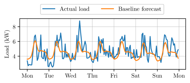
Figure 14: Seasonal baseline forecast for $\eta=0.5$ (orange) and actual load (blue). Top. One week in January 2022. Bottom. One week in June 2022.

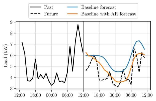
Figure 15: Comparison of forecasts for a test day in May 2022. The vertical line indicates the hour the forecast is made. The solid black line represents the load in the last 24 hours, while the dashed black line represents the load in the next 23 hours. The blue line represents a forecast that uses only a seasonal baseline model and the orange line corresponds to a forecast with both a seasonal baseline and an auto-regressive residual component.

Forecasting day-ahead prices.

We generate a baseline-residual forecast as before. This forecast is used to extend the window of known prices, that ranges between $12$ (at 12:00) to $35$ hours (at 13:00). Figure 16 shows a comparison of day-ahead prices and the baseline prediction for one week in both January (top) and June (bottom) of 2022. A comparison between a baseline forecast with and without auto-regressive residual component is shown in figure 17 for a test day in May 2022.

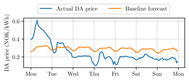
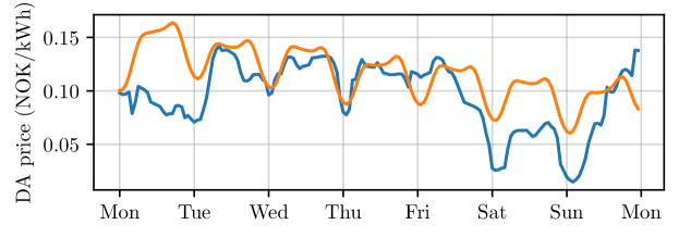
Figure 16: Seasonal baseline forecast (orange) and actual day-ahead prices (blue). Top. One week in January 2022. Bottom. One week in June 2022.

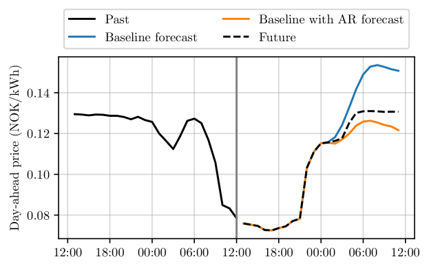
Figure 17: Comparison of forecasts for a test day in May 2022. The vertical line indicates the hour the forecast is made. The solid black line represents day-ahead prices in the last 24 hours, while the dashed black line represents day-ahead prices in the next 23 hours. The blue line represents a forecast that uses only a seasonal baseline model and the orange line corresponds to a forecast with both a seasonal baseline and an auto-regressive residual component.

7 Conclusions

We propose an MPC policy to manage a storage device in a grid-connected home, with the objective of minimizing the cost of power consumption. This cost includes a time-varying usage price and a tiered peak power charge, which depends on the average of the largest $N$ daily powers over a month. Numerical experiments on real data from a home in Trondheim, Norway, equipped with a storage capacity of $40\,\text{kWh}$, show that the MPC achieves annual savings of $13.9\%$ compared to a no-storage baseline, with a cost only $1.7\%$ higher than the optimal prescient performance bound.

References

- [1] Richard Bellman, Irving Glicksberg and Oliver Gross “On the optimal inventory equation” In Management Science 2.1 INFORMS, 1955, pp. 83–104
- [2] Sandford Berg and Andreas Savvides “The theory of maximum kW demand charges for electricity” In Energy economics 5.4 Elsevier, 1983, pp. 258–266
- [3] Stephen Henderson “The economics of electricity demand charges” In The Energy Journal 4.Special Issue International Association for Energy Economics, 1983
- [4] J. Alt, M. Anderson and R. Jungst “Assessment of utility side cost savings from battery energy storage” In IEEE Transactions on Power Systems 12.3 IEEE, 1997, pp. 1112–1120
- [5] Erling Andersen and Knud Andersen “The MOSEK interior point optimizer for linear programming: an implementation of the homogeneous algorithm” In High performance optimization Springer, 2000, pp. 197–232
- [6] Trevor Hastie, Robert Tibshirani and Jerome Friedman “The elements of statistical learning. Springer series in statistics” In New York, NY, USA, 2001
- [7] Stephen Boyd and Lieven Vandenberghe “Convex optimization” Cambridge university press, 2004
- [8] John Forrest and Robin Lougee-Heimer “CBC user guide” In Emerging theory, methods, and applications INFORMS, 2005, pp. 257–277
- [9] Alexdandre Oudalov, Daniel Chartouni, Christian Ohler and Gerhard Linhofer “Value analysis of battery energy storage applications in power systems” In 2006 IEEE PES Power Systems Conference and Exposition, 2006, pp. 2206–2211 IEEE
- [10] Frank Wolak “Residential customer response to real-time pricing: The anaheim critical peak pricing experiment”, 2007
- [11] Alaa Mohd et al. “Challenges in integrating distributed energy storage systems into future smart grid” In 2008 IEEE international symposium on industrial electronics, 2008, pp. 1627–1632 IEEE
- [12] Tobias Achterberg “SCIP: solving constraint integer programs” In Mathematical Programming Computation 1 Springer, 2009, pp. 1–41
- [13] Hassan Farhangi “The path of the smart grid” In IEEE power and energy magazine 8.1 IEEE, 2009, pp. 18–28
- [14] “User’s manual for CPLEX V12.1” In IBM 46.53, 2009, pp. 157
- [15] Bruce Dunn, Haresh Kamath and Jean-Marie Tarascon “Electrical energy storage for the grid: a battery of choices” In Science 334.6058 American Association for the Advancement of Science, 2011, pp. 928–935
- [16] Corey White and Max Zhang “Using vehicle-to-grid technology for frequency regulation and peak-load reduction” In Journal of Power Sources 196.8 Elsevier, 2011, pp. 3972–3980
- [17] Wesley Cole, Thomas Edgar and Atila Novoselac “Use of model predictive control to enhance the flexibility of thermal energy storage cooling systems” In 2012 American Control Conference (ACC), 2012, pp. 2788–2793 IEEE
- [18] Free Software Foundation “GLPK - GNU Linear Programming Kit”, https://www.gnu.org/software/glpk/, 2012
- [19] Jingran Ma, Joe Qin, Timothy Salsbury and Peng Xu “Demand reduction in building energy systems based on economic model predictive control” In Chemical Engineering Science 67.1 Elsevier, 2012, pp. 92–100
- [20] Sean Ong and Ryan McKeel “National utility rate database”, 2012
- [21] Matt Kraning, Eric Chu, Javad Lavaei and Stephen Boyd “Dynamic network energy management via proximal message passing” In Foundations and Trends® in Optimization 1.2 Now Publishers, Inc., 2013, pp. 73–126
- [22] Lukas Sigrist, Enrique Lobato and Luis Rouco “Energy storage systems providing primary reserve and peak shaving in small isolated power systems: An economic assessment” In International Journal of Electrical Power & Energy Systems 53 Elsevier, 2013, pp. 675–683
- [23] Sambuddha Chakrabarti et al. “Security constrained optimal power flow via proximal message passing” In 2014 Clemson university power systems conference, 2014, pp. 1–8 IEEE
- [24] T. Shear “Today in energy: February archive” In US Energy Information Administration (EIA), Independent statistics & Analysis, 2014
- [25] Steven Diamond and Stephen Boyd “CVXPY: A Python-embedded modeling language for convex optimization” In Journal of Machine Learning Research 17.83, 2016, pp. 1–5
- [26] Alexandre Lucas and Stamatios Chondrogiannis “Smart grid energy storage controller for frequency regulation and peak shaving, using a vanadium redox flow battery” In International Journal of Electrical Power & Energy Systems 80 Elsevier, 2016, pp. 26–36
- [27] Norwegian Water Resources and Energy Directorate “Tariff reform for a smarter grid”, 2016 URL: https://publikasjoner.nve.no/rapport/2016/rapport2016_62.pdf
- [28] Rafael Sebastián “Application of a battery energy storage for frequency regulation and peak shaving in a wind diesel power system” In IET Generation, Transmission & Distribution 10.3 Wiley Online Library, 2016, pp. 764–770
- [29] Paul Simshauser “Distribution network prices and solar PV: Resolving rate instability and wealth transfers through demand tariffs” In Energy Economics 54 Elsevier, 2016, pp. 108–122
- [30] Morgan Jones and Matthew Peet “Solving dynamic programming with supremum terms in the objective and application to optimal battery scheduling for electricity consumers subject to demand charges” In 2017 IEEE 56th Annual Conference on Decision and Control (CDC), 2017, pp. 1323–1329 IEEE
- [31] Joyce McLaren, Pieter Gagnon and Seth Mullendore “Identifying potential markets for behind-the-meter battery energy storage: A survey of US demand charges”, 2017
- [32] Robert Passey, Navid Haghdadi, Anna Bruce and Iain MacGill “Designing more cost reflective electricity network tariffs with demand charges” In Energy Policy 109 Elsevier, 2017, pp. 642–649
- [33] Matt Wytock, Nicholas Moehle and Stephen Boyd “Dynamic energy management with scenario-based robust MPC” In 2017 American Control Conference (ACC), 2017, pp. 2042–2047 IEEE
- [34] Stephen Boyd and Lieven Vandenberghe “Introduction to applied linear algebra: vectors, matrices, and least squares” Cambridge university press, 2018
- [35] Qi Huangfu and Julian Hall “Parallelizing the dual revised simplex method” In Mathematical Programming Computation 10.1 Springer, 2018, pp. 119–142
- [36] Ranjeet Kumar et al. “A stochastic model predictive control framework for stationary battery systems” In IEEE Transactions on Power Systems 33.4 IEEE, 2018, pp. 4397–4406
- [37] Moira Nicolson, Michael Fell and Gesche Huebner “Consumer demand for time of use electricity tariffs: A systematized review of the empirical evidence” In Renewable and Sustainable Energy Reviews 97 Elsevier, 2018, pp. 276–289
- [38] Nicholas Moehle, Enzo Busseti, Stephen Boyd and Matt Wytock “Dynamic energy management” In Large Scale Optimization in Supply Chains and Smart Manufacturing: Theory and Applications Springer, 2019, pp. 69–126
- [39] Michael Risbeck and James Rawlings “Economic model predictive control for time-varying cost and peak demand charge optimization” In IEEE Transactions on Automatic Control 65.7 IEEE, 2019, pp. 2957–2968
- [40] Morgan Jones and Matthew Peet “Extensions of the dynamic programming framework: Battery scheduling, demand charges, and renewable integration” In IEEE Transactions on Automatic Control 66.4 IEEE, 2020, pp. 1602–1617
- [41] The pandas development team “pandas-dev/pandas: Pandas” Zenodo, 2020 DOI: 10.5281/zenodo.3509134
- [42] Wenqi Cai, Hossein Esfahani, Arash Kordabad and Sébastien Gros “Optimal management of the peak power penalty for smart grids using MPC-based reinforcement learning” In 2021 60th IEEE Conference on Decision and Control (CDC), 2021, pp. 6365–6370 IEEE
- [43] Wenqi Cai, Arash Kordabad and Sébastien Gros “Energy management in residential microgrid using model predictive control-based reinforcement learning and Shapley value” In Engineering Applications of Artificial Intelligence 119 Elsevier, 2023, pp. 105793
- [44] Gurobi Optimization, LLC “Gurobi Optimizer Reference Manual”, 2023 URL: https://www.gurobi.com
- [45] Nord Pool “Nord Pool: Power Market Operations”, 2023 URL: https://www.nordpoolgroup.com/