JWST’s PEARLS: Transients in the MACS J0416.12403 Field
Abstract
With its unprecedented sensitivity and spatial resolution, the James Webb Space Telescope (JWST) has opened a new window for time-domain discoveries in the infrared. Here we report observations in the only field that has received four epochs (spanning 126 days) of JWST NIRCam observations in Cycle 1. This field is towards MACS J0416.12403, which is a rich galaxy cluster at redshift and is one of the Hubble Frontier Fields. We have discovered 14 transients from these data. Twelve of these transients happened in three galaxies (with , 1.01, and 2.091) crossing a lensing caustic of the cluster,and these transients are highly magnified by gravitational lensing. These 12 transients are likely of similar nature to those previously reported based on the Hubble Space Telescope (HST) data in this field, i.e., individual stars in the highly magnified arcs. However, these twelve could not have been found by HST because they are too red and too faint. The other two transients are associated with background galaxies ( and 0.7093) that are only moderately magnified, and they are likely supernovae. They indicate a de-magnified supernova surface density, when monitored at a time cadence of a few months to a 3–4 m survey limit of AB mag, of 0.5 arcmin-2 integrated to . This survey depth is beyond the capability of HST but can be easily reached by JWST.
1 Introduction
New capabilities in multi-messenger and time-domain astronomy will open outstanding vistas for discovery, as highlighted, for example, in the Decadal Survey on Astronomy and Astrophysics 2020 (Astro2020) 111https://nap.nationalacademies.org/resource/26141/interactive/. A core challenge is in localizing sources on the sky and in redshift, with the primary technique being searches for electromagnetic counterparts, which calls for observatories with the best flux sensitivity and angular resolution possible.
Until recently, one of the leading observatories for this purpose was the Hubble Space Telescope (HST), which had many successes. For example, it has found high-redshift supernovae, especially those of type Ia, which constrain cosmological models. In many cases, these observations were integrated with large, general-purpose extragalactic surveys (e.g., Riess et al., 2004; Amanullah et al., 2010; Suzuki et al., 2012; Riess et al., 2018). Observations of high-redshift clusters have been important for increasing yields (e.g., Dawson et al., 2009; Hayden et al., 2021), while observations of low-redshift clusters have led to the first discovery of a supernova that is gravitationally lensed into multiple images (Kelly et al., 2015, 2016). The light curves of such supernovae, and in particular the time delay between images, provide a new route to measure the Hubble–Lemaître constant (Vega-Ferrero et al., 2018; Grillo et al., 2018, 2020; Kelly et al., 2023a, b). For another example, a novel type of transient phenomena—caustic-crossing transients—has been identified through HST observations (Kelly et al., 2018; Rodney et al., 2018; Chen et al., 2019; Kaurov et al., 2019). These are individual stars in highly magnified background galaxies lying very close to the critical curve of the lensing cluster, which are further magnified— temporarily—by intracluster stars that act as microlenses. These transients have provided a completely unexpected method to study individual stars at cosmological distances.
The advent of the James Webb Space Telescope (JWST) has brought dramatically better opportunities because of its more than an order of magnitude sensitivity increase relative to HST. The Prime Extragalactic Areas for Reionization and Lensing Science program (PEARLS; Windhorst et al., 2023), one of the programs under the JWST Interdisciplinary Scientists’ Guaranteed Time Observations (GTO), has a major time-domain science component. One of its fields is MACS J0416.12403 (hereafter M0416), which is a lensing cluster at and one of the Hubble Frontier Fields (HFF: Lotz et al., 2017). The redshift of M0416 as a whole is still uncertain at the level of , mainly because this is a merging cluster whose sub-components might have large peculiar motions. Spectroscopic campaigns on this cluster are described by Balestra et al. (2016); Caminha et al. (2017); Vanzella et al. (2021); Bergamini et al. (2021). We adopt as the fiducial redshift of this cluster. HST has previously revealed several caustic-crossing transients near two caustic-straddling arcs in M0416. Rodney et al. (2018) discovered two fast transients in an arc identified at (Caminha et al., 2017; Rodney et al., 2018), which was nicknamed “Spock” by the authors. The transient sources themselves are consistent with being supergiant stars with temperatures between K and K residing in the strongly lensed galaxy that constitutes the Spock arc (Diego et al., 2023a). Chen et al. (2019) and Kaurov et al. (2019) found a transient of similar nature in another arc identified at (Hoag et al., 2016; Caminha et al., 2017), which is named “Warhol.” In addition, the ultra-deep, UV-to-visible HST program “Flashlights” detected two high-significance caustic transients in the Spock arc and four in the Warhol arc (Kelly et al., 2022). Highly lensed regions such as these are expected to produce caustic transients continually.
To take advantage of opportunities enabled by JWST, PEARLS incorporated three epochs of NIRCam observations of M0416. We expected these data to be particularly powerful for detecting red supergiant stars at because red supergiants are bright at m. The design was also motivated by the possibility of detecting individual Population III stars through caustic transits at (Windhorst et al., 2018). Another JWST GTO program, the CAnadian NIRISS Unbiased Cluster Survey (CANUCS; Willott et al., 2022), also observed M0416 with NIRCam in a separate epoch. All these data have been taken, making M0416 the only field in JWST Cycle 1 that has four epochs of NIRCam observations. This makes M0416 the best region in the sky to date for studying infrared transients.
This paper reports a transient search using the unique 4-epoch data. The search has gone beyond the aforementioned two arcs, as we also intend to assess the general infrared transient rate in less magnified regions at depths that have never been probed before. This paper is the first in a series on this subject and presents an overview of the transients found in this field. The paper is organized as follows. The NIRCam observations and data are described in Section 2. The transient search is detailed in Section 3. Section 4 discusses the transient, and Section 5 summarizes results. All magnitudes are in the AB system, and all coordinates are in the ICRS frame (equinox 2000).
2 Observations and Data
The four epochs of NIRCam observations all used the same eight bands, namely, F090W, F115W, F150W, and F200W in the “short wavelength” (SW) channel and F277W, F356W, F410M, and F444W in the “long wavelength” (LW) channel. The native NIRCam pixel scales are 0031 pix-1 in the SW channel and 0063 pix-1 in the LW channel. As the SW channel is made up of four detectors, the observations used the INTRAMODULEBOX dithers to cover the gaps. The PEARLS observations adopted the MEDIUM8 readout pattern with “up-the-ramp” fitting to determine the count rate, while those of CANUCS used a combination of the SHALLOW4 and DEEP8 patterns. The total exposure times, dates of observation, and 5 depths of these observations are summarized in Table 1.
| Epoch | Filter | Exptime | Depth |
|---|---|---|---|
| Start UT | (s) | 5 | |
| Ep1 | F090W | 3779.343 | 28.45 |
| 2022 Oct 7 08:06:05 | F115W | 3779.343 | 28.48 |
| (0.0 days) | F150W | 2920.401 | 28.48 |
| () | F200W | 2920.401 | 28.69 |
| F277W | 2920.401 | 29.83 | |
| F356W | 2920.401 | 29.91 | |
| F410M | 3779.343 | 29.38 | |
| F444W | 3779.343 | 29.58 | |
| Ep2 | F090W | 3779.343 | 28.49 |
| 2022 Dec 29 16:00:36 | F115W | 3779.343 | 28.51 |
| (83.4 days) | F150W | 2920.401 | 28.51 |
| () | F200W | 2920.401 | 28.72 |
| F277W | 2920.401 | 29.88 | |
| F356W | 2920.401 | 29.93 | |
| F410M | 3779.343 | 29.39 | |
| F444W | 3779.343 | 29.59 | |
| Ec | F090W | 6399.115 | 28.63 |
| 2023 Jan 11 20:24:42 | F115W | 6399.115 | 28.64 |
| (96.7 days) | F150W | 6399.115 | 28.82 |
| () | F200W | 6399.115 | 29.02 |
| F277W | 6399.115 | 30.14 | |
| F356W | 6399.115 | 30.19 | |
| F410M | 6399.115 | 29.50 | |
| F444W | 6399.115 | 29.70 | |
| Ep3 | F090W | 3779.343 | 28.48 |
| 2023 Feb 10 09:12:32 | F115W | 3349.872 | 28.41 |
| (126.1 days) | F150W | 2920.401 | 28.49 |
| () | F200W | 2920.401 | 28.69 |
| F277W | 2920.401 | 29.84 | |
| F356W | 2920.401 | 29.86 | |
| F410M | 3349.872 | 29.21 | |
| F444W | 3779.343 | 29.47 |
NIRCam has two nearly identical modules (“A” and “B”) that subtend two adjacent, square fields. As the spatial orientations of the JWST instruments vary in time on an annual basis, these two fields cannot both be on the same region in the sky within a year. For this reason, all four epochs of NIRCam observations were designed to center the B module on the cluster, leaving the A module mapping different regions in the flanking area. This transient study uses only the module B data because only these are spatially overlapped.
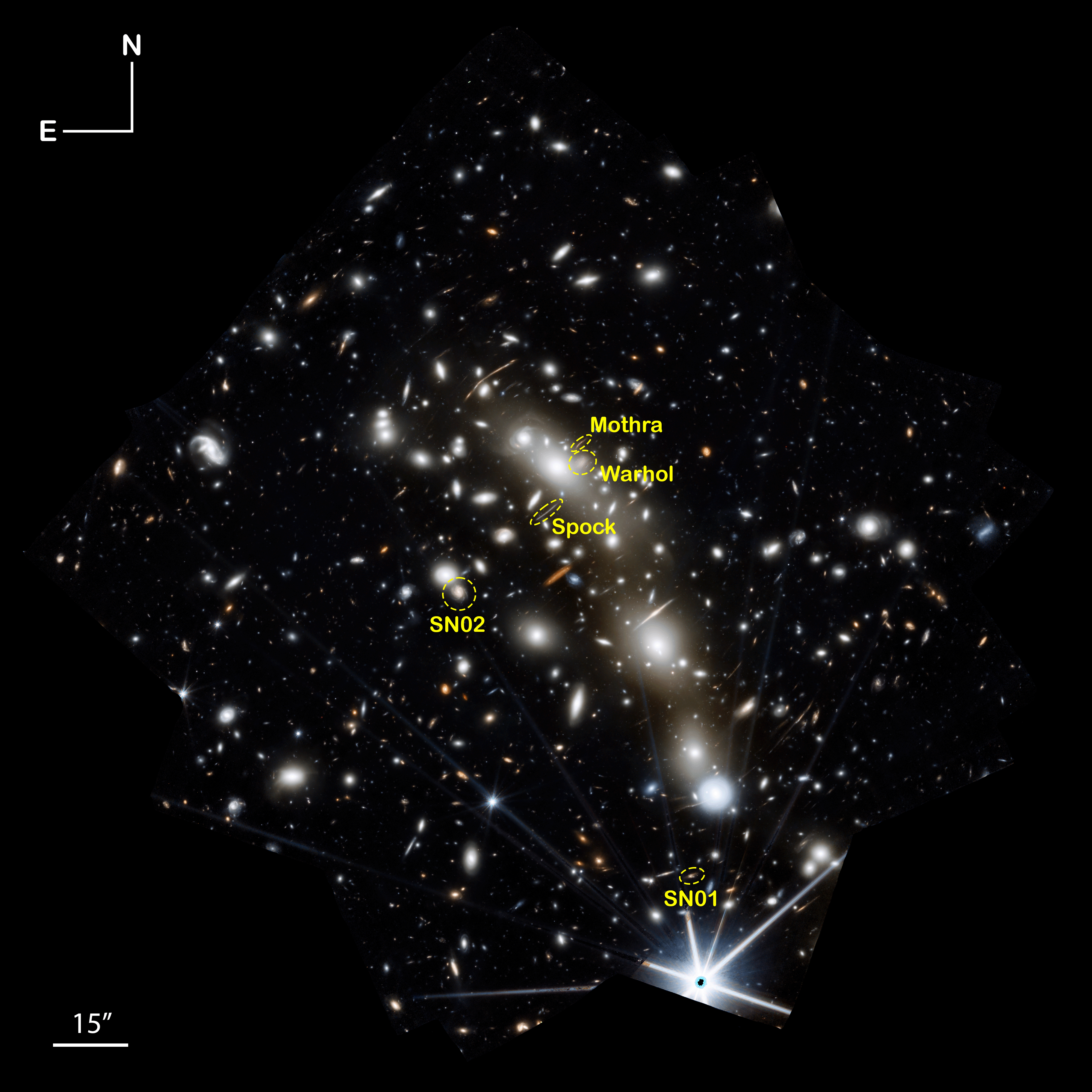
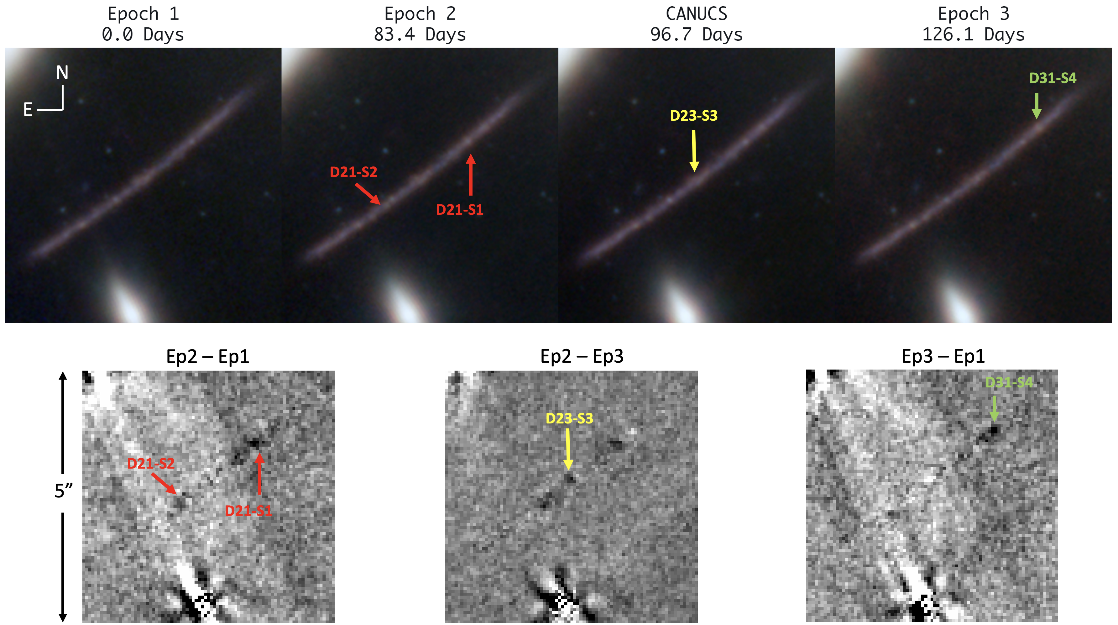
The data were retrieved from the Mikulski Archive for Space Telescopes (MAST). Reduction started from the so-called Stage 1 “uncal” products, which are the single exposures from the standard JWST data reduction pipeline (Bushouse et al., 2023) after Level 1b processing. We further processed these products using the version 1.9.4 pipeline in the context of jwst_1063.pmap. A few changes and augmentations were made to the pipeline to improve the reduction quality; most importantly, these included enabling the use of an external reference catalog for image alignment and implementing a better background estimate for the final stacking. The astrometry of each single exposure was calibrated using the public HFF products 222https://archive.stsci.edu/prepds/frontier/macs0416.html. These single images were projected onto the same grid and were stacked in each band and in each epoch. We produced two versions of stacks, one at the pixel scale of 006 (hereafter the “60mas” version) and the other at the scale of 003 (the “30mas” version), to best match the native pixel scales in the LW and the SW channels, respectively. The mosaics are in surface brightness units of MJy sr-1. The AB magnitude zeropoints are 26.581 and 28.087 for the 60mas and the 30mas stacks, respectively. Figure 1 shows a composite color image using the data from all four epochs. For convenience, we refer to the three epochs from the PEARLS program as Ep1, Ep2, and Ep3, respectively, where “p” stands for “PEARLS.” The epoch from the CANUCS program, which was between Ep2 and Ep3, is referred to as Ec (“c” for “CANUCS”).
3 Transient Discoveries
3.1 Search method
The search for transients was done in the usual way by detecting positive peaks on difference images between epochs. Thanks to the excellent image alignment and stable image quality, we were able to form the difference images by direct subtraction, for which we used the 60mas images. Due to the intense human labor in the visual inspection step (see below), this work is limited to these pairs of difference images: Ep1 Ep2 for the search of decaying sources in Ep1, Ep2 Ep1 for new sources appearing in Ep2, and Ep3 Ep1 for new sources appearing in Ep3. Ec was not used to initiate transient searches, as it was only 13.3 days after Ep2; however, it was used when studying the light curves of the identified transients. When building a difference image, its “root mean square” (RMS) map was also constructed by adding the RMS maps of the parent images in quadrature. As compared to the SW images, the LW images are less affected by defects and therefore their difference images are cosmetically cleaner. We used the F356W band as the basis of our search because its data are the deepest.
The initial transient search was to run SExtractor (Bertin & Arnouts, 1996) on the 60mas F356W difference images. The RMS maps were used in the process to estimate the signal-to-noise ratios (S/N) of the peaks in the difference images. Only the peaks that have were further considered. This left thousands of peaks in each difference image, which were then visually inspected. Not surprisingly, the vast majority of these peaks are not transient objects but are residuals caused by imperfect subtraction of bright stars and galaxies for two reasons: (1) the values of the pixels occupied by bright objects fluctuate over different epochs because of Poisson noise, which often results in positive peaks accompanied by negative peaks in a difference image; (2) the position angle of the point spread function (PSF) is different in different epochs owing to the different field orientations. This leads to spurious sources around bright objects that appear in different positions in different epochs.
After the initial visual inspection, only a few tens of transient candidates survived. To ensure their reliability, we further required that the selected transients should be detected at in the difference image of at least one more band in addition to F356W. Applying this requirement gave a total of 14 robust transients.
3.2 Descriptions of the transients and their photometry
Our sample includes seven transients in the Warhol region, four in the Spock region, one in yet another arc, and two in other regions. Their locations are indicated in Figure 1. These objects and their photometry are described below. Their magnification factors based on the lens model of Bergamini et al. (2023, adopting their 68% confidence level intervals) are also quoted along with the photometry.
In most cases, these sources are embedded in a highly non-uniform background and/or are affected by contamination from nearby objects, and PSF fitting had to be used to obtain reliable photometry. For this purpose, the 30mas images are more appropriate. To be consistent, we used PSF fitting for all objects on the 30mas images, and the detailed process is explained in the Appendix.
| R.A. | Decl. | Epoch | F090W | F115W | F150W | F200W | F277W | F356W | F410M | F444W | ||
| D21-W1 | 64.03695 | 24.06725 | Ep1 | 29.74±0.44 | 28.89±0.13 | 28.15±0.06 | 27.90±0.05 | 27.65±0.07 | 27.97±0.11 | 28.05±0.12 | 28.46±0.13 | 26.6 |
| Ep2 | 29.41±0.19 | 28.68±0.10 | 27.92±0.05 | 27.34±0.04 | 27.10±0.05 | 27.19±0.05 | 27.42±0.06 | 27.56±0.06 | ||||
| Ec | 29.09±0.22 | 28.96±0.12 | 28.28±0.06 | 27.78±0.04 | 27.61±0.06 | 27.65±0.06 | 27.79±0.07 | 28.08±0.08 | ||||
| Ep3 | 29.53±0.34 | 29.36±0.35 | 29.03±0.14 | 29.00±0.16 | 29.10±0.30 | 29.93* | 29.51* | 29.73* | ||||
| D21-W2 | 64.03674 | 24.06725 | Ep2 | 29.43±0.21 | 29.28 | 28.88±0.16 | 28.99±0.17 | 28.37±0.10 | 28.11±0.09 | 28.08±0.11 | 28.83±0.15 | 904.2 |
| Ec | 29.26±0.17 | 29.07±0.15 | 29.21±0.20 | 29.49±0.25 | 28.53±0.11 | 28.40±0.12 | 28.25±0.15 | 28.78±0.18 | ||||
| Ep3 | 28.33±0.08 | 28.31±0.08 | 28.55±0.11 | 28.89±0.16 | 29.19±0.23 | 28.67±0.16 | 28.72±0.20 | 29.09±0.21 | ||||
| D21-W3 | 64.03665 | 24.06728 | Ep2 | 29.31 | 29.28 | 29.72±0.32 | 28.88±0.14 | 28.67±0.16 | 28.42±0.12 | 28.69±0.26 | 29.10±0.23 | 331.3 |
| Ec | 29.40 | 29.38 | 30.13±0.46 | 29.78±0.33 | 29.09±0.23 | 28.66±0.14 | 28.59±0.21 | 28.77±0.17 | ||||
| Dc2-W4 | 64.03655 | 24.06731 | Ec | 28.89* | 28.87* | 29.00±0.19 | 28.18±0.11 | 27.38±0.07 | 27.04±0.06 | 27.28±0.06 | 27.36±0.07 | 1188.6 |
| D31-W5 | 64.03668 | 24.06732 | Ep3 | 29.32 | 29.29 | 29.24 | 29.28±0.22 | 28.75±0.18 | 28.62±0.16 | 28.99±0.31 | 29.62±0.39 | 83.0 |
| D31-W6 | 64.03654 | 24.06744 | Ep3 | 29.32 | 29.29 | 29.13±0.17 | 28.56±0.09 | 28.32±0.13 | 28.16±0.10 | 28.17±0.16 | 28.07±0.11 | 62.8 |
| D31-W7 | 64.03650 | 24.06736 | Ep3 | 29.32 | 29.86±0.34 | 29.71±0.30 | 28.78±0.16 | 28.50±0.15 | 28.31±0.12 | 28.64±0.20 | 28.77±0.18 | 365.9 |
3.2.1 Transients in the Warhol region
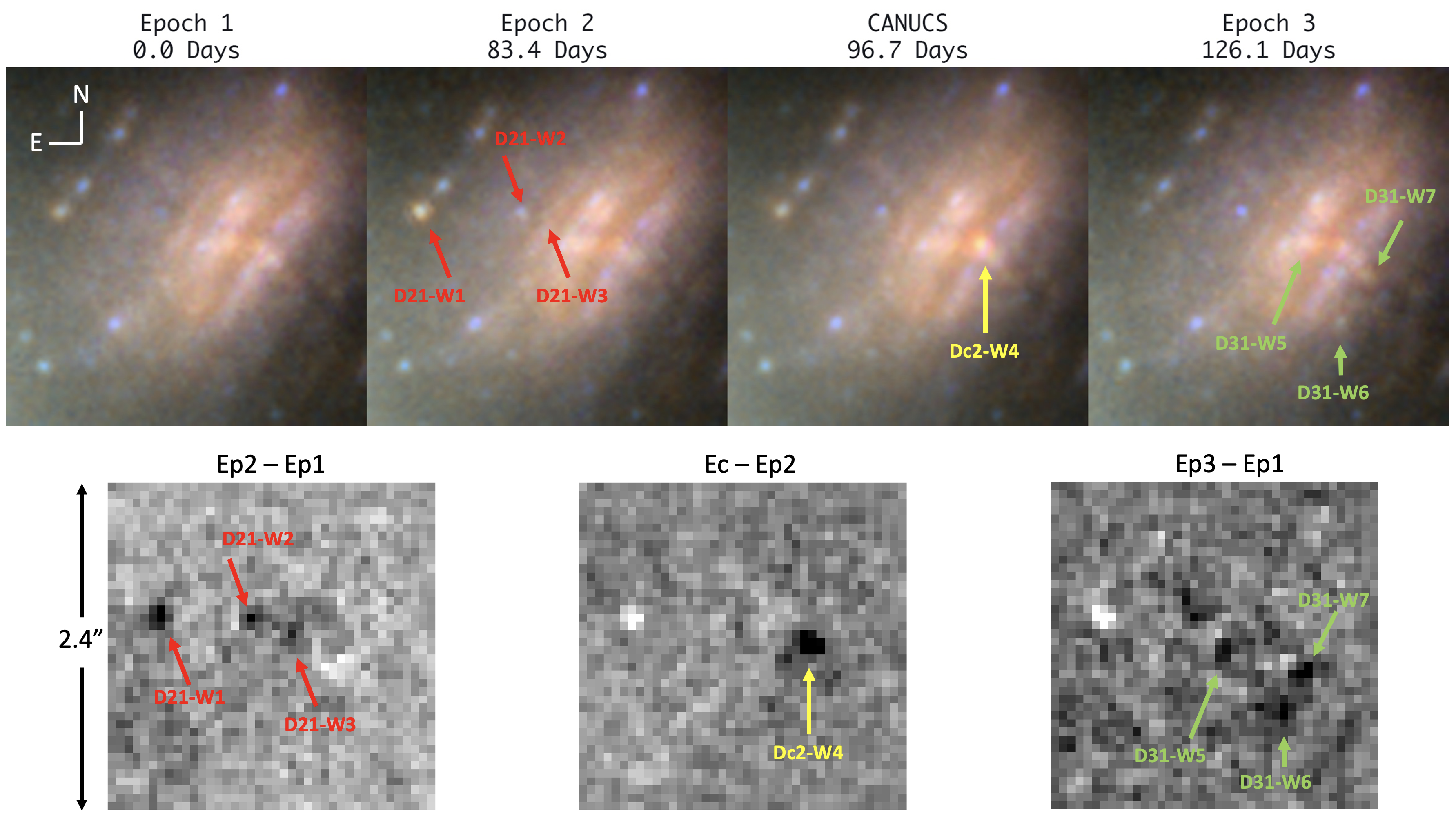
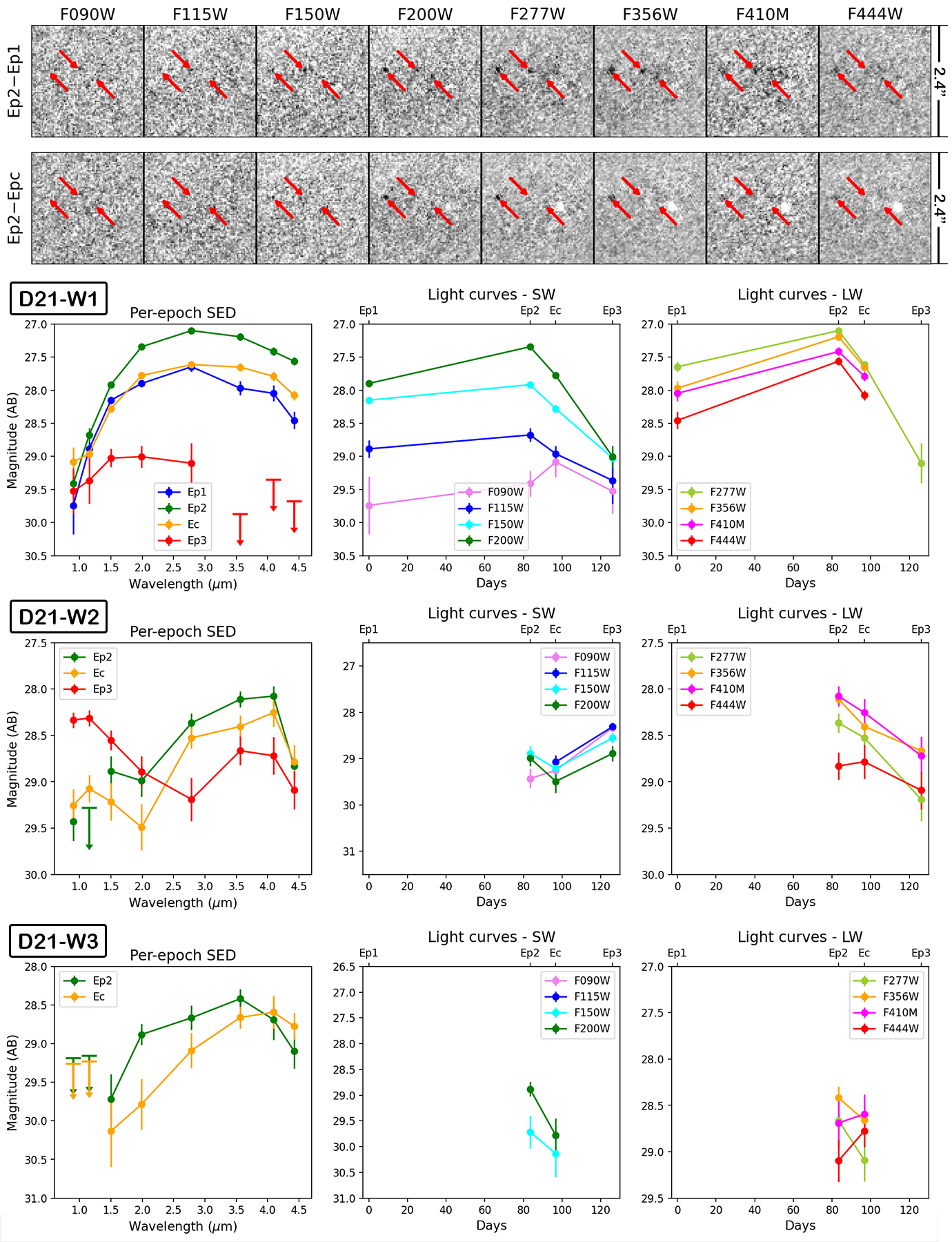
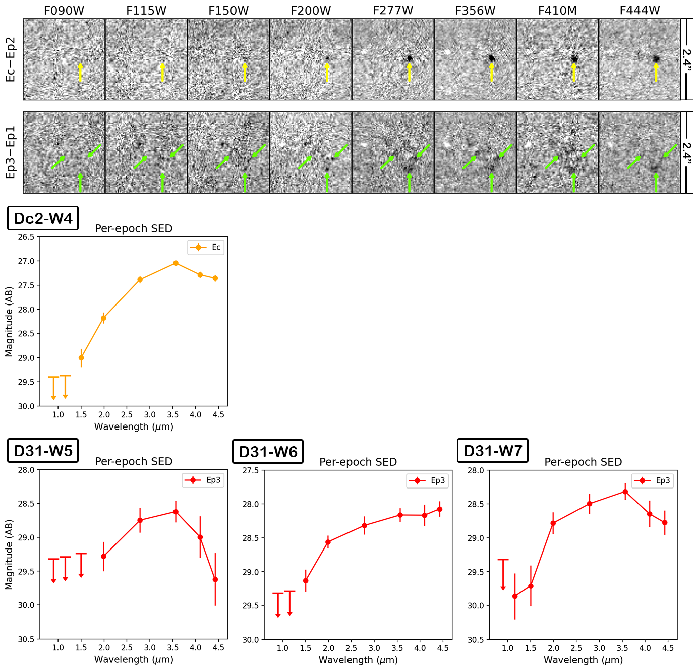
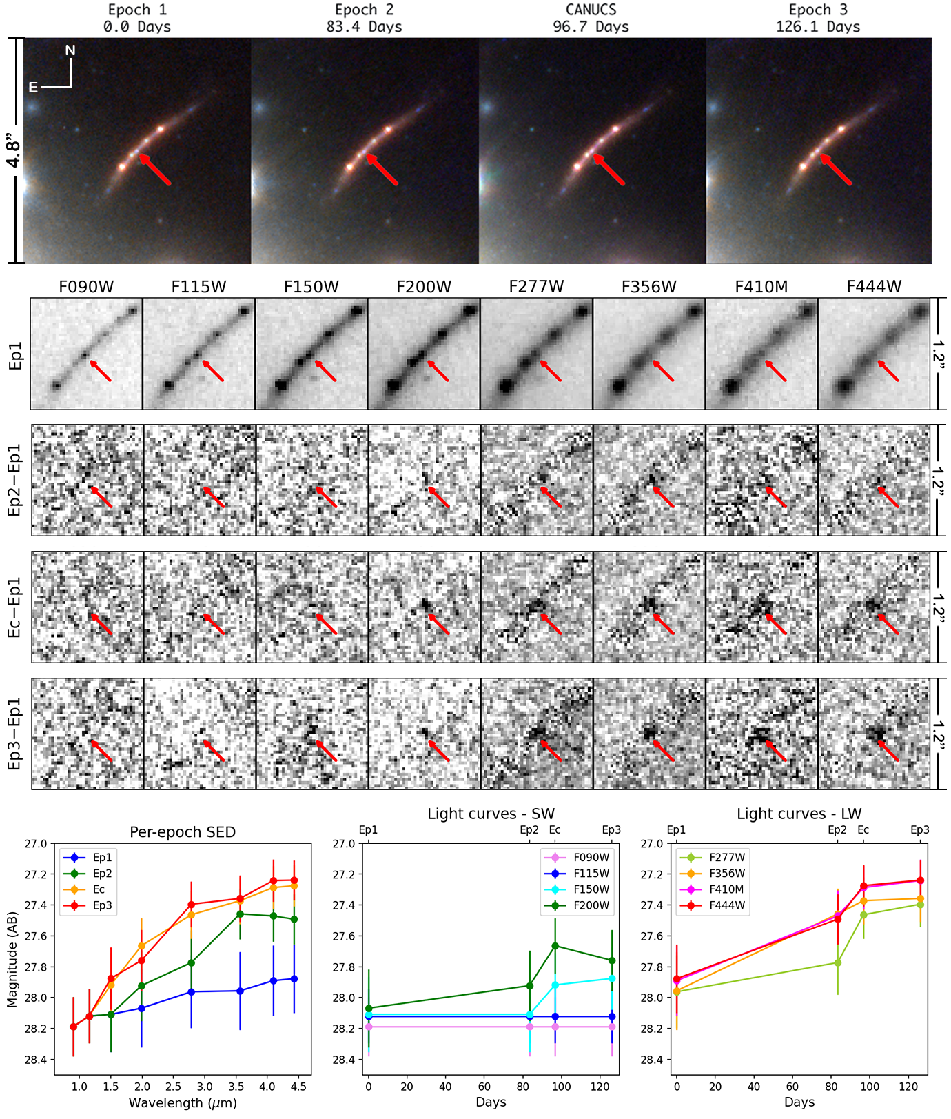
Figure 2 shows the positions of the seven transients discovered in this region. The first three letters in their IDs indicate the difference images on which they were first detected in our process; for example, “Dc2” stands for the difference image constructed by subtracting the Ep2 image from the Ec image, and so on. The letter “W” indicates that these are in the Warhol region. The photometric results are listed in Table 2. Figure 3 shows three of them (D21-W1, D21-W2 and D21-W3) that were seen in multiple epochs, while Figure 4 shows the other four (Dc2-W4, D31-W5, D31-W6, D31-W7) that were visible in only a single epoch.
D21-W1 This transient was visible in Ep1, reached its maximum brightness in Ep2, became fainter in Ec, and further declined in brightness in Ep3 but remained visible. It faded more rapidly in the red bands than in the blue ones. At its peak ( mag), it was the brightest among all transients in this region. As it was visible in all epochs, its photometry was done in each epoch individually.
D21-W2 This transient was invisible in Ep1, appeared in Ep2, and slowly varied in the following two epochs. Interestingly, its behaviors in the SW and the LW bands differed: while it decayed with time in the LW bands, it became much brighter in the SW bands in Ep3, especially in the two bluest bands. The photometry was done on the difference images between these epochs and Ep1 (i.e., the D21, Dc1 and D31 images), as this offers a more reliable determination of the background.
D21-W3 This transient was only away from D21-W2 and was also invisible in Ep1. It appeared in Ep2 in F150W and redder bands. It was much weaker in Ec and barely (if at all) visible in Ep3. The photometry was done on the difference images between all other epochs and Ep1. The decline in brightness from Ep2 to Ec is very obvious in the blue bands. The F444W photometry weakly suggests that it might have slightly brightened from Ep2 to Ec, but this is inconclusive because of the large uncertainties. The extracted signals in Ep3 all have , which we consider as non-detections.
Dc2-W4 This event appeared as a sudden brightening in Ec, particularly in the LW bands. As mentioned earlier, Ec was not used to initiate the transient search; this event was found on the difference images involving Ec when inspecting other transients in the Warhol region. While there seems to be a “source” in other epochs at this location, there is no detectable signal in the difference images between Ep1, Ep2, and Ep3. This means that the event happened only in Ec, and it left no trace in any other epochs, including Ep2, which was only 13.3 days prior. The photometry was done on the difference images between Ec and Ep1 (i.e., the Dc1 images).
D31-W5 This transient was seen only in Ep3, as it was only visible in the difference images involving Ep3. It was very close to D21-W3 but was a different transient. It was invisible in the three bluest bands. The photometry was done on the difference images between Ep3 and Ep1 (the D31 images).
D31-W6 and D31-W7 These two transients were also seen only in Ep3. Like D31-W5, the photometry was done on the difference images between Ep3 and Ep1 (the D31 images).
| R.A. | Decl. | Epoch | F090W | F115W | F150W | F200W | F277W | F356W | F410M | F444W | ||
|---|---|---|---|---|---|---|---|---|---|---|---|---|
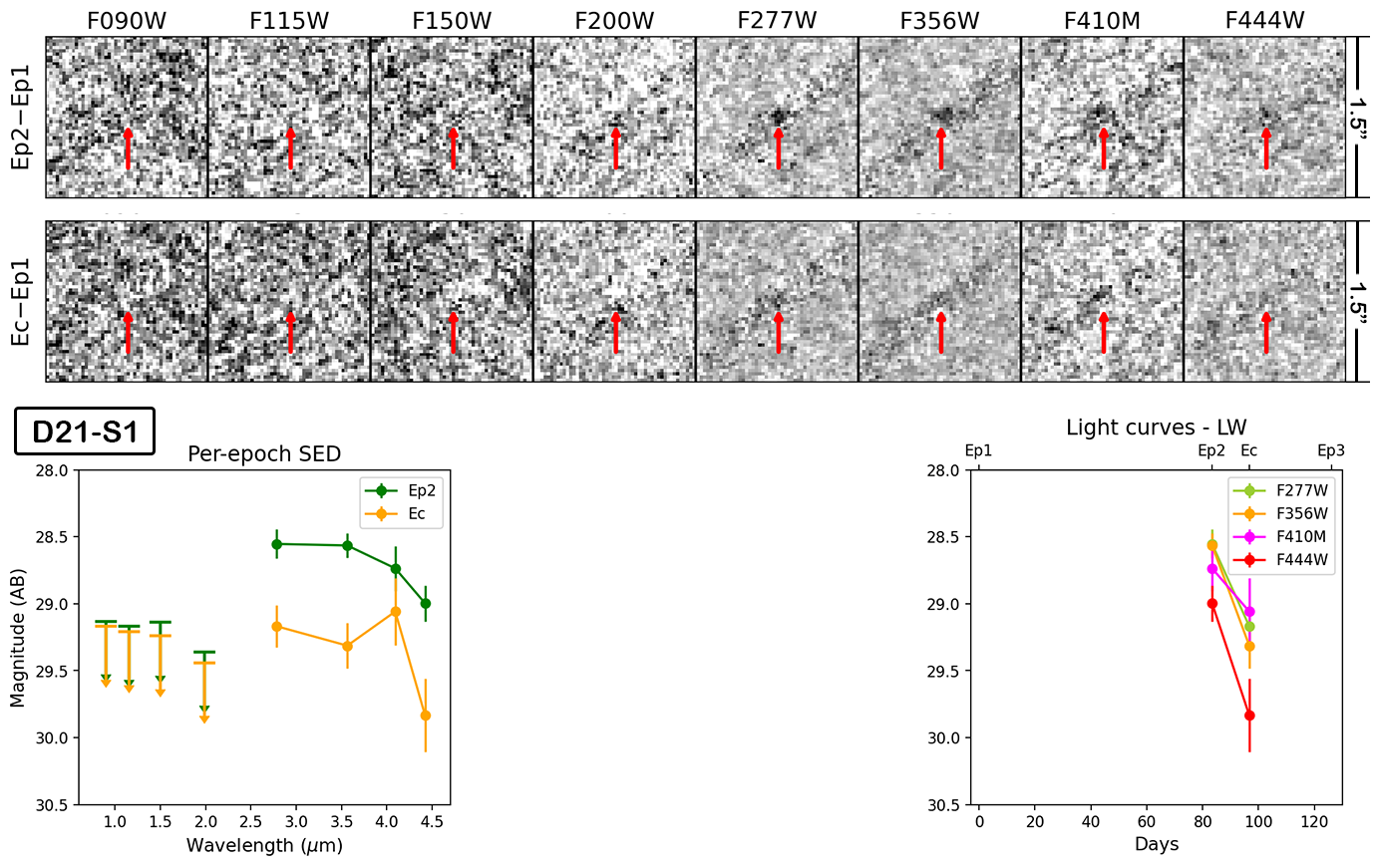
| D21-S1 | 64.03847 | 24.06984 | Ep2 | 29.13 | 29.17 | 29.14 | 29.36 | 28.55±0.11 | 28.56±0.09 | 28.74±0.17 | 29.00±0.14 | 612.6 |
| Ec | 29.17 | 29.21 | 29.24 | 29.44 | 29.17±0.16 | 29.31±0.17 | 29.06±0.25 | 29.83±0.27 | ||||
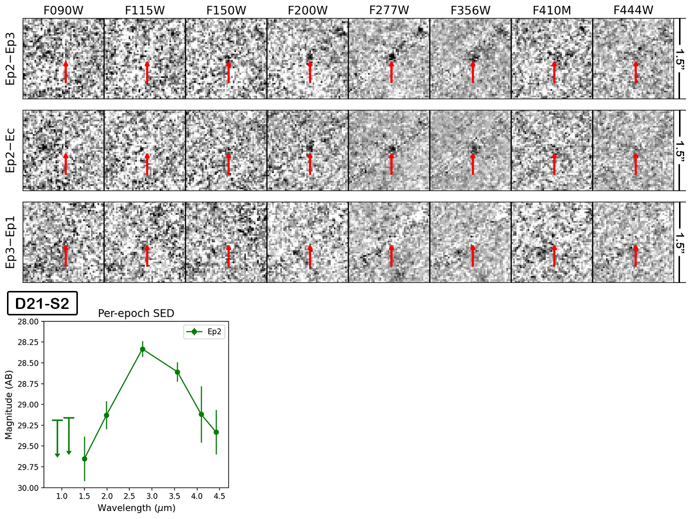
| D21-S2 | 64.03889 | 24.07017 | Ep2 | 29.13 | 29.17 | 29.65±0.27 | 29.13±0.17 | 28.33±0.10 | 28.61±0.12 | 29.12±0.34 | 29.33±0.27 | 87.7 |
| D23-S3 | 64.03874 | 24.07004 | 327.6 | |||||||||
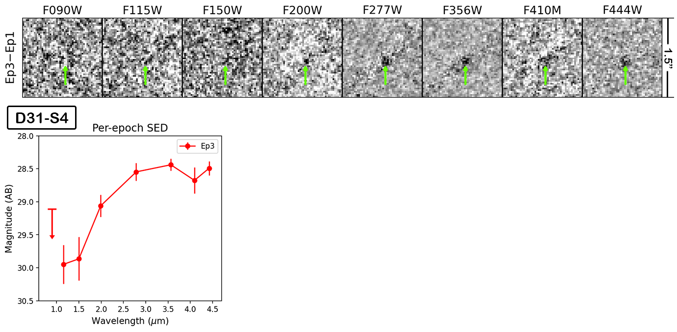
| D31-S4 | 64.03836 | 24.06978 | Ep3 | 29.11 | 29.95±0.29 | 29.86±0.33 | 29.06±0.17 | 28.55±0.13 | 28.44±0.09 | 28.68±0.20 | 28.49±0.11 | 139.0 |
3.2.2 Transients in the Spock region
Figure 5 shows the positions of the four transients in this region. Due to the high brightness of this arc, these transients can only be revealed in the difference images, and none of them is clearly seen in the original images. Their IDs follow the convention of §3.2.1 with “S” to indicate that these transients are in the Spock region. Figures 6 to 9 show the details of these transients. Their photometry (except for D23-S3, see below) is presented in Table 3.
D21-S1 This transient is best detected in the difference images between Ep2 and Ep1 (the D21 images) but is seen only in the LW bands. It became significantly weaker in the difference images between Ec and Ep1 (the Dc1 images) and almost completely disappeared from between Ep3 and Ep1 (the D31 images). All this indicates that it reached the maximum in Ep2 and then faded. Assuming that it was invisible in Ep1, we obtained its magnitudes in Ep2 and Ec by photometry on the difference images between Ep2 and Ep1 (D21) and those between Ec and Ep1 (Dc1).
D21-S2 This transient was detected in the difference images involving Ep2 but not otherwise. Therefore, it is reasonable to assume that this event was caught in Ep2 only. The photometry was done on the difference images between Ep2 and Ep3 (i.e., the D23 images) because this combination offers a cleaner background than others (e.g., the D21 images).
D23-S3 This transient was best detected in the difference images between Ep2 and Ep3 (D23). It appears in the D23 images in F150W through F410M, is barely visible in F444W, and is invisible in F115W and F090W. This transient presents a complicated case that is difficult to understand. First of all, it seems to be an elongated system in the D23 F356W image. In the D23 F200W and F150W images, which have better resolution, this elongated structure is resolved into two components. However, it does not maintain such a two-component structure (or the elongated morphology) consistently in all bands: one of the components (the southern one) is missing from the D23 F277W and F410M images. Second, in the difference images between Ep2 and Ep1 (D21), only the southern component appears, and it appears only in F200W and F150W. Taking the above at the face value, one would infer the following picture: (1) D21-S3 was made of two components; (2) the northern one maintained its brightness from Ep1 to Ep2 and then decayed (not visible in the D21 images but showing up in the D23 images); (3) the southern component brightened in Ep2 but only in F150W and F200W (in the D21 images visible only in F150W and F200W) and then decayed; (4) however, this southern component maintained its brightness from Ep1 through Ep3 in F277W, F356W, and F410M. The last point is inconsistent with the observation that the southern component seems to be present in the D23 F356W image. It is possible to attribute this inconsistency to the weakness of the signals. We attempted PSF fitting on the two components in the D23 images, but the fitting failed in all bands. We have to give up photometry on this transient.

D31-S4 This transient was only detected in the difference images involving Ep3, implying that it appeared in Ep3. It is only 039 away from D21-S1, which already decayed and was invisible in Ep3. The photometry was done on the difference images between Ep3 and Ep1 (D31).
| R.A. | Decl. | Epoch | F090W | F115W | F150W | F200W | F277W | F356W | F410M | F444W | |
|---|---|---|---|---|---|---|---|---|---|---|---|
| 64.03676 | 24.06625 | Ep1 | 28.19±0.19 | 28.12±0.17 | 28.11±0.24 | 28.07±0.25 | 27.96±0.24 | 27.96±0.25 | 27.89±0.23 | 27.88±0.22 | 32.5 |
| Ep2 | 28.19±0.19 | 28.12±0.17 | 28.11±0.24 | 27.92±0.23 | 27.77±0.21 | 27.46±0.16 | 27.47±0.17 | 27.49±0.16 | |||
| Ec | 28.19±0.19 | 28.12±0.17 | 27.92±0.21 | 27.66±0.18 | 27.46±0.16 | 27.37±0.15 | 27.29±0.14 | 27.27±0.13 | |||
| Ep3 | 28.19±0.19 | 28.12±0.17 | 27.88±0.20 | 27.76±0.20 | 27.40±0.15 | 27.36±0.15 | 27.24±0.14 | 27.24±0.13 |
Detecting four transients in this arc in the four epochs is consistent with expectations for this particular arc. Diego et al. (2023a) found that microlensing should produce between one and five transients per pointing in the Spock arc when reaching 29 mag.
3.2.3 A transient in yet another arc
There is one transient identified on an arc at (Bergamini et al., 2021) where no previous transient has been reported. Dubbed “Mothra,” this transient is discussed in detail by Diego et al. (2023b). Figure 10 shows the details of this transient. The knot in which it is located is the faintest among five knots on the arc, but the knot was visible in all four epochs. This transient is best explained by the intrinsic variability of a red supergiant star (in a binary system with a blue supergiant) that is being magnified by a dark milli-lens (Diego et al., 2023b).
The transient behavior is best seen in the difference images between Ep3 and Ep1 (D31) and as well as in those between Ec and Ep1 (Dc1), where it shows up as a strong, red source with decreasing amplitude towards the blue end. It is even visible in the difference images between Ec and Ep2 (Dc2; 13.3 days apart), albeit being much weaker. It is almost invisible in the difference images between Ep3 and Ec (D3c; 29.4 days apart). In other words, this knot was slowly increasing in brightness and reached maximum at around Ec (96.7 days between Ep1 and Ec), and it stayed more or less at its maximum through Ep3 (29.4 days between Ec and Ep3).
Because this transient was caused by the variability of a source that was visible in all epochs, ideally its photometry should be done on the images taken in each epoch. As it is almost blended with a brighter knot 012 to the southeast, one should do PSF fitting on both simultaneously. However, we were only able to obtain reasonable PSF fitting results in Ep1. (The Appendix gives details.) The procedure failed in other epochs, mostly because the light of brightened transient blended with the nearby knot more severely. Therefore, we performed PSF fitting on the difference images between Ep1 and other epochs (Figure 10) and then added the excess fluxes extracted in this way to the Ep1 SED to obtain the SEDs in other epochs. The results are presented in Table 4 and are also shown in the bottom row of Figure 10.
| R.A. | Decl. | Epoch | F090W | F115W | F150W | F200W | F277W | F356W | F410M | F444W | |||
|---|---|---|---|---|---|---|---|---|---|---|---|---|---|
| SN01 | 64.02954 | 24.09022 | Ep1 | 26.84±0.05 | 26.85±0.04 | 27.25±0.03 | 27.73±0.04 | 28.29±0.07 | 29.82* | 29.24* | 29.49* | 2.205 | 2.9 |
| Ep2 | 30.70±0.41 | 29.14±0.10 | 27.68±0.04 | 27.16±0.02 | 27.36±0.04 | 27.47±0.04 | 27.55±0.05 | 27.64±0.06 | |||||
| Ec | 28.73* | 29.76±0.23 | 27.98±0.04 | 27.30±0.03 | 27.56±0.04 | 27.55±0.04 | 27.55±0.06 | 27.72±0.07 | |||||
| Ep3 | 28.87* | 29.80±0.24 | 28.17±0.05 | 27.42±0.03 | 27.63±0.04 | 27.74±0.05 | 27.78±0.07 | 27.96±0.08 | |||||
| SN02 | 64.04421 | 24.07449 | Ep2 | 28.77±0.11 | 27.85±0.06 | 27.44±0.05 | 27.31±0.04 | 27.35±0.06 | 27.60±0.08 | 27.52±0.09 | 27.68±0.08 | 0.793 | 1.9 |
| Ec | 29.20±0.16 | 28.09±0.06 | 27.62±0.04 | 27.39±0.04 | 27.50±0.07 | 27.71±0.07 | 27.85±0.11 | 28.07±0.11 | |||||
| Ep3 | 29.71±0.31 | 28.04±0.09 | 27.76±0.06 | 27.51±0.06 | 27.51±0.08 | 27.54±0.08 | 27.52±0.08 | 27.88±0.10 |
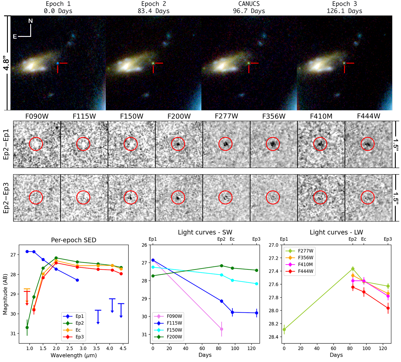
3.2.4 Two likely supernovae
There were two transients associated with galaxies that are only moderately magnified. Both transients were detected in multiple epochs, and neither was seen in the HFF data. Based on their light curves, we believe that they are SNe. Their physical interpretations will be detailed in a forthcoming paper (Wang et al., in prep.). Their photometry is presented in Table 5.
SN01 We initially reported this event (Yan et al., 2023) based on the data from Ep1 and Ep2. Figure 11 shows the color images of the transient and its vicinity in the four epochs. The transient appeared as a blue source in Ep1 and then became very red in the subsequent epochs. The difference images show that its F200W and redder light reached maximum in Ep2. The source is very close to an irregular galaxy, which presumably is the host. The CANUCS NIRISS slitless spectroscopy shows that this galaxy is at (C. Willot, private communication). Because the transient was visible in all epochs, its photometry should be done on the images in individual epochs. To minimize the impact of the contamination from the host galaxy, the photometry was done by PSF fitting. The results are shown in Figure 11.
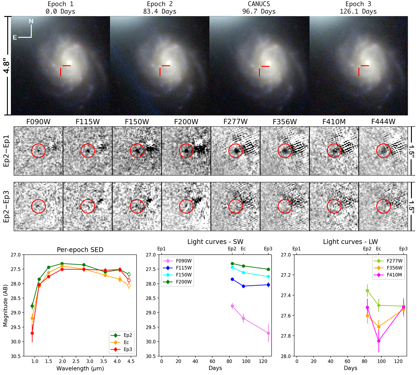
SN02 This transient was found within a spiral galaxy identified at (redshift based on Caminha et al. 2017). The transient was invisible in Ep1 and appeared in Ep2. From the difference images, this transient was brightest in most bands in Ep2 and then slightly decayed in Ec and Ep3. The photometry in Ep2, Ec, and Ep3 was done on the difference images between Ep2 and Ep1 (D21), Ec and Ep1 (Dc1), and Ep3 and Ep1 (D31). In these difference images, the transient’s neighbourhood is affected by the strong residuals from imperfect subtraction of the host-galaxy bulge. PSF-fitting photometry reduced but did not eliminate the contamination.
4 Discussion
The NIRCam data used here were produced by only half of the NIRCam field of view (module B). Because of the different field orientations at different times, the area overlapped in all four epochs amounts to only 3.98 arcmin2. Those data resulted in 14 robust transients, the largest number of transients ever found within such a small area. There are two reasons for this high transient production rate. First, the high sensitivity of NIRCam allows searching for transients to an unprecedented depth. The vast majority of our transients were fainter than 27.0 mag even at their peaks and were fainter than 28.0 mag most of the time in most bands. The PEARLS observations had exposure times of 0.8–1 hours per band per epoch, and the data reach 5 limits of 28.5–30.0 mag (within a 02-radius aperture). This is deep enough to validate the transients in multiple bands. Second, M0416 includes two regions extremely magnified by the cluster, the Warhol and the Spock arcs, which are known to have produced a number of caustic transients in the previous studies with HST. Both arcs are at relatively low redshifts (), which facilitates the detection of luminous stars in them. In our data spanning 126 days, these two regions contributed seven and four transients, respectively, making them the most productive transient “factories” known. In addition, our search found a transient in another arc (the “Mothra” arc) where no transient had been seen previously. As mentioned above (and to be discussed in detail in forthcoming papers), these transients are most likely stars in the lensed arcs that were temporarily magnified by an extra factor by micro-lensing. Studying such transients remains the only direct way to study individual stars at cosmological distances and therefore should be pursued by JWST in the coming years. These transients might occur very frequently. For example, Dc2-W4 in the Warhol region appeared in Ec but was not seen in either Ep2 (13.6 days earlier) or Ep3 (29.4 days later). A monitoring cadence of 10 days (5 days in the rest frame) would potentially reveal more fast transients like Dc2-W4. This possibility is worth exploring with JWST in the near future.
In addition to the 12 transients in the highly magnified arcs, we also discovered two transients in regions that are only moderately magnified (–3). They are most likely SNe, and with intrinsic, post-peak brightnesses of 28.5 mag, they were bright enough to have been discovered even without the lensing magnification. Taken at face value, discovering two SNe in 3.98 arcmin2 implies a SN surface density of 0.5 arcmin-2 integrated to when monitored over 126 days. This frequency is broadly consistent with expectations (Wang et al., 2017; Regős & Vinkó, 2019). Both SNe were caught near their maxima (in the rest-frame visible range) by the Ep2 observations, which were taken 83.4 days after Ep1. Owing to time dilation, neither transient changed significantly in brightness from Ep2 to Ec, which was 96.7 days after Ep1. This suggests that a time cadence of 90 days should be effective in discovering SN-like transients (integrated over all redshifts) and is likely to catch events near their peaks.
Finally, there could be a color bias in the transients reported here. The vast majority of them are very red with the only exception being SN01 in Ep1. Even that source transformed to a red object in Ep2. This may, at least in part, result from the initial selection being based on the F356W difference images. An initial selection based an SW band (e.g., F150W) is possible, although it would be more complex to validate because of the more numerous defects in the SW data.
5 Summary
M0416 has been observed by NIRCam for four epochs, making it the field most intensely monitored by JWST in its Cycle 1. The eight-band data also provide the best near-IR SED sampling to date. This work has identified 14 transients in these four epochs, which spanned 126 days. Twelve transients occurred in three regions highly lensed by the cluster (seven, four, and one in the Warhol, Spock, and Mothra regions, respectively), while the other two happened in two background galaxies that are only moderately magnified (by 2–3). The eight-band photometry enables the construction of the transients’ SEDs from 0.9 to 4.4 m. This is the first time that time-domain studies have such detailed information for interpretation. Further analysis of SEDs and light curves will be presented in forthcoming papers.
This work demonstrates the power of JWST in the study of the transient IR sky. It is now expected that JWST will be able to function for about twenty years, enabling long-term monitoring programs addressing new science never before possible. A new era of IR time-domain science has begun.
The NIRCam data presented in this paper can be accessed via http://dx.doi.org/10.17909/wmmd-ev74 (catalog 10.17909/wmmd-ev74) after the respective proprietary periods.
References
- Amanullah et al. (2010) Amanullah, R., Lidman, C., Rubin, D., et al. 2010, ApJ, 716, 712, doi: 10.1088/0004-637X/716/1/712
- Astropy Collaboration et al. (2013) Astropy Collaboration, Robitaille, T. P., Tollerud, E. J., et al. 2013, A&A, 558, A33, doi: 10.1051/0004-6361/201322068
- Astropy Collaboration et al. (2018) Astropy Collaboration, Price-Whelan, A. M., Sipőcz, B. M., et al. 2018, AJ, 156, 123, doi: 10.3847/1538-3881/aabc4f
- Astropy Collaboration et al. (2022) Astropy Collaboration, Price-Whelan, A. M., Lim, P. L., et al. 2022, ApJ, 935, 167, doi: 10.3847/1538-4357/ac7c74
- Balestra et al. (2016) Balestra, I., Mercurio, A., Sartoris, B., et al. 2016, ApJS, 224, 33, doi: 10.3847/0067-0049/224/2/33
- Bergamini et al. (2021) Bergamini, P., Rosati, P., Vanzella, E., et al. 2021, A&A, 645, A140, doi: 10.1051/0004-6361/202039564
- Bergamini et al. (2023) Bergamini, P., Grillo, C., Rosati, P., et al. 2023, A&A, 674, A79, doi: 10.1051/0004-6361/202244834
- Bertin & Arnouts (1996) Bertin, E., & Arnouts, S. 1996, A&AS, 117, 393, doi: 10.1051/aas:1996164
- Bradley et al. (2023) Bradley, L., Sipőcz, B., Robitaille, T., et al. 2023, astropy/photutils: 1.8.0, 1.8.0, Zenodo, doi: 10.5281/zenodo.7946442
- Bushouse et al. (2023) Bushouse, H., Eisenhamer, J., Dencheva, N., et al. 2023, JWST Calibration Pipeline, 1.9.4, Zenodo, doi: 10.5281/zenodo.7577320
- Caminha et al. (2017) Caminha, G. B., Grillo, C., Rosati, P., et al. 2017, A&A, 600, A90, doi: 10.1051/0004-6361/201629297
- Chen et al. (2019) Chen, W., Kelly, P. L., Diego, J. M., et al. 2019, ApJ, 881, 8, doi: 10.3847/1538-4357/ab297d
- Dawson et al. (2009) Dawson, K. S., Aldering, G., Amanullah, R., et al. 2009, AJ, 138, 1271, doi: 10.1088/0004-6256/138/5/1271
- Diego et al. (2023a) Diego, J. M., Kei Li, S., Meena, A. K., et al. 2023a, arXiv e-prints, arXiv:2304.09222, doi: 10.48550/arXiv.2304.09222
- Diego et al. (2023b) Diego, J. M., Sun, B., Yan, H., et al. 2023b, arXiv e-prints, arXiv:2307.10363, doi: 10.48550/arXiv.2307.10363
- Grillo et al. (2020) Grillo, C., Rosati, P., Suyu, S. H., et al. 2020, ApJ, 898, 87, doi: 10.3847/1538-4357/ab9a4c
- Grillo et al. (2018) —. 2018, ApJ, 860, 94, doi: 10.3847/1538-4357/aac2c9
- Hayden et al. (2021) Hayden, B., Rubin, D., Boone, K., et al. 2021, ApJ, 912, 87, doi: 10.3847/1538-4357/abed4d
- Hoag et al. (2016) Hoag, A., Huang, K. H., Treu, T., et al. 2016, ApJ, 831, 182, doi: 10.3847/0004-637X/831/2/182
- Kaurov et al. (2019) Kaurov, A. A., Dai, L., Venumadhav, T., Miralda-Escudé, J., & Frye, B. 2019, ApJ, 880, 58, doi: 10.3847/1538-4357/ab2888
- Kelly et al. (2015) Kelly, P. L., Rodney, S. A., Treu, T., et al. 2015, Science, 347, 1123, doi: 10.1126/science.aaa3350
- Kelly et al. (2016) —. 2016, ApJ, 819, L8, doi: 10.3847/2041-8205/819/1/L8
- Kelly et al. (2018) Kelly, P. L., Diego, J. M., Rodney, S., et al. 2018, Nature Astronomy, 2, 334, doi: 10.1038/s41550-018-0430-3
- Kelly et al. (2022) Kelly, P. L., Chen, W., Alfred, A., et al. 2022, arXiv e-prints, arXiv:2211.02670, doi: 10.48550/arXiv.2211.02670
- Kelly et al. (2023a) Kelly, P. L., Rodney, S., Treu, T., et al. 2023a, ApJ, 948, 93, doi: 10.3847/1538-4357/ac4ccb
- Kelly et al. (2023b) —. 2023b, Science, 380, abh1322, doi: 10.1126/science.abh1322
- Lotz et al. (2017) Lotz, J. M., Koekemoer, A., Coe, D., et al. 2017, ApJ, 837, 97, doi: 10.3847/1538-4357/837/1/97
- Regős & Vinkó (2019) Regős, E., & Vinkó, J. 2019, ApJ, 874, 158, doi: 10.3847/1538-4357/ab0a73
- Riess et al. (2004) Riess, A. G., Strolger, L.-G., Tonry, J., et al. 2004, ApJ, 607, 665, doi: 10.1086/383612
- Riess et al. (2018) Riess, A. G., Rodney, S. A., Scolnic, D. M., et al. 2018, ApJ, 853, 126, doi: 10.3847/1538-4357/aaa5a9
- Rodney et al. (2018) Rodney, S. A., Balestra, I., Bradac, M., et al. 2018, Nature Astronomy, 2, 324, doi: 10.1038/s41550-018-0405-4
- Suzuki et al. (2012) Suzuki, N., Rubin, D., Lidman, C., et al. 2012, ApJ, 746, 85, doi: 10.1088/0004-637X/746/1/85
- Vanzella et al. (2021) Vanzella, E., Caminha, G. B., Rosati, P., et al. 2021, A&A, 646, A57, doi: 10.1051/0004-6361/202039466
- Vega-Ferrero et al. (2018) Vega-Ferrero, J., Diego, J. M., Miranda, V., & Bernstein, G. M. 2018, ApJ, 853, L31, doi: 10.3847/2041-8213/aaa95f
- Wang et al. (2017) Wang, L., Baade, D., Baron, E., et al. 2017, arXiv e-prints, arXiv:1710.07005. https://arxiv.org/abs/1710.07005
- Willott et al. (2022) Willott, C. J., Doyon, R., Albert, L., et al. 2022, PASP, 134, 025002, doi: 10.1088/1538-3873/ac5158
- Windhorst et al. (2018) Windhorst, R. A., Timmes, F. X., Wyithe, J. S. B., et al. 2018, ApJS, 234, 41, doi: 10.3847/1538-4365/aaa760
- Windhorst et al. (2023) Windhorst, R. A., Cohen, S. H., Jansen, R. A., et al. 2023, AJ, 165, 13, doi: 10.3847/1538-3881/aca163
- Yan et al. (2023) Yan, H., Ma, Z., Grogin, N., et al. 2023, Transient Name Server AstroNote, 6, 1
While we used isophotal aperture photometry by SExtractor to search for transients, we used PSF fitting for the final photometry of the transients identified. This approach assumes that transients are all point-like even at the JWST resolution, which should be valid. The reason we adopted the more complicated PSF fitting (as opposed to aperture photometry) was because of background contamination. Our transients were all embedded in highly non-uniform background, and in a lot of cases that still left structures even in the difference images between epochs. In such situations, PSF fitting handles contamination better than any aperture photometry. We did PSF fitting on the 30mas images (as opposed to the 60mas used in the transient identification). The process is outlined below.
We first generated the PSFs using the simulation tool WebbPSF (version 1.1.1) at the pixel scale of 30mas. For each band, PSFs were simulated at 36 evenly distributed positions on each detector, and each simulated PSF was saved as an individual image. All simulated PSFs were 8787 pixels (261261) in size. Then, effective PSFs, referred to as the WPSFs, were built using EPSFBuilder in Photutils. We also constructed empirical PSFs for comparison. The difficulty with those is that the M0416 field does not have many suitable stars. Nevertheless, we were able to find five isolated, unsaturated, and high stars for this purpose. A region of 8787 pixels centered on each star was cut out from the image, and the five cutouts were sent to EPSFBuilder to build the empirical PSF, referred to as the EPSFs. Both types of PSFs were used, and we found only marginal differences. (See below.)
We used the BasicPSFPhotometry function in Photutils (Bradley et al., 2023) to perform PSF fitting. This function allows simultaneous fitting to multiple, overlapping sources when necessary. The non-linear fitting routine LevMarLSQFitter in Astropy (Astropy Collaboration et al., 2013, 2018, 2022) was applied. The routine utilizes least-squares statistics to decide on the best fit. In PSF fitting, the actual area used to fit the model is usually much smaller than the full PSF size, as only the central region has sufficient . Here we found that the optimal fitting area was 1111 pixels, which is about 2.8 the full-width-at-half-maximum of the F356W PSF.
We provided an initial guess of the source’s centroid and flux when running the fit. The former was estimated by visually locating the peak pixel, while the latter was estimated by measuring the aperture flux within a circle of 11 pixels in diameter centered at the initial guess of the location. Tests showed that BasicPSFPhotometry could converge to the same solution even when the initial guesses were widely different. On the other hand, the routine requires an accurate background estimate because it fixes the background to the input value. In most cases, we estimated the background by using the MedianBackground function in Photutils and adopting the 3-clipped median in the image cutouts centered on the transient (i.e., the same image stamps as shown in the figures in the main text) with the sources masked.
Some special cases required tailored treatments of the fitting. For example, leaving both the source location and its flux as free parameters was not feasible for sources of low . In these cases, we fixed the centroid and fit for the flux. For several sources in highly magnified regions, small but significant positional offsets were found between some SW and LW bands. In such cases, we did not force the fit to be centered at the same position; instead, we determined the centroid in different bands individually. As to the background estimate, median statistics were not applicable for sources in extremely non-uniform local backgrounds. For these cases, we estimated the local background value manually in an iterative manner: we subtracted different constants from the image at a step size of 0.005 MJy/sr, performed a PSF fit, and visually examined the residual image to determine the best local background value by eye. Sources that required some of these special treatments were:
-
•
D21-W2 We determined the source’s centroids in the LW bands using the D21 images and in the SW bands using the D31 images. Their centroids in each band were then fixed for all epochs.
-
•
D21-W3 The source’s centroids were determined from the D21 images and then fixed for Ec.
-
•
Dc2-W4 This source’s local background is non-uniform, and we visually examined and selected the best local background value in Ec.
-
•
D31-W5/W6/W7 These sources’ centroids in the SW bands were determined from the D31 F200W image. In the LW bands, they were determined from the D31 F356W image.
-
•
D21-S2 This source’s centroids in the SW bands were determined from the F200W D21 image. In the LW bands, they were determined from the D21 F277W image.
-
•
D31-S4 This source’s centroids in F115W and F150W were fixed to its F200W centroid.
-
•
Mothra (1) In Ep1, this source’s centroid in F444W was fixed to its F410M centroid. (2) The complexity of simultaneously fitting two overlapping sources on a thin arc made it hard to use any automatic approach to estimate the local background. Therefore, we had to tune the background estimate manually as mentioned above. Furthermore, we used the Ep1 difference images between adjacent bands (the bluer image was always PSF-matched to the redder image when constructing the difference) to judge whether the extracted flux in each band was reasonable under each step of background estimate. For example, if the F150W F115W difference image showed a distinct source at the transient location, it meant that the extracted flux in F150W must be higher than that in F115W. This added constraint, while tedious, allowed us to tweak the background values to obtain the most reasonable flux measurements.
In all cases, our PSF-fitting results have been properly normalized by aperture correction. As mentioned above, we used five stars to construct the EPSFs; these five stars were our basis for the aperture correction. We ran PSF fitting on these five stars to obtain their fitted fluxes and also derived their aperture fluxes within the same 1111 pixel areas. The averaged ratio between the two in each band was the multiplicative aperture correction factor, which we applied to the outputs from BasicPSFPhotometry.
In the end, there are only marginal differences between the results based on the WPSFs and those based on the EPSFs. As the EPSFs were derived using only a small number of stars (total of five), we regard them as being less secure. Therefore, we adopted the WSPF results for our final photometry reported in the tables.