Secant varieties of curves, Ulrich bundles and the arithmetic writhe

Abstract.

We establish a connection between the theory of Ulrich sheaves and ${\mathbb{A}}^{1}$-homotopy theory. For instance, we prove that the ${\mathbb{A}}^{1}$-degree of a morphism between projective varieties, that is relatively oriented by an Ulrich sheaf, is constant on the target even when it is not ${\mathbb{A}}^{1}$-chain connected. Further if an embedded projective variety is the support of a symmetric Ulrich sheaf of rank one, the ${\mathbb{A}}^{1}$-degree of all its linear projections can be read off in an explicit way from the free resolution of the Ulrich sheaf. Finally, we construct an Ulrich sheaf on the secant variety of a curve and use this to define an arithmetic version of Viro’s encomplexed writhe for curves in $\mathbb{P}^{3}$. This can be considered to be an arithmetic analogue of a link invariant.

1. Introduction

In the emerging field of ${\mathbb{A}}^{1}$-enumerative geometry [KW19, Lev20, KW21], building upon the ${\mathbb{A}}^{1}$-homotopy theory developed by Morel and Voevodsky [MV99], solutions to enumerative problems over a field $K$ are counted in the Grothendieck–Witt group $\operatorname{GW}(K)$ of this field in a way that the result does not depend on the chosen instance of the enumerative problem. Typical examples of enumerative problems whose solutions can be “arithmetically enriched” in this way include among others the 27 lines on a cubic surface [KW21], Bézout’s theorem [McK21] or Gromov–Witten invariants [KLSW23]. Results of this type are mostly achieved by studying arithmetic versions of topological invariants like the Euler characteristic [Lev19] or the Brouwer degree [Mor12, KW19]. Here we focus on the latter, namely the ${\mathbb{A}}^{1}$-degree a morphism of smooth schemes as defined in [KLSW23, PW21]. Like in the classical case it can be computed as a sum of local degrees. It is constant over all points in the target $Y$ which can be connected by a chain of affine lines. We explore the connection of this notion of ${\mathbb{A}}^{1}$-degree to the theory of Ulrich sheaves. A coherent sheaf ${\mathcal{F}}$ on a scheme $X$ is called $f$-Ulrich, with respect to a morphism $f\colon X\to Y$ if $f_{*}{\mathcal{F}}\cong{\mathcal{O}}_{Y}^{\oplus t}$ for some natural number $t>0$. If $X\subset\mathbb{P}^{n}$ is a closed subscheme, then one defines a coherent sheaf ${\mathcal{F}}$ on $X$ to be an Ulrich sheaf per se if it is $\pi$-Ulrich for any finite surjective linear projection $\pi\colon X\to\mathbb{P}^{k}$. Ulrich sheaves satisfy a plethora of nice properties and there has been ample interest in the question whether every closed subvariety of $\mathbb{P}^{n}$ carries an Ulrich sheaf [ES03, Bea18]. After recalling preliminaries on Ulrich sheaves in Section 3 and on the ${\mathbb{A}}^{1}$-degree in Section 4.1, we study in Section 4 morphisms that are relatively oriented by an Ulrich sheaf: in the context of ${\mathbb{A}}^{1}$-homotopy theory a relative orientation of a finite surjective morphism $f\colon X\to Y$ of non-singular $K$-varieties is an isomorphism

$$\psi\colon L\otimes L\to\operatorname{{\mathscr{H}om}}(\det{\mathcal{T}}_{X},f^{*}\det{\mathcal{T}}_{Y})$$

where $L$ is a line bundle on $X$ and ${\mathcal{T}}_{X},{\mathcal{T}}_{Y}$ are the tangent bundles on $X$ and $Y$ respectively. We prove that if $L$ is $f$-Ulrich, then the ${\mathbb{A}}^{1}$-degree of $f$ is constant on all of $Y$ — even at points that cannot be connected by affine lines in $Y$ (4.17). If $\pi\colon X\to\mathbb{P}^{k}$ is a finite surjective linear projection from a closed subvariety $X\subset\mathbb{P}^{n}$ which carries a symmetric Ulrich sheaf ${\mathcal{F}}$ of rank one, then we prove in 4.28 that $\pi$ is relatively oriented by ${\mathcal{F}}$ in a natural way and in 4.32 we show that the ${\mathbb{A}}^{1}$-degree of $\pi$ can be computed from the linear resolution of ${\mathcal{F}}$. More precisely, there is a symmetric matrix whose entries are linear forms on $\wedge^{k+1}H^{0}(\mathbb{P}^{n},{\mathcal{O}}_{\mathbb{P}^{n}}(1))$ such that, when plugging in $s_{0}\wedge\cdots\wedge s_{k}$, the class of the resulting matrix in $\operatorname{GW}(K)$ is the ${\mathbb{A}}^{1}$-degree of the linear projection $X\to\mathbb{P}^{k}$ defined by the sections $s_{0},\ldots,s_{k}$.

In Section 5 we construct a symmetric Ulrich sheaf of rank one on the secant variety of any curve $C\subseteq\mathbb{P}^{n}$ with the property that the line bundle $\mathcal{O}_{C}(1)$ is $3$-very ample. In Section 6 we then use this to define an arithmetic version of the writhe. Recall that the writhe of an oriented link diagram is defined to be the sum of the orientations of its crossings — the so-called local writhe numbers (see Figure 1).

Figure 1. Local writhe numbers.

While the writhe is unaffected by Reidemeister moves of type II and III, a Reidemeister move of type I changes the writhe by $\pm 1$. In particular, given an oriented spatial link, the writhe of the link diagram obtained from a projection to the plane may depend on the center of projection. For real algebraic curves Viro [Vir01] showed that this issue can be circumvented by also assigning a local writhe to isolated real nodes of a planar projection of the curve: He defined the encomplexed writhe number as the sum over all local writhe numbers, including those at isolated nodes, and proved that this does not depend on the center of projection. This invariant played a major role in the recent breakthrough on real algebraic links by Mikhalkin and Orevkov [MO19].

In Section 6 we generalize Viro’s construction to oriented space curves $C\subset\mathbb{P}^{3}$ over arbitrary ground fields. The resulting invariant, the arithmetic writhe, is an element of $\operatorname{GW}(K)$. We prove that when the line bundle ${\mathcal{O}}_{C}(1)$ is $3$-very ample, the arithmetic writhe does not depend on the center of projection by realizing it as the ${\mathbb{A}}^{1}$-degree of a suitable morphism. The arithmetic writhe can be thus considered an arithmetic version of a link invariant. It can also be interpreted as an enriched count of secant lines to $C$ which pass through a fixed point $p\in\mathbb{P}^{3}\setminus C$ which does not depend on the choice of $p$.

Figure 2. When applying a Reidemeister move of type I to a real algebraic curve, a crossing of two arcs becomes an isolated node.

2. Notation and conventions

Let $K$ always denote a field. By a $K$-variety we mean an integral, separated scheme of finite type over $K$. We will use the word curve to denote a projective, nonsingular $K$-variety of dimension $1$. If $X$ is a scheme and $x\in X$, then we denote by $\kappa(x)$ the residue field of $X$ at $x$. If $A,B$ are two divisors on a smooth variety $X$ we write $A\sim B$ to denote that $A$ is linearly equivalent to $B$.

3. Ulrich sheaves

We first recall the basic properties of Ulrich sheaves as introduced in [ES03]. Consider the projective space $\mathbb{P}^{n}$ and the corresponding homogeneous coordinate ring $S=K[x_{0},\dots,x_{n}]$. Let $\mathcal{F}$ be a coherent sheaf on $\mathbb{P}^{n}$ with scheme-theoretic support $\iota\colon X\hookrightarrow\mathbb{P}^{n}$ of pure dimension $k>0$ and codimension $c=n-k$. Let also $\Gamma_{*}(\mathcal{F})=\oplus H^{0}(\mathcal{F}(q))$ be the module of twisted global sections, seen as a graded $S$-module. The following important equivalence was proven in [ES03, Theorem 2.1]:

Definition 3.1 (Ulrich sheaf).

The sheaf $\mathcal{F}$ is called an Ulrich sheaf if it satisfies one of the following equivalent conditions:

1. $\Gamma_{*}(\mathcal{F})$ has a linear minimal free resolution as an $S$-module:

   $$\mathbf{F}:\qquad 0\longrightarrow F_{c}\overset{\varphi_{c}}{\longrightarrow}F_{c-1}\overset{\varphi_{c-1}}{\longrightarrow}\dots\overset{\varphi_{2}}{\longrightarrow}F_{1}\overset{\varphi_{1}}{\longrightarrow}F_{0}\longrightarrow\mathcal{F}\longrightarrow 0$$

   where $F_{i}$ is a direct sum of copies of $S(-i)$.

2. $H^{i}(X,{\mathcal{F}}(-i))=0$ for $i>0$ and $H^{i}(X,{\mathcal{F}}(-i-1)=0$ for $i<k$.

3. if $\pi\colon X\to\mathbb{P}^{k}$ is a finite surjective linear projection then $\pi_{*}\iota^{*}{\mathcal{F}}\cong{\mathcal{O}}_{\mathbb{P}^{k}}^{\oplus t}$ for a certain $t>0$.

The resolution of $\mathcal{F}$ can be used to compute a Chow form of $X$. Recall that this is a polynomial in the Plücker coordinates of the Grassmannian ${\mathbb{G}}(c-1,n)$ that cuts out the locus of $(c-1)$-planes that intersect $X$. In the coordinate ring of ${\mathbb{G}}(c-1,n)$ it is unique up to a scalar factor. A power of the Chow form can be written as the determinant of a matrix with entries linear forms in the Plücker coordinates [ES03, §3]. This is constructed from the resolution $\mathbf{F}$ as follows: after choosing a basis of each $F_{i}$ the maps $\varphi_{i}$ are given by matrices $A_{i}$ whose entries are linear forms in the variables $x_{0},\ldots,x_{n}$. We consider these linear forms as degree one elements of the tensor algebra $\textnormal{T}(K^{n+1})^{\vee}$ and define $\gamma(\textbf{F})$ to be the product $A_{1}\cdots A_{c}$ over $\textnormal{T}(K^{n+1})^{\vee}$. The entries of $\gamma(\textbf{F})$ are multilinear forms on $K^{n+1}$ and since $\varphi_{i}\circ\varphi_{i+1}=0$ these multilinear forms are alternating. Therefore, the entries of $\gamma(\textbf{F})$ are elements of $\wedge^{c}(K^{n+1})^{\vee}$ and thus linear in the Plücker coordinates of ${\mathbb{G}}(c-1,n)$. Evaluating $\gamma(\textbf{F})$ at a $(c-1)$-plane $V\subset\mathbb{P}^{n}$ gives a singular matrix if and only if $V$ intersects $X$. This implies that the determinant of $\gamma(\textbf{F})$ is the $\operatorname{rank}({\mathcal{F}})$-th power of the Chow form of $X$. It follows from the definition of the matrix $\gamma(\textbf{F})$ that it actually depends only on the choice of bases of $F_{0}$ and $F_{c}$. Thus $\gamma(\textbf{F})$ is uniquely determined by ${\mathcal{F}}$ up to multiplication from left and right by invertible matrices over $K$. Finally, if there exists a symmetric isomorphism ${\mathcal{F}}\to\operatorname{{\mathscr{E}xt}}^{c}({\mathcal{F}},{\mathcal{O}}_{\mathbb{P}^{n}})(-c)$, then by choosing a suitable basis the determinantal representation can be made symmetric [ES03, §3.1]. We will come back to the symmetric case later.

Example 3.2.

We consider the usual twisted cubic curve $\iota\colon\mathbb{P}^{1}\hookrightarrow\mathbb{P}^{3}$ given by $\iota(s:t)=(s^{3}:s^{2}t:st^{2}:t^{3})$. By 3.1 and a direct computation of cohomology the sheaf ${\mathcal{F}}=\iota_{*}\left({\mathcal{O}}_{\mathbb{P}^{1}}(2)\right)$ is Ulrich. A quick computation using the computer algebra system Macaulay2 [GS] gives us the minimal resolution

where the maps $\varphi_{1}$ and $\varphi_{2}$ are given by the matrices

$$A_{1}=\begin{pmatrix}-x_{1}&-x_{2}&-x_{2}&-x_{3}&-x_{3}&0\\ x_{0}&0&x_{1}&0&x_{2}&-x_{3}\\ 0&x_{0}&0&x_{1}&0&x_{2}\end{pmatrix},\quad A_{2}=\begin{pmatrix}-x_{2}&x_{1}&0&-x_{0}&x_{0}&0\\ -x_{3}&x_{2}&-x_{2}&0&x_{1}&-x_{0}\\ 0&0&x_{3}&-x_{2}&0&x_{1}\end{pmatrix}^{t}.$$

and one calculates that

$$\gamma(\textbf{F})=\begin{pmatrix}-x_{12}&-x_{13}&x_{23}\\ x_{02}&x_{12}+x_{03}&-x_{13}\\ -x_{01}&-x_{02}&x_{12}\end{pmatrix}$$

where the $x_{ij}$ are the usual Plücker coordinates on ${\mathbb{G}}(1,3)$.

4. Ulrich sheaves and the $\mathbb{A}^{1}$-degree

In this section we discuss a connection of Ulrich sheaves and a recently developed notion of degree in the context of ${\mathbb{A}}^{1}$-enumerative geometry.

4.1. Orientations and $\mathbb{A}^{1}$-degree

In this subsection we recall some preliminaries from ${\mathbb{A}}^{1}$-enumerative geometry, mostly following the exposition of [PW21, §8]. Let $K$ always denote a field.

Definition 4.1 (Spin-orientation).

Let $X$ be a non-singular $K$-variety. A spin-orientation of $X$ is an isomorphism $L\otimes L\to\omega_{X}$ where $L$ is a line bundle on $X$ and $\omega_{X}$ the canonical sheaf. We also say that $X$ is oriented by $L\otimes L\to\omega_{X}$. A theta characteristic of $X$ is a line bundle $L$ such that $L\otimes L$ is isomorphic to $\omega_{X}$.

Example 4.2.

If $X=\mathbb{P}^{n}$ with $n=2h-1$ odd, then ${\mathcal{O}}_{\mathbb{P}^{n}}(-h)$ is a theta characteristic of $X$. If $n$ is even, then $\mathbb{P}^{n}$ does not have a theta characteristic.

Definition 4.3.

Let $X$ be a non-singular $K$-variety and $L$ a theta characteristic. Two spin-orientations $\psi_{1},\psi_{2}\colon L\otimes L\to\omega_{X}$ are equivalent if $\psi_{1}\circ\psi_{2}^{-1}$ is multiplication by a square of a global section of ${\mathcal{O}}_{X}$.

Remark 4.4.

Let $K={\mathbb{R}}$ and $X$ be a non-singular ${\mathbb{R}}$-variety of dimension $n$. Let $\psi\colon L\otimes L\to\omega_{X}$ a spin-orientation. Let $f$ some rational section of $L$ and $\omega=\psi(f\otimes f)$. All zeros and poles of the rational differential $n$-form $\omega$ on $X$ are of even order. It can be shown that this implies the existence of a rational function $g$ on $X$ which is nonnegative wherever it is defined on $X({\mathbb{R}})$ and such that $g\cdot\omega$ does not have any zeros or poles on $X({\mathbb{R}})$. Thus $g\cdot\omega$ defines an orientation on $X({\mathbb{R}})$ in the classical topological sense. It is straight-forward to check that this does not depend on the choices we made and that two spin-orientations that are equivalent in the sense of 4.3 induce the same classical orientation on $X({\mathbb{R}})$.

Example 4.5.

Let $X$ be a curve of genus $g$ over ${\mathbb{R}}$. Then every topological orientation of $X({\mathbb{R}})$ is induced by a spin-orientation $L\otimes L\to\omega_{X}$. This follows for instance from [Gey77, Satz 2.4.c]. However, this is not true in general. For instance, let $X$ be a real K3 surface: since the Picard group of $X$ is torsion-free, there is, up to a scalar multiple, only one spin-orientation on $X$. Thus only two topological orientations on $X({\mathbb{R}})$ arise in this way. However, if $X({\mathbb{R}})$ is not connected, then there exist at least four different topological orientations of $X({\mathbb{R}})$.

There is a relative version of spin-orientations for morphisms [PW21, Definition 7]:

Definition 4.6 (Relative orientation).

Let $f\colon X\to Y$ be a finite surjective morphism of non-singular $K$-varieties. A relative orientation of $f$ is an isomorphism

$$\psi\colon L\otimes L\to\operatorname{{\mathscr{H}om}}(\det{\mathcal{T}}_{X},f^{*}\det{\mathcal{T}}_{Y})$$

where $L$ is a line bundle on $X$ and ${\mathcal{T}}_{X},{\mathcal{T}}_{Y}$ are the tangent bundles on $X$ and $Y$ respectively. Two relative orientations $\psi_{1},\psi_{2}$ as above are equivalent if $\psi_{1}\circ\psi_{2}^{-1}$ is multiplication by a square of a global section of ${\mathcal{O}}_{X}$.

Remark 4.7.

If $f\colon X\to Y$ is a finite surjective morphism of non-singular $K$-varieties with spin-orientations $\psi_{1}\colon L_{1}\otimes L_{1}\to\omega_{X}$ and $\psi_{2}\colon L_{2}\otimes L_{2}\to\omega_{Y}$, then a relative orientation of $f$ is given by the induced isomorphism

$$\psi\colon(L_{1}\otimes f^{*}L_{2}^{\vee})^{\otimes 2}\to\omega_{X}\otimes f^{*}\omega_{Y}^{\vee}.$$

Spin-orientations $\psi_{1}^{\prime}$ and $\psi_{2}^{\prime}$ on $X$ and $Y$ that are equivalent to $\psi_{1}$ and $\psi_{2}$ induce a relative orientation $\psi^{\prime}$ for $f$ that is equivalent to $\psi$.

Recall the set of equivalence classes of nondegenerate symmetric bilinear forms on finite dimensional vector spaces over $K$ form a monoid via the orthogonal sum. The Grothendieck–Witt group $\operatorname{GW}(K)$ of $K$ is the Grothendieck group of this monoid. It is generated by all equivalence classes $\langle a\rangle$ of one-dimensional bilinear forms

$$K\times K\to K,\quad(x,y)\mapsto axy$$

for $a\in K^{\times}$. Note that $\langle a\rangle=\langle ab^{2}\rangle$ for all $b\in K^{\times}$.

For a finite morphism $f\colon X\to Y$ of non-singular oriented $K$-varieties of the same dimension one can define a notion of degree that takes its values in $\operatorname{GW}(K)$. Actually it suffices to make the weaker assumption of requiring $f$ to have a relative orientation $\psi\colon L\otimes L\to\operatorname{{\mathscr{H}om}}(\det{\mathcal{T}}_{X},f^{*}\det{\mathcal{T}}_{Y})$. In this case, let $x\in X$ be a closed point where $f$ is not ramified and set $y=f(x)\in Y$. Note that this in particular requires the field extension $\kappa(x)/\kappa(y)$ to be separable. The differential of $f$ defines a morphism $\operatorname{T}f\colon{\mathcal{T}}_{X}\to f^{*}{\mathcal{T}}_{Y}$ and thus $\kappa(x)$-linear maps:

$$\operatorname{T}_{x}f\colon\operatorname{T}_{x}X\to\operatorname{T}_{y}Y\otimes_{\kappa(y)}\kappa(x),\,\operatorname{J}_{x}f=\det\operatorname{T}_{x}f\colon\det\operatorname{T}_{x}X\to\det\operatorname{T}_{y}Y\otimes_{\kappa(y)}\kappa(x)$$

Two bases of $\operatorname{T}_{x}X$ and $\operatorname{T}_{y}Y$ are called compatible with respect to the relative orientation if the determinant of the linear map that sends one base to the other is an element in the fiber of $\operatorname{{\mathscr{H}om}}(\det{\mathcal{T}}_{X},f^{*}\det{\mathcal{T}}_{Y})$ at $x$ which is the image of a square under $\psi$ [PW21, Definition 8]. After choosing such compatible bases, we can identify the determinant $\operatorname{J}_{x}f$ with an element in $\kappa(x)$. Thanks to the requirement of compatibility, it is straight-forward to check that the class $\langle\operatorname{J}_{x}f\rangle\in\operatorname{GW}(\kappa(x))$ does not depend on the bases. We can also define $\langle\operatorname{J}_{x}f\rangle$ without mentioning bases as follows: taking the fiber of the orientation at $x$ we see that $\operatorname{J}_{x}f=g\cdot\psi(t\otimes t)$, for a certain $t\in L_{x}$ and $g\in\kappa(x)$. Then $\langle\operatorname{J}_{x}f\rangle=\langle g\rangle$.

Then the local ${\mathbb{A}}^{1}$-degree $\deg_{x}^{{\mathbb{A}}^{1}}(f)$ of $f$ at $x$ as the class in $\operatorname{GW}(\kappa(y))$ of the symmetric $K$-bilinear form defined by

(1) $$\operatorname{Tr}_{\kappa(x)/\kappa(y)}\langle\operatorname{J}_{x}f\rangle\colon\,\kappa(x)\times\kappa(x)\to\kappa(y),\,(a,b)\mapsto\operatorname{Tr}_{\kappa(x)/\kappa(y)}(\operatorname{J}_{x}ab).$$

Finally, for a closed point $y\in Y$ outside the branch locus of $f$, one defines the ${\mathbb{A}}^{1}$-degree $\deg_{y}^{{\mathbb{A}}^{1}}(f)$ of $f$ at $y$ as

$$\deg_{y}^{{\mathbb{A}}^{1}}(f)=\sum_{x\in f^{-1}(y)}\deg_{x}^{{\mathbb{A}}^{1}}(f)\in\operatorname{GW}(\kappa(y)).$$

Remark 4.8.

One could argue that Equation 1 is rather a formula for the local ${\mathbb{A}}^{1}$-Brouwer degree [Mor06, KW21] than a definition.

Remark 4.9.

The (local) ${\mathbb{A}}^{1}$-degree only depends on the equivalence class of the relative orientation.

Remark 4.10.

In the case $K={\mathbb{R}}$ the signature of the ${\mathbb{A}}^{1}$-degree of $f\colon X\to Y$ is the topological degree of the restriction of $f$ to the real parts of $X$ and $Y$. This is clear from the description of the local degree in Equation 1 together with the observation that every scaled trace bilinear form ${\mathbb{C}}\times{\mathbb{C}}\to{\mathbb{R}}$ has signature zero.

Definition 4.11.

Let $f\colon X\to Y$ be a relatively oriented finite surjective morphism of non-singular $K$-varieties. If there is an element $d\in\operatorname{GW}(K)$ such that for every closed point $y\in Y$ outside the branch locus we have that

$$\deg_{y}^{{\mathbb{A}}^{1}}(f)=d\otimes_{K}\kappa(y)\in\operatorname{GW}(\kappa(y)),$$

then we say that $\deg^{{\mathbb{A}}^{1}}(f)$ is well-defined and we write $\deg^{{\mathbb{A}}^{1}}(f)=d$.

Remark 4.12.

Note that in the situation of 4.11 writing $\deg^{{\mathbb{A}}^{1}}(f)=d$ is a slight abuse of notation since there might be several different $d\in\operatorname{GW}(K)$ satisfying the requirements from 4.11 — for instance in the case that $Y$ has no $K$-rational points.

Example 4.13.

Let $f\colon X\to Y$ as in 4.11.

1. If $Y$ is ${\mathbb{A}}^{1}$-chain connected in the sense of [PW21, Definition 9], then $\deg^{{\mathbb{A}}^{1}}(f)$ is well-defined by [PW21, Theorem 8]. This remains true under the potentially weaker hypothesis that $Y$ is ${\mathbb{A}}^{1}$-connected [KLSW23, §2.5].

2. If $K={\mathbb{R}}$, then it suffices that $Y({\mathbb{R}})$ is connected in the classical topology.

3. In general $\deg^{{\mathbb{A}}^{1}}(f)$ is not necessarily well-defined, see for example [PW21, Example 16].

4.2. Relative Ulrich sheaves and the ${\mathbb{A}}^{1}$-degree

We now derive a further case when $\deg^{{\mathbb{A}}^{1}}(f)$ is well-defined which is a condition on the relative orientation rather than on the target. Motivated by 3.1(iii) one makes the following definition.

Definition 4.14.

Let $f\colon X\to Y$ a morphism of schemes. A coherent sheaf ${\mathcal{F}}$ on $X$ is called $f$-Ulrich if there exists an integer $t>0$ such that $f_{*}{\mathcal{F}}\cong{\mathcal{O}}_{Y}^{\oplus t}$.

We further recall the following construction of a trace map for differential forms.

Construction 4.15.

[Har83, Exercise III.7.2] Let $f\colon X\to Y$ be a finite surjective morphism of nonsingular varieties over $K$. We recall the construction of a natural trace map $t\colon f_{*}\omega_{X}\to\omega_{Y}$. First let $X=\operatorname{Spec}(B)$ and $Y=\operatorname{Spec}(A)$ be affine, $\dim(X)=\dim(Y)=n$ and $E=\operatorname{Quot}(A)$, $F=\operatorname{Quot}(B)$ the fields of fractions. Choose any nonzero $\omega\in\wedge^{n}\Omega_{A/K}$. Then, for any $\omega^{\prime}\in\wedge^{n}\Omega_{B/K}$, there is a $b\in F$ such that $\omega^{\prime}=b\cdot\omega$. The trace map sends $\omega^{\prime}$ to $t(\omega^{\prime})=\operatorname{tr}_{F/E}(b)\cdot\omega$. Note that while $b$ is not necessarily in $B$, we always have that $t(\omega^{\prime})\in\wedge^{n}\Omega_{A/K}$. In the general, not necessarily affine case the map $t$ is obtained by glueing.

Now let $f\colon X\to Y$ be a finite surjective morphism of non-singular $K$-varieties, relatively oriented by the isomorphism

$$\psi\colon L\otimes L\to\operatorname{{\mathscr{H}om}}(\det{\mathcal{T}}_{X},f^{*}\det{\mathcal{T}}_{Y})=\omega_{X}\otimes f^{*}\omega_{Y}^{-1}.$$

By the projection formula the push-forward of $\psi$ induces a map

$$f_{*}L\otimes f_{*}L\to f_{*}\omega_{X}\otimes\omega_{Y}^{-1}.$$

Tensoring the trace morphism from 4.15 by $\omega_{Y}^{-1}$ we obtain a morphism $f_{*}\omega_{X}\otimes\omega_{Y}^{-1}\to{\mathcal{O}}_{Y}$ which we precompose with the map above to obtain a symmetric $\mathcal{O}_{Y}$-bilinear form $\tilde{\psi}\colon f_{*}L\otimes f_{*}L\to{\mathcal{O}}_{Y}$. The following simple lemma can also be seen as a consequence of [KLSW23, Corollary 3.10], but we give here a self-contained proof.

Lemma 4.16.

Let $f\colon X\to Y$ be a finite surjective morphism of non-singular $K$-varieties, relatively oriented by the isomorphism

$$\psi\colon L\otimes L\to\operatorname{{\mathscr{H}om}}(\det{\mathcal{T}}_{X},f^{*}\det{\mathcal{T}}_{Y}).$$

Let $y\in Y$ a closed point outside the branch locus. The class of the fiber of $\tilde{\psi}$ at $y$ in $\operatorname{GW}(\kappa(y))$ is $\deg_{y}^{{\mathbb{A}}^{1}}(f)$.

Proof.

Let $U\subset Y$ an open affine neighbourhood of $y$ and $V=f^{-1}(U)$. Then we have a finite ring extension $A\subset B$ where $A={\mathcal{O}}_{Y}(U)$ and $B={\mathcal{O}}_{X}(V)$. If we choose $U$ sufficiently small, then $\Omega_{A/K}$ is a free $A$-module and $\Omega_{B/K}$ and $M=L(V)$ are free $B$-modules. Since $y$ is not in the branch locus of $f$ we can, after further shrinking $U$ if necessary, moreover assume that $\Omega_{B/K}=\Omega_{A/K}\otimes_{A}B$. Then there are $a_{1},\ldots,a_{n}\in A$ such that $da_{1},\ldots,da_{n}$ is an $A$-basis of $\Omega_{A/K}$ and $da_{1}\otimes 1,\ldots,da_{n}\otimes 1$ is a $B$-basis of $\Omega_{B/K}$. Let $v_{1},\ldots,v_{n}\in\Omega_{A/K}^{\vee}$ and $w_{1},\ldots,w_{n}\in\Omega_{B/K}^{\vee}$ the dual bases so that $\operatorname{T}_{x}f(w_{i})=v_{i}$ for all $x\in V$, and let $t\in M$ a generator of $M$. Then

$$\psi(t\otimes t)=g\cdot\left((da_{1}\otimes 1)\wedge\cdots\wedge(da_{n}\otimes 1)\right)\otimes(v_{1}\wedge\cdots\wedge v_{n})$$

for some $g\in B^{\times}$. Then it follows that $\langle\operatorname{J}_{x_{i}}f\rangle=\langle g(x_{i})\rangle$. For $s_{1},s_{2}\in M$ we can write $s_{i}=h_{i}\cdot t$ for $i=1,2$ and $h_{i}\in B$. By the definition of $\tilde{\psi}$ we then have

(2) $$\tilde{\psi}(s_{1},s_{2})=\operatorname{Tr}_{B/A}(g\cdot h_{1}\cdot h_{2}).$$

Since $B\otimes_{A}\kappa(y)=\kappa(x_{1})\oplus\cdots\oplus\kappa(x_{r})$, Equation 2 evaluated at $y$ equals

$$\sum_{i=1}^{r}\operatorname{Tr}_{\kappa(x_{i})/\kappa(y)}(g(x_{i})\cdot h_{1}(x_{i})\cdot h_{2}(x_{i})).$$

Therefore, the class of the fiber of $\tilde{\psi}$ at $y$ equals

$$\sum_{i=1}^{r}\operatorname{Tr}_{\kappa(x_{i})/\kappa(y)}\langle g(x_{i})\rangle=\sum_{i=1}^{r}\operatorname{Tr}_{\kappa(x_{i})/\kappa(y)}\langle\operatorname{J}_{x_{i}}f\rangle=\sum_{i=1}^{r}\deg_{x_{i}}^{{\mathbb{A}}^{1}}(f)=\deg_{y}^{{\mathbb{A}}^{1}}(f)$$

where we use that $\langle g(x_{i})\rangle=\langle\operatorname{J}_{x_{i}}f\rangle$. ∎

Passing from $\tilde{\psi}\colon f_{*}L\otimes f_{*}L\to{\mathcal{O}}_{Y}$ to global sections, we obtain a symmetric bilinear form

$$\bar{\psi}\colon H^{0}(Y,f_{*}L)\times H^{0}(Y,f_{*}L)\to H^{0}(Y,{\mathcal{O}}_{Y}).$$

In the case that $H^{0}(Y,{\mathcal{O}}_{Y})=K$, this is a symmetric $K$-valued bilinear form.

Theorem 4.17.

Let $f\colon X\to Y$ be a finite surjective morphism of non-singular $K$-varieties, relatively oriented by the isomorphism

$$\psi\colon L\otimes L\to\operatorname{{\mathscr{H}om}}(\det{\mathcal{T}}_{X},f^{*}\det{\mathcal{T}}_{Y}).$$

If $L$ is $f$-Ulrich and $H^{0}(Y,{\mathcal{O}}_{Y})=K$, then the $K$-bilinear form

$$\bar{\psi}\colon H^{0}(Y,f_{*}L)\times H^{0}(Y,f_{*}L)\to K.$$

is nondegenerate. In this case $\deg^{{\mathbb{A}}^{1}}(f)$ is well-defined and equals to the class of $\bar{\psi}$.

Proof.

At every $y\in Y$ the fiber of a $K$-basis of $H^{0}(Y,f_{*}L)$ is a $\kappa(y)$ basis of the fiber of $f_{*}L$ at $y$ because $L$ is $f$-Ulrich. Therefore, the fiber of $\tilde{\psi}$ at $y$ is isometric to $\bar{\psi}\otimes_{K}\kappa(y)$. Now the claim follows from 4.16. ∎

Example 4.18.

Let $X$ be a smooth projective curve and $f\colon X\to\mathbb{P}^{1}$ a finite surjective morphism. Every relative orientation of $f$ is given by a line bundle of the form $L=M(1)$ where $M$ is a theta characteristic on $X$. Then $L$ is $f$-Ulrich if and only if $h^{0}(M)=0$. In particular, for $X=\mathbb{P}^{1}$ every relative orientation is given by an Ulrich line bundle.

One has the following converse of 4.16.

Lemma 4.19.

Let $f\colon X\to Y$ be a finite surjective morphism of non-singular complete $K$-varieties, relatively oriented by the isomorphism

$$\psi\colon L\otimes L\to\operatorname{{\mathscr{H}om}}(\det{\mathcal{T}}_{X},f^{*}\det{\mathcal{T}}_{Y})$$

and assume that $Y$ is geometrically irreducible. The following are equivalent:

1. $L$ is $f$-Ulrich.

2. $\bar{\psi}$ is nondegenerate and for every closed point $y\in Y$ one has

   $$\deg_{y}^{{\mathbb{A}}^{1}}(f)=\bar{\psi}\otimes_{K}\kappa(y)\in\operatorname{GW}(\kappa(y)).$$

Proof.

4.17 proves that $(1)$ implies $(2)$. On the other hand, condition $(2)$ implies that $\bar{\psi}$ is nondegenerate and for $y\in Y$

$$\dim(H^{0}(X,L))=\operatorname{rank}(\bar{\psi})=\operatorname{rank}(\deg_{y}^{{\mathbb{A}}^{1}}(f))=\deg(f).$$

Therefore, by [HK23, Theorem 4.8] the line bundle $L$ is $f$-Ulrich. ∎

We conclude this section with two examples showing that the two sufficient conditions for the ${\mathbb{A}}^{1}$-degree being well-defined, that we have seen here, do not imply each other.

Example 4.20.

Consider a smooth plane cubic curve $X\subset\mathbb{P}^{2}$ and let $f\colon X\to\mathbb{P}^{1}$ the linear projection from a point not on $X$. Then $f$ is relatively oriented by

$$\psi\colon{\mathcal{O}}_{X}(1)\otimes{\mathcal{O}}_{X}(1)\to{\mathcal{O}}_{X}(2)\cong\operatorname{{\mathscr{H}om}}(\det{\mathcal{T}}_{X},f^{*}\det{\mathcal{T}}_{\mathbb{P}^{1}}).$$

However, the line bundle ${\mathcal{O}}_{X}(1)$ is not $f$-Ulrich because it violates part (ii) of 3.1. Since $\dim(H^{0}(X,{\mathcal{O}}_{X}(1))=3=\deg(f)$, this implies in particular that $\bar{\psi}$ cannot be a nondegenerate bilinear form. On the other hand, the target $\mathbb{P}^{1}$ is clearly ${\mathbb{A}}^{1}$-chain connected.

Example 4.21.

Assume here that the characteristic of $K$ is not $2$ or $3$, and consider the smooth sextic curve $X$ in $\mathbb{P}^{3}$ defined over ${\mathbb{Q}}$ by the two equations

$$Q=x_{1}^{2}+x_{2}^{2}-x_{3}^{2}\textnormal{ and }T=x_{0}^{3}+x_{1}^{3}+x_{2}^{3}$$

and the smooth cubic curve $Y$ in $\mathbb{P}^{2}$ defined by $T$. The linear projection from the point $(0:0:0:1)$ defines a finite surjective morphism $f\colon X\to Y$ of degree two. The ramification divisor of $f$ is the zero divisor of $x_{3}$ on $X$. This shows that

$$\operatorname{{\mathscr{H}om}}(\det{\mathcal{T}}_{X},f^{*}\det{\mathcal{T}}_{Y})\cong{\mathcal{O}}_{X}(1).$$

Furthermore, the zero divisor of $x_{2}-x_{3}$ on $X$ is of the form $2D$ where $D$ is an effective divisor of degree three because this hyperplane intersects the singular quadric in $\mathbb{P}^{3}$ defined by $Q$ in a line with multiplicity two. Thus the corresponding line bundle $L$ satisfies $L\otimes L\cong{\mathcal{O}}_{X}(1)$. In particular, we obtain a relative orientation

$$L\otimes L\to\operatorname{{\mathscr{H}om}}(\det{\mathcal{T}}_{X},f^{*}\det{\mathcal{T}}_{Y})$$

of $f$. A calculation with the computer algebra system Macaulay2 [GS] further shows that $f_{*}L={\mathcal{O}}_{Y}^{\oplus 2}$. Thus $\deg^{{\mathbb{A}}^{1}}(f)$ is well-defined by 4.17. On the other hand, by Lüroth’s theorem there is no nonconstant morphism ${\mathbb{A}}^{1}\to Y$ and therefore $Y$ is not ${\mathbb{A}}^{1}$-chain connected (actually not even ${\mathbb{A}}^{1}$-connected [AM11, Corollary 2.4.4]). Let us compute the degree of this map using the method of Theorem 4.17. The quadratic form $\bar{\psi}$ is given by the composition:

$$H^{0}(X,\mathcal{O}_{X}(D))\otimes H^{0}(X,\mathcal{O}_{X}(D)) \longrightarrow H^{0}(X,\mathcal{O}_{X}(2D))$$

$$\overset{\sim}{\longrightarrow} H^{0}(X,\mathcal{O}_{X}(R))$$

$$\longrightarrow H^{0}(Y,\mathcal{O}_{Y})$$

where the first map is the multiplication map, the second map is given by the linear equivalence between $2D$ and the ramification divisor $R=\{x_{3}=0\}$ and the last map is the trace. A basis of $H^{0}(X,\mathcal{O}_{X}(D))$ is given by the rational functions $1,\frac{x_{1}}{x_{2}-x_{3}}$ and multiplying them together we obtain the rational functions $1,\frac{x_{1}}{x_{2}-x_{3}},\left(\frac{x_{1}}{x_{2}-x_{3}}\right)^{2}$. These get mapped to the elements $\frac{x_{2}-x_{3}}{x_{3}},\frac{x_{1}}{x_{3}},\frac{x_{1}^{2}}{(x_{2}-x_{3})x_{3}}$ in $H^{0}(X,\mathcal{O}_{X}(R))$, and finally the traces of these are

$$\operatorname{Tr}\left(\frac{x_{2}-x_{3}}{x_{3}}\right)=\frac{x_{2}-x_{3}}{x_{3}}-\frac{x_{2}+x_{3}}{x_{3}}=\frac{-2x_{3}}{x_{3}}=-2,\quad\operatorname{Tr}\left(\frac{x_{1}}{x_{3}}\right)=\frac{x_{1}}{x_{3}}-\frac{x_{1}}{x_{3}}=0\\ \operatorname{Tr}\left(\frac{x_{1}^{2}}{(x_{2}-x_{3})x_{3}}\right)=\frac{x_{1}^{2}}{(x_{2}-x_{3})x_{3}}-\frac{x_{1}^{2}}{(x_{2}+x_{3})x_{3}}=\frac{2x_{1}^{2}}{x_{2}^{2}-x_{3}^{2}}=-2$$

where the last equality comes from the identity $x_{1}^{2}=x_{3}^{2}-x_{2}^{2}$ on $X$. In conclusion, the quadratic form is given by $(\lambda,\mu)\mapsto-2\lambda^{2}-2\mu^{2}$ so that the $\mathbb{A}^{1}$-degree is $\langle-2\rangle+\langle-2\rangle$.

4.3. Symmetric Ulrich sheaves

Let us first set up some notation. We let $S=\Gamma_{*}({\mathcal{O}}_{\mathbb{P}^{n}})=\oplus_{j\in{\mathbb{Z}}}\Gamma(\mathbb{P}^{n},{\mathcal{O}}_{\mathbb{P}^{n}}(j))$. If $M$ is a graded $S$-module, we denote by $\tilde{M}$ the sheaf associated to $M$ on $\mathbb{P}^{n}$. If $\varphi\colon M\to N$ is a homomorphism of graded $S$-modules, then we denote by $\tilde{\varphi}\colon\tilde{M}\to\tilde{N}$ the associated morphism of quasi-coherent sheaves on $\mathbb{P}^{n}$. One has

$${\mathcal{F}}=\widetilde{\Gamma_{*}({\mathcal{F}})}$$

for any quasi-coherent sheaf ${\mathcal{F}}$ on $\mathbb{P}^{n}$ [Har83, Proposition II.5.15]. Conversely, if $M$ is a finitely generated graded $S$-module of $0pt(M)\geq 2$, one also has $M=\Gamma_{*}(\tilde{M})$ [Eis05, Corollary A.1.13]. This applies in particular when $M$ is Cohen–Macaulay of dimension at least two.

Now let ${\mathcal{F}}$ be an Ulrich sheaf on $\mathbb{P}^{n}$ whose support is a closed subvariety $\iota\colon X\hookrightarrow\mathbb{P}^{n}$ of dimension at least one. Let us denote the rank of $\iota^{*}{\mathcal{F}}$ by $r$ and by $M=\Gamma_{*}({\mathcal{F}})$ the module of twisted global sections over $S$. As explained in Section 3 we can construct from ${\mathcal{F}}$ a matrix $\gamma(\textbf{F})$ obtained from the free resolution F of $M$ whose entries are linear forms in Plücker coordinates and whose determinant is the $r$-th power of the Chow form of $X$. We now recall from [ES03, §3.1] a condition for this matrix to be symmetric. Consider the contravariant functor

(3) $$D\colon{\mathcal{G}}\mapsto\operatorname{{\mathscr{E}xt}}^{c}({\mathcal{G}},{\mathcal{O}}_{\mathbb{P}^{n}}(-c))$$

where $c$ is the codimension of $X$. If ${\mathcal{F}}$ is Ulrich supported on $X$, the sheaf $D({\mathcal{F}})$ is again an Ulrich sheaf with support $X$ and there is a canonical isomorphism $\beta\colon{\mathcal{F}}\to DD{\mathcal{F}}$. A morphism $\sigma\colon{\mathcal{F}}\to D{\mathcal{F}}$ is symmetric if $\sigma=D(\sigma)\circ\beta$. If such a morphism exists, then a suitable choice of bases makes the matrix $\gamma(\textbf{F})$ symmetric [ES03, §3.1].

We will now recall a more explicit description of a minimal free resolution of $M$. To this end recall the following definition.

Definition 4.22.

Let $A=(A_{1},\ldots,A_{s})$ be a tuple of pairwise commuting $m\times m$ matrices over a ring $R$. We can define on $R^{m}$ the structure of an $R[t_{1},\ldots,t_{s}]$-module $P$ by letting $t_{i}$ act on $R^{m}$ via multiplication with the matrix $A_{i}$ from the left. Consider the complex $P\otimes\operatorname{\bf K}(t)$ where $\operatorname{\bf K}(t)$ is the Koszul complex of the sequence $t=(t_{1},\ldots,t_{s})$. We can view this complex as a complex of $R$-modules instead of $R[t_{1},\ldots,t_{s}]$-modules. The resulting complex of free $R$-modules is called the Koszul complex associated to the matrices $A_{1},\ldots,A_{s}$ and we denote it by $\operatorname{\bf K}(A)$. The maps of $\operatorname{\bf K}(A)$ are obtained from the maps of the Koszul complex $\operatorname{\bf K}(t)$ by replacing every occurrance of $t_{i}$ by $A_{i}$ for $i=1,\ldots,s$.

Let $k=n-c$ be the dimension of $X$ and $s_{0},\ldots,s_{k}\in H^{0}(\mathbb{P}^{n},{\mathcal{O}}_{\mathbb{P}^{n}}(1))$ sections that do not have a common zero on $X$. Then the morphism

$$\pi\colon X\to\mathbb{P}^{k},\,x\mapsto(s_{0}(x):\cdots:s_{k}(x))$$

defines a finite surjective morphism. Let $s_{0},\ldots,s_{n}$ a basis of $H^{0}(\mathbb{P}^{n},{\mathcal{O}}_{\mathbb{P}^{n}}(1))$ and consider the inclusion

$$R:=K[s_{0},\ldots,s_{k}]\subset K[s_{0},\ldots,s_{n}]=S$$

of graded polynomial rings. Because ${\mathcal{F}}$ is an Ulrich sheaf, it holds that $\pi_{*}\mathcal{F}\cong\mathcal{O}_{\mathbb{P}^{k}}^{\oplus t}$, so that there is an isomorphism

$$\psi\colon M\to R^{m}$$

of $R$-modules where $m=t\cdot\deg(X)$. Under this identification multiplication by $s_{i}$ can be represented by an $m\times m$ matrix $B_{i}$ with entries from $R_{1}$ for $i=0,\ldots,n$. Let $A_{i}=s_{i}\cdot I_{m}-B_{i}$ where $I_{m}$ is the $m\times m$ identity matrix.

Theorem 4.23.

The Koszul complex $\operatorname{\bf K}(A)$ associated to the matrices $A_{k+1},\ldots,A_{n}$ is a minimal free resolution of $M$. In particular, we can describe $M$ as the cokernel of the matrix $(A_{k+1}\cdots A_{n})$ and $\operatorname{Ext}_{S}^{c}(M,S)(-c)$ as the cokernel of $(A^{t}_{k+1}\cdots A^{t}_{n})$.

Proof.

See [Kum16, Proof of Theorem 6.2.5] or [KS20, Remark 4.8]. ∎

Remark 4.24.

Note that, since the Koszul complex is self-dual, 4.23 also implies that a minimal free resolution of $\operatorname{Ext}_{S}^{c}(M,S)(-c)$ is given by the Koszul complex $\operatorname{\bf K}(A^{t})$ associated to the matrices $A^{t}_{k+1},\ldots,A^{t}_{n}$. This is one way to see that $\operatorname{Ext}_{S}^{c}(M,S)(-c)$ is an Ulrich module.

Corollary 4.25.

There is a natural isomorphism

$$\operatorname{Ext}_{S}^{c}(M,S)(-c)\cong\operatorname{Hom}_{R}(M,R)$$

of $S$-modules. Here the $S$-module structure on $\operatorname{Hom}_{R}(M,R)$ is defined by $(s\varphi)(x):=\varphi(sx)$ for $s\in S$ and $x\in M$.

Proof.

Under the identification

$$\psi^{\vee}\colon R^{m}=\operatorname{Hom}_{R}(R^{m},R)\to\operatorname{Hom}_{R}(M,R)$$

multiplication by $s_{i}$ on $\operatorname{Hom}_{R}(M,S)$ is represented by the $m\times m$ matrix $B^{t}_{i}$. Hence the $S$-module $\operatorname{Hom}_{R}(M,R)$ is isomorphic to the cokernel of $(A^{t}_{k+1}\cdots A^{t}_{n})$ which is $\operatorname{Ext}_{S}^{c}(M,S)(-c)$ by 4.23. It is straight-forward to check that the resulting isomorphism $\operatorname{Ext}_{S}^{c}(M,S)(-c)\to\operatorname{Hom}_{R}(M,R)$ does not depend on the choice of the $R$-module isomorphism $\psi\colon M\to R^{m}$. ∎

The next lemma shows that we can work with $\operatorname{Ext}_{S}^{c}(M,S)$ and $\operatorname{{\mathscr{E}xt}}^{c}({\mathcal{F}},{\mathcal{O}}_{\mathbb{P}^{n}})$ interchangeably.

Lemma 4.26.

Let $N=\operatorname{Ext}_{S}^{c}(M,S)$ and ${\mathcal{G}}=D({\mathcal{F}})$.

1. There is a natural isomorphism of coherent sheaves $\widetilde{N}\cong{\mathcal{G}}$.

2. There is a natural isomorphism of graded $S$-modules $N\cong\Gamma_{*}({\mathcal{G}})$.

Proof.

A minimal free resolution of $M$ gives rise to a free resolution of ${\mathcal{F}}$ of length $c$. Thus by [Har83, Proposition III.6.5] we can compute $\operatorname{{\mathscr{E}xt}}^{c}({\mathcal{F}},{\mathcal{O}}_{\mathbb{P}^{n}}(-c))$ as the cokernel of the dual of the last map of this resolution. This map is induced by the dual of the last map of the resolution of $M$ whose cokernel is $\operatorname{Ext}_{S}^{c}(M,S)$. This implies part (1). Since $N$ is a twist of an Ulrich module and therefore Cohen–Macaulay, we have $N=\Gamma_{*}(\widetilde{N})$ which implies part (2). ∎

Recall that for a finite surjective morphism $f\colon X\to Y$ of noetherian schemes the right adjoint functor of $f_{*}$ (considered as a functor from quasi-coherent sheaves on $X$ to quasi-coherent sheaves on $Y$) can be described as follows. For a quasi-coherent ${\mathcal{O}}_{Y}$-module ${\mathcal{G}}$ the sheaf $\operatorname{{\mathscr{H}om}}_{Y}(f_{*}{\mathcal{O}}_{X},{\mathcal{G}})$ is a quasi-coherent $f_{*}{\mathcal{O}}_{X}$-module. The corresponding quasi-coherent ${\mathcal{O}}_{X}$-module is then $f^{!}{\mathcal{G}}$, see for example [Har83, Exercise III.6.10].

Lemma 4.27.

Let $f\colon X\to Y$ a finite surjective morphism of smooth varieties over $K$. Then $f^{!}{\mathcal{O}}_{Y}$ is a line bundle, naturally isomorphic to $\operatorname{{\mathscr{H}om}}(\det{\mathcal{T}}_{X},f^{*}\det{\mathcal{T}}_{Y})$.

Proof.

This is for example shown in [Kum16, Remark 2.2.19]. ∎

Theorem 4.28.

Let ${\mathcal{F}}$ be an Ulrich sheaf on $\mathbb{P}^{n}$ and $\sigma\colon{\mathcal{F}}\to D{\mathcal{F}}$ an isomorphism. Assume that the support of ${\mathcal{F}}$ is a closed subvariety $\iota\colon X\hookrightarrow\mathbb{P}^{n}$ of dimension $k=\dim(X)>0$ and that $\iota^{*}{\mathcal{F}}$ has rank one. Let $\pi\colon X\to\mathbb{P}^{k}$ a finite surjective linear projection and $U\subset\mathbb{P}^{k}$ an open subset such that $V=\pi^{-1}(U)\subset X$ is smooth. Then there is a natural relative orientation

$$\sigma(\pi|_{V})\colon L\otimes L\to\operatorname{{\mathscr{H}om}}(\det{\mathcal{T}}_{V},(\pi|_{V})^{*}\det{\mathcal{T}}_{U})$$

of $\pi|_{V}$ where $L=(\iota^{*}{\mathcal{F}})|_{V}$.

Proof.

4.25 and 4.26 imply that there is a natural ismorphism

$$\iota^{*}(D{\mathcal{F}})\to\operatorname{{\mathscr{H}om}}_{X}(\iota^{*}{\mathcal{F}},\pi^{!}{\mathcal{O}}_{\mathbb{P}^{k}}).$$

Precomposing this with the pullback of $\sigma$ under $\iota$ gives an isomorphism

$$\iota^{*}({\mathcal{F}})\to\operatorname{{\mathscr{H}om}}_{X}(\iota^{*}{\mathcal{F}},\pi^{!}{\mathcal{O}}_{\mathbb{P}^{k}}).$$

Because every Ulrich sheaf is Cohen–Macaulay, the restriction $(\iota^{*}{\mathcal{F}})|_{V}$ is a line bundle on $V$. Thus restricting to $V$ and tensoring with $\iota^{*}{\mathcal{F}}$ gives the isomorphism

(4) $$(\iota^{*}{\mathcal{F}})|_{V}\otimes(\iota^{*}{\mathcal{F}})|_{V}\to(\pi^{!}{\mathcal{O}}_{\mathbb{P}^{k}})|_{V}=(\pi|_{V})^{!}{\mathcal{O}}_{U}.$$

Finally, by 4.27 we obtain on $V$ the isomorphism

$$(\iota^{*}{\mathcal{F}})|_{V}\otimes(\iota^{*}{\mathcal{F}})|_{V}\to\operatorname{{\mathscr{H}om}}(\det{\mathcal{T}}_{V},(\pi|_{V})^{*}\det{\mathcal{T}}_{U}).\qed$$

Remark 4.29.

One can prove in a similar way that if ${\mathcal{F}}$ is a rank one sheaf on $X$ with an isomorphism $\sigma\colon{\mathcal{F}}\overset{\sim}{\to}D{\mathcal{F}}$, and such that the restriction ${\mathcal{F}}_{|V}$ is a line bundle $L$, then $L$ is a relative orientation for the map $\pi_{|V}\colon V\to U$. This works also when ${\mathcal{F}}$ is not Ulrich. However, when ${\mathcal{F}}$ is Ulrich, the proof of 4.28 shows how to compute the $\mathbb{A}^{1}$-degree of the map $\pi_{|V}$ via Theorem 4.17. We will make this clear in Theorem 4.32

Definition 4.30.

In the situation of 4.28 we call $\sigma(\pi|_{V})$ the relative orientation induced by $\sigma$.

Lemma 4.31.

If the rank of $\iota^{*}{\mathcal{F}}$ is one, then every isomorphism $\sigma\colon{\mathcal{F}}\to D{\mathcal{F}}$ is symmetric.

Proof.

Since ${\mathcal{F}}$ is supported on $X$, it suffices to prove the pullback of the equality $\sigma=D(\sigma)\circ\beta$ under $\iota$. Let $V$ as in 4.28. Since $V$ is dense in $X$, it further suffices to prove the equality on $V$. As in Equation 4 in the proof of 4.28 the isomorphism $\sigma$ induces an isomorphism

$$\rho\colon(\iota^{*}{\mathcal{F}})|_{V}\otimes(\iota^{*}{\mathcal{F}})|_{V}\to(\pi|_{V})^{!}{\mathcal{O}}_{U}$$

and the condition on $\sigma$ being symmetric translates to the condition that $\rho_{x}(a\otimes b)=\rho_{x}(b\otimes a)$ for all $x\in V$ and $a,b\in(\iota^{*}{\mathcal{F}})|_{x}$. Since $(\iota^{*}{\mathcal{F}})|_{V}$ is locally free of rank one, there is $t\in(\iota^{*}{\mathcal{F}})|_{x}$ and $f,g\in{\mathcal{O}}_{X,x}$ such that $a=f\cdot t$ and $b=g\cdot t$. Then

$$\rho_{x}(a\otimes b)=fg\cdot\rho_{x}(t\otimes t)=\rho_{x}(b\otimes a).\qed$$

Now we are ready to state the main result of this section.

Theorem 4.32.

Let ${\mathcal{F}}$ be an Ulrich sheaf on $\mathbb{P}^{n}$ whose support is a closed subvariety $\iota\colon X\hookrightarrow\mathbb{P}^{n}$ of dimension $k>0$ and degree $d$. Assume that the rank of $\iota^{*}{\mathcal{F}}$ is one and let $\sigma\colon{\mathcal{F}}\to D{\mathcal{F}}$ an isomorphism. There is a symmetric $d\times d$ matrix $\Lambda$ whose entries are linear forms on $\wedge^{k+1}H^{0}(\mathbb{P}^{n},{\mathcal{O}}_{\mathbb{P}^{n}}(1))$ such that for all $s_{0}\ldots,s_{k}\in H^{0}(\mathbb{P}^{n},{\mathcal{O}}_{\mathbb{P}^{n}}(1))$ it holds that:

1. $\Lambda(s_{0}\wedge\cdots\wedge s_{k})$ is singular if and only if the $s_{j}$ have a common zero on $X$.

2. If the $s_{j}$ do not have a common zero on $X$ let $\pi\colon X\to\mathbb{P}^{k}$ be the morphism defined by $s_{0},\ldots,s_{k}$ and $U\subset\mathbb{P}^{k}$ an open subset such that $V=\pi^{-1}(U)\subset X$ is smooth. The class of $\Lambda(s_{0}\wedge\cdots\wedge s_{k})$ in $\operatorname{GW}(K)$ equals to $\deg^{{\mathbb{A}}^{1}}(\pi|_{V})$ where $\pi|_{V}$ is relatively oriented by $\sigma(\pi|_{V})$.

Proof.

We first note that by 4.31 the isomorphism $\sigma\colon{\mathcal{F}}\to D{\mathcal{F}}$ is symmetric. Let $M=\Gamma_{*}({\mathcal{F}})$ and let

$$\mathbf{F}:\qquad 0\longrightarrow F_{c}\overset{\varphi_{c}}{\longrightarrow}F_{c-1}\overset{\varphi_{c-1}}{\longrightarrow}\dots\overset{\varphi_{2}}{\longrightarrow}F_{1}\overset{\varphi_{1}}{\longrightarrow}F_{0}\longrightarrow M\longrightarrow 0.$$

a minimal free resolution of $M$. We choose any $S$-basis ${\mathcal{B}}_{0}$ of $F_{0}$. The image of ${\mathcal{B}}_{0}$ under the map $F_{0}\to M$ is sent by $\sigma$ to a generating set of $\operatorname{Ext}^{c}(M,S)(-c)$. A preimage of this generating set in the degree zero part of $\operatorname{Hom}_{S}(F_{c},S)(-c)$ under the natural map $\operatorname{Hom}_{S}(F_{c},S)(-c)\to\operatorname{Ext}^{c}(M,S)(-c)$ is a basis of $\operatorname{Hom}_{S}(F_{c},S)(-c)$ and thus of $\operatorname{Hom}_{S}(F_{c},S)$. We denote by ${\mathcal{B}}_{c}$ the dual of this basis which is a basis of $F_{c}$. We claim that with this choice of bases of $F_{0}$ and $F_{c}$ (and any choice of basis of $F_{i}$ for $0<i<c$) the matrix $\gamma(\mathbf{F})$ has the desired properties. We already know that $\gamma(\mathbf{F})$ is a $d\times d$ matrix whose entries are linear forms on $\wedge^{k+1}H^{0}(\mathbb{P}^{n},{\mathcal{O}}_{\mathbb{P}^{n}}(1))$ which satisfies (1). It thus remains to show that $\gamma(\mathbf{F})$ is symmetric and satisfies (2). To this end let $s_{0}\ldots,s_{k}\in H^{0}(\mathbb{P}^{n},{\mathcal{O}}_{\mathbb{P}^{n}}(1))$ sections that do not have a common zero on $X$. Then, as in the discussion before 4.23, the morphism $\pi\colon X\to\mathbb{P}^{k}$ defined by $s_{0},\ldots,s_{k}$ corresponds to an inclusion of graded polynomial rings

$$R:=K[s_{0},\ldots,s_{k}]\subset K[s_{0},\ldots,s_{n}]=S.$$

We consider the isomorphism

$$\psi\colon M\to R^{d}$$

of $R$-modules which sends the image of ${\mathcal{B}}_{0}$ under the map $F_{0}\to M$ to the standard basis of $R^{d}$. We denote by $B_{i}$ the representing matrix of multiplication by $s_{i}$ with respect to this basis and let $A_{i}=s_{i}\cdot I_{d}-B_{i}$ where $I_{d}$ is the $d\times d$ identity matrix. Further let $\operatorname{\bf K}(A)$ the Koszul complex associated to the matrices $A_{k+1},\ldots,A_{n}$. We then have

(5) $$\gamma(\mathbf{F})\cdot Q=\gamma(\operatorname{\bf K}(A))$$

where $Q$ is the representing matrix of the $R$-bilinear form on $M$ obtained by composing $\sigma\colon M\to\operatorname{Ext}^{c}(M,S)(-c)$ with the natural isomorphism from 4.25 with respect to our chosen basis. Note that $Q$ is a symmetric matrix because $\sigma$ is symmetric which further satisfies

(6) $$QA_{i}=A_{i}^{t}Q$$

for all $i=k+1,\ldots,n$ because $\sigma$ is a homomorphism of $S$-modules. By 4.17 and our choice of relative orientation the class of $Q$ in $\operatorname{GW}(K)$ equals to $\deg^{{\mathbb{A}}^{1}}(\pi|_{V})$. Since $Q$ and $Q^{-1}$ represent the same class in $\operatorname{GW}(K)$ and by Equation 5, it now suffices to show that $\gamma(\operatorname{\bf K}(A))\cdot Q^{-1}$ is symmetric and that $\gamma(\operatorname{\bf K}(A))(s_{0}\wedge\cdots\wedge s_{k})=I_{d}$. To this end we regard $\gamma(\operatorname{\bf K}(A))$ as an alternating multilinear map

$$\left(H^{0}(\mathbb{P}^{n},{\mathcal{O}}_{\mathbb{P}^{n}}(1))^{\vee}\right)^{c}\to\operatorname{Mat}_{d}(K)$$

and use the explicit description

(7) $$\gamma(\operatorname{\bf K}(A))(v_{1},\ldots,v_{c})=\sum_{\tau\in\mathcal{S}_{c}}\textnormal{sgn}(\tau)\cdot A_{k+\tau(1)}(v_{1})\cdots A_{k+\tau(c)}(v_{c})$$

where $v_{1},\ldots,v_{c}\in H^{0}(\mathbb{P}^{n},{\mathcal{O}}_{\mathbb{P}^{n}}(1))^{\vee}$, see [Kum16, Example 6.1.4]. Equation 7 together with Equation 6 now imply

$$\gamma(\operatorname{\bf K}(A))(v_{1},\ldots,v_{c})\cdot Q^{-1} = \sum_{\tau\in\mathcal{S}_{c}}\textnormal{sgn}(\tau)\cdot A_{k+\tau(1)}(v_{1})\cdots A_{k+\tau(c)}(v_{c})\cdot Q^{-1}$$

$$= \sum_{\tau\in\mathcal{S}_{c}}\textnormal{sgn}(\tau)Q^{-1}\cdot A^{t}_{k+\tau(1)}(v_{1})\cdots A^{t}_{k+\tau(c)}(v_{c})$$

$$= Q^{-1}\gamma(\operatorname{\bf K}(A))^{t}(v_{1},\ldots,v_{c}).$$

This shows that $\gamma(\operatorname{\bf K}(A))\cdot Q^{-1}$ is symmetric. Letting $s_{0}^{\vee},\ldots,s_{n}^{\vee}$ be the dual basis of $s_{0},\ldots,s_{n}$ we further have

$$\gamma(\operatorname{\bf K}(A))(s_{0}\wedge\cdots\wedge s_{k}) = \gamma(\operatorname{\bf K}(A))(s_{k+1}^{\vee},\ldots,s_{n}^{\vee})$$

$$= \sum_{\tau\in\mathcal{S}_{c}}\textnormal{sgn}(\tau)\cdot A_{k+\tau(1)}(s_{k+1}^{\vee})\cdots A_{k+\tau(c)}(s_{k+c}^{\vee})$$

$$= I_{d}$$

since $A_{k+i}(s_{k+j}^{\vee})=\delta_{ij}\cdot I_{d}$. This concludes the proof. ∎

Example 4.33.

Consider the rational normal curve $\iota\colon\mathbb{P}^{1}\hookrightarrow\mathbb{P}^{n}$ of degree $n$ and the symmetric Ulrich sheaf ${\mathcal{F}}=\iota_{*}\left({\mathcal{O}}_{\mathbb{P}^{1}}(n-1)\right)$. 4.32 gives an $n\times n$ matrix $\Lambda$ whose entries are linear forms on $\wedge^{2}K[x_{0},x_{1}]_{n}$ such that for all binary forms $p,q\in K[x_{0},x_{1}]_{n}$ we have:

1. $\Lambda(p\wedge q)$ has full rank if and only if $p$ and $q$ are coprime.

2. If $p$ and $q$ are coprime, then the ${\mathbb{A}}^{1}$-degree of the map

   $$\psi\colon\mathbb{P}^{1}\to\mathbb{P}^{1},\,(x_{0}:x_{1})\mapsto(p(x_{0},x_{1}):q(x_{0},x_{1}))$$

   relatively oriented by an isomorphism

   $${\mathcal{O}}_{\mathbb{P}^{1}}(n-1)\otimes{\mathcal{O}}_{\mathbb{P}^{1}}(n-1)={\mathcal{O}}_{\mathbb{P}^{1}}(2(n-1))\cong\omega_{\mathbb{P}^{1}}\otimes\psi^{*}\omega_{\mathbb{P}^{1}}^{-1}$$

   is given by $\Lambda(p\wedge q)$.

This resulting matrix $\Lambda(p\wedge q)$ is the so-called Bézout matrix of $p$ and $q$. Its connection to ${\mathbb{A}}^{1}$-homotopy theory has already been observed in [Caz12].

Example 4.34.

Consider the elliptic curve $(E,O)$ with Weierstrass equation

$$y^{2}=x^{3}-x$$

over a field $K$ with $\operatorname{char}(K)=0$. Letting $P_{0}=(0,0)$ and $P_{-1}=(-1,0)$, the line bundle ${\mathcal{L}}$ associated with the divisor $P_{-1}-P_{0}$ is $2$-torsion. We consider the embedding of $\iota\colon E\to\mathbb{P}^{3}$ via the linear system $W$ spanned by $(s_{0},s_{1},s_{2},s_{3})=(1,x,y,x^{2})$. The sheaf ${\mathcal{F}}={\mathcal{O}}_{\mathbb{P}^{3}}(1)\otimes\iota_{*}{\mathcal{L}}$ is a symmetric Ulrich sheaf. From its free resolution we obtain the symmetric matrix

$$\Lambda=\begin{pmatrix}-x_{23}+x_{12}+x_{02}&x_{23}-x_{12}-x_{02}&x_{13}+x_{03}&x_{03}+x_{01}\\ x_{23}-x_{12}-x_{02}&x_{12}+x_{02}&-x_{03}&-x_{01}\\ x_{13}+x_{03}&-x_{03}&x_{23}+x_{12}&x_{02}\\ x_{03}+x_{01}&-x_{01}&x_{02}&x_{02}\end{pmatrix}$$

from which we can read off the ${\mathbb{A}}^{1}$-degree of maps $\psi\colon E\to\mathbb{P}^{1}$ given by two elements of $W$ and relatively oriented by an isomorphism

$${\mathcal{L}}(1)\otimes{\mathcal{L}}(1)\cong\omega_{E}\otimes\psi^{*}\omega_{\mathbb{P}^{1}}^{-1}.$$

Here $x_{ij}$ denotes the linear form on $\wedge^{2}W$ that evaluates on $s_{k}\wedge s_{l}$ to $1$ if $(i,j)=(k,l)$ and to $0$ if $\{i,j\}\neq\{k,l\}$. For instance the map defined by

$$E\to\mathbb{P}^{1},\,(x,y)\mapsto(1:x^{2})$$

has $x_{03}=1$ and all other Plücker coordinates zero. Thus its ${\mathbb{A}}^{1}$-degree equals

$$\begin{pmatrix}0&0&1&1\\ 0&0&-1&0\\ 1&-1&0&0\\ 1&0&0&0\end{pmatrix}\cong 2\cdot(\langle 1\rangle+\langle-1\rangle).$$

On the other hand, the map defined by

$$E\to\mathbb{P}^{1},\,(x,y)\mapsto(y:(2x+1)(x-2))$$

has $x_{02}=2$, $x_{12}=3$, $x_{23}=2$ and all other Plücker coordinates zero. Thus its ${\mathbb{A}}^{1}$-degree equals

$$\begin{pmatrix}3&-3&0&0\\ -3&5&0&0\\ 0&0&5&2\\ 0&0&2&2\end{pmatrix}\cong 2\cdot(\langle 3\rangle+\langle 2\rangle).$$

5. Secant varieties of curves

In this section we prove some cohomological statements on the secant variety that we will need later to construct Ulrich bundles. Furthermore, we define Viro frames on (the desingularization of) the secant variety.

5.1. Symmetric products of curves

We recall some preliminaries on symmetric products of curves, their tautological bundles and the connections to secant varieties. Unless we give another reference, the statements made in this section can be found in [ENP20, §3]. If $C$ is a curve, we will denote by $C_{n}$ its $n$-th symmetric product. It can be considered as the quotient $\sigma\colon C^{n}\to C_{n}$ with respect to the natural $\mathfrak{S}_{n}$-action. This is a nonsingular projective variety of dimension $n$ that parametrizes effective divisors of degree $n$ on $C$. The addition map

$$\sigma\colon C\times C_{n-1}\to C_{n},\,(x,D)\mapsto x+D.$$

makes $C\times C_{n-1}$ into the universal family over $C_{n}$: the fiber over $D\in C_{n}$ is naturally isomorphic to the subscheme $D\subseteq C$. If $L$ is a line bundle on $C$ we can pull it back to the universal family $C\times C_{n-1}$ and then pushforward to define the tautological bundle $E_{L}=\sigma_{*}pr_{C}^{*}L$. The sheaf $E_{L}$ is a vector bundle of rank $n$ on $C_{n}$ whose fiber at $D$ can identified with $H^{0}(C,L\otimes\mathcal{O}_{D})$. Here ${\mathcal{O}}_{D}$ denotes the structure sheaf of $D$ considered as subscheme of $C$.

Definition 5.1.

A line bundle $L$ on $C$ is called $k$-very ample if

$$h^{0}(C,L\otimes\mathcal{O}_{C}(-D))=h^{0}(C,L)-(k+1)$$

for all effective divisors $D$ of degree $k+1$.

Remark 5.2.

A line bundle $L$ is $0$-very ample if and only if it is globally generated, and it is $1$-very ample if and only if it is very ample. If $k>1$, then $L$ is $k$-very ample if and only it induces an embedding $\varphi_{L}\colon C\hookrightarrow\mathbb{P}^{n}$ such that any, possibly coincident, $k+1$ points on $C$ span a $k$-plane in $\mathbb{P}^{r}$.

We have $H^{0}(C,L)=H^{0}(C_{n},E_{L})$. Further, if the line bundle $L$ is $(n-1)$-very ample, then $E_{L}$ is globally generated. Thus in this case there is a surjective map

$$\operatorname{ev}_{L}\colon H^{0}(C,L)\otimes\mathcal{O}_{C_{n}}{\to}E_{L}$$

of vector bundles on $C_{n}$ which is an isomorphism on global sections.

5.2. Line bundles on the symmetric product

We now define some line bundles on $C_{n}$ and describe their relations to each other. More precisely, to any line bundle $L$ on $C$ we can associate two line bundles on $C_{n}$. Firstly, the line bundle $N_{L}$ on $C_{n}$ is defined as the determinant of $E_{L}$. We denote $\mathcal{O}_{C_{n}}(\delta)=N_{{\mathcal{O}}_{C}}^{\vee}$ and $\delta$ is the corresponding divisor class. Further, on the direct product $C^{n}$ we have the line bundle $L^{\boxtimes\,n}=\operatorname{pr}_{1}^{*}L\otimes\dots\otimes\operatorname{pr}_{n}^{*}L$. Since $L^{\boxtimes\,n}$ is invariant under permuting the components, it descends to a line bundle $S_{L}$ on $C_{n}$ satisfying $\sigma^{*}S_{L}\cong L^{\boxtimes n}$ and the induced map

$$\operatorname{Pic}(C)\to\operatorname{Pic}(C_{n}),\qquad L\mapsto S_{L}$$

is a group homomorphism. For a closed point $P\in C$ we have the divisor $S_{P}=P+C_{n-1}\subset C_{n}$ and the associated line bundle is precisely $S_{\mathcal{O}_{C}(P)}$. Extending this linearly, we can define the divisor $S_{D}$ on $C_{n}$ for every divisor $D$ on $C_{n}$. The associated line bundle of $S_{D}$ is $S_{\mathcal{O}_{C}(D)}$ and we will use both notations interchangeably. Finally, a distinguished divisor on $C_{n}$ is the locus $\Delta\subset C_{n}$ of all nonreduced divisors, and for any line bundle $L$ on $C$ we set $A_{L}=S_{L}(-\Delta)$ as in [ENP21]. The following lemma summarizes the relations of these line bundles and divisors to each other.

Lemma 5.3.

Letting $\mathcal{O}_{C_{n}}(\delta)=\det E_{{\mathcal{O}}_{C}}^{\vee}$ we have:

1. $\mathcal{O}_{C_{n}}(2\delta)\cong\mathcal{O}_{C_{n}}(\Delta)$;

2. $N_{L}\otimes\mathcal{O}_{C_{n}}(\delta)\cong S_{L}$ for every line bundle $L$ on $C$;

3. the canonical line bundle on $C_{n}$ is given by $\omega_{C_{n}}\cong N_{\omega_{C}}$.

The cohomology of these line bundles is known:

Lemma 5.4.

Let $L$ and $M$ be line bundles on $C$. Then we have isomorphisms

$$H^{i}(C_{n},N_{L}) \cong \wedge^{n-i}H^{0}(C,L)\otimes\operatorname{Sym}^{i}H^{1}(C,L),$$

$$H^{i}(C_{n},S_{L}) \cong \operatorname{Sym}^{n-i}H^{0}(C,L)\otimes\wedge^{i}H^{1}(C,L),$$

$$H^{i}(C_{n},E_{M}\otimes S_{L}) \cong H^{0}(C,L\otimes M)\otimes\operatorname{Sym}^{n-1-i}H^{0}(C,L)\otimes\wedge^{i}H^{1}(C,L)$$

$$\oplus H^{1}(C,L\otimes M)\otimes\operatorname{Sym}^{n-i}H^{0}(C,L)\otimes\wedge^{i-1}H^{1}(C,L)$$

Proof.

The first two follow from the discussion after [Kru18, Proposition 6.3]. For the last one, we can use the same strategy as in [Ago23, Lemma 4.4] use the universal family $\sigma\colon C_{n-1}\times C\to C_{n}$. By definition of $E_{L}$ and by the projection formula $E_{M}\otimes S_{L}\cong\sigma_{*}(pr_{C}^{*}M\otimes\sigma^{*}S_{L})$. Since the map $\sigma$ is finite, it also follows that $H^{i}(C_{n},E_{M}\otimes S_{L})\cong H^{i}(C\times C_{n-1},pr_{C}^{*}L\otimes\sigma^{*}S_{M})$. To conclude, it is enough to observe that $\sigma^{*}S_{M}\cong pr_{C}^{*}(M)\otimes pr_{C_{n-1}}^{*}S_{M}$ and use the formulas for $H^{i}(C_{n-1},S_{M})$. ∎

5.3. Secants and Viro frames

Let $L$ be a 3-very ample line bundle on the curve $C$ and $\iota\colon C\hookrightarrow\mathbb{P}(H^{0}(C,L)^{\vee})=\mathbb{P}^{r}$ the corresponding embedding. The fact that $L$ is $3$-very ample means precisely that no four (possibly coincident) points on $C$ are contained in a plane in $\mathbb{P}^{r}$. In this section we recall some observations on the projective space bundle $B=\mathbb{P}(E_{L})$ where $E_{L}$ is the tautological bundle on $C_{2}$ defined in Section 5. Since $E_{L}$ is globally generated, we have a natural identification

$$B=\{(p,x+y)\in\mathbb{P}^{r}\times C_{2}\mid p\in\ell(x+y)\}$$

where $\ell(x+y)\subset\mathbb{P}^{r}$ denotes the line in $\mathbb{P}^{r}$ spanned by the subscheme $x+y$ of $C$. We consider the projections

$$p\colon B\to C_{2},\,\varepsilon\colon B\to\Sigma$$

where $\Sigma$ is the secant variety of $\iota(C)\subset\mathbb{P}^{r}$. If $L$ is $3$-very ample, then the map $\varepsilon$ is an isomorphism outside of $C\subsetneq\Sigma$ and we denote the preimage of $C$ by $E$. In this case we can identify $E$ with $C\times C$ via

$$C\times C\to B,\,(x,y)\mapsto(\iota(x),x+y)$$

In particular, the fiber of $\varepsilon$ over $x\in C$ is naturally identified with $\{x\}\times C$. Now we would like to compute the class of the divisor $E$, but instead of working with classes, we will introduce some explicit rational functions, that will be useful later on.

Let $z_{0},z_{1}$ two linearly independent global sections of ${\mathcal{O}}_{\mathbb{P}^{r}}(1)$. Let $H_{\infty}\subset\mathbb{P}^{r}$ be the hyperplane $H_{\infty}=\{z_{0}=0\}$. This pulls back to the effective divisors $D=\iota^{*}(H_{\infty})$ on $C$ and $H=\varepsilon^{*}(H_{\infty})$ on $B$. Note that $L\cong{\mathcal{O}}_{C}(D)$ and ${\mathcal{O}}_{B}(1)\cong{\mathcal{O}}_{B}(H)$. Consider the rational functions $q=\frac{z_{1}}{z_{0}}$ on $\mathbb{P}^{r}$, $f=\iota^{*}q$ on $C$ and $h=\varepsilon^{*}q$ on $B$. We denote $f_{1}=f\otimes 1$ and $f_{2}=1\otimes f$, which are rational functions on $C\times C$. Further we let $g_{1}=f_{1}+f_{2}$ and $g_{2}=f_{1}\cdot f_{2}$. These are rational functions on $C_{2}$, since they are $\mathfrak{S}_{2}$-invariant. Finally, we denote by $\widetilde{\Delta}$ the closure in $C_{2}$ of the set

$$\{x+y\mid x,y\in(C\setminus D),\,x\neq y,\,f(x)=f(y)\}.$$

Lemma 5.5.

Consider the rational function $G=p^{*}g_{2}-p^{*}g_{1}\cdot h+h^{2}$ on $B$. Its divisor is

$$\operatorname{div}(G)=E+p^{*}(2\widetilde{\Delta}-S_{D})-2H.$$

Proof.

A point on $B$ has the form $(z,x+y)$ where $z$ is a point on the line spanned by $\iota(x)$ and $\iota(y)$. Thus $G$ evaluated at this point is

(8) $$G =f_{1}(x)\cdot f_{1}(y)-(f_{1}(x)+f_{2}(y))\cdot h(z)+h(z)^{2}$$

(9) $$=(f_{1}(x)-h(z))(f_{2}(y)-h(z))$$

(10) $$=(q(\iota(x))-q(z))(q(\iota(y))-q(z)).$$

Since $z$ is on the line spanned by $\iota(x)$ and $\iota(y)$, we find that $f(x)=f(y)$ implies $q(z)=q(\iota(x))=q(\iota(y))$. This means that $G$ vanishes of order $2$ along $p^{*}(\widetilde{\Delta})$. If instead $f(x)\neq f(y)$, then $G$ vanishes on $(z,x+y)$ if and only if $z=\iota(x)$ or $z=\iota(y)$ which means that $(z,x+y)$ lies on $E$. This shows that the zero divisor of $G$ is $E+p^{*}(2\widetilde{\Delta})$. Finally, $G$ has a pole of order $2$ whenever $z$ lies on $H_{\infty}$ and an ordinary pole whenever $\iota(x)$ or $\iota(y)$ lies on $H_{\infty}$. This shows that the pole divisor of $G$ is $p^{*}(S_{D})+2H$. ∎

Lemma 5.6.

The divisor of the rational differential $2$-form $dg_{1}\wedge dg_{2}$ on $C_{2}$ is $S_{\operatorname{div}(df)}-S_{D}+\widetilde{\Delta}$.

Proof.

One computes that

$$dg_{1}\wedge dg_{2}=(f_{1}-f_{2})\cdot(df_{1}\wedge df_{2}).$$

The divisor of this rational differential $2$-form on $C\times C$ is $\Delta_{C}+\sigma^{*}(S_{\operatorname{div}(df)}-S_{D}+\widetilde{\Delta})$ where $\Delta_{C}\subset C\times C$ is the diagonal. Now the claim follows from the fact that $\Delta_{C}$ is the ramification divisor of $\sigma$. ∎

Now, fix some rational differential $\omega$ on $C$. Then there is a rational function $t$ on $C$ such that $\omega=t\cdot df$. Let $t_{1}=t\otimes 1$, $t_{2}=1\otimes t$ and consider the rational function $F=t_{1}t_{2}$ on $C_{2}$. Define at this point the following rational 3-form on $B$

(11) $$\Omega(q,\omega):=p^{*}\left(\frac{F}{G}\cdot(dg_{2}\wedge dg_{1})\right)\wedge dh$$

Lemma 5.7.

The divisor of the form $\Omega(q,\omega)$ is

(12) $$\operatorname{div}\Omega(q,\omega)=p^{*}(S_{\operatorname{div}(\omega)})-E.$$

Proof.

By 5.6 the divisor of the rational differential $2$-form $F\cdot(dg_{1}\wedge dg_{2})$ on $C_{2}$ is $S_{\operatorname{div}(\omega)}-S_{D}+\widetilde{\Delta}$. If the differential $dh$ is defined and nonzero at a point $(z,x+y)$ on $B$, then it is in the span of $dg_{1}$ and $dg_{2}$ at this point if and only if $f(x)=f(y)$. Thus the divisor of the differential $3$-form $F\cdot(dh\wedge dg_{1}\wedge dg_{2})$ is

$$p^{*}(\operatorname{div}(F\cdot(dg_{1}\wedge dg_{2})))+p^{*}(\widetilde{\Delta})-2{H}=p^{*}(S_{\operatorname{div}(\omega)}-S_{D}+2\widetilde{\Delta})-2{H}.$$

Combining this with 5.5, we conclude∎

Remark 5.8.

In particular, this computes one canonical divisor of $B$ as $K_{B}=p^{*}S_{K_{C}}-E$. Using the formula $K_{B}\sim p^{*}(K_{C_{2}})+(p^{*}N_{L})-2H$ for the canonical class of the projective bundle $p\colon B\to C_{2}$, we can also compute that $E\sim 2H-p^{*}(S_{D}-\Delta)$ where $D$ is any divisor such that $\mathcal{O}_{C}(D)\cong L$.

The differential $3$-form $\Omega(q,\omega)$ depends a priori on the choice of the rational function $q=\frac{z_{1}}{z_{0}}$ on $\mathbb{P}^{r}$ and on the differential $\omega$ on $C$. Letting $\omega^{\prime}=t^{\prime}\cdot\omega$ another differential, we get that

(13) $$\Omega(q,\omega^{\prime})=p^{*}(t^{\prime}\otimes t^{\prime})\cdot\Omega(q,\omega).$$

where we see $t^{\prime}\otimes t^{\prime}$ as a rational function on $C_{2}$. Equation 13 shows in particular:

Corollary 5.9.

If $\omega^{\prime}$ differs from $\omega$ only by a scalar or by the square of a rational function, then $\Omega(q,\omega^{\prime})$ differs from $\Omega(q,\omega)$ only by a square.

Next we will show that $\Omega(q,\omega)$ does not depend on $q$. Equation 12 shows that the divisor of $\Omega(q,\omega)$ does not depend on $q$. Therefore, it suffices to evaluate $\Omega(q,\omega)$ at one basis of the tangent space of $B$ at one point and show that the result does not depend on the choice of $q$. To this end let $a,b$ be two distinct points of $C$ where $\omega$ does not have a zero or a pole, and let $z\in\ell(a,b)\setminus\{a,b\}$ be a point on the line spanned by them. Set then $Q=(p,a+b)$. Since $a\neq b$, the differential

$$\operatorname{T}_{(a,b)}(\sigma)\colon\operatorname{T}_{a}C\times\operatorname{T}_{b}C\to\operatorname{T}_{a+b}C_{2}$$

is an isomorphism. Further, let $F=\ell(a+b)$ be the fiber of $p\colon B\to C_{2}$ over $a+b$. There is a unique isomorphism $\psi\colon\mathbb{P}^{1}\to F$ that satisfies $\psi(1:0)=\iota(a)$, $\psi(1:1)=z$ and $\psi(0:1)=\iota(b)$. Via the differentials $\operatorname{T}_{(a,b)}(\sigma)$ and $\operatorname{T}_{(1:1)}(\psi)$ we obtain the short exact sequence of tangent spaces

$$0\to\operatorname{T}_{(1:1)}\mathbb{P}^{1}\to\operatorname{T}_{Q}B\to\operatorname{T}_{a}C\times\operatorname{T}_{b}C\to 0$$

whose determinant gives the isomorphism

$$\Psi\colon\operatorname{T}_{a}C\otimes\operatorname{T}_{(1:1)}\mathbb{P}^{1}\otimes\operatorname{T}_{b}C\to\wedge^{3}\operatorname{T}_{Q}B.$$

Let $v\in\operatorname{T}_{a}C$ and $w\in\operatorname{T}_{b}C$ vectors on which $\omega$ evaluates to one. Let $x_{0},x_{1}$ be the homogeneous coordinates on $\mathbb{P}^{1}$, let $t=\frac{x_{1}}{x_{0}}$ and $u\in\operatorname{T}_{(1:1)}$ be the vector on which $dt$ evaluates to one. Now we consider

$$\Psi(v\otimes u\otimes w)\in\wedge^{3}\operatorname{T}_{Q}B.$$

Besides the choice of the differential $\omega$, the construction depends a priori on the choice of the preimage $(a,b)$ of $a+b$ under $\sigma$. However, choosing the other preimage, we obtain

$$\Psi(w\otimes(-u)\otimes v)=\Psi(v\otimes u\otimes w).$$

Thus $\Psi(v\otimes u\otimes w)$ is independent of this choice.

Definition 5.10.

We call

$$\operatorname{V}(\omega,Q):=\Psi(v\otimes u\otimes w)\in\wedge^{3}\operatorname{T}_{Q}B$$

the $\omega$-Viro frame at $Q$.

Now we evaluate $\Omega(q,\omega)$ at $\operatorname{V}(\omega,Q)$. We can write

$$s:=q\circ\psi=\frac{\alpha t+\beta}{\gamma t+\delta}$$

for some scalars $\alpha,\beta,\gamma$ and $\delta$. Using Equation 8 and (5.3) we calculate that the evaluation of $\Omega(q,\omega)$ at $\operatorname{V}(\omega,Q)$ equals to the evaluation of

$$\frac{q(\iota(a))-q(\iota(b))}{(q(\iota(a))-q(p))(q(\iota(b))-q(p))}ds=\frac{s(1:0)-s(0:1)}{(s(1:0)-s(1:1))(s(0:1)-s(1:1))}ds$$

at $u$. On the one hand we have

$$\frac{s(1:0)-s(0:1)}{(s(1:0)-s(1:1))(s(:1)-s(1:1))}=\frac{(\gamma+\delta)^{2}}{\alpha\delta-\beta\gamma}$$

and on the other hand one calculates

$$ds=\frac{\alpha(\gamma t+\delta)-\gamma(\alpha t+\beta)}{(\gamma t+\delta)^{2}}dt$$

which evaluates at $u$ to $\frac{\alpha\delta-\beta\gamma}{(\gamma+\delta)^{2}}$. Thus we have proven the following.

Theorem 5.11.

The differential $3$-form $\Omega(\omega):=\Omega(q,\omega)$ does not depend on the choice of $q$. At every $\omega$-Viro frame it evaluates to $1$.

5.4. Some cohomology

Now we prove some technical cohomological vanishing statements that we will use to construct an Ulrich sheaf on the secant variety.

Suppose again that $\iota\colon C\hookrightarrow\mathbb{P}(H^{0}(C,L)^{\vee})=\mathbb{P}^{r}$ is an embedding by a $3$-very ample line bundle and let $\Sigma$ be the secant variety.

Let also $\alpha$ be a line bundle such that $H^{0}(C,\alpha)=H^{1}(C,\alpha)=0$. Consider then the coherent sheaf of rank one

(14) $$\varepsilon_{*}p^{*}(S_{L\otimes\alpha}\otimes\mathcal{O}_{C_{2}}(-\Delta))=\varepsilon_{*}p^{*}A_{L\otimes\alpha}$$

Lemma 5.12.

For every $i\geq 0$ and every $q\in\mathbb{Z}$ it holds that

$$H^{i}(\Sigma,\varepsilon_{*}p^{*}A_{L\otimes\alpha}(q))\cong H^{i}(B,p^{*}A_{L\otimes\alpha}\otimes{\mathcal{O}}_{B}(q))$$

Proof.

Let $\mathcal{G}$ be a coherent sheaf on $B$ such that $R^{1}\varepsilon_{*}\mathcal{G}=0$. Since $\varepsilon\colon B\to\Sigma$ has fibers of dimension at most one, the Leray spectral sequence, together with the projection formula shows that $H^{i}(B,\mathcal{G}\otimes\mathcal{O}_{B}(q))\cong H^{i}(\Sigma,\varepsilon_{*}\mathcal{G}\otimes\mathcal{O}_{\Sigma}(q))$ for all $i\geq 0$. We apply this reasoning to $\mathcal{G}=p^{*}A_{L\otimes\alpha}$. To compute its higher direct image we follow an argument of [Ull16] and [ENP20] that we repeat here. Let us temporarily denote by $F$ the fiber of $\varepsilon$ over $x\in C$, and let $\mathcal{I}=\mathcal{I}_{F/B}$ be its sheaf of ideals on $B$. Then the Theorem of Formal Functions proves that the vanishing $R^{1}\varepsilon_{*}\mathcal{G}$ follows from $H^{1}(B,\mathcal{G}\otimes\mathcal{O}_{B}/\mathcal{I}^{k})=0$ for all $k\geq 1$. Looking at the sequences

$$0\longrightarrow\mathcal{I}^{k}/\mathcal{I}^{k+1}\to\mathcal{O}_{B}/\mathcal{I}^{k+1}\to\mathcal{O}_{B}/\mathcal{I}^{k}\to 0$$

it is enough to show that $H^{1}(B,\mathcal{G}\otimes\mathcal{I}^{k}/\mathcal{I}^{k+1})=0$ for all $k\geq 0$. Now, we know that in our case $F$ is a smooth subvariety of the smooth variety $B$, hence it is a locally complete intersection, so that the sheaf $\mathcal{I}^{k}/\mathcal{I}^{k+1}$ is naturally isomorphic to the symmetric power of the conormal bundle $\operatorname{Sym}^{k}(\mathcal{I}/\mathcal{I}^{2})\cong\mathcal{I}^{k}/\mathcal{I}^{k+1}$. In summary, we are left to prove the vanishings

$$H^{1}(F,(p^{*}A_{L\otimes\alpha})|_{F}\otimes\operatorname{Sym}^{k}(\mathcal{I}/\mathcal{I}^{2}))=0\qquad\text{ for all }k\geq 0$$

Now we identify the pieces in our situation: we know from before that the fiber is identified with $\{x\}\times C\subseteq C\times C$, and now we compute the restriction of $p^{*}A_{L\otimes\alpha}$ to it. We see that the composition $C\times C\hookrightarrow B\to C_{2}$ is identified with the natural addition map $\sigma\colon C\times C\to C_{2}$. Then, we have

$$\sigma^{*}A_{L\otimes\alpha}\cong\sigma^{*}(S_{L\otimes\alpha}(-\Delta))=\operatorname{pr}_{1}^{*}(L\otimes\alpha)\otimes\operatorname{pr}_{2}^{*}(L\otimes\alpha)\otimes\mathcal{O}_{C\times C}(-2\Delta_{C})$$

and the restriction of this to $\{x\}\times C$ is canonically identified with the line bundle $L\otimes\alpha(-2x)$ on $C$. Then, we know from [Ull16, Lemma 2.3] that $\mathcal{I}/\mathcal{I}^{2}\cong\mathcal{O}_{C}\oplus L(-2x)$, hence $\operatorname{Sym}^{k}(\mathcal{I}/\mathcal{I}^{2})\cong\bigoplus_{h=0}^{k}(L(-2x))^{\otimes h}$. To conclude, we see that we need to prove the vanishings

$$H^{1}(C,\alpha\otimes(L(-2x))^{\otimes h+1})=0\qquad\text{ for all }h\geq 0$$

However, since $L$ is $3$-very ample, we know that $h^{0}(C,L)\geq 3$, hence $L(-2x)$ is effective and since $H^{1}(C,\alpha)=0$ by assumption, it also follows that $H^{1}(C,\alpha\otimes(L(-2x))^{\otimes h+1})=0$ for all $h\geq 0$. ∎

Lemma 5.13.

With the previous notation, it holds that

$$D(\varepsilon_{*}p^{*}A_{L\otimes\alpha})\cong\varepsilon_{*}p^{*}A_{L\otimes\omega_{C}\otimes\alpha^{\vee}}$$

where $D$ is the functor of Equation 3.

Proof.

First, set $\alpha^{\prime}=\omega_{C}\otimes\alpha^{\vee}$ and note that $H^{0}(C,\alpha^{\prime})=H^{1}(C,\alpha^{\prime})=0$ thanks to Serre’s duality and our assumptions on $\alpha$. Furthermore, define $f\colon B\to\mathbb{P}^{r}$ as the composition $B\to\Sigma\hookrightarrow\mathbb{P}^{r}$. If $\mathcal{G}$ is a line bundle on $B$, then

$$D(\varepsilon_{*}\mathcal{G})=\mathcal{E}xt^{r-3}_{\mathbb{P}^{r}}(f_{*}\mathcal{G},\mathcal{O}_{\mathbb{P}^{r}}(3-r))$$

by definition. In particular, assume that $R^{1}f_{*}\mathcal{G}=0$, so that $f_{*}\mathcal{G}\cong Rf_{*}\mathcal{G}$ in the derived category $D^{b}(\mathbb{P}^{n})$. Then Grothendieck duality [Huy06, Theorem 3.34] gives an isomorphism in $D^{b}(\mathbb{P}^{n})$:

$$R\mathcal{H}om_{\mathbb{P}^{r}}\left(f_{*}\mathcal{G},\mathcal{O}_{\mathbb{P}^{r}}(3-r)\right)[r-3] \cong Rf_{*}R\mathcal{H}om_{B}(\mathcal{G},f^{*}\mathcal{O}_{\mathbb{P}^{r}}(3-r)\otimes\omega_{B}\otimes f^{*}\omega_{\mathbb{P}^{r}}^{\vee})$$

$$\cong Rf_{*}R\mathcal{H}om_{B}(\mathcal{G},\omega_{B}\otimes\mathcal{O}_{B}(4))$$

$$\cong Rf_{*}R\mathcal{H}om_{B}(\mathcal{G},p^{*}(S_{L\otimes\omega_{C}}(-\Delta))\otimes\mathcal{O}_{B}(2))$$

$$\cong Rf_{*}(\mathcal{G}^{\vee}\otimes p^{*}(S_{L\otimes\omega_{C}}(-\Delta))\otimes\mathcal{O}_{B}(2))$$

where we used the fact in 5.8 that $\omega_{B}\cong p^{*}(S_{L\otimes\omega_{C}}(-\Delta))\otimes\mathcal{O}_{B}(2)$. The proof of 5.12 shows that $R^{1}f_{*}p^{*}A_{L\otimes\alpha}=0$, hence the above reasoning applies to $\mathcal{G}=p^{*}A_{L\otimes\alpha}$ and putting all together we find that

(15) $$R\mathcal{H}om_{\mathbb{P}^{r}}\left(f_{*}p^{*}A_{L\otimes\alpha},\mathcal{O}_{\mathbb{P}^{r}}(-r+3)\right)\cong Rf_{*}(p^{*}(S_{\alpha^{\prime}})\otimes\mathcal{O}_{B}(2))$$

At this point we observe from 5.8 that $p^{*}(S_{\alpha^{\prime}})\otimes\mathcal{O}_{B}(2)\cong p^{*}A_{L\otimes\alpha^{\prime}}\otimes\mathcal{O}_{B}(E)$ and we claim that

(16) $$Rf_{*}(p^{*}A_{L\otimes\alpha^{\prime}})\otimes\mathcal{O}_{B}(E))\cong f_{*}p^{*}A_{L\otimes\alpha^{\prime}}$$

To do so, consider the exact sequence on $B$

(17) $$0\to p^{*}A_{L\otimes\alpha^{\prime}}\to p^{*}A_{L\otimes\alpha^{\prime}}\otimes\mathcal{O}_{B}(E)\to p^{*}A_{L\otimes\alpha^{\prime}}\otimes\mathcal{O}_{E}(E)\to 0$$

and observe that under the isomorphism $C\times C\to E$ given by $(x,y)\mapsto(\iota(x),x+y)$ it holds that

$$p^{*}A_{L\otimes\alpha^{\prime}}\otimes\mathcal{O}_{E}(E)\cong p^{*}(S_{\alpha^{\prime}})\otimes\mathcal{O}_{E}(2)\cong pr_{1}^{*}(L^{\otimes 2}\otimes\alpha^{\prime})\otimes pr_{2}^{*}(\alpha^{\prime})$$

and since the composition $C\times C\to E\overset{f}{\to}\mathbb{P}^{r}$ is identified with the first projection $C\times C\to C$ we see that

$$Rf_{*}(p^{*}A_{L\otimes\alpha^{\prime}}\otimes\mathcal{O}_{E}(E)) \cong R{pr_{1}}_{*}(pr_{1}^{*}(L^{\otimes 2}\otimes\alpha^{\prime})\otimes pr_{2}^{*}(\alpha^{\prime}))$$

$$\cong(L^{\otimes 2}\otimes\alpha^{\prime})\otimes R{pr_{1}}_{*}pr_{2}^{*}(\alpha^{\prime})=0$$

where the last equality comes from Grauert’s theorem, together with the fact that $H^{0}(C,\alpha^{\prime})=H^{1}(C,\alpha^{\prime})=0$. At this point Equation 17 shows that $Rf_{*}(p^{*}A_{L\otimes\alpha^{\prime}}\otimes\mathcal{O}(E))\cong Rf_{*}(p^{*}A_{L\otimes\alpha^{\prime}})\cong f_{*}p^{*}A_{L\otimes\alpha^{\prime}}$, where the last equality comes from the fact $R^{1}f_{*}p^{*}A_{L\otimes\alpha^{\prime}}=0$, which is shown in the proof of Lemma 5.12. In conclusion, plugging this into Equation 15 we obtain an isomorphism

$$R\mathcal{H}om_{\mathbb{P}^{r}}\left(f_{*}p^{*}A_{L\otimes\alpha},\mathcal{O}_{\mathbb{P}^{r}}(-r+3)\right)[r-3]\cong f_{*}p^{*}A_{L\otimes\alpha^{\prime}}$$

which is exactly the isomorphism that we were aiming for. ∎

Lemma 5.14.

With the previous notations, we have that

• $H^{0}(B,p^{*}(S_{L\otimes\alpha}(-\Delta))\otimes\mathcal{O}_{B}(-1))=0$.

• $H^{1}(B,p^{*}(S_{L\otimes\alpha}(-\Delta))\otimes\mathcal{O}_{B}(-1))=H^{1}(B,p^{*}(S_{L\otimes\alpha}(-\Delta))\otimes\mathcal{O}_{B}(-2))=0$

• $H^{2}(B,p^{*}(S_{L\otimes\alpha}(-\Delta))\otimes\mathcal{O}_{B}(-2))=H^{2}(B,p^{*}(S_{L\otimes\alpha}(-\Delta))\otimes\mathcal{O}_{B}(-3))=0$.

• $H^{3}(B,p^{*}(S_{L\otimes\alpha}(-\Delta))\otimes\mathcal{O}_{B}(-3))=0$

Proof.

We use the Leray spectral sequence with the map $p\colon B\to C_{2}$. By Grauert’s theorem we have that $p_{*}\mathcal{O}_{B}(k)=0$ for all $k\leq-1$ and $R^{1}p_{*}\mathcal{O}_{B}(k)=0$ for all $k\geq-1$. Hence, if $\mathcal{L}$ is a line bundle on $C_{2}$ and $i\geq 0$ the Leray spectral sequence, together with the projection formula shows that $H^{i}(B,p^{*}\mathcal{L}\otimes\mathcal{O}_{B}(k))\cong H^{i-1}(C_{2},\mathcal{L}\otimes R^{1}p_{*}\mathcal{O}_{B}(k))$ for $k\leq-1$ and $H^{i}(B,p^{*}\mathcal{L}\otimes\mathcal{O}_{B}(k))\cong H^{i}(C_{2},\mathcal{L}\otimes p_{*}\mathcal{O}_{B}(k))$ for $k\geq-1$. Now we consider the various vanishings

(0): This vanishing follows from the previous discussion on the Leray spectral sequence.

(1): The first vanishing, follows from the previous discussion on the Leray spectral sequence. For the second vanishing, we use Serre’s duality. The canonical bundle of $B$ is $\omega_{B}\cong p^{*}(S_{L\otimes\omega_{C}}(-\Delta))\otimes\mathcal{O}_{B}(-2)$, hence

$$H^{1}(B,p^{*}(S_{L\otimes\alpha}(-\Delta))\otimes\mathcal{O}_{B}(-2))^{\vee}\cong H^{2}(B,p^{*}(S_{\omega_{C}\otimes\alpha^{\vee}}))\cong H^{2}(C_{2},S_{\omega_{C}\otimes\alpha^{\vee}})$$

where the last isomorphism follows from the Leray spectral sequence. At this point we can use the formulae in 5.4:

$$H^{2}(C_{2},S_{\omega_{C}\otimes\alpha^{\vee}})\cong\wedge^{2}H^{1}(C,\omega\otimes\alpha^{\vee})\cong\wedge^{2}H^{0}(C,\alpha)^{\vee}=0$$

because $H^{0}(C,\alpha)=0$.

(2): By Serre’s duality again we see that

$$H^{2}(B,p^{*}(S_{L\otimes\alpha}(-\Delta))\otimes\mathcal{O}_{B}(-2))^{\vee} \cong H^{1}(B,p^{*}(S_{\omega_{C}\otimes\alpha^{\vee}}))$$

$$\cong H^{1}(C_{2},S_{\omega_{C}\otimes\alpha^{\vee}})$$

where the second isomorphism follows from the Leray spectral sequence. Using 5.4 we obtain

$$H^{1}(C_{2},S_{\omega_{C}\otimes\alpha^{\vee}})\cong H^{0}(C,\omega_{C}\otimes\alpha^{\vee})\otimes H^{1}(C,\omega_{C}\otimes\alpha^{\vee})\cong H^{0}(C,\alpha)^{\vee}\otimes H^{1}(C,\alpha)^{\vee}$$

and this vanishes since $\alpha$ is not effective.

For the second cohomology group Serre’s duality yields

$$H^{2}(B,p^{*}(S_{L\otimes\alpha}(-\Delta))\otimes\mathcal{O}_{B}(-3))^{\vee} \cong H^{1}(B,p^{*}(S_{\omega_{C}\otimes\alpha^{\vee}})\otimes\mathcal{O}_{B}(1))$$

$$\cong H^{1}(C_{2},S_{\omega_{C}\otimes\alpha^{\vee}}\otimes E_{L})$$

where the second isomorphism follows from the Leray spectral sequence together with the fact that $p_{*}\mathcal{O}_{B}(1)\cong E_{L}$. This last group is computed by Lemma 5.4 as

$$H^{1}(C_{2},S_{\omega_{C}\otimes\alpha^{\vee}}\otimes L) \cong H^{0}(C,L\otimes\omega_{C}\otimes\alpha^{\vee})\otimes H^{1}(C,\omega_{C}\otimes\alpha^{\vee})$$

$$\oplus H^{1}(C,L\otimes\omega_{C}\otimes\alpha^{\vee})\otimes H^{0}(C,\omega_{C}\otimes\alpha^{\vee})=0$$

where the last vanishing follows from our assumptions on $\alpha$.

(3): We use Serre’s duality again and we see that

$$H^{3}(B,p^{*}(S_{L\otimes\alpha}(-\Delta))\otimes\mathcal{O}_{B}(-3))^{\vee} \cong H^{0}(B,p^{*}(S_{\omega_{C}\otimes\alpha^{\vee}})\otimes\mathcal{O}_{B}(1))$$

$$\cong H^{0}(C_{2},S_{\omega_{C}\otimes\alpha^{\vee}}\otimes E_{L}).$$

This last group is computed by Lemma 5.4 as

$$H^{0}(C_{2},S_{\omega_{C}\otimes\alpha^{\vee}}\otimes L) \cong H^{0}(C,L\otimes\omega_{C}\otimes\alpha^{\vee})\otimes H^{0}(C,\omega_{C}\otimes\alpha^{\vee})=0$$

where the last vanishing follows from our assumptions on $\alpha$.

∎

5.5. Ulrich sheaves on $\Sigma$

Now we are ready to prove the main result of this section. Recall that $L$ is a $3$-very ample line bundle on the curve $C$ and $\iota\colon C\hookrightarrow\mathbb{P}(H^{0}(C,L)^{\vee})=\mathbb{P}^{r}$ the corresponding embedding. We will construct Ulrich sheaves of rank $1$ on the secant variety $\Sigma$ of $\iota(C)$. We use the notation set up in this section.

Theorem 5.15.

Let $\alpha$ be a line bundle such that $H^{0}(C,\alpha)=H^{1}(C,\alpha)=0$. Then the coherent sheaf

$$\varepsilon_{*}p^{*}A_{L\otimes\alpha}=\varepsilon_{*}(p^{*}(S_{L\otimes\alpha}\otimes{\mathcal{O}}_{C_{2}}(-\Delta)))$$

is an Ulrich sheaf of rank one on $\Sigma$. If furthermore $\alpha$ is a theta characteristic, meaning that $\alpha\otimes\alpha\cong\omega_{C}$, then this is a symmetric Ulrich sheaf of rank one on $\Sigma$.

Proof.

The fact that the sheaf is Ulrich follows directly from the criterion (ii) of 3.1, together with 5.12 and 5.14. Furthermore, if $\alpha$ is a theta characteristic, 5.13 shows immediately that the sheaf is symmetric. ∎

Remark 5.16.

Looking at the proofs in this section, we see that we do not need the full assumption of $3$-very ampleness. What is actually needed is that $R^{1}\varepsilon_{*}p^{*}(A_{L\otimes\alpha})=0$ along the map $\varepsilon\colon B\to\Sigma$. For example, the proof of 5.12 shows that this holds whenever the map $\varepsilon\colon B\to\Sigma$ has only zero-dimensional fibers over $\Sigma\setminus C$. Geometrically, this means that there are no infinitely secant lines passing through a point $x\in\mathbb{P}^{r}\setminus C$.

6. The arithmetic writhe

6.1. A spin-orientation on $B\setminus E$

We use the notation from Section 5.3. Namely, let $L$ be a $3$-very ample line bundle on the curve $C$ over the field $K$ and $\iota\colon C\hookrightarrow\mathbb{P}(H^{0}(C,L)^{\vee})=\mathbb{P}^{r}$ be the corresponding embedding. We have the tautological projective bundle $p\colon B\to C_{2}$, i.e., $B=\mathbb{P}(E_{L})$ where $E_{L}$ is the tautological bundle (see Section 5) on the second symmetric power $C_{2}$ of $C$, and the projection $\varepsilon\colon B\to\Sigma$ to the secant variety $\Sigma$ of $C$. The latter is an isomorphism outside the preimage $E$ of $C$. Let $\alpha$ be a theta characteristic on $C$ such that $H^{0}(C,\alpha)=0$. We have seen in Theorem 5.15 that this defines a symmetric Ulrich sheaf of rank one on $\Sigma$, and consequently a relative orientation as in 4.28. We will now make this concrete and explain how $\alpha$ defines a spin-orientation on $B\setminus E$, even when $\alpha$ has section. To that end recall from 5.8 that the canonical bundle on $B$ is given by

$$p^{*}(S_{\omega_{C}})\otimes{\mathcal{O}}_{B}(-E)\cong p^{*}(S_{\alpha})\otimes p^{*}(S_{\alpha})\otimes{\mathcal{O}}_{B}(-E).$$

This implies that $\omega_{B\setminus E}$ is isomorphic to the restriction of $p^{*}(S_{\alpha})\otimes p^{*}(S_{\alpha})$. Thus $p^{*}(S_{\alpha})|_{B\setminus E}$ is a theta characteristic on $B\setminus E$. In order to even define a spin-orientation on $B\setminus E$, choose an isomorphism $\sigma\colon\alpha\otimes\alpha\to\omega_{C}$ for now. Let $\tau$ be a rational section of $\alpha$ and let $\omega=\sigma(\tau\otimes\tau)$. Let $\rho$ be a rational section of $p^{*}(S_{\alpha})$ with divisor $S_{\operatorname{div}(\tau)}$. Then by Equation 12 an isomorphism

$$\psi\colon p^{*}(S_{\alpha})|_{B\setminus E}\otimes p^{*}(S_{\alpha})|_{B\setminus E}\to\omega_{B\setminus E}$$

can be defined by mapping $\rho\otimes\rho$ to the differential $3$-form $\Omega(\omega)$ from 5.11. Note that by 5.9 another choice of $\sigma$, $\tau$ and $\rho$ would lead to an equivalent spin-orientation. Therefore, we can call $\psi$ the spin-orientation induced by $\alpha$.

6.2. An arithmetic count of secant lines

Let $x_{0},\ldots,x_{3}$ the homogeneous coordinates on $\mathbb{P}^{3}$ and $x=\frac{x_{1}}{x_{0}}$, $y=\frac{x_{2}}{x_{0}}$ and $z=\frac{x_{3}}{x_{0}}$. We consider on $\mathbb{P}^{3}$ the spin-orientation defined by the rational differential $3$-form $dx\wedge dy\wedge dz$ (meaning that we choose an isomorphism for which this $3$-form is the image of a square). Now let $\iota\colon C\hookrightarrow\mathbb{P}^{3}$ an embedded curve over $K$ such that $L=\iota^{*}{\mathcal{O}}_{\mathbb{P}^{3}}(1)$ is $3$-very ample. Geometrically, this means that $C$ is the isomorphic image via a linear projection of a curve $C\subseteq\mathbb{P}^{r}$ such that no four points on $C$ lie on a plane in $\mathbb{P}^{r}$.

Let $\alpha$ be a theta characteristic on $C$ and let $\Sigma\subseteq\mathbb{P}^{r}$ be the secant variety to $C$. Composing the map $p\colon B\to\Sigma$ with a suitable projection and restricting to $B\setminus E$ we obtain the finite surjective morphism $p^{\prime}\colon B\setminus E\to\mathbb{P}^{3}\setminus C$. The spin-orientation on $B\setminus E$ induced by $\alpha$ together with our fixed spin-orientation on $\mathbb{P}^{3}$ define a relative orientation of $p^{\prime}$ and since $\mathbb{P}^{3}$ is ${\mathbb{A}}^{1}$-chain connected we have that $\deg^{{\mathbb{A}}^{1}}(p^{\prime})$ is well-defined (see [PW21, Theorem 9] applied to the proper map $B\to\mathbb{P}^{3}$).

Definition 6.1.

We define the arithmetic writhe of the $3$-very ample curve $C$ semi-oriented by $\alpha$ as $\operatorname{w}(C,\alpha):=\deg^{{\mathbb{A}}^{1}}(p^{\prime})$.

Remark 6.2.

The arithmetic writhe is the result of an arithmetic count of secant lines $S$ to $C$ passing through a given point $q\in\mathbb{P}^{3}\setminus C$. Indeed, such secant lines are in bijection to points $q_{S}$ in the preimage of $q$ under $p^{\prime}$. We define the local writhe $\operatorname{w}_{q,S}(C,\alpha)$ at such a secant to be the local ${\mathbb{A}}^{1}$-degree $\deg_{q_{S}}^{{\mathbb{A}}^{1}}(p^{\prime})$. The sum of the local writhe over all secants that contain a point $q$ is independent of $q$ and equals $\operatorname{w}(C,\alpha)$. Note that $\operatorname{w}(C,\alpha)$ does however depend on the embedded curve $C$ (and $\alpha$) as for example 6.6 shows.

We now describe how to compute the local writhe explicitly. By 5.11 $\operatorname{w}_{q,S}(C,\alpha)$ can be computed by evaluating $dx\wedge dy\wedge dz$ (or any other differential $3$-form that differs from this by the square of a rational function) at the $\omega$-Viro frame at $q_{S}$ where $\omega$ is any differential on $C$ whose divisor is of the form $2D$ where $D$ is a divisor whose line bundle is $\alpha$. More precisely, we choose tangent vectors $u\in\operatorname{T}_{q}S$, $v\in\operatorname{T}_{a}C$ and $w\in\operatorname{T}_{b}C$ as in 5.10. Namely, $v\in\operatorname{T}_{a}C$ and $w\in\operatorname{T}_{b}C$ are chosen in a way that $\omega$ evaluates to one in $v$ and $w$. After identifying the secant $S$ with $\mathbb{P}^{1}$ sending $a$ to $(1:0)$, $b$ to $(0:1)$ and $q$ to $(1:1)$, the tangent vector $u$ is chosen in a way that $dt$ evaluates to one in $u$. Then write $u,v$ and $w$ as vectors $\tilde{u},\tilde{v}$ and $\tilde{w}$ with respect to the basis given by $dx$, $dy$ and $dz$. The local writhe then equals

$$\operatorname{w}_{q,S}(C,\alpha)=\operatorname{Tr}_{F/K}\langle\det\begin{pmatrix}|&|&|\\ \tilde{v}&\tilde{u}&\tilde{w}\\ |&|&|\end{pmatrix}\rangle$$

where $F$ is the field of definition of $S$.

Remark 6.3.

The above description of the arithmetic writhe as a sum of local writhe numbers shows that in the case $K={\mathbb{R}}$ it agrees with the encomplexed writhe number introduced by Viro in [Vir01]. Realizing it as the degree of a morphism gives another proof that the encomplexed writhe number does not depend on the choice of the center of projection.

Example 6.4.

Let $K$ a field with $\operatorname{char}(K)\neq 2$ and consider the rational curve $C\subset\mathbb{P}^{3}$ of degree four defined as the image of

$$\varphi\colon\mathbb{P}^{1}\to\mathbb{P}^{3},\,(r:s)\mapsto(r^{4}:r^{3}s:rs^{3}:s^{4}).$$

In the following every (local) writhe number will be computed with respect to the unique theta characteristic on $C\cong\mathbb{P}^{1}$ given by ${\mathcal{O}}_{\mathbb{P}^{1}}(-1)$. In order to compute the local writhe of secants to $C$, we choose the spin-orientation $\sigma$ on $C$ given by $dt=t^{2}d\bar{t}$ where $t=\frac{s}{r}$ and $\bar{t}=-\frac{r}{s}$. The genus-degree formula implies that the projection from a general point has three nodes. We will now compute the local writhe of all three secants that contain the point $P=(1:0:0:1)$. For the secant $L_{1}$ spanned by the the points $a=\varphi(1:1)$ and $b=\varphi(1:-1)$ we can work on the affine chart $x_{0}\neq 0$ and the coordinates $x,y,z$. In this chart the curve is parametrized by

$$t\mapsto(t,t^{3},t^{4}).$$

Expressed in these coordinates our points $a$ and $b$ correspond to $\tilde{a}=(1,1,1)$ ($t=1$) and $\tilde{b}=(-1,-1,1)$ ($t=-1$). Tangent vectors at $\tilde{a}$ and $\tilde{b}$ in direction of $t$ are given by $\tilde{v}=(1,3,4)$ and $\tilde{w}=(1,3,-4)$. For computing the vector $\tilde{u}$ we have to consider the parametrization

$$\lambda\mapsto\left(\frac{1-\lambda}{1+\lambda},\frac{1-\lambda}{1+\lambda},1\right).$$

The tangent vector at $\lambda=1$ equals $\tilde{u}=(-\frac{1}{2},-\frac{1}{2},0)$. We can thus compute the local writhe as

$$\operatorname{w}_{p,L_{1}}(C)=\langle\det\begin{pmatrix}1&-\frac{1}{2}&1\\ 3&-\frac{1}{2}&3\\ 4&0&-4\end{pmatrix}\rangle=\langle-8\rangle=\langle-2\rangle.$$

Let $i\in\overline{K}$ a square root of $-1$. For the secant $L_{2}$ spanned by the points $a=\varphi(1:i)$ and $b=\varphi(1:-i)$ we can work on the same affine chart. Note that although $a$ and $b$ might not be $K$-rational points, the line $L_{2}$ is defined over $K$. We have $\tilde{a}=(i,-i,1)$ ($t=i$) and $\tilde{v}=(1,-3,-4i)$ as well as $\tilde{b}=(-i,i,1)$ ($t=-i$) and $\tilde{w}=(1,-3,4i)$. In this chart the line $L_{2}$ is parametrized by

$$\lambda\mapsto\left(i\cdot\frac{1-\lambda}{1+\lambda},-i\cdot\frac{1-\lambda}{1+\lambda},1\right).$$

Thus we compute $\tilde{u}=(-\frac{i}{2},\frac{i}{2},0)$. Now we can compute the local writhe as

$$\operatorname{w}_{p,L_{2}}(C)=\langle\det\begin{pmatrix}1&-\frac{i}{2}&1\\ -3&\frac{i}{2}&-3\\ -4i&0&4i\end{pmatrix}\rangle=\langle 8\rangle=\langle 2\rangle.$$

For the third secant $L_{3}$ spanned by $\varphi(1:0)$ and $\varphi(0:1)$ we work on the affine chart $x_{0}+x_{3}\neq 0$ and the coordinates $\frac{x_{1}}{x_{0}+x_{3}},\frac{x_{2}}{x_{0}+x_{3}},\frac{x_{3}}{x_{0}+x_{3}}$. A short computation verifies that these are compatible with our chosen spin-orientation. In this chart, the curve is parametrized by

$$t\mapsto\left(\frac{t}{1+t^{4}},\frac{t^{3}}{1+t^{4}},\frac{t^{4}}{1+t^{4}}\right)\quad\text{resp.}\quad$$

$$\bar{t}\mapsto\left(\frac{-\bar{t}^{3}}{1+\bar{t}^{4}},\frac{-\bar{t}}{1+\bar{t}^{4}},\frac{1}{1+\bar{t}^{4}}\right).$$

We have $\tilde{a}=(0,0,0)$ ($t=0$) and $\tilde{b}=(0,0,1)$ ($\bar{t}=0$). Tangent vectors at $\tilde{a}$ and $\tilde{b}$ in direction of $t$ resp. $\bar{t}$ are given by $\tilde{v}=(1,0,0)$ and $\tilde{w}=(0,-1,0)$. Moreover, in this chart the line $L_{3}$ is parametrized by

$$\lambda\mapsto\left(0,0,\frac{\lambda}{1+\lambda}\right)$$

which gives $\tilde{u}=(0,0,\frac{1}{4})$. We can thus compute the local writhe as

$$\operatorname{w}_{p,L_{3}}(C)=\langle\det\begin{pmatrix}1&0&0\\ 0&0&-1\\ 0&\frac{1}{4}&0\end{pmatrix}\rangle=\langle\frac{1}{4}\rangle=\langle 1\rangle.$$

Summing up the local writhe numbers we find that the arithmetic writhe of $C$ is

$$\operatorname{w}(C)=\langle-2\rangle+\langle 2\rangle+\langle 1\rangle=2\cdot\langle 1\rangle+\langle-1\rangle.$$

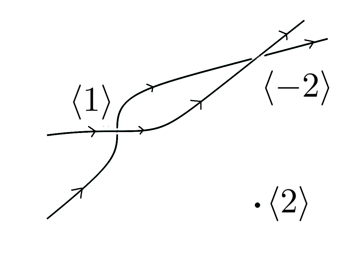
Figure 3. The quartic curve considered in 6.4 projected from the point $P$. The nodes of this planar curve correspond to secant lines containing $P$ and we denoted their local writhe in the picture.

If the theta characteristic $\alpha$ does not have global sections, then we can compute the arithmetic writhe of $C$ directly from the Ulrich bundle constructed in Section 5.5.

Theorem 6.5.

Let $L$ be a $3$-very ample line bundle on the curve $C$ and $\alpha$ a theta characteristic of $C$ with $h^{0}(C,\alpha)=0$. There exists a symmetric matrix $\Lambda$ whose entries are linear forms on $\wedge^{4}H^{0}(C,L)$ such that for all $s_{0}\ldots,s_{3}\in H^{0}(C,L)$ it holds that:

1. $\Lambda(s_{0}\wedge\cdots\wedge s_{3})$ is nonsingular if and only if the linear system spanned by the $s_{0},\ldots,s_{3}$ is very ample.

2. If the linear system spanned by the $s_{0},\ldots,s_{3}$ is very ample, then the writhe $\operatorname{w}(\psi(C),\alpha)$ is the class of $\Lambda(s_{0}\wedge\cdots\wedge s_{3})$ where $\psi\colon C\to\mathbb{P}^{3}$ is the embedding defined by $s_{0},\ldots,s_{3}$.

Proof.

Let $\Sigma$ the secant variety of $C$ embedded to $\mathbb{P}(H^{0}(C,L)^{\vee})$. Then the linear system spanned by $s_{0},\ldots,s_{3}\in H^{0}(C,L)$ is very ample if and only if $s_{0},\ldots,s_{3}$ do not have a common zero on $\Sigma$. If so, then $\operatorname{w}(\psi(C),\alpha)$ is the ${\mathbb{A}}^{1}$-degree of the linear projection $\Sigma\to\mathbb{P}^{3}$ given by $s_{0},\ldots,s_{3}$ restricted to the preimage of $\mathbb{P}^{3}\setminus C$ relatively oriented by the rank one symmetric Ulrich sheaf from 5.15. Hence the claim follows from 4.32. ∎

We end this section with some thoughts on whether every class $w\in\operatorname{GW}(K)$ can be realized as the writhe of a spatial curve.

Proposition 6.6.

For every $w\in\operatorname{GW}(K)$ with $\dim(w)=3$, there is a rational curve $X\subset\mathbb{P}^{3}$ of degree four with $\operatorname{w}(X)=w$.

Proof.

Let $C=\mathbb{P}^{1}$, $L={\mathcal{O}}_{\mathbb{P}^{1}}(4)$ and $\alpha={\mathcal{O}}_{\mathbb{P}^{1}}(-1)$. The matrix $\Lambda$ from 6.5 is then given by the Hankel matrix

$$\Lambda=\begin{pmatrix}x_{0}&x_{1}&x_{2}\\ x_{1}&x_{2}&x_{3}\\ x_{2}&x_{3}&x_{4}\end{pmatrix}$$

where $x_{i}$ denotes the linear form

$$f\mapsto f\wedge(r^{4-i}s^{i})\in\wedge^{5}K[r,s]_{4}=K$$

on $\wedge^{4}K[r,s]_{4}$. On the other hand, for arbitrary $a,b,c\in K^{\times}$ we have

$$\begin{pmatrix}a+\frac{b^{2}}{c}&0&b\\ 0&b&0\\ b&0&c\end{pmatrix}\cong\langle a\rangle+\langle b\rangle+\langle c\rangle.$$

Therefore, for every $w\in\operatorname{GW}(K)$ with $\dim(w)=3$, there is a rational curve $X\subset\mathbb{P}^{3}$ of degree four with $\operatorname{w}(X)=w$. ∎

Example 6.7.

We have for instance

$$\Lambda(r^{4}\wedge r^{3}s\wedge rs^{3}\wedge s^{4})=\begin{pmatrix}0&0&1\\ 0&1&0\\ 1&0&0\end{pmatrix}\cong 2\cdot\langle 1\rangle+\langle-1\rangle$$

which confirms our calculations from 6.4.

Question 1.

Let $d\in{\mathbb{N}}$ and $w\in\operatorname{GW}(K)$ with $\dim(w)=\frac{1}{2}(d-1)(d-2)$. Is there a rational curve $X\subset\mathbb{P}^{3}$ of degree $d$ with $\operatorname{w}(X)=w$? More generally, for any $w\in\operatorname{GW}(K)$ does there exist a curve $X\subset\mathbb{P}^{3}$ and a theta characteristic $\alpha$ on $X$ with $\operatorname{w}(X,\alpha)=w$?

Acknowledgements. We would like to thank the organizers of the Thematic Einstein Semester on “Algebraic Geometry: Varieties, Polyhedra, Computation” during which this project was initiated. We further thank Stephen McKean and Kirsten Wickelgren for helpful comments on a preliminary version of this manuscript.

References

• [Ago23] Daniele Agostini. The Martens–Mumford theorem and the Green–Lazarsfeld secant conjecture. J. Algebr. Geom., 2023. to appear, arXiv preprint arXiv:2110.03561.
• [AM11] Aravind Asok and Fabien Morel. Smooth varieties up to $\mathbb{A}^{1}$-homotopy and algebraic $h$-cobordisms. Adv. Math., 227(5):1990–2058, 2011.
• [Bea18] Arnaud Beauville. An introduction to Ulrich bundles. Eur. J. Math., 4(1):26–36, 2018.
• [Caz12] Christophe Cazanave. Algebraic homotopy classes of rational functions. Ann. Sci. Éc. Norm. Supér. (4), 45(4):511–534, 2012.
• [Eis05] David Eisenbud. The geometry of syzygies. A second course in commutative algebra and algebraic geometry, volume 229 of Grad. Texts Math. New York, NY: Springer, 2005.
• [ENP20] Lawrence Ein, Wenbo Niu, and Jinhyung Park. Singularities and syzygies of secant varieties of nonsingular projective curves. Invent. Math., 222(2):615–665, 2020.
• [ENP21] Lawrence Ein, Wenbo Niu, and Jinhyung Park. On blowup of secant varieties of curves. Electron Res. Arch., 29(6):3649–3654, 2021.
• [ES03] David Eisenbud and Frank-Olaf Schreyer. Resultants and Chow forms via exterior syzygies. Appendix by Jerzy Weyman: Homomorphisms and extensions between the bundles $\bigwedge^{p}U$ on the Grassmannian. J. Am. Math. Soc., 16(3):537–575, appendix 576–579, 2003.
• [Gey77] Wulf-Dieter Geyer. Reelle algebraische Funktionen mit vorgegebenen Null- und Polstellen. Manuscr. Math., 22:87–103, 1977.
• [GS] Daniel R. Grayson and Michael E. Stillman. Macaulay2, a software system for research in algebraic geometry. Available at http://www.math.uiuc.edu/Macaulay2/.
• [Har83] Robin Hartshorne. Algebraic geometry. Corr. 3rd printing, volume 52 of Grad. Texts Math. Springer, Cham, 1983.
• [HK23] Christoph Hanselka and Mario Kummer. Positive Ulrich sheaves. Canad. J. Math., published online:  http://dx.doi.org/10.4153/S0008414X23000263, 2023.
• [Huy06] Daniel Huybrechts. Fourier-Mukai transforms in algebraic geometry. Oxford Math. Monogr. Oxford: Clarendon Press, 2006.
• [KLSW23] Jesse Leo Kass, Marc Levine, Jake P. Solomon, and Kirsten Wickelgren. A quadratically enriched count of rational curves, 2023.
• [Kru18] Andreas Krug. Remarks on the derived McKay correspondence for Hilbert schemes of points and tautological bundles. Math. Ann., 371(1-2):461–486, 2018.
• [KS20] Mario Kummer and Eli Shamovich. Real fibered morphisms and Ulrich sheaves. J. Algebr. Geom., 29(1):167–198, 2020.
• [Kum16] Mario Kummer. From Hyperbolic Polynomials to Real Fibered Morphisms. PhD thesis, Universität Konstanz, Konstanz, 2016.
• [KW19] Jesse Leo Kass and Kirsten Wickelgren. The class of Eisenbud-Khimshiashvili-Levine is the local $\mathbb{A}^{1}$-Brouwer degree. Duke Math. J., 168(3):429–469, 2019.
• [KW21] Jesse Leo Kass and Kirsten Wickelgren. An arithmetic count of the lines on a smooth cubic surface. Compos. Math., 157(4):677–709, 2021.
• [Lev19] Marc Levine. Motivic Euler characteristics and Witt-valued characteristic classes. Nagoya Math. J., 236:251–310, 2019.
• [Lev20] Marc Levine. Aspects of enumerative geometry with quadratic forms. Doc. Math., 25:2179–2239, 2020.
• [McK21] Stephen McKean. An arithmetic enrichment of Bézout’s theorem. Math. Ann., 379(1-2):633–660, 2021.
• [MO19] Grigory Mikhalkin and Stepan Orevkov. Maximally writhed real algebraic links. Invent. Math., 216(1):125–152, 2019.
• [Mor06] Fabien Morel. $\mathbb{A}^{1}$-algebraic topology. In Proceedings of the international congress of mathematicians (ICM), Madrid, Spain, August 22–30, 2006. Volume II: Invited lectures, pages 1035–1059. Zürich: European Mathematical Society (EMS), 2006.
• [Mor12] Fabien Morel. $\mathbb{A}^{1}$-algebraic topology over a field, volume 2052 of Lect. Notes Math. Berlin: Springer, 2012.
• [MV99] Fabien Morel and Vladimir Voevodsky. $\mathbb{A}^{1}$-homotopy theory of schemes. Publ. Math., Inst. Hautes Étud. Sci., 90:45–143, 1999.
• [PW21] Sabrina Pauli and Kirsten Wickelgren. Applications to $\mathbb{A}^{1}$-enumerative geometry of the $\mathbb{A}^{1}$-degree. Res. Math. Sci., 8(2):29, 2021. Id/No 24.
• [Ull16] Brooke Ullery. On the normality of secant varieties. Adv. Math., 288:631–647, 2016.
• [Vir01] Oleg Viro. Encomplexing the writhe. In Topology, ergodic theory, real algebraic geometry. Rokhlin’s memorial, pages 241–256. Providence, RI: American Mathematical Society (AMS), 2001.