Source-Free Domain Adaptation with Temporal Imputation for Time Series Data

Abstract.

Source-free domain adaptation (SFDA) aims to adapt a pretrained model from a labeled source domain to an unlabeled target domain without access to the source domain data, preserving source domain privacy. Despite its prevalence in visual applications, SFDA is largely unexplored in time series applications. The existing SFDA methods that are mainly designed for visual applications may fail to handle the temporal dynamics in time series, leading to impaired adaptation performance. To address this challenge, this paper presents a simple yet effective approach for source-free domain adaptation on time series data, namely MAsk and imPUte (MAPU). First, to capture temporal information of the source domain, our method performs random masking on the time series signals while leveraging a novel temporal imputer to recover the original signal from a masked version in the embedding space. Second, in the adaptation step, the imputer network is leveraged to guide the target model to produce target features that are temporally consistent with the source features. To this end, our MAPU can explicitly account for temporal dependency during the adaptation while avoiding the imputation in the noisy input space. Our method is the first to handle temporal consistency in SFDA for time series data and can be seamlessly equipped with other existing SFDA methods. Extensive experiments conducted on three real-world time series datasets demonstrate that our MAPU achieves significant performance gain over existing methods. Our code is available at https://github.com/mohamedr002/MAPU_SFDA_TS.

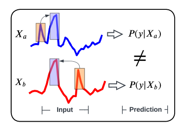
Figure 1. How do the temporal relations matter in time series? Despite similarities in the values of the two signals, variations in the temporal position of their observations can result in different predictions.

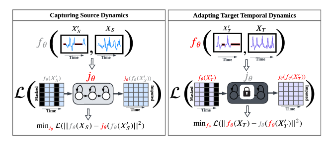
Figure 2. Adaptation with Temporal Imputation. Left: A temporal imputer network is trained to predict the full sequence from its masked version to capture the temporal information of the source domain. Right: Once trained, the temporal imputer network guides the target model to produce features that are temporally consistent with the source domain. (Best in viewed in colors. Components in red color are trainable, while those in gray color are non-trainable).

1. Introduction

Deep learning has achieved impressive performance in numerous time series applications, such as machine health monitoring, human activity recognition, and healthcare. However, this success heavily relies on the laborious annotation of large amounts of data. To address this issue, unsupervised domain adaptation (UDA) has gained traction as a way to leverage pre-labeled source data for training on unlabeled target data, while also addressing the distribution shift between the two domains (Wilson and Cook, 2020). There is a growing interest in applying UDA to time series data (Ragab et al., 2023), with existing methods seeking to minimize statistical distance across the source and target features (Zhu et al., 2021; Cai et al., 2021) or using adversarial training to find domain invariant features (Wilson et al., 2020, 2021; Jin et al., 2022; Ragab et al., 2022). However, these approaches require access to the source data during the adaptation process, which may not be always possible, due to data privacy regulations.

To address this limitation, a more practical setting, i.e., source-free domain adaptation (SFDA), has been proposed, where only a source-pretrained model is available during the adaptation process (Kim et al., 2021). In recent years, several SFDA methods have been developed for visual applications (Liang et al., 2020; Kim et al., 2021; Kothandaraman et al., 2021; Sahoo et al., 2020; Qiu et al., 2021). One prevalent paradigm has incorporated some auxiliary tasks to exploit the characteristics of visual data to improve the source-free adaptation (Liang et al., 2021; Bucci et al., 2021; Kothandaraman et al., 2021). However, all these methods are primarily designed for visual applications and may fail to handle the temporal dynamics of time series data.

In time series data, temporal dependency refers to the interdependence between values at different time points, which has a significant impact on predictions (Tonekaboni et al., 2020). As demonstrated in Figure 1, even two signals with similar observations can lead to differing predictions if the temporal order is different. Such temporal dynamics make adapting the temporal information between two shifted domains a key challenge in unsupervised domain adaptation. The problem becomes even more challenging under source-free adaptation settings, where no access to the source data is provided during the target adaptation. Therefore, our key question is how to effectively adapt temporal information in time series data in the absence of the source data.

In this work, we address the above challenges and propose a novel SFDA approach, i.e., MAsk and imPUte (MAPU), for time series data. Our method trains an autoregressive model to capture the temporal information on the source domain, which is then transferred to the target domain for adaptation. The key steps of our approach are illustrated in Figure 2. First, the input signal undergoes temporal masking. Both the masked signal and the original signal are then fed into an encoder network, which generates the corresponding feature representation. Subsequently, the temporal imputation network is trained to impute the original signal from the masked signal in the feature space, enabling smoother optimization for the temporal imputation task. During adaptation, the imputation network is used to guide the target model to generate target features that can be imputed by the source imputation network. Our method is versatile and can be integrated with the existing SFDA methods to provide them with temporal adaptation capability. The main contributions of this work can be summarized as follows:

• To the best of our knowledge, we are the first to achieve the source-free domain adaptation for time series applications.

• We propose a novel temporal imputation task to ensure sequence consistency between the source and target domains.

• We propose a versatile methodology for integrating temporal adaptation capability into existing SFDA methods.

• We conduct extensive experiments and demonstrate that our approach results in a significant improvement in adaptation performance on real-world data, and is particularly effective for time series adaptation tasks.

2. Related work

2.1. Time series Domain Adaptation

Several methods have been proposed to address the challenge of distribution shift in time series data. These methods can be broadly categorized into two groups: discrepancy-based methods and adversarial-based methods. Discrepancy-based methods use statistical distances to align the feature representations of the source and target domains. For instance, AdvSKM leverages the maximum mean discrepancy (MMD) distance in combination with a hybrid spectral kernel to consider temporal dependencies during domain adaptation (Liu and Xue, 2021). Another example is SASA, which learns the association structure of time series data to align the source and target domains (Cai et al., 2021). On the contrary, adversarial-based methods use adversarial training to mitigate the distribution shift between the source and target domains. For instance, CoDATS utilizes a gradient reversal layer (GRL) for adversarial training with weak supervision on multi-source human activity recognition data (Wilson et al., 2020). Furthermore, DA_ATTN couples adversarial training with an un-shared attention mechanism to preserve the domain-specific information (Jin et al., 2022). Recently, SLARDA presents an autoregressive adversarial training approach for aligning temporal dynamics across domains (Ragab et al., 2022).

Albeit promising, the design of these methods is based on the assumption that source data is available during the adaptation step. However, accessing source data may not be possible in practical situations due to privacy concerns or storage limitations. Differently, our MAPU adapts a model pretrained on source data to new domains without access to source data during adaptation, which can be a more practical solution for high-stake applications.

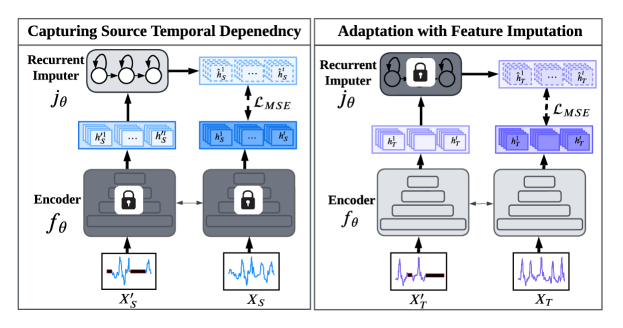
Figure 3. Adaptation with Temporal Imputation for time series data. Left: The pretraining stage of the temporal imputer network $j_{\theta}$ to capture the temporal dynamics of the source domain. First, we perform random masking across the time dimension of the source signal. Given the original source signal $X_{S}$ and its temporally masked signal $X_{S}^{\prime}$, the encoder network $f_{\theta}$ is used to generate the corresponding latent features $H_{S}$ and $H_{S}^{\prime}$ respectively. Subsequently, $j_{\theta}$ is updated to produce imputed features $\hat{H}_{S}$ from masked features $H_{S}^{\prime}$ using the mean square error loss. Right: The adaptation stage of the encoder network on the target domain data. The encoder $f_{\theta}$ is updated to produce source-like features that are imputable by the pretrained $j_{\theta}$.

2.2. Source Free Domain Adaptation

Source-Free Domain Adaptation (SFDA) is a new problem-setting, where we do not have access to the source domain data during adaptation. This objective can be achieved in several ways. One approach is to leverage a model pretrained on the source domain to generate synthetic source-like data during the adaptation step (Qiu et al., 2021; Li et al., 2020; Kurmi et al., 2021; Sahoo et al., 2020). Another approach is to use adversarial training between multiple classifiers to generalize well to the target classes (Chu et al., 2022a; Xia et al., 2021). Another prevalent approach uses softmax scores or their corresponding entropy to prioritize confident samples for pseudo-labeling, assuming that the model should be more confident on source samples and less confident on target samples (Liang et al., 2020; Kim et al., 2021; Kothandaraman et al., 2021).

Despite the strong potential demonstrated by these methods, they are primarily designed for visual applications and may fail to effectively align temporal dynamics in time series data. In contrast, our method addresses this challenge through a novel temporal imputation task, ensuring temporal consistency between domains during the adaptation.

3. Methodology

3.1. Problem definition

Given a labeled source domain $\mathcal{D}_{S}=\{{X}_{S}^{i},{y}_{S}^{i}\}_{i=1}^{n_{S}}$, where ${X}_{S}\in\mathcal{X}_{S}$ can be a uni-variate or multi-variate time series data with a sequence length $L$, while $y_{S}\in\mathcal{Y}_{S}$ represents the corresponding labels. In addition, we have an unlabeled target domain $\mathcal{D}_{T}=\{{X}_{T}^{i}\}_{i=1}^{n_{T}}$, where ${X}_{T}\in\mathcal{X}_{T}$, and it also shares the same label space with $\mathcal{D}_{S}$. Following the existing UDA settings, we assume a difference across the marginal distributions, i.e., $P(X_{S})\neq P(X_{T})$, while the conditional distributions are stable, i.e., $P(y_{S}|X_{S})\approx P(y_{T}|X_{T})$.

This work aims to address the source-free domain adaptation problem, where access to source data is strictly prohibited during the adaptation phase to ensure data privacy. Furthermore, we adopt the vendor-client source-free paradigm (Kundu et al., 2022b, 2020; Chu et al., 2022b; Kundu et al., 2022a), which allows the influence of the source pretraining stage. This assumption is realistic in use cases where there is a collaboration between various entities, but it is not possible to share source data due to data privacy, security, or regulatory issues.

3.2. Overview

We present our MAPU to achieve source-free adaptation on time series temporal data while considering the temporal dependencies across domains. The pipeline of the proposed method is illustrated in Figure 4. Given the input signal and a temporally masking signal, our method comprises two stages: (1) training an autoregressive network, referred to as the imputer network, which captures the temporal information of the source domain through a novel temporal imputation task, and (2) leveraging the source-pretrained imputer network to guide the target encoder towards producing temporally consistent target features in the adaptation stage. Next, we will first elaborate on the temporal masking procedure before delving into the details of each stage.

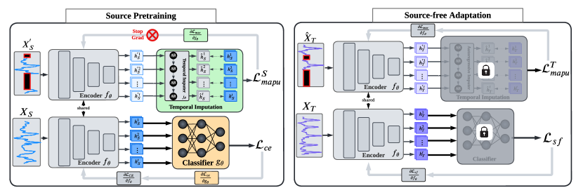
Figure 4. Integrating our temporal imputation with other source-free methods (Best viewed in colors). Left: In the pretraining stage, the source model is trained using conventional cross-entropy loss $\mathcal{L}_{ce}$, and the temporal imputer network is trained using $\mathcal{L}_{mapu}^{S}$ to impute the features of the masked signals and capture the source temporal information on the feature space. Right: In the adaptation stage, the target model is jointly trained with both a generic source-free adaptation loss $\mathcal{L}_{sf}$ and our temporal imputation loss $\mathcal{L}_{mapu}^{T}$ to perform the adaptation while ensuring temporal consistency with the source features.

3.3. Temporal Masking

In this section, we explain our process of temporal masking. We start by dividing the input signal, $X$, into several blocks along the time dimension. Then, we randomly choose some of these blocks and set their values to zero, creating a masked version of the signal called $X^{\prime}$. This process is applied to both the source and target domains. Our aim is to challenge the model to use the information from surrounding blocks to fill in the missing parts and capture the temporal dependencies in the input signal. Further discussion on the impact of the masking ratio on the adaptation performance can be found in the experiment section.

3.4. Capturing Source Temporal Dynamics

In the pretraining stage, current methods typically map the source data from the input space to the feature space using an encoder network, represented as $f_{\theta}:\mathcal{X}_{S}\rightarrow\mathcal{H}_{S}$. The extracted features are then passed through a classifier network, $g_{\theta}:\mathcal{H}_{S}\rightarrow\mathcal{Y}_{S}$, to make class predictions for the source data. However, to effectively adapt to other time series domains, it is important to consider the temporal relations in the source domain. Using only cross-entropy for training the source network may neglect this aspect. To address this, we propose a temporal imputation task that aims to recover the input signal from a temporally masked signal in the feature space.

The imputation task is performed by an imputer network $j_{\theta}$ that takes the masked signal and maps it to the original signal. The input signal $X_{S}$ and masked signal $X_{S}^{\prime}$ are first transformed into their corresponding feature representations $H_{S}$ and $H_{S}^{\prime}$ by the encoder $f_{\theta}$. The task of the imputer network is represented as $\hat{H}_{S}^{\prime}=j_{\theta}(f_{\theta}(X_{S}^{\prime}))\rightarrow H_{S}=f_{\theta}(X_{S})$, where $\hat{H}_{S}^{\prime}$ is the imputed signal. The imputer network is trained to minimize the mean square error between the features of the original signal and the imputed signal, which can be formulated as:

(1) $$\min_{j_{\theta}}\mathcal{L}_{mapu}^{S}=\frac{1}{n}\sum_{i=1}^{n_{S}}\left\|f_{\theta}(X_{S}^{i})-j_{\theta}(f_{\theta}(X_{S}^{\prime i}))\right\|_{2}^{2},$$

where $H_{S}=f_{\theta}(X_{S}^{i})$ are the latent features of the original signal, $\hat{H}_{S}=j_{\theta}(f_{\theta}(X_{S}^{\prime i}))$ is the output of the imputer network, and $n_{S}$ is the total number of source samples.

3.5. Temporal Adaptation with Feature Imputation

In the adaptation stage, the goal is to train the target encoder network to produce target features temporally consistent with the source features. The target encoder network $f_{\theta}$ is used to extract latent feature representations from a target sample $X_{T}$ and its masked version $X_{T}^{\prime}$. The fixed source-pretrained imputer network $j_{\theta}$ is then used to reconstruct the features of the original signal from the masked features. However, due to domain differences, the source imputer may not be able to accurately reconstruct the target features. Thus, the encoder network $f_{\theta}$ is updated to produce target features that can be accurately reconstructed by the imputer network. This can be expressed as the following optimization problem:

(2) $$\min_{f_{\theta}}\mathcal{L}_{mapu}^{T}=\frac{1}{n}\sum_{i=1}^{n_{T}}\left\|f_{\theta}(X_{T})^{i}-j_{\theta}(f_{\theta}(X_{T}^{\prime})^{i}))\right\|_{2}^{2},$$

where $H_{T}=f_{\theta}(X_{T})$ are the original target features, $\hat{H}_{T}=j_{\theta}(f_{\theta}(X_{T}^{\prime}))$ are the adapted target features produced by the imputer network to minimize the mean square error loss, and $n_{T}$ is the total number of target samples. Notably, only the encoder network is optimized, producing features that can be accurately imputed by the fixed source-pretrained imputer network. To reduce the imputation loss, the adapted target features should be temporally consistent with the source features.

Algorithm 1 illustrates the adaptation procedure via temporal imputation. The process starts by first constructing a temporally masked version of the input target sample represented as $X_{T}^{\prime}$. Next, the source-pretrained encoder is used to extract the latent features of both the original signal and the temporally masked signal, represented as $H_{T}$ and $H_{T}^{\prime}$, respectively. Finally, the encoder network is updated to make features of the masked signal recoverable by the source-pretrained imputer network, using the mean square error loss in Equation 2.

Algorithm 1 Adaptation with Temporal Imputation

1:Input: Target sample $X_{T}$, source pretrained encoder $f_{\theta}$, source classifier $g_{\theta}$, imputer network $j_{\theta}$

2:Initialize: Construct temporally masked version of $X_{T}$: $X_{T}^{\prime}$

3:Extract: Latent feature representations: $H_{T}=f_{\theta}(X_{T})$, $H_{T}^{\prime}=f_{\theta}(X_{T}^{\prime})$

4:Impute: Masked features using imputer network: $\hat{H}_{T}=j_{\theta}(H_{T}^{\prime})$

5:Update: Encoder $f_{\theta}$ to produce target features that can be accurately reconstructed by $j_{\theta}$ using Equation 2

6:Output: Updated encoder $f_{\theta}$

3.6. Integration with Other Source-free Methods

Our proposed MAPU is generic and can be integrated with other source-free adaptation methods. Typically, source-free adaptation involves a two-stage training procedure: (1) pretraining the source model with source domain data, and (2) adapting the pretrained model to the target domain. As shown in Figure 4, our MAPU can be seamlessly integrated into existing SFDA methods in both stages.

In the pretraining stage, MAPU operates in the feature space by training the temporal imputation network, $j_{\theta}$, to capture the temporal information from the source domain. The loss associated with the temporal imputation task does not propagate to the encoder model, $f_{\theta}$. As a result, the encoder can be trained exclusively with the conventional cross-entropy loss, ensuring that the imputation task does not negatively impact the pretraining performance. The total pretraining loss is formalized as:

(3) $$\min_{f_{\theta},j_{\theta}}\mathcal{L}_{\mathrm{S}}=-\mathbb{E}_{({X}_{S},y_{S})\sim\mathcal{D}_{S}}\mathcal{L}_{\mathrm{ce}}+\mathcal{L}_{\mathrm{mapu}}^{S},$$

where $\mathcal{L}_{\mathrm{ce}}=\sum_{k=1}^{K}\mathbbm{1}_{[y_{S}=k]}\log(\hat{p}_{k})$ represents the standard cross-entropy loss between the predicted label and the true label, $\hat{p}k^{i}$ represents the predicted probability for class $k$ and sample $i$, and $\mathcal{L}_{\mathrm{mapu}}^{S}$ represents the training loss for our temporal imputer network on the source data to capture the source temporal information.

In the target adaptation step, the objective is to optimize the target encoder, $f_{\theta}$, by balancing the temporal imputation loss and the generic source-free loss to achieve temporal consistency and perform adaptation on the target domain. This can be formalized as follows:

(4) $$\min_{f_{\theta}}L_{T}=\mathbb{E}_{{X}_{T}\sim\mathcal{D}_{T}}\mathcal{L}_{sf}+\alpha\mathcal{L}_{mapu}^{T},$$

where $\alpha$ is a hyperparameter that regulates the relative importance of the temporal imputation task, and $\mathcal{L}_{sf}$ represents the generic loss used by the SFDA method to adapt the target domain to the source domain.

4. Experimental Settings

4.1. Datasets

We evaluate our proposed method on three real-world datasets spanning three time series applications, i.e., machine fault diagnosis, human activity recognition, and sleep stage classification. The selected datasets differ in many aspects, as illustrated in Table 4.1.3, which leads to a considerable domain shift across different domains.

4.1.1. UCIHAR Dataset

This dataset focuses on human activity recognition tasks. Three types of sensors have been used to collect the data, i.e., accelerator sensor, gyroscope sensor, and body sensor, where each sensor provides three-dimensional readings, leading to a total of 9 channels per sample, with each sample containing 128 data points. The data is collected from 30 different users and each user is considered as one domain. In our experiments, five cross-user experiments are conducted, where the model is trained on one user and tested on different users to evaluate its cross-domain performance (Anguita et al., 2013).

4.1.2. Sleep Stage Classification (SSC) Dataset

The Sleep Stage Classification (SSC) task involves categorizing Electroencephalography (EEG) signals into five distinct stages, namely Wake (W), Non-Rapid Eye Movement stages (N1, N2, N3), and Rapid Eye Movement (REM). To accomplish this, we utilize the Sleep-EDF dataset (Goldberger et al., 2000), which comprises EEG readings from 20 healthy subjects. In line with previous studies (Eldele et al., 2021a), we select a single channel, specifically Fpz-Cz, and utilize 10 subjects to construct five cross-domain experiments.

4.1.3. Machine Fault Diagnosis (MFD) Dataset

This dataset has been collected by Paderborn university for the fault diagnosis application, where the vibration signals are leveraged to identify different types of incipient faults. The data has been collected under four different working conditions. Each data sample consists of a single univariate channel and 5120 data points following previous works (Lessmeier et al., 2016; Ragab et al., 2022). In our experiments, each working condition is considered as one domain, where we utilize five different cross-condition scenarios to evaluate the domain adaptation performance.

More details about the datasets are included in Table 4.1.3.

Table 1. Details of the adopted datasets (C: #channels, K: #classes, L: sample length).

l—ccc—cc Dataset C K L # training samples # testing samples

UCIHAR 9 6 128 2300 990
SSC 1 5 3000 14280 6130
MFD 1 3 5120 7312 3604

Table 2. Detailed results of the five UCIHAR cross-domain scenarios in terms of MF1 score.

@l—c—ccccc—c@ Algorithm SF 2$\rightarrow$11 12$\rightarrow$16 9$\rightarrow$18 6$\rightarrow$23 7$\rightarrow$13 AVG
DDC ✗ 60.0$\pm$13.32 66.77$\pm$8.46 61.41$\pm$5.80 88.55$\pm$1.42 77.29$\pm$2.11 75.67
DCoral ✗ 67.2$\pm$13.67 64.58$\pm$8.72 54.38$\pm$9.69 89.66$\pm$2.54 90.46$\pm$2.96 77.71
HoMM ✗ 83.54$\pm$2.99 63.45$\pm$2.07 71.25$\pm$4.42 94.97$\pm$2.49 91.41$\pm$1.33 84.10

MMDA ✗ 72.91$\pm$2.78 74.64$\pm$2.88 62.62$\pm$2.63 91.14$\pm$0.46 90.61$\pm$2.00 81.40

DANN ✗ 98.09$\pm$1.68 62.08$\pm$1.69 70.7$\pm$11.36 85.6$\pm$15.71 93.33$\pm$0.00 84.97

CDAN ✗ 98.19$\pm$1.57 61.20$\pm$3.27 71.3$\pm$14.64 96.73$\pm$0.00 93.33$\pm$0.00 86.79

CoDATS ✗ 86.65$\pm$4.28 61.03$\pm$2.33 80.51$\pm$8.47 92.08$\pm$4.39 92.61$\pm$0.51 85.47

AdvSKM ✗ 65.74$\pm$2.69 60.52$\pm$1.99 53.25$\pm$5.19 79.63$\pm$8.52 88.89$\pm$3.12 74.67

SHOT ✓100.0$\pm$0.00 70.76$\pm$6.22 70.19$\pm$8.99 98.91$\pm$1.89 93.01$\pm$0.57 86.57
NRC ✓ 97.02$\pm$2.82 72.18$\pm$0.59 63.10$\pm$4.84 96.41$\pm$1.33 89.13$\pm$0.54 83.57
AaD ✓ 98.51$\pm$2.58 66.15$\pm$6.15 68.33$\pm$11.9 98.07$\pm$1.71 89.41$\pm$2.86 84.09
MAPU ✓ 100.0$\pm$0.00 67.96$\pm$4.62 82.77$\pm$2.54 97.82$\pm$1.89 99.29$\pm$1.22 89.57

4.2. Implementation Details

Encoder Design

In our study, we adopt the encoder architecture presented in existing works (Ragab et al., 2023; Eldele et al., 2021b), which is a 1-dimensional convolutional neural network composed of three layers with filter sizes of 64, 128, and 128 respectively. Each conventional layer was followed by the application of a rectified linear unit activation function and batch normalization.

MAPU Parameters

For the purpose of temporal masking, a masking ratio of 1/8 is utilized across all datasets in our experiments. To perform the imputation task, a single-layer recurrent neural network with a hidden dimension of 128 is employed for all datasets. In addition, our method includes a primary hyperparameter, $\alpha$, which is set to 0.5 for all datasets in our evaluation.

Unified Training Scheme

To provide a fair and valid comparison with source-free baseline methods, we adhered to their established implementations (Liang et al., 2020; Yang et al., 2021, 2022) while incorporating the same backbone network and training procedures utilized in our proposed method. In accordance with the AdaTime framework (Ragab et al., 2023), all the models are trained for a total of 40 epochs, using a batch size of 32, with a learning rate of 1e-3 for UCIHAR and 1e-4 for SSC and MFD. Also, the macro F1-score (MF1) metric (Ragab et al., 2023) has been used to ensure a reliable evaluation under data imbalance situations, where we report the mean and the standard deviation of three consecutive runs for each cross-domain scenario.

4.3. Baseline Methods

To evaluate the performance of our model, we compare it against conventional UDA approaches that assume access to source data during adaptation. These baselines are adapted from the AdaTime benchmark (Ragab et al., 2023). Additionally, we compare our model against recent source-free domain adaptation methods. To ensure fair evaluation, we re-implement all source-free baselines in our framework, while ensuring the same backbone network and training schemes. Overall the compared methods are as follows:

Conventional UDA methods

• Deep Domain Confusion (DDC) (Tzeng et al., 2014): leverages the MMD distance to align the source and target features.

• Deep Correlation Alignment (DCORAL) (Sun et al., 2017): aligns the second-order statistics of the source and target distributions in order to effectively minimize the shift between the two domains.

• High-order Maximum Mean Discrepancy (HoMM) (Chen et al., 2020): aligns the high-order moments to effectively tackle the discrepancy between the two domains.

• Minimum Discrepancy Estimation for Deep Domain Adaptation (MMDA) (Rahman et al., 2020): combines the MMD and correlation alignment with entropy minimization to effectively address the domain shift issue.

• Domain-Adversarial Training of Neural Networks (DANN) (Ganin et al., 2016): leverages gradient reversal layer to adversarially train a domain discriminator network against an encoder network.

• Conditional Domain Adversarial Network (CDAN) (Long et al., 2018): realizes a conditional adversarial alignment by integrating task-specific knowledge with the features during the alignment step for the different domains.

• Convolutional deep adaptation for time series (CoDATS) (Wilson et al., 2020): employs adversarial training with weak supervision to enhance the adaptation performance on time series data.

• Adversarial spectral kernel matching (AdvSKM)(Liu and Xue, 2021): introduces adversarial spectral kernel matching to tackle the challenges of non-stationarity and non-monotonicity present in time series data.

Source-free methods

• Source Hypothesis Transfer (SHOT) (Liang et al., 2020): minimizes information maximization loss with self-supervised pseudo labels to identify target features that can be compatible with the transferred source hypothesis.

• Exploiting the intrinsic neighborhood structure (NRC) (Yang et al., 2021): captures the intrinsic structure of the target data by forming clear clusters and encouraging label consistency among data with high local affinity.

• Attracting and dispersing (AaD) (Yang et al., 2022): optimizes an objective of prediction consistency by treating SFDA as an unsupervised clustering problem and encouraging local neighborhood features in feature space to have similar predictions.

Table 3. Detailed results of the five SSC cross-domain scenarios in terms of MF1 score.

l—c—ccccc—c Algorithm SF 16$\rightarrow$1 9$\rightarrow$14 12$\rightarrow$5 7$\rightarrow$18 0$\rightarrow$11 AVG
DDC ✗ 55.47$\pm$1.72 63.57$\pm$1.43 55.43$\pm$2.75 67.46$\pm$1.45 54.17$\pm$1.79 59.22

DCoral ✗ 55.50$\pm$1.74 63.50$\pm$1.36 55.35$\pm$2.64 67.49$\pm$1.50 53.76$\pm$1.89 59.12

HoMM ✗ 55.51$\pm$1.79 63.49$\pm$1.14 55.46$\pm$2.71 67.50$\pm$1.50 53.37$\pm$2.47 59.06

MMDA ✗ 62.92$\pm$0.96 71.04$\pm$2.39 65.11$\pm$1.08 70.95$\pm$0.82 43.23$\pm$4.31 62.79

DANN ✗ 58.68$\pm$3.29 64.29$\pm$1.08 64.65$\pm$1.83 69.54$\pm$3.00 44.13$\pm$5.84 60.26

CDAN ✗ 59.65$\pm$4.96 64.18$\pm$6.37 64.43$\pm$1.17 67.61$\pm$3.55 39.38$\pm$3.28 59.04
CoDATS ✗ 63.84$\pm$3.36 63.51$\pm$6.92 52.54$\pm$5.94 66.06$\pm$2.48 46.28$\pm$5.99 58.44
AdvSKM ✗ 57.83$\pm$1.42 64.76$\pm$3.00 55.73$\pm$1.42 67.58$\pm$3.64 55.19$\pm$4.19 60.21

SHOT ✓ 59.07$\pm$2.14 69.93$\pm$0.46 62.11$\pm$1.62 69.74$\pm$1.22 50.78$\pm$1.90 62.33
NRC ✓ 52.09$\pm$1.89 58.52$\pm$0.66 59.87$\pm$2.48 66.18$\pm$0.25 47.55$\pm$1.72 56.84
AaD ✓ 57.04$\pm$2.03 65.27$\pm$1.69 61.84$\pm$1.74 67.35$\pm$1.48 44.04$\pm$2.18 59.11
MAPU ✓ 63.85$\pm$4.63 74.73$\pm$0.64 64.08$\pm$2.21 74.21$\pm$0.58 43.36$\pm$5.49 64.05

Table 4. Detailed results of the five MFD cross-domain scenarios in terms of MF1 score.

@l—c—ccccc—c@ Algorithm SF 0$\rightarrow$1 1$\rightarrow$0 1$\rightarrow$2 2$\rightarrow$3 3$\rightarrow$1 AVG
DDC ✗ 74.50$\pm$5.56 48.91$\pm$6.24 89.34$\pm$2.16 96.34$\pm$3.07 100.0$\pm$0.00 81.82
DCoral ✗ 79.03$\pm$8.83 40.83$\pm$5.01 82.71$\pm$0.76 98.01$\pm$0.67 97.73$\pm$3.93 79.66
HoMM ✗ 80.80$\pm$2.46 42.31$\pm$5.90 84.28$\pm$1.32 98.61$\pm$0.08 96.28$\pm$6.45 80.46
MMDA ✗ 82.44$\pm$4.47 49.35$\pm$5.02 94.07$\pm$2.72 100.0$\pm$0.00 100.0$\pm$0.00 85.17
DANN ✗ 83.44$\pm$1.72 51.52$\pm$0.38 84.19$\pm$2.10 99.95$\pm$0.09 100.0$\pm$0.00 83.82
CDAN ✗ 84.97$\pm$0.62 52.39$\pm$0.49 85.96$\pm$0.90 99.7$\pm$0.45 100.0$\pm$0.00 84.60
CoDATS ✗ 67.42$\pm$13.3 49.92$\pm$13.7 89.05$\pm$4.73 99.21$\pm$0.79 99.92$\pm$0.14 81.10
AdvSKM ✗ 76.64$\pm$4.82 43.81$\pm$6.29 83.10$\pm$2.19 98.85$\pm$0.93 100.0$\pm$0.00 80.48

SHOT ✓ 41.99$\pm$2.78 57.00$\pm$0.09 80.70$\pm$1.49 99.48$\pm$0.31 99.95$\pm$0.05 75.82
NRC ✓ 73.99$\pm$1.36 74.88$\pm$8.81 69.23$\pm$0.75 78.04$\pm$11.3 71.48$\pm$4.59 73.52
AaD ✓ 71.72$\pm$3.96 75.33$\pm$4.65 78.31$\pm$2.26 90.07$\pm$7.02 87.45$\pm$11.7 80.58
MAPU ✓ 99.43$\pm$0.51 77.42$\pm$0.16 85.78$\pm$7.38 99.67$\pm$0.50 99.97$\pm$0.05 92.45

5. Results

In this section, we rigorously test our approach against state-of-the-art methods in various time series applications. We also assess the versatility of our method by combining it with different SFDA techniques. Furthermore, we compare the effectiveness of our task to other auxiliary tasks on time series data. Lastly, we examine our model’s sensitivity to different importance weights and masking ratios. In our MAPU, we leverage SHOT as the base SFDA method. Nevertheless, our approach is not limited to SHOT and can be effectively integrated with other SFDA methods, as demonstrated in our versatility experiments.

5.1. Quantative Results

To assess the efficacy of our approach, we evaluate its performance on three different time series datasets, namely, UCIHAR, SSC, and MFD. Tables 4.1.3, 4.3, and 4.3 present results for five cross-domain scenarios in each dataset, as well as an average performance across all scenarios (AVG). The algorithms are divided into two groups: the traditional UDA methods are marked with ✗, while the source-free methods are marked with ✓.

5.1.1. Evaluation on UCIHAR Dataset

The results presented in Table 4.1.3 show the performance of our MAPU in five cross-subject scenarios. Our method demonstrates superior performance in three of the five scenarios, achieving an overall performance of 89.57%. This exceeds the second-best source-free method by 3%. Notably, the source-free methods (i.e., SHOT, NRC, and AaD) perform competitively with conventional unsupervised domain adaptation (UDA) methods that utilize source data. This can be attributed to the two-stage training (i.e., pertaining and adaptation) scheme employed in the source-free methods, which focuses on optimizing the target model for the target domain without considering source performance (Qiu et al., 2021). Furthermore, our MAPU, with its temporal adaptation capability, outperforms all conventional UDA methods, surpassing the best method (i.e., CDAN) by 2.78%.

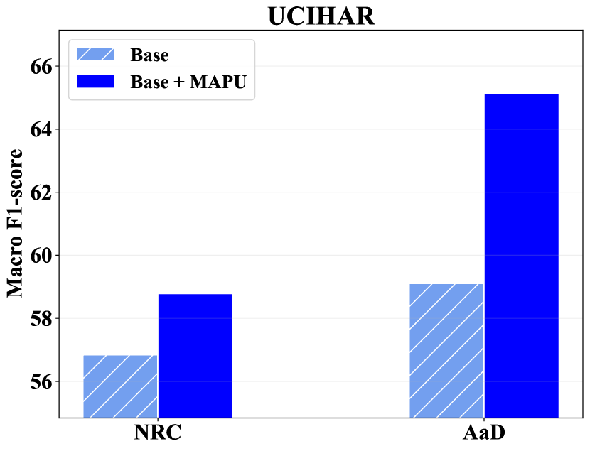
(a)

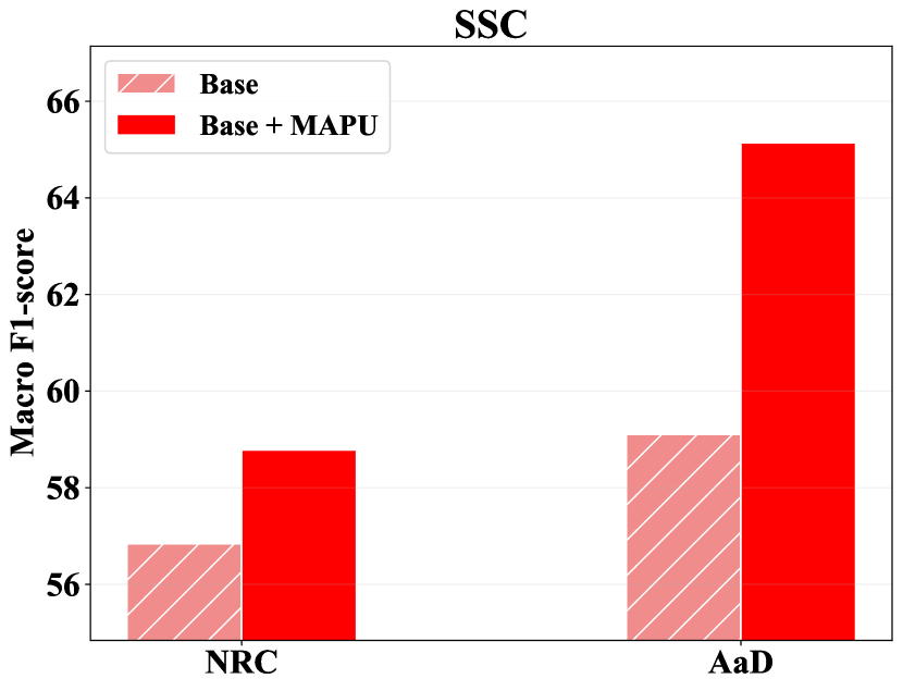
(b)

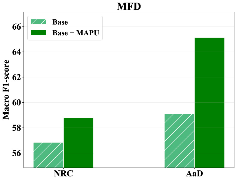
(c)

Figure 5. Intergrating temporal imputation with existing SFDA methods among the three datasets.

5.1.2. Evaluation on SSC Dataset

The results of the sleep stage classification task, as presented in Table 4.3, demonstrate the superior performance of our proposed method, MAPU, over other baseline methods. Our MAPU performs best in three out of the five cross-domain scenarios, with an overall performance of 64.05%. This is higher than the best source-free method, SHOT, and the best conventional UDA method, with an improvement of 1.72% and 1.27% respectively. It is worth noting that source-free methods that rely on features clustering, i.e., NRC and AaD, perform poorly on the SSC dataset due to its class-imbalanced nature. However, our MAPU, with its temporal adaptation capability, is able to handle such imbalance and outperform all source-free methods with a maximum improvement of 4.8% in scenario 16 $\rightarrow$1.

5.1.3. Evaluation on MFD Dataset

The results of the Machine Fault Diagnosis (MFD) task, presented in Table 4.3, showcase the superior performance of our MAPU when compared to all other baselines. With an average performance of 92.45%, MAPU exceeds the second-best method by a large margin of 7.85%. Additionally, MAPU significantly outperforms baseline methods in the hard transfer tasks (i.e., 0$\rightarrow$1 and 1$\rightarrow$0), reaching a 14.46% improvement in the latter scenario, while performing competitively with other baseline methods in the easy transfer tasks (i.e., $2\rightarrow 3$ and $3\rightarrow 1$). Compared to source-free methods, our MAPU achieves the best performance in all cross-domains, surpassing the second-best source-free method, AaD, by 11.87%.

It is worth noting that the performance improvement of our method is relatively large in the MFD dataset compared to other datasets. This is mainly attributed to two reasons. First, the MFD dataset has the longest sequence length among all other datasets, thus, the adaptation of temporal information is more prominent and necessary. Second, unlike other datasets, this dataset has a limited number of classes, i.e., 3 classes, and thus, failing to correctly classify one class can significantly harm the performance.

Table 5. Comparing the temporal imputation task with conventional auxiliary tasks for time series adaptation.

l—ccc Task UCIHAR SSC MFD
SHOT 86.57 62.33 75.82
SHOT+ Rotation 86.78 60.33 84.98
SHOT + Jigsaw 87.83 62.11 85.74
SHOT + Temporal 89.57 64.05 92.45

NRC 83.57 56.84 73.52
NRC+ Rotation 71.62 56.75 72.02
NRC + Jigsaw 70.58 56.91 74.68
NRC + Temporal 86.05 58.78 76.34
AaD 84.09 59.11 80.58
AaD + Rotation 71.52 59.00 84.18
AaD + Jigsaw 83.72 59.17 85.31
AaD + Temporal 87.00 64.05 91.11

5.2. Ablation Study on Auxiliary Tasks

To demonstrate the effectiveness of our proposed temporal imputation auxiliary task, we conducted evaluations using various auxiliary tasks, including rotation prediction (Liang et al., 2021) and jigsaw puzzle (Bucci et al., 2021). We chose three different SFDA backbones, SHOT, NRC, and AaD, for the auxiliary tasks to eliminate the bias to a specific SFDA method. Table 5.1.3 shows the average performance of five cross-domain scenarios for each dataset. The results show that our temporal imputation task consistently outperforms the other tasks across all datasets, even when combined with different SFDA backbones. Meanwhile, the baseline tasks, including rotation and jigsaw, not only exhibit limited improvement but also consistently harm the performance in many cases across various datasets. This indicates the inadequacy of these tasks for time series data and highlights the importance of considering temporal dynamics to the adaptation performance, as demonstrated by the superior performance of our MAPU approach.

5.3. Model Analysis

5.3.1. Versatility Analysis

This study investigates the effectiveness of incorporating temporal information into other SFDA methods. To achieve that, we evaluated the performance of three different SFDA methods when used in conjunction with our proposed temporal imputation task on the UCIHAR, SSC, and MFD datasets. Figure 5 shows the average performance of five cross-domain scenarios in each dataset. Our results indicate a significant improvement in performance across all tested datasets through the integration of our temporal imputation task. For instance, on the UCIHAR dataset, we saw a notable 3% boost in performance for the NRC and AaD methods. On the UCIHAR dataset, the NRC and AaD methods all experienced a performance boost of approximately 3% upon integration with our temporal imputation task. The improvements are consistent across the SSC and MFD datasets, demonstrating our approach’s effectiveness in providing temporal adaptation capability to existing SFDA methods that are mainly proposed for visual applications.

5.3.2. Sensitivity Analysis

This study evaluates the sensitivity of our temporal imputation component to the relative weight $\alpha$ when integrated with other SFDA methods, as illustrated in Figure 6. The results indicate that our model’s performance is relatively stable across a range of values for the $\alpha$ parameter. Particularly, the highest MF1 score achieved was 89.77, while the lowest accuracy was 87.75, with a difference of only 2%. This observed stability may be attributed to the imputation process being carried out on the feature space rather than the input space. As such, the feature space provides a more abstract representation of the data, making the imputation process free of the variations present in the input space.

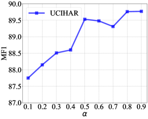
Figure 6. Analysis of adaptation performance with varying relative weight for the temporal imputation component $\alpha$.

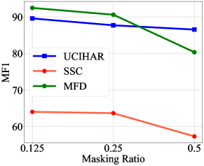
Figure 7. Effect of temporal masking ratio on the adaptation performance for the three datasets.

5.3.3. Impact of Masking level

Here, we systematically examine the impact of the masking ratio on adaptation performance in the context of imputation tasks. Specifically, we employed three different masking ratios (12.5%, 25%, and 50%) and evaluated the performance on the three benchmark datasets. The results, shown in Figure 7, reveal a clear trend of improved performance with lower masking ratios. Notably, the best performance was achieved with a masking ratio of 12.5% across all datasets. These findings suggest that excessive masking may negatively impact the adaptation performance in the imputation task.

6. Conclusion

This paper introduced MAsk And imPUte (MAPU), a novel method for source-free domain adaptation on time series data. The proposed method addressed the challenge of temporal consistency in time series data by proposing a temporal imputation task to recover the original signal in the feature space rather than the input space. MAPU is the first method to explicitly account for temporal dependency in a source-free manner for time series data. The effectiveness of MAPU is demonstrated through extensive experiments on three real-world datasets, achieving significant gains over the existing methods. This work highlights the potential of MAPU in addressing the domain-shift problem while preserving data privacy in time series applications.

7. Acknowledgments

This work was supported by the Agency of Science Technology and Research under its AME Programmatic (Grant No. A20H6b0151) and its Career Development Award (Grant No. C210112046).

References

- (1)
- Anguita et al. (2013) Davide Anguita, Alessandro Ghio, Luca Oneto, Xavier Parra, and Jorge Luis Reyes-Ortiz. 2013. A public domain dataset for human activity recognition using smartphones. In European Symposium on Artificial Neural Networks.
- Bucci et al. (2021) Silvia Bucci, Antonio D’Innocente, Yujun Liao, Fabio M Carlucci, Barbara Caputo, and Tatiana Tommasi. 2021. Self-supervised learning across domains. IEEE Transactions on Pattern Analysis and Machine Intelligence 44, 9 (2021), 5516–5528.
- Cai et al. (2021) Ruichu Cai, Jiawei Chen, Zijian Li, Wei Chen, Keli Zhang, Junjian Ye, Zhuozhang Li, Xiaoyan Yang, and Zhenjie Zhang. 2021. Time Series Domain Adaptation via Sparse Associative Structure Alignment. In AAAI.
- Chen et al. (2020) Chao Chen, Zhihang Fu, Zhihong Chen, Sheng Jin, Zhaowei Cheng, Xinyu Jin, and Xian-Sheng Hua. 2020. HoMM: Higher-order Moment Matching for Unsupervised Domain Adaptation. AAAI (2020).
- Chu et al. (2022a) Tong Chu, Yahao Liu, Jinhong Deng, Wen Li, and Lixin Duan. 2022a. Denoised Maximum Classifier Discrepancy for Source-Free Unsupervised Domain Adaptation. In AAAI.
- Chu et al. (2022b) Tong Chu, Yahao Liu, Jinhong Deng, Wen Li, and Lixin Duan. 2022b. Denoised Maximum Classifier Discrepancy for Source-Free Unsupervised Domain Adaptation. In Proceedings of the AAAI conference on artificial intelligence, Vol. 36. 472–480.
- Eldele et al. (2021a) Emadeldeen Eldele, Zhenghua Chen, Chengyu Liu, Min Wu, Chee-Keong Kwoh, Xiaoli Li, and Cuntai Guan. 2021a. An Attention-based Deep Learning Approach for Sleep Stage Classification with Single-Channel EEG. IEEE Transactions on Neural Systems and Rehabilitation Engineering (2021).
- Eldele et al. (2021b) Emadeldeen Eldele, Mohamed Ragab, Zhenghua Chen, Min Wu, Chee Keong Kwoh, Xiaoli Li, and Cuntai Guan. 2021b. Time-Series Representation Learning via Temporal and Contextual Contrasting. In IJCAI.
- Ganin et al. (2016) Yaroslav Ganin, Evgeniya Ustinova, Hana Ajakan, Pascal Germain, Hugo Larochelle, François Laviolette, Mario Marchand, and Victor Lempitsky. 2016. Domain-adversarial training of neural networks. JMLR (2016).
- Goldberger et al. (2000) Ary L Goldberger, Luis AN Amaral, Leon Glass, Jeffrey M Hausdorff, Plamen Ch Ivanov, Roger G Mark, Joseph E Mietus, George B Moody, Chung-Kang Peng, and H Eugene Stanley. 2000. PhysioBank, PhysioToolkit, and PhysioNet Components of a New Research Resource for Complex Physiologic Signals. Circulation (2000).
- Jin et al. (2022) Xiaoyong Jin, Youngsuk Park, Danielle Maddix, Hao Wang, and Yuyang Wang. 2022. Domain Adaptation for Time Series Forecasting via Attention Sharing. In ICML.
- Kim et al. (2021) Youngeun Kim, Donghyeon Cho, Kyeongtak Han, Priyadarshini Panda, and Sungeun Hong. 2021. Domain Adaptation Without Source Data. IEEE Transactions on Artificial Intelligence 2 (2021), 508–518.
- Kothandaraman et al. (2021) Divya Kothandaraman, Rohan Chandra, and Dinesh Manocha. 2021. SS-SFDA : Self-Supervised Source-Free Domain Adaptation for Road Segmentation in Hazardous Environments. 2021 IEEE/CVF International Conference on Computer Vision Workshops (ICCVW) (2021), 3042–3052.
- Kundu et al. (2022a) Jogendra Nath Kundu, Suvaansh Bhambri, Akshay Kulkarni, Hiran Sarkar, Varun Jampani, and R Venkatesh Babu. 2022a. Concurrent subsidiary supervision for unsupervised source-free domain adaptation. In Computer Vision–ECCV 2022: 17th European Conference, Tel Aviv, Israel, October 23–27, 2022, Proceedings, Part XXX. Springer, 177–194.
- Kundu et al. (2022b) Jogendra Nath Kundu, Akshay R Kulkarni, Suvaansh Bhambri, Deepesh Mehta, Shreyas Anand Kulkarni, Varun Jampani, and Venkatesh Babu Radhakrishnan. 2022b. Balancing discriminability and transferability for source-free domain adaptation. In International Conference on Machine Learning. PMLR, 11710–11728.
- Kundu et al. (2020) Jogendra Nath Kundu, Naveen Venkat, R Venkatesh Babu, et al. 2020. Universal source-free domain adaptation. In Proceedings of the IEEE/CVF Conference on Computer Vision and Pattern Recognition. 4544–4553.
- Kurmi et al. (2021) Vinod K Kurmi, Venkatesh K Subramanian, and Vinay P Namboodiri. 2021. Domain impression: A source data free domain adaptation method. In Proceedings of the IEEE/CVF Winter Conference on Applications of Computer Vision. 615–625.
- Lessmeier et al. (2016) Christian Lessmeier, James Kuria Kimotho, Detmar Zimmer, and Walter Sextro. 2016. Condition monitoring of bearing damage in electromechanical drive systems by using motor current signals of electric motors: A benchmark data set for data-driven classification. In PHM Society European Conference, Vol. 3.
- Li et al. (2020) Rui Li, Qianfen Jiao, Wenming Cao, Hau-San Wong, and Si Wu. 2020. Model adaptation: Unsupervised domain adaptation without source data. In Proceedings of the IEEE/CVF Conference on Computer Vision and Pattern Recognition. 9641–9650.
- Liang et al. (2020) Jian Liang, D. Hu, and Jiashi Feng. 2020. Do We Really Need to Access the Source Data? Source Hypothesis Transfer for Unsupervised Domain Adaptation. In ICML.
- Liang et al. (2021) Jian Liang, Dapeng Hu, Yunbo Wang, Ran He, and Jiashi Feng. 2021. Source data-absent unsupervised domain adaptation through hypothesis transfer and labeling transfer. IEEE Transactions on Pattern Analysis and Machine Intelligence 44, 11 (2021), 8602–8617.
- Liu and Xue (2021) Qiao Liu and Hui Xue. 2021. Adversarial Spectral Kernel Matching for Unsupervised Time Series Domain Adaptation. In IJCAI.
- Long et al. (2018) Mingsheng Long, Zhangjie Cao, Jianmin Wang, and Michael I. Jordan. 2018. Conditional Adversarial Domain Adaptation. In NeurIPS.
- Qiu et al. (2021) Zhen Qiu, Yifan Zhang, Hongbin Lin, Shuaicheng Niu, Yanxia Liu, Qing Du, and Mingkui Tan. 2021. Source-free Domain Adaptation via Avatar Prototype Generation and Adaptation. In International Joint Conference on Artificial Intelligence.
- Ragab et al. (2022) Mohamed Ragab, Emadeldeen Eldele, Zhenghua Chen, Min Wu, Chee-Keong Kwoh, and Xiaoli Li. 2022. Self-supervised Autoregressive Domain Adaptation for Time Series Data. IEEE Transactions on Neural Networks and Learning Systems (2022).
- Ragab et al. (2023) Mohamed Ragab, Emadeldeen Eldele, Wee Ling Tan, Chuan-Sheng Foo, Zhenghua Chen, Min Wu, Chee-Keong Kwoh, and Xiaoli Li. 2023. ADATIME: A Benchmarking Suite for Domain Adaptation on Time Series Data. ACM Trans. Knowl. Discov. Data 17, 8, Article 106 (may 2023), 18 pages. https://doi.org/10.1145/3587937
- Rahman et al. (2020) Mohammad Mahfujur Rahman, Clinton Fookes, Mahsa Baktashmotlagh, and Sridha Sridharan. 2020. On Minimum Discrepancy Estimation for Deep Domain Adaptation. Domain Adaptation for Visual Understanding (2020).
- Sahoo et al. (2020) Roshni Sahoo, Divya Shanmugam, and John V. Guttag. 2020. Unsupervised Domain Adaptation in the Absence of Source Data. ArXiv abs/2007.10233 (2020).
- Sun et al. (2017) Baochen Sun, Jiashi Feng, and Kate Saenko. 2017. Correlation alignment for unsupervised domain adaptation. In Domain Adaptation in Computer Vision Applications. Springer, 153–171.
- Tonekaboni et al. (2020) Sana Tonekaboni, Shalmali Joshi, Kieran Campbell, David K Duvenaud, and Anna Goldenberg. 2020. What went wrong and when? Instance-wise feature importance for time-series black-box models. Advances in Neural Information Processing Systems 33 (2020), 799–809.
- Tzeng et al. (2014) Eric Tzeng, Judy Hoffman, Ning Zhang, Kate Saenko, and Trevor Darrell. 2014. Deep domain confusion: Maximizing for domain invariance. arXiv preprint arXiv:1412.3474 (2014).
- Wilson and Cook (2020) Garrett Wilson and Diane J. Cook. 2020. A Survey of Unsupervised Deep Domain Adaptation. ACM Trans. Intell. Syst. Technol. 11, 5, Article 51 (jul 2020), 46 pages.
- Wilson et al. (2020) Garrett Wilson, Janardhan Rao Doppa, and Diane J Cook. 2020. Multi-Source Deep Domain Adaptation with Weak Supervision for Time-Series Sensor Data. In SIGKDD.
- Wilson et al. (2021) Garrett Wilson, Janardhan Rao Doppa, and Diane J. Cook. 2021. CALDA: Improving Multi-Source Time Series Domain Adaptation with Contrastive Adversarial Learning. https://doi.org/10.48550/ARXIV.2109.14778
- Xia et al. (2021) Haifeng Xia, Handong Zhao, and Zhengming Ding. 2021. Adaptive Adversarial Network for Source-free Domain Adaptation. 2021 IEEE/CVF International Conference on Computer Vision (ICCV) (2021), 8990–8999.
- Yang et al. (2021) Shiqi Yang, Joost van de Weijer, Luis Herranz, Shangling Jui, et al. 2021. Exploiting the intrinsic neighborhood structure for source-free domain adaptation. Advances in neural information processing systems 34 (2021), 29393–29405.
- Yang et al. (2022) Shiqi Yang, Yaxing Wang, Kai Wang, Shangling Jui, et al. 2022. Attracting and dispersing: A simple approach for source-free domain adaptation. In Advances in Neural Information Processing Systems.
- Zhu et al. (2021) Yongchun Zhu, Fuzhen Zhuang, Jindong Wang, Guolin Ke, Jingwu Chen, Jiang Bian, Hui Xiong, and Qing He. 2021. Deep Subdomain Adaptation Network for Image Classification. IEEE Transactions on Neural Networks and Learning Systems (2021).