Repeated Game Dynamics in Population Protocols

Abstract

We initiate the study of repeated game dynamics in the population model, in which we are given a population of $n$ nodes, each with its local strategy, which interact uniformly at random by playing multi-round, two-player games. After each game, the two participants receive rewards according to a given payoff matrix, and may update their local strategies depending on this outcome. In this setting, we ask how the distribution of player strategies evolves with respect to the number of node interactions (time complexity), as well as the number of possible player states (space complexity), determining the stationary properties of such game dynamics.

Our main technical results analyze the behavior of a family of Repeated Prisoner’s Dilemma dynamics in this model, for which we provide an exact characterization of the stationary distribution, and give bounds on convergence time and on the optimality gap of its expected rewards. Our results follow from a new connection between Repeated Prisoner’s Dilemma dynamics in a population, and a class of high-dimensional, weighted Ehrenfest random walks, which we analyze for the first time. The results highlight non-trivial trade-offs between the state complexity of each node’s strategy, the convergence of the process, and the expected average reward of nodes in the population. Our approach opens the door towards the characterization of other natural evolutionary game dynamics in the population model.

1 Introduction

The emergence of complex global behavior from the interactions of simple, computationally-limited agents is a key topic of interest in distributed computing. A standard setting is the population protocol model, in which a set of $n$ agents, modeled as simple, anonymous state machines, interact randomly in pairs with the goal of joint computation over the system’s state. Since its introduction by Angluin et al. [DBLP:journals/dc/AngluinADFP06], this model has been used to characterize the evolution of several families of dynamics for solving fundamental tasks such as majority, e.g. [DV12, PVV09, alistarh2015fast, Berenbrink16, GP16, AAG18, doty2022time] and leader election, e.g. [fischer2006self, AG15, DS18, GS18, berenbrink2020optimal]. One key feature of the population model is allowing to characterize fine-grained notions of protocol convergence with respect to population size, total number of pair-wise interactions (time), and available per-node memory (space). Specifically, the population model leads to fascinating trade-offs between the space and time complexity of relatively-simple local node dynamics, and their complex global convergence behavior, e.g. [DS18, alistarh2017time, doty2022time, berenbrink2020optimal].

In this paper, we are interested in a classic setting in game theory broadly defined as repeated games, in which players hold local strategies, and interact by playing pair-wise multi-round games. Repeated games have been studied for decades in a variety of settings [owen2013game], leading to both well-known “folk theorems” [osborne1994course], as well as to the study of evolutionary game dynamics for simple strategies [nowak2006evolutionary]. Yet, due to its complexity, the study of the dynamics of repeated games for finite populations has primarily been considered only via simulation in prior work [nowak1992tit, nowak1993strategy, nowak2006evolutionary, schmid2021evolution, schmid2022direct].

In this context, we initiate the study of repeated game dynamics in population protocols. At a high level, our model works as follows: Given a population of $n$ nodes, each with its own local strategy, at each time step, a pair of nodes is selected uniformly at random to interact, and the chosen nodes play a multi-round, two-player game. Each node follows a strategy determined by its own local state, and at the conclusion of the game, the nodes receive rewards according to a fixed payoff matrix. The nodes can update their state and corresponding strategy using a deterministic transition rule that depends on the outcome of the previous interaction. Given a payoff matrix and a dynamics that specifies how nodes update their strategies, we investigate how the distribution of strategies in the population evolves over time.

We study this question for the classic repeated prisoner’s dilemma (RPD) game  [axelrod1981evolution, robert1984evolution], which is a multi-round variant of the classic prisoner’s dilemma (PD). At a high level, the general setting for the type of dynamics we will consider is as follows:

1. We assume that the nodes in the population can have one of three strategy types: Always-Cooperate ($\mathsf{ALLC}$), Always-Defect ($\mathsf{ALLD}$), and Generous-Tit-for-Tat ($\mathsf{GTFT}$). While the former two strategy types ($\mathsf{ALLC}$ and $\mathsf{ALLD}$) are fixed thoughout the process, nodes playing the $\mathsf{GTFT}$ strategy can adjust their strategy, based on their direct interactions, via a local generosity parameter $g\in[0,1]$. This leads to the set of strategy options $\mathcal{G}$ for $\mathsf{GTFT}$ players.

2. Initially, the population contains fractions $\alpha$, $\beta$, and $1-(\alpha+\beta)$ of the strategy types $\mathsf{ALLC}$, $\mathsf{ALLD}$, and $\mathsf{GTFT}$, respectively. (Given that $\mathsf{ALLC}$ and $\mathsf{ALLD}$ nodes preserve their strategies, these proportions are invariant over time). We refer to such populations as $(\alpha,\beta)$ populations.

Under this setting, the basic question of interest is then the following:

Given an $(\alpha,\beta)$ population, a set of $\mathsf{GTFT}$ strategy options $\mathcal{G}$, and a dynamics for updating
such strategies, how does the distribution over the $\mathsf{GTFT}$ strategies evolve over time?

In this paper, we introduce a novel family of repeated prisoner’s dilemma dynamics, and we provide quantitative answers to the above question. Our analysis relies on a new connection between our family of distributed RPD dynamics, and a class of weighted, high-dimensional random walks, which generalize the classic Ehrenfest diffusion process [ehrenfest1907zwei]. While this process has been thoroughly analyzed in the two-dimensional setting, e.g. [kac1947random, takacs1979urn, krafft1993mean], we introduce and motivate its high-dimensional variant for the first time, and our main technical contribution lies in characterizing its stationary distribution and mixing time. In turn, this analysis allows us to upper bound the optimality gap of the expected rewards of our dynamics when executed in a population. Specifically, we show that linearly increasing the number of local generosity states $k$ (“memory”) at each node will result both in a linear decrease in the optimality gap, but at most a linear increase in mixing time. Before introducing our family of repeated game dynamics and main results more formally, we specify the game-theoretic context and components of our setting in more detail.

1.1 Game-theoretic background

PD and RPD games

In RPD, the two nodes start by playing a single round of prisoner’s dilemma. At the end of each round, an additional round may be played with (independent) probability $\delta$; otherwise, the game terminates. We call $\delta$ the continuation or restart probability. In a single round of PD, each player simultaneously chooses to cooperate ($C$) or defect ($D$), and the eponymous dilemma is that each player’s payoff-maximizing decision is to defect, despite the fact that mutual cooperation leads to a higher payoff. This is captured in the standard PD payoff matrix, which for simplicity we denote as a reward vector ${\bf\it v}:=[R,S,T,P]^{\top}$ over the four game states $\mathcal{A}:=\{CC,CD,DC,DD\}$ that are defined by the ordered actions of the first and second nodes, and where the entries $T>R>P>S$ specify the reward of the first node. The most important class of PD reward vectors are donation games [hilbe2013evolution, marshall2009donation, stewart2013extortion], where ${\bf\it v}:=[b-c,-c,b,0]^{\top}$ for $b>c\geq 0$. In RPD games, each node’s total reward is then defined as the sum of its payoffs over the individual rounds of the game.

RPD strategies

A node’s (possibly randomized) strategy determines its action ($C$ or $D$) at each individual round, and a node’s strategy can depend on the actions of its opponent from previous rounds. In particular, the exact behavior of the $\mathsf{ALLC}$, $\mathsf{ALLD}$, and $\mathsf{GTFT}$ strategies introduced above are defined as follows. First, $\mathsf{ALLC}$ players play $C$ at each round, while $\mathsf{ALLD}$ players play $D$ at each round. Second, $\mathsf{GTFT}$ players have a generosity parameter $g$, such that in round 1, play $C$ with an initial cooperation probability $s_{1}\in[0,1)$, and $D$ with probability (w.p.) $1-s_{1}$. In round $r+1$, w.p. $(1-g)$ the player plays the opponent’s action from round $r$, and w.p. $g$ it plays $C$. We denote this parameterized strategy by $\mathsf{GTFT}(g)$. Throughout, we also slightly abuse notation and write $\mathsf{GTFT}$ to denote the set of all parameterized $\mathsf{GTFT}$ strategies. We assume $s_{1}$ is the same for all $\mathsf{GTFT}$ nodes.

$\mathsf{TFT}$ and $\mathsf{GTFT}$

A classical strategy in RPD is tit-for-tat ($\mathsf{TFT}$) [axelrod1981evolution], which always repeats the opponent’s previous action in the next round. It can be shown that the $\mathsf{TFT}$ strategy is resistant against $\mathsf{ALLD}$ invasion, and can lead to the emergence of cooperation under suitable parameter values [axelrod1981evolution, nowak2006evolutionary]. The main drawback of $\mathsf{TFT}$ is lack of robustness: even in the two-player sequential setting, in the presence of noise or errors where a cooperative action may be replaced by defection, a single error makes two $\mathsf{TFT}$ players alternate between $C$ and $D$, and after two errors both players will choose to defect forever. The key mechanism to deal with such errors is the introduction of generosity [stewart2013extortion, martinez2012generosity, molander1985optimal, nowak1992tit], which motivates the $\mathsf{GTFT}$ class of strategies (as defined above) and are the focus of this paper.

1.2 Repeated games in a population

Using the game-theoretic components introduced above, we now formalize our exact problem setting, where a population of nodes interact randomly in pairs and play instances of RPD:

• We consider an $(\alpha,\beta)$ population playing an RPD instance with reward vector ${\bf\it v}$ and restart probability $\delta$, and we consider a set of $\mathsf{GTFT}$ parameter values $\mathcal{G}$, where $|\mathcal{G}|=k\geq 2$. Moreover, we assume a maximum generosity parameter ${\widehat{g}}\leq 1$ such that $g\leq{\widehat{g}}$ for all $g\in\mathcal{G}$.

• A dynamics $\mathcal{P}$ for updating the parameters of $m$ $\mathsf{GTFT}$ nodes is specified by transitions over the strategy types of the ordered pair of interacting nodes, which are of the form:

  $$\mathsf{GTFT}(g)+\mathsf{S}\rightarrow\mathsf{GTFT}(g^{\prime})+\mathsf{S}$$

  for $g,g^{\prime}\in\mathcal{G}$ and $\mathsf{S}\in\mathcal{S}:=\{\mathsf{ALLC},\mathsf{ALLD},\mathsf{GTFT}\}$, where the interacting nodes are sampled uniformly at random from the population at each time step.

For each $j=1,\dots,k$, let $z^{t}_{j}$ denote the number of $\mathsf{GTFT}$ nodes in the population with the $j$’th generosity parameter in $\mathcal{G}$ after the $t$’th total interaction of the system. Then we call ${\bf\it z}^{t}=(z_{1},\dots,z_{k})$ the parameter count vector and ${\widetilde{g}}^{t}:=\sum_{g_{j}\in\mathcal{G}}g_{j}\cdot(z^{t}_{j}/m)$ the average generosity value induced by the dynamics after $t$ steps. Then given a dynamics $\mathcal{P}$ for this setting, the primary objective is to characterize the stationary and convergence properties of the processes $\{{\bf\it z}^{t}\}$ and $\{{\widetilde{g}}^{t}\}$ induced by $\mathcal{P}$.

1.3 Our contributions

Our families of dynamics

We introduce a family of RPD dynamics for the setting above. Given the maximum generosity parameter $\widehat{g}$, and for each $k\geq 2$, our $k$’th dynamics defines a set $\mathcal{G}$ of $k$ equidistant points in the range $[0,\widehat{g}]$. Each $\mathsf{GTFT}$ node maintains a parameter from $\mathcal{G}$, and the dynamics follows two transition types: (a) after a $\mathsf{GTFT}$ node $u$ interacts with an $\mathsf{ALLC}$ node or a second $\mathsf{GTFT}$ node, $u$ increases its generosity parameter to the next largest value in $\mathcal{G}$, and (b) after a $\mathsf{GTFT}$ node $u$ interacts with an $\mathsf{ALLD}$ node, $u$ decreases its generosity parameter to the next smallest value in $\mathcal{G}$. Based on the two transition types, we call these protocols incremental-generosity-tuning dynamics, and we abbreviate the $k$-th dynamics by $k$-IGT. Defined formally:

Definition 1.1 (Incremental-Generosity-Tuning (IGT) Dynamics).

Consider an $(\alpha,\beta)$ population and an RPD game setting with maximum generosity parameter $\widehat{g}$. For any $k\geq 2$, define the set of $k$ points $\mathcal{G}^{k}=\{g_{1},\dots,g_{k}\}$ where each $g_{j}=\big{(}\frac{j-1}{k-1}\big{)}\cdot{\widehat{g}}$. Randomly initialize the parameter of every $\mathsf{GTFT}$ node to some $g\in\mathcal{G}^{k}$. Then the $k$-IGT dynamics is the population protocol that evolves for all $j\in\{1,\dots,k\}$ according to the following transitions over the strategy types of interacting nodes:

(i) $$\mathsf{GTFT}(g_{j})\;+\;\mathsf{ALLC}\;\longrightarrow\;\mathsf{GTFT}(g_{[j+1]})\;+\;\mathsf{ALLC}$$

(ii) $$\mathsf{GTFT}(g_{j})\;+\;\mathsf{GTFT}\;\longrightarrow\;\mathsf{GTFT}(g_{[j+1]})\;+\;\mathsf{GTFT}$$

(iii) $$\mathsf{GTFT}(g_{j})\;+\;\mathsf{ALLD}\;\longrightarrow\;\mathsf{GTFT}(g_{[j-1]})\;+\;\mathsf{ALLD}\;\;,$$

where $[j]$ denotes the truncation of $j$ to the range $[1,k]$.

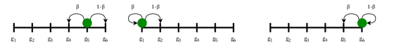
Figure 1: When $k=6$, three examples showing how the parameter value of a $\mathsf{GTFT}$ node is probabilistically updated under the $k$-IGT dynamics. Note that conditioned on a $\mathsf{GTFT}$ node $u$ being sampled as the first node, $u$ increments its parameter value with probability $(1-\beta)$ and decrements its parameter value with probability $\beta$ (where in both cases, the values are truncated to the range $[0,{\widehat{g}}]$).

Figure 1 shows an example of how the parameter value of a $\mathsf{GTFT}$ node is updated depending on the strategy type of its interaction partner.

Our results

Our main result characterizes the stationary and mixing properties of the $k$-IGT dynamics defined above. For an $(\alpha,\beta)$ population and any $k\geq 2$, we obtain the following:

Result 1 (see Theorem 2.4): The stationary distribution of the sequence $\{{\bf\it z}^{t}\}$ induced by the $k$-IGT dynamics is multinomial with parameters $m$ and $(p_{1},\dots,p_{k})$, where each $p_{j}\propto(1/\beta-1)^{j-1}$. Moreover, for $\beta\neq 1/2$, the mixing time of the dynamics is bounded by $O(kn\log n)$ total interactions, and when $\beta=1/2$, the dependence on $k$ changes to $k^{2}$.

Intuitively, this shows that after roughly $O(kn\log n)$ total interactions (for $\beta\neq 1/2$), the $k$-IGT dynamics induces a non-trivial distribution over $\mathsf{GTFT}$ strategies, with interesting dependencies on $\beta$ and $k$: for $\beta$ decreasing and $k$ increasing, we expect the average generosity parameter to be increasingly concentrated toward ${\widehat{g}}$, the maximum possible setting. We obtain this result by reducing the evolution of the $k$-IGT dynamics to a family of high-dimensional, weighted Ehrenfest random walks, which generalize the classic two-dimensional Ehrenfest urn process [ehrenfest1907zwei]. The stationary and mixing results we prove for these new Ehrenfest processes may be of independent interest.

In addition, we characterize the optimality of the $k$-IGT dynamics in the following mean-field regime: we consider the expected payoff of a $\mathsf{GTFT}$ node playing against a randomly chosen opponent from the $(\alpha,\beta)$ population, and assuming that all $\mathsf{GTFT}$ nodes play using an average parameter $g$. Then for the average generosity parameter value ${\widetilde{g}}_{k}$ under the stationary distribution of the $k$-IGT dynamics, and for the class of donation game payoff matrices, we show the following optimality gap:

Result 2 (see Theorem 2.7): Letting $g^{\star}$ denote the generosity parameter that maximizes the expected $\mathsf{GTFT}$ payoff in the mean-field regime, then $|g^{\star}-{\widetilde{g}}_{k}|\leq O(1/k)$ when the ratio $\beta/(1-\alpha-\beta)$ is bounded above by a small constant fraction.

This again highlights an interesting tradeoff between the size of the $\mathsf{GTFT}$ parameter space $k$, and on the optimality of the average generosity under the stationary distribution of the dynamics. The formal statement in Theorem 2.7 more precisely characterizes the constraint on $\beta/(1-\alpha-\beta)$ needed for the convergence to hold, and an interesting open question is to determine whether there exists a family of dynamics that converges to optimal under all regimes of this ratio.

1.4 Related work

Population protocol dynamics

The population model was originally introduced by Angluin et al. [DBLP:journals/dc/AngluinADFP06] to model computation in populations of passively mobile agents (such as sensor networks or animal populations), and has since found several other applications, from chemical reaction networks [Doty14, LCK16, CCDS15] to computing via synthetic DNA strands [CDSPCSS13]. On the theoretical side, an impressive amount of effort has been invested in understanding the computational power of the model, e.g. [DBLP:journals/dc/AngluinADFP06, AAE08], on analyzing fundamental dynamics such as rumor spreading and averaging [giakkoupis2016asynchrony, becchetti2018average], and on the complexity of core algorithmic tasks such as majority (consensus) [DV12, PVV09, becchetti2014plurality, alistarh2015fast, Berenbrink16, GP16, AAG18, becchetti2020consensus, doty2022time] and leader election [fischer2006self, AG15, DS18, GS18, berenbrink2020optimal] in this model. The latter direction has recently lead to tight bounds on the space and task complexity of these tasks [AAG18, berenbrink2020optimal, doty2022time]. In this context, our contributions are to design and analyze a novel class of repeated game dynamics that lead to interesting time and space tradeoffs.

Evolutionary game dynamics

There is a huge literature on evolutionary game dynamics. We briefly mention some key results and the relationship to our work. The first approach is to consider evolutionary dynamics in an infinite population with the aid of differential equations (aka, the replicator dynamics) [smith1982evolution, nowak2006evolutionary], and the goal is to study the existence and stability of equilibrium points. The second approach is to consider evolutionary dynamics in a finite population with a class of strategies e.g., reactive strategies or memory-1 strategies. In these approaches, the class of strategies is uncountable and simulation results suggest which strategies successfully evolve in the simulation of evolutionary dynamics [nowak1992tit, nowak1993strategy]. The third approach is to consider evolutionary dynamics on networks but with only two strategy types ($\mathsf{ALLC}$ and $\mathsf{ALLD}$) [lieberman2005evolutionary, allen2017evolutionary]. In contrast to the present paper, none of these works focus on quantitative aspects related to the mixing time (or convergence time) to the stationary behavior.

Other multi-player game settings

There is a large body of literature on a multi-player game setting [cesa2006prediction, nisan2007algorithmic], in which $n$ players simultaneously choose actions at each round, and receive a payoff according to a reward function that depends on the actions of all other players. In this setting, extensive work has been devoted to designing local strategies that provably converge to equilibria (over the space of all simultaneous player actions), and to determine their corresponding rates of convergence (e.g., [cai2011minmax, lin2020finite, golowich2020tight]). This is in contrast to the setting of the present work, where only a single random pair of nodes interacts at each round, and thus the results are not directly comparable. An orthogonal line of work to ours previously investigated game theoretic aspects of population protocols [bournez2009playing, bournez2013population], but the focus in these works is on understanding the computational power of interaction rules that correspond to symmetric games.

2 Technical overview of results

2.1 Preliminaries

Notation

We use the shorthand notation $[k]=\{1,\dots,k\}$ for any $k\geq 0$, and we define the set $\Delta^{m}_{k}:=\big{\{}(x_{1},\dots,x_{k})\in\mathbb{N}^{k}\;:\;\sum_{j\in[k]}x_{j}=m\big{\}}$. For non-negative integers $x$, $a$, and $b$, we write $[x]_{a}^{b}$ to denote $x$ truncated to the range $[a,b]$. For readability, when $a$ and $b$ are clear from context, we will (by slight abuse of notation) simply write $[x]$.

Markov chains

We consider discrete-time Markov chains $\{{{\bf\it x}}^{t}\}$ over a discrete space $\Omega$, with transition matrix ${\bf\it P}:\Omega\times\Omega\to[0,1]$. Recall that $\boldsymbol{\pi}:\Omega\to[0,1]$ is a stationary distribution of $\{{{\bf\it x}}^{t}\}$ if $\boldsymbol{\pi}{\bf\it P}=\boldsymbol{\pi}$ (where we interpret the probability mass function (PMF) of $\boldsymbol{\pi}$ as row vector). Recall also that any distribution ${\bf\it\nu}:\Omega\to[0,1]$ satisfying the detailed balance equations ${\bf\it\nu}({{\bf\it x}}){\bf\it P}({{\bf\it x}},{\bf\it y})={\bf\it\nu}({\bf\it y}){\bf\it P}({\bf\it y},{{\bf\it x}})$ for all ${{\bf\it x}},{\bf\it y}\in\Omega$ is a stationary distribution for the process. Starting from ${{\bf\it x}}^{1}:={{\bf\it x}}$ for any ${{\bf\it x}}\in\Omega$, we let ${\bf\it P}^{t}({{\bf\it x}})$ denote the the distribution of ${{\bf\it x}}^{t}$ (i.e., of the process after $t$ steps), and we write $d(t):=\max_{{{\bf\it x}}\in\Omega}\|{\bf\it P}^{t}({{\bf\it x}})-\boldsymbol{\pi}\|_{\text{TV}}$ to denote the distance to stationarity (in total variation) of the process after $t$ steps, maximized over all initial states. Then we define the mixing time $t_{\text{mix}}$ of $\{{{\bf\it x}}^{t}\}$ as $t_{\text{mix}}:=\min\{t\geq 0\;:\;d(t)\leq 1/4\}$. We refer the reader to the text of Levin and Peres [levin2017markov] for more background and preliminaries on Markov chains and mixing times.

Multinomial distributions

We recall basic facts about multinomial distributions. For $m\geq 1$, $k\geq 2$, and a sequence $(p_{1},\dots,p_{k})$ such that $p_{1}+\dots+p_{k}=1$, a distribution ${\bf\it\nu}$ is multinomial with parameters $m$ and $(p_{1},\dots p_{k})$ if the PMF of ${\bf\it\nu}$ is given by ${\bf\it\nu}({{\bf\it x}})\;=\;p_{1}^{x_{1}}\cdot p_{2}^{x_{2}}\dots p_{k}^{x_{k}}\cdot\binom{m}{x_{1},\dots,x_{k}}$ for all ${{\bf\it x}}=(x_{1},\dots,x_{k})\in\Delta^{m}_{k}$, where the multinomial coefficient is defined as $\binom{m}{x_{1},\dots,x_{k}}\;=\;\frac{m!}{x_{1}!\cdot x_{2}!\dots x_{k}!}$ . Writing ${\bf\it\nu}=(\nu_{1},\dots,\nu_{k})$, it is known that $\mathbb{E}[\nu_{j}]=m\cdot p_{j}$ for all $j\in[k]$. When $k=2$, then ${\bf\it\nu}$ is a binomial distribution, and we can simply say that ${\bf\it\nu}$ is binomial with parameters $m$ and $p_{1}$.

2.2 Stationary and mixing properties of $k$-IGT dynamics

2.2.1 Analysis setup

Our main result (Theorem 2.4) characterizes the stationary and mixing properties of the distribution of $\mathsf{GTFT}$ strategies under the $k$-IGT dynamics. For this, let $m:=n\cdot(1-\alpha-\beta)$ denote the number of $\mathsf{GTFT}$ nodes in the population, and fix $k\geq 2$. Recall we define ${\bf\it z}^{t}:=(z^{t}_{1},\dots,z^{t}_{k})\in\Delta^{m}_{k}$ as the count vector specifying the number of nodes with strategy $\mathsf{GTFT}(g_{i})$ after the $t$’th step, and we study the Markov chain $\{{\bf\it z}^{t}\}$. For this, we begin by specifying how the transitions of the $k$-IGT dynamics map to the transitions ${\bf\it z}^{t}\to{\bf\it z}^{t+1}$: recall from Definition 1.1 that following any (non-null) interaction, exactly one $\mathsf{GTFT}$ node updates its parameter. Then conditioned on an interaction at step $t$ whose initiator has strategy $\mathsf{GTFT}(g_{j})$ for some $j\in[k]$, then the coordinates of ${\bf\it z}^{t+1}$ can be specified by one of the following cases, depending on the strategy of the sampled interaction partner:

1. If the second player has strategy $\mathsf{ALLC}$ or $\mathsf{GTFT}$, then for each $j\in[k]$:

   $$z^{t+1}_{i}=\begin{aligned} \begin{cases}\;z^{t}_{i}-1&\text{if $i=j$ and $j<k$}\\ \;z^{t}_{i}+1&\text{if $i=j+1$ and $j<k$}\\ \;z^{t}_{i}&\text{otherwise.}\end{cases}\end{aligned}$$

2. If the second player has strategy $\mathsf{ALLD}$, then for each coordinate $i\in[k]$:

   $$z^{t+1}_{i}=\begin{aligned} \begin{cases}\;z^{t}_{i}-1&\text{if $i=j$ and $j>1$}\\ \;z^{t}_{i}+1&\text{if $i=j-1$ and $j>1$}\\ \;z^{t}_{i}&\text{otherwise.}\end{cases}\end{aligned}$$

Given that the pair of interacting nodes are sampled uniformly at random at each time step, this implies that the update in (a) occurs with (unconditional) probability $(z^{t}_{j}/n)\cdot(1-\beta)$, and the update in (b) occurs with probability $(z^{t}_{j}/n)\cdot\beta$. Then given ${\bf\it z}^{t}$, we can summarize all transitions ${\bf\it z}^{t}\to{\bf\it z}^{t+1}$ (for ${\bf\it z}^{t+1}\neq{\bf\it z}^{t}$) that occur with non-zero probability as follows: for all $j\in[k-1]$,

$${\bf\it z}^{t+1} \;=\;(z^{t}_{1},\dots,z^{t}_{j}-1,z^{t}_{j+1}+1,\dots,z^{t}_{k})\;\;\;\text{w.p. $\tfrac{z^{t}_{j}}{m}\cdot(1-\alpha-\beta)(1-\beta)$}$$ (1)

$$\text{and}\;\;\;{\bf\it z}^{t+1} \;=\;(z^{t}_{1},\dots,z^{t}_{j}+1,z^{t}_{j+1}-1,\dots,z^{t}_{k})\;\;\;\text{w.p. $\tfrac{z^{t}_{j+1}}{m}\cdot(1-\alpha-\beta)\beta$}\;\;.$$

Observe that transition probabilities in (1) are normalized by $m$ (using the definition $n=m/(1-\alpha-\beta)$), and that the coefficients $(1-\alpha-\beta)(1-\beta)$ and $(1-\alpha-\beta)(\beta)$ are absolute constants with respect to the coordinates of ${\bf\it z}^{t}$. Thus we can view the process as a special case of a more general class of Markov chains $\{{{\bf\it x}}^{t}\}$ over $\Delta^{m}_{k}$, whose transition probabilities (up to the absolute constant coefficients) are of the form in expression (1). We proceed to define and analyze this more general set of processes, from which characterizing the stationary and mixing properties of $\{{\bf\it z}^{t}\}$ will follow.

2.2.2 High-dimensional, weighted Ehrenfest processes

We introduce and analyze a more general class of random walks on $\Delta^{m}_{k}$, which we refer to as high-dimensional, weighted Ehrenfest processes. Defined formally:

Definition 2.1 ($(k,a,b,m)$-Ehrenfest Process).

Fix $k\geq 2$, and $a,b>0$ such that $a+b\leq 1$. Let $\{{{\bf\it x}}^{t}\}$ be the Markov chain on $\Delta^{m}_{k}$ with transition matrix ${\bf\it P}:\Delta^{m}_{k}\to\Delta^{m}_{k}$, where for all $j\in[k-1]$ and ${{\bf\it x}}=(x_{1},\dots,x_{k})\in\Delta^{m}_{k}$:

$${\bf\it P}\big{(}{{\bf\it x}},(x_{1},\dots,x_{j}-1,x_{j+1}+1,\dots,x_{k})\big{)}\;=\;p^{j,j+1}_{{\bf\it x}}\;:=\;a\cdot\frac{x_{j}}{m}$$

$${\bf\it P}\big{(}{{\bf\it x}},(x_{1},\dots,x_{j}+1,x_{j+1}-1,\dots,x_{k})\big{)}\;=\;p^{j+1,j}_{{\bf\it x}}\;:=\;b\cdot\frac{x_{j+1}}{m}$$

$${\bf\it P}({{\bf\it x}},{{\bf\it x}})\;=\;p^{\bot}_{{\bf\it x}}\;:=\;1-\Big{(}{\textstyle\sum_{j=1}^{k-1}}\;p^{j,j+1}_{{\bf\it x}}+p^{j+1,j}_{{\bf\it x}}\Big{)}\;,$$

and ${\bf\it P}({{\bf\it x}},{\bf\it y})=0$ for all other ${\bf\it y}\in\Delta^{m}_{k}$. Then we call $\{{{\bf\it x}}^{t}\}$ the $(k,a,b,m)$-Ehrenfest process.

Relationship to the two-urn Ehrenfest Process

When $k=2$ and $a=b=\frac{1}{2}$, the process reduces to the classical Ehrenfest Urn Process [ehrenfest1907zwei, takacs1979urn, grimmett2020probability] from statistical physics. Here, $m$ balls are distributed in two urns. At each step, an urn is sampled proportionally to its load, and with probability half, a ball from the sampled urn is placed into the other urn. The $(k,a,b,m)$-Ehrenfest process generalizes this original setting to a weighted, high-dimensional regime: we consider $m$ balls distributed over a sequence of $k$ urns, and after sampling the $j$’th urn proportionally to its load, a ball from urn $j$ is placed into urn $[j+1]$ with probability $a$, and into urn $[j-1]$ with probability $b$. While the stationary and mixing behavior of two-urn process (including several weighted variants) is well-studied [kac1947random, karlin1965ehrenfest, krafft1993mean, dette1994generalization, diaconis2011mathematics, mitzenmacher2017probability], we give the first such analyses for the weighted, high-dimensional analogs from Definition 2.1.

Deriving the stationary distributions

We exactly characterize the stationary distributions of $(k,a,b,m)$-Ehrenfest processes: we show these distibutions are multinomial with parameters $(p_{1},\dots,p_{k})$, and $m$, where each $p_{j}\propto(a/b)^{j-1}$. For $k=2$ and 3, this is obtained by viewing the process as a weighted random walk on a graph with vertex set $\Delta^{m}_{k}$, and by solving the recurrences stemming from the detailed balance equations (these calculations are derived formally in Sections 4.1 and 4.2). For higher dimensions (i.e., general $k$), we use the form of the stationary PMFs for $k=2$ and 3 as an Ansatz for the specifying and verifying (via the detailed balance equations) the stationary PMF. Stated formally, we prove the following result, the proof of which is given in Section 4.3.

Theorem 2.2.

Fix $a,b>0$ with $a+b\leq 1$, and let $\lambda:=a/b$. For any $k,m\geq 2$, let $\{{{\bf\it x}}^{t}\}$ be the $(k,a,b,m)$-Ehrenfest process, and let $\boldsymbol{\pi}:\Delta^{m}_{k}\to[0,1]$ be its stationary distribution. Then $\boldsymbol{\pi}$ is multinomial with parameters $m$ and $(p_{1},\dots,p_{k})$, where $p_{j}:=\frac{\lambda^{(j-1)\cdot x_{j}}}{\sum_{i=1}^{k}\lambda^{i-1}}$ for all $j\in[k]$.

Bounds on mixing times

Let $t_{\text{mix}}$ and $d(t)$ denote the mixing time and distance to stationarity (as defined in Section 2.1) of the $(k,a,b,m)$-Ehrenfest process. To derive bounds on $t_{\text{mix}}$, we introduce the following coupling: first, let $\{X_{t}\}$ and $\{Y_{t}\}$ be random walks over $\Omega=\{1,\dots,k\}^{m}$. At time $t$, we sample a coordinate $i\in[m]$ uniformly at random, and simultaneously increment or decrement the $i$’th coordinate of both $X_{t}$ and $Y_{t}$ (with values truncated to $[k]$) with probability $a$ and $b$, respectively.

It is straightforward to see that the vector of counts of each value $j\in[k]$ in both $X_{t}$ and $Y_{t}$ evolve as $(k,a,b,m)$-Ehrenfest processes. Then using the standard relationship between the coupling time of $\{(X_{t},Y_{t})\}$ (i.e., the first time $t$ when $X_{t}=Y_{t}$) and mixing times [levin2017markov], it suffices to probabilistically bound the coupling time of the joint process to derive the following bound on $t_{\text{mix}}$:

Theorem 2.3.

Fix $a,b>0$ with $a+b\leq 1$, and $k,m\geq 2$. Let $t_{\text{mix}}$ be the mixing time of the $(k,a,b,m)$-Ehrenfest process. Then

$$t_{\text{mix}}\;=\;\begin{aligned} \begin{cases}\;O\big{(}\min\{\frac{k}{|a-b|},k^{2}\}\cdot m\log m\big{)}\;\;\;&\text{when $a\neq b$}\\ \;O\big{(}k^{2}\cdot m\log m\big{)}\;\;\;&\text{when $a=b$}\end{cases}\end{aligned}\;\;.$$

We bound the coupling time of $(X_{t},Y_{t})$ by estimating the time to coalesce each of the $m$ coordinates of the process, and this reduces to bounding the expected absorption times of $m$ independent (possibly) biased random walks on $\{-k,\dots,k\}$ (which necessitates the case distinction between $a\neq b$ and $a=b$). The full coupling details and proof of the theorem are developed in Section 4.4, which requires a more careful coupling analysis compared to the original two-urn process.

Note also that $O(m\log m)$ is a known lower bound on the mixing time of the original two-urn process [diaconis1990asymptotic, levin2017markov], which means the dependence on $m$ in Theorem 2.3 is also tight in general. We suspect the linear dependence on $k$ is also optimal, but we leave obtaining such a lower bound as an open problem. Note also that the original two-urn process is known to exhibit a cut-off phenomenon [basu2014characterization], in which the distance to stationarity of the process sharply decays precisely at around $\frac{1}{2}\cdot n\log n$ steps  [levin2017markov]. Investigating this phenomenon for the general $(k,a,b,m)$ process (and obtaining such exact cutoff constants in terms of $a$ and $b$) is an interesting line of future work.

2.2.3 Combining the pieces

By combining the arguments of Sections 2.2.1 and 2.2.2, we can reduce the analysis of the $k$-IGT dynamics to that of a $k$-dimensional, weighted Ehrenfest process and formally state our main results. Specifically, based on the transition probabilities in (1), for any $k\geq 2$, the sequence $\{{\bf\it z}_{t}\}$ induced by the $k$-IGT dynamics is a $(k,a,b,m)$-Ehrenfest process, where $a:=(1-\alpha-\beta)(1-\beta)$, $b:=(1-\alpha-\beta)\beta$, and $m=(1-\alpha-\beta)n$. Then as a direct consequence of Theorems 2.2 and 2.3, we have the following main result characterizing the stationary and convergence behavior of the $k$-IGT dynamics:

Theorem 2.4.

Fix $k\geq 2$, and consider the vectors $\{{\bf\it z}^{t}\}$ induced by the $k$-IGT dynamics on an $(\alpha,\beta)$ population and an $RPD$ game setting with maximum generosity parameter $\widehat{g}$. Then $\{{\bf\it z}^{t}\}$ converges to a multinomial stationary distribution $\boldsymbol{\pi}$ with parameters $m$ and $(p_{1},\dots,p_{k})$, where $p_{j}=\frac{(1/\beta-1)^{(j-1)}}{\sum_{i=1}^{k}(1/\beta-1)^{(i-1)}}$ for each $j\in[k]$. Moreover the mixing time of $\{{\bf\it z}^{t}\}$ is bounded by $O\big{(}\min\{\frac{k}{|1-2\beta|},k^{2}\}\cdot n\log n\big{)}$ when $\beta\neq\frac{1}{2}$, and by $O\big{(}k^{2}\cdot n\log n\big{)}$ when $\beta=\frac{1}{2}$.

Observe that the mixing time of the process speeds up in regimes where $\beta$ is bounded away from half (i.e., the number of $\mathsf{ALLD}$ nodes is sufficiently small or sufficiently large). Similarly, the mean of the stationary distribution $\mathbb{E}[\boldsymbol{\pi}]=(\mathbb{E}[\pi_{1}],\dots,\mathbb{E}[\pi_{k}])$ grows increasingly less uniform over $[k]$ in this regime of $\beta$. In particular, given that $\boldsymbol{\pi}$ is a multinomial distribution, it follows that $\mathbb{E}[\pi_{j}]=m\cdot p_{j}$ for each $j\in[k]$. Thus for $\beta<1/2$, we expect the largest generosity parameter $g_{k}\in\mathcal{G}$ to have the greatest adoption among $\mathsf{GTFT}$ nodes after $t_{\text{mix}}$ many steps, and this mass increases as $\beta$ grows smaller, and as the size of the parameter space $k$ increases.

Average stationarity generosity

Given the set of generosity values $\mathcal{G}^{k}=\{g_{1},\dots,g_{k}\}$ and any ${\bf\it z}=(z_{1},\dots,z_{k})\in\Delta^{m}_{k}$, we define the average generosity value specified by ${\bf\it z}$ as $\frac{1}{m}\sum_{j\in[k]}g_{j}\cdot z_{j}$. Then the stationary distribution $\boldsymbol{\pi}$ from Theorem 2.4 allows us to derive an average stationary generosity value ${\widetilde{g}}_{k}$ for the $k$-IGT dynamics, which we define as the average generosity value with respect to $\widetilde{{\bf\it z}}:=\mathbb{E}[\boldsymbol{\pi}]$. We derive this value for all $k\geq 2$ in the following proposition:

Proposition 2.5.

Fix $k\geq 2$, and let $\boldsymbol{\pi}=(\pi_{1},\dots,\pi_{k})$ denote the stationary distribution of the $k$-IGT dynamics from Theorem 2.4 on an $(\alpha,\beta)$ population with maximum generosity parameter ${\widehat{g}}$. Let $\mathcal{G}^{k}$ be the set of parameter values from Definition 1.1. Define $\widetilde{g}_{k}:=(1/m)\sum_{j\in[k]}g_{j}\cdot\mathbb{E}[\pi_{j}]$ as the average stationary generosity of the dynamics, and let $\lambda:=(1-\beta)/\beta$. Then ${\widetilde{g}}_{k}={\widehat{g}}/2$ for $\beta=1/2$, and ${\widetilde{g}}_{k}={\widehat{g}}\cdot\Big{(}\frac{\lambda^{k}}{\lambda^{k}-1}-\big{(}\frac{1}{k-1}\big{)}\big{(}\frac{\lambda}{\lambda-1}\big{)}\big{(}\frac{\lambda^{k-1}-1}{\lambda^{k}-1}\big{)}\Big{)}$ for $\beta\neq 1/2$.

Roughly speaking, Proposition 2.5 shows that ${\widetilde{g}}_{k}\approx{\widehat{g}}\cdot\big{(}1-\frac{\beta}{(1-2\beta)k}\big{)}$ when $\beta$ is bounded below $1/2$, and ${\widetilde{g}}_{k}\approx{\widehat{g}}\cdot\big{(}\frac{1-\beta}{(2\beta-1)k}\big{)}$ when $\beta$ is bounded above $1/2$. Thus when the fraction of $\mathsf{ALLD}$ nodes is sufficiently small, the average stationary generosity approaches the maximum generosity parameter $\widehat{g}$ at a rate of $O(1/k)$, and it approaches $0$ at this same rate otherwise. This again highlights the tradeoffs between the size of the parameter space $k$, and the resulting levels of generosity induced by the dynamics. The proof of the proposition is given in Section 5.

2.3 Characterizing the optimality of $k$-IGT dynamics

2.3.1 Expected payoffs in repeated PD games

We characterize several game-theoretic properties of the $k$-IGT dynamics. First, for a pair of strategies $\mathsf{S}_{1},\mathsf{S}_{2}\in\mathcal{S}:=\{\mathsf{ALLC},\mathsf{ALLD},\mathsf{GTFT}\}$, let $f\big{(}\mathsf{S}_{1};\mathsf{S}_{2}\big{)}$ denote the expected payoff in an RPD game (over the randomness of the strategies and repeated rounds) for a node with strategy $\mathsf{S}_{1}$ against an opponent with strategy $\mathsf{S}_{2}$. In Section 6.1, we define $f$ more precisely, and we compute $f\big{(}\mathsf{GTFT}(g);\mathsf{S}\big{)}$ for $\mathsf{GTFT}$ nodes against opponents with strategy $\mathsf{S}\in\mathcal{S}$. In particular, each $f\big{(}\mathsf{GTFT}(g);\mathsf{S}\big{)}$ requires specifying the Markov chain over the repeated game states (which changes with $\mathsf{S}$), and then tracking how the distribution over the $\mathsf{GTFT}$ node’s single-round payoffs evolves over rounds.

Bridging $k$-IGT and introspection dynamics

Under mild constraints on the reward vector ${\bf\it v}$ and maximum generosity parameter ${\widehat{g}}$, we show that the transition rules of the $k$-IGT dynamics are locally optimal in the following sense: under any transition rule of Definition 1.1, the expected payoff $f\big{(}\mathsf{GTFT}(g);\mathsf{S}\big{)}$ will never decrease had the $\mathsf{GTFT}$ node used the updated parameter value specified by the transition rules against its previous opponent with strategy $\mathsf{S}$. In particular, this bridges the relationship between the $k$-IGT dynamics and the classic concept of introspection dynamics with local search from evolutionary games [hofbauer1998evolutionary], where an individual explores the local neighborhood of its strategy space to adopt a new strategy that would have performed better. Formally, we prove:

Proposition 2.6.

Consider an RPD game setting consisting of (a) a reward vector ${\bf\it v}=[R,T,S,P]^{\top}$ with $R+P\leq T+S$, (b) a restart probability $\delta>\tfrac{T-R}{R-S}$, (c) a maximum generosity parameter $\widehat{g}<1-\frac{T-R}{\delta(R-S)}$, and (d) an initial $\mathsf{GTFT}$ cooperation probability $s_{1}\in[0,1)$. Then for all $g,g^{\prime}\in[0,\widehat{g}]$ such that $g<g^{\prime}$, the following three statements hold:

(i) $$f\big{(}\mathsf{GTFT}(g);\mathsf{GTFT}(g^{\prime\prime})\big{)}\;<\;f\big{(}\mathsf{GTFT}(g^{\prime});\mathsf{GTFT}(g^{\prime\prime})\big{)}\;\;\;\text{for all $g^{\prime\prime}\in[0,\widehat{g}]$}$$

(ii) $$f\big{(}\mathsf{GTFT}(g);\mathsf{ALLC}\big{)}\;\leq\;f\big{(}\mathsf{GTFT}(g^{\prime});\mathsf{ALLC}\big{)}$$

(iii) $$f\big{(}\mathsf{GTFT}(g);\mathsf{ALLD}\big{)}\;>\;f\big{(}\mathsf{GTFT}(g^{\prime});\mathsf{ALLD}\big{)}.$$

Note that statement (ii) of the proposition implies that only the expected payoff $f$ for nodes playing strategy $\mathsf{GTFT}(g)$ against $\mathsf{ALLC}$ is non-decreasing with $g$, whereas statements (i) and (iii) give strictly increasing inequalities with respect to $g$. We remark that the $k$-IGT transitions could thus be adjusted such that $\mathsf{GTFT}$ nodes only increase their parameter following an interaction with a second $\mathsf{GTFT}$ node: this would ensure strictly increasing expected payoff relationships for each transition type, but at the expense of lower average stationary generosity values (in the sense of Proposition 2.5, and depending on the ratio of $\mathsf{GTFT}$ to $\mathsf{ALLC}$ nodes). Observe also that condition (a) in the proposition is always satisfied by donation game reward vectors.

2.3.2 Optimality of the average stationary generosity in the mean-field setting

Using the formulations of the previous section, we consider the expectation of $f\big{(}\mathsf{GTFT};\mathsf{S}\big{)}$, when the opposing strategy $\mathsf{S}\in\mathcal{S}$ is drawn from an $(\alpha,\beta)$ population (and thus the randomness is over both the rounds of the RPD game, and the interaction sampling in the population). In particular, using the notion of the average generosity from Section 2.2.3, we consider a mean-field approximation (similar in spirit to, e.g., [lasry2007mean]), in which all $\mathsf{GTFT}$ nodes have the average generosity parameter value. For this, recall that $m=n(1-\alpha-\beta)$. We will write $f_{g}\big{(}\mathsf{S}\big{)}$ as shorthand for $f\big{(}\mathsf{GTFT}(g);\mathsf{S}\big{)}$, and for any average generosity value $g\in[0,\widehat{g}]$, we define

$$F\big{(}g,\alpha,\beta\big{)}\;:=\;\alpha\cdot f_{g}\big{(}\mathsf{ALLC}\big{)}+\beta\cdot f_{g}\big{(}\mathsf{ALLD}\big{)}+\tfrac{m}{n}\cdot f_{g}\big{(}\mathsf{GTFT}(g)\big{)}\;.$$ (2)

Here, $F(g,\alpha,\beta)$ exactly captures the expected RPD payoff of a $\mathsf{GTFT}$ node in an $(\alpha,\beta)$ population, and in this mean-field approximation with average generosity $g$: at its next interaction, a $\mathsf{GTFT}$ node with parameter $g$ plays against an $\mathsf{ALLC}$ or $\mathsf{ALLD}$ node with probability $\alpha$ or $\beta$, respectively, and against a second $\mathsf{GTFT}$ node with the average parameter $g$ with probability $m/n$.

Let $g^{\star}:=\operatorname{argmax}_{g\in[0,{\widehat{g}}]}F(g,\alpha,\beta)$ denote the average generosity value that maximizes this expected payoff. Then letting ${\widetilde{g}}_{k}$ denote the average stationary generosity value of the $k$-IGT dynamics from Propsition 2.5, we characterize the convergence of ${\widetilde{g}}_{k}\to g^{\star}$ with $k$ for the special class of donation game payoff matrices in the following theorem:

Theorem 2.7.

Consider an $(\alpha,\beta)$ population, and a donation game RPD setting with reward vector ${\bf\it v}=[b-c,-c,b,0]^{\top}$, a maximum generosity parameter ${\widehat{g}}$ satisfying Proposition 2.6, and an initial $\mathsf{GTFT}$ cooperation probability $s_{1}=1/2$. For any $k\geq 2$, let ${\widetilde{g}}_{k}$ denote the average stationary generosity value of the $k$-IGT dynamics as in Proposition 2.5. Define $g^{\star}:=\operatorname{argmax}_{g\in[0,{\widehat{g}}]}F(g,\alpha,\beta)$, and let $\phi:=\frac{\beta n}{m}$. Then for $\lambda:=\frac{1-\beta}{\beta}>1$ and $\phi\leq\frac{(b-c)(1-\delta)}{2c(1-\delta(1-{\widetilde{g}}))^{2}}$, we have $\big{|}g^{\star}-\widetilde{g}_{k}\big{|}\leq\frac{\beta}{(1-2\beta)(k-1)}$.

Roughly speaking, the theorem shows that when the ratio of $\mathsf{ALLD}$ nodes to $\mathsf{GTFT}$ nodes $\phi$ is sufficiently small, and assuming the $k$-IGT dynamics has converged to its stationary distribution, then the average generosity value ${\widetilde{g}}_{k}$ will be close to optimal (i.e., close to the maximizing parameter value $g^{\star}$), and that this gap vanishes at a rate of roughly $O(1/k)$. The proof of the theorem (developed in Section 6.2) first uses convexity arguments to characterize the maximizer of $F(g,\alpha,\beta)$ with respect to $\phi$, and then uses the average stationary generosity calculation from Proposition 2.5, which translates into a convergence rate between ${\widetilde{g}}_{k}$ and $\widehat{g}$. We note also that the same convergence rate holds for other constant settings of $s_{1}$, but under slightly different constants constraining $\phi$.

Remarks on the formulation of $F(g,\alpha,\beta)$

Note that in the formulation of the expected $\mathsf{GTFT}$ payoff $F(g,\alpha,\beta)$ from expression (2), our use of the term “mean-field” in specifying $F$ is done mainly in an informal sense. In the related (but distinct) setting of mean-field games [lasry2007mean, cousin2011mean, cardaliaguet2010notes], one approximates the global behavior of $n$ locally interacting nodes by assuming that an individual node plays against the averaged behavior of the population, i.e., by assuming the opponent is a representative node drawn from some approximate, global distribution over strategies.

Note that we could also imagine formulating an alternative version of such an expected payoff by considering the more granular distribution of $\mathsf{GTFT}$ nodes over the parameters $\mathcal{G}^{k}$ that is specified by the stationary distribution $\boldsymbol{\pi}$ of the $k$-IGT dynamics. However, the resulting calculation expressing this expected payoff is difficult to control analytically, which arises from the complex nature of the function $f(\mathsf{S}_{1},\mathsf{S}_{2})$ when both $\mathsf{S}_{1}$, $\mathsf{S}_{2}$ are $\mathsf{GTFT}$ strategies with non-equal parameters. Nevertheless, we provide several numerical simulations in Section 6.3 suggesting that the values of $F$ using the mean-field assumptions are similar to the corresponding values of the more granular computation, even for small $m$.

3 Discussion

In this work, we introduced a family of dynamics for repeated prisoner’s dilemma games in the population protocol model, and we characterized their stationary and mixing properties by analyzing a new class of high-dimensional Ehrenfest processes. Our work opens the door for several future directions: first at a broad level, it would be interesting to study dynamics in this setting for other common repeated games from evolutionary dynamics, such as stag hunt and hawk dove [nowak2006evolutionary], and to investigate the resulting time-space tradeoffs. At a more technical level, it remains open to derive lower bounds that establish the optimal dependence on $k$ in the mixing times of the $(k,a,b,m)$-Ehrenfest process. Moreover, studying the cutoff behavior of these processes (and establishing the exact cutoff constants in terms of $k,a,b$) is left as open.

In the following sections, we provide more technical details on our results.

4 Details on high-dimensional, weighted Ehrenfest processes

In this section, we provide more details on the $(k,a,b,m)$-Ehrenfest processes introduced in Section 2.2.2. In particular, in Sections 4.1 and Sections 4.2 we derive the stationary distributions for the process when $k=2$ and $k=3$, respectively. We use the form of the PMFs of these distributions to derive expressions for the PMFs for larger (general) $k$, and we verify their stationarity in the proof of Theorem 2.2 in Section 4.3. In Section 4.4, we develop the proof of Theorem 2.3, which gives a bound on the mixing time of the process, which is based on the coupling introduced in Section 2.2.2.

For convenience, we restate the definition of the process here:

See 2.1

4.1 Deriving the stationary distribution for $k=2$

In this section we derive the PMF of the stationary distribution of the $(2,a,b,m)$-Ehrenfest process, for which we use the following, more convenient notation:

Setup and notation

Let $\{{{\bf\it x}}^{t}\}$ denote the process, and recall each ${{\bf\it x}}^{t}\in\Delta^{m}_{k}$. Let $\boldsymbol{\pi}:\Delta^{m}_{2}\to[0,1]$ denote its stationary distribution. Based on the transitions from Definition 2.1, it is easy to see that $\{{{\bf\it x}}^{t}\}$ is irreducible and aperiodic, and thus $\boldsymbol{\pi}$ is the unique stationary distribution of the process.

In order to specify the PMF of $\boldsymbol{\pi}$, we restrict our view of the process $\{x^{t}\}$ to its first coordinate $i\in\mathcal{Z}:=\{0,1,\dots,m\}$. In particular, we define the function $\pi:\mathcal{Z}\to[0,1]$ such that $\pi(i)=\boldsymbol{\pi}((i,m-i))$ for all $i\in\mathcal{Z}$. In other words, we project the set $\Delta^{m}_{2}$ onto the line $\mathcal{Z}=\{0,\dots,m\}$. We can then define the transition matix $P:\mathcal{Z}\times\mathcal{Z}\to[0,1]$ over pairs of points in $\mathcal{Z}$ that is induced by the matrix ${\bf\it P}$ for the process $\{{{\bf\it x}}^{t}\}$. Thus for any $x,y\in\mathcal{Z}$, the entries of $P$ are given by:

$$P\big{(}x,y\big{)}\;=\;\begin{aligned} \begin{cases}\;\text{if }y=[x+1]:&b\tfrac{m-x}{m}\\ \;\text{if }y=[x-1]:&a\tfrac{x}{m}\\ \;\text{if }y=x:&1-b+(b-a)\tfrac{x}{m}\\ \;\text{otherwise}:&0\end{cases}\end{aligned}\;\;.$$ (3)

Thus matrix $P$ specifies the transition probabilities over the number line $\mathcal{Z}$ for the first coordinate of the process $\{{{\bf\it x}}^{t}\}$ (and this entirely specifies the process given that each ${{\bf\it x}}^{t}\in\Delta^{m}_{2}$).

Then in the following proposition, we derive the PMF of $\pi$ by solving the system of equations arising from the detailed balance equations. The PMF of $\boldsymbol{\pi}$ is then recovered immediately based on the one-to-one relationship between $\pi$ and $\boldsymbol{\pi}$.

Proposition 4.1.

Fix $a,b>0$ with $a+b\leq 1$. Let $P:\mathcal{Z}\times\mathcal{Z}\to[0,1]$ denote the transition matrix induced by the $(2,a,b,m)$-Ehrenfest process (as defined in expression (3)) and let $\pi:\mathcal{Z}\to[0,1]$ be the stationary distribution of $P$. Letting $\lambda:=a/b$, we have for all $i\in\mathcal{Z}$:

$$\pi(i)\;=\;\frac{\lambda^{m-i}}{(1+\lambda)^{m}}\cdot\binom{m}{i}\;.$$

Proof.

We solve for the $\pi$ based on the system of equations stemming from the detailed balance equations

$$\pi(x)\cdot P(x,y)\;=\;\pi(y)\cdot P(y,x)\;,$$

which must hold for all $x,y\in\mathcal{Z}$. Then for any $i\in\mathcal{Z}$, we can recursively substitute the equations along the path $i,i-1,\dots,1,0$ to find

$$\pi(i)\;=\;\pi(0)\cdot\frac{P(0,1)\cdot P(1,2)\cdots P(i-1,i)}{P(i,i-1)\cdot P(i-1,i-2)\cdots P(1,0)}\;.$$

It then follows from the entries of $P$ defined in expression (3) that we can write

$$\pi(i)\;=\;\pi(0)\cdot\frac{bm\cdot b(m-1)\cdots b(m-i+1)}{ai\cdot a(i-1)\cdots a}\;=\;\pi(0)\cdot\Big{(}\frac{b}{a}\Big{)}^{i}\cdot\frac{m!}{(m-i)!\cdot i!}\;.$$ (4)

Given that $\sum_{i\in\mathcal{Z}}\pi(i)=1$ (as $\pi$ is a distribution), and recalling that $\lambda=a/b$, we then have

$$1\;=\;\sum_{i=0}^{m}\pi(0)\cdot\Big{(}\frac{1}{\lambda}\Big{)}^{i}\cdot\frac{m!}{(m-i)!\cdot i!}\;=\;\pi(0)\cdot\Big{(}1+\frac{1}{\lambda}\Big{)}^{m}\;=\;\pi(0)\cdot\Big{(}\frac{1+\lambda}{\lambda}\Big{)}^{m}\;,$$

where the second equality is due to the binomial theorem. It follows that $\pi(0)=\lambda^{m}/(1+\lambda)^{m}$, and substituting this into expression (4) for each $i\in\mathcal{Z}$ yields the statement of the proposition. ∎

Remark 4.2.

Given the relationship between $\pi$ and $\boldsymbol{\pi}$, it follows that for any ${{\bf\it x}}=(x_{1},x_{2})\in\Delta^{m}_{k}$:

$$\boldsymbol{\pi}({{\bf\it x}})\;=\;\frac{\lambda^{x_{2}}}{(1+\lambda)^{m}}\cdot\binom{m}{x_{1}}\;.$$

In other words, the stationary distribution of the $(2,a,b,m)$-Ehrenfest process is a binomial distribution with parameters $m$ and $p=1/(1+\lambda)$.

4.2 Deriving the stationary distribution for $k=3$

We now derive the stationary distribution for the $(3,a,b,m)$-Ehrenfest process. Our approach is similar in spirit to the $k=2$ case, but we require a more careful technique in order to solve for the stationary PMF in this higher-dimensional regime. For this, we begin by introducing a more convenient notation (similar to the notation used for the $k=2$ case).

Setup and notation

Let $\{{{\bf\it x}}^{t}\}$ denote the $(3,a,b,m)$-Ehrenfest process, and recall that its stationary distribution $\boldsymbol{\pi}$ is defined over the space $\Delta^{m}_{3}$. It is again easy to see that the Markov chain $\{{{\bf\it x}}^{t}\}$ is irreducible, and thus $\boldsymbol{\pi}$ is its unique stationary distribution. Similar to the $k=2$, when deriving the PMF for $\boldsymbol{\pi}$, it is more convenient to work over the (equivalent) set of points that are defined explicitly in a $(k-1)$-dimensional space.

$$\mathcal{X}\;:=\;\Big{\{}\Big{(}\genfrac{}{}{0.0pt}{1}{i}{j}\Big{)}\;:\;0\leq i,j\leq m\text{ and }i+j\leq m\Big{\}}\;,$$

where we use the one-to-one mapping $\Big{(}\genfrac{}{}{0.0pt}{1}{i}{j}\Big{)}\mapsto(i,j,m-i-j)\in\Delta^{m}_{3}$ for all $\Big{(}\genfrac{}{}{0.0pt}{1}{i}{j}\Big{)}\in\mathcal{X}$. Roughly speaking, we can view $\mathcal{X}$ as simply the set $\Delta^{m}_{3}$ embedded onto the two-dimensional plane.

Then we define $\pi:\mathcal{X}\to[0,1]$ as the PMF over $\mathcal{X}$ such that for all $(i,j,k)\in\Delta^{m}_{3}$, we have $\pi\Big{(}\genfrac{}{}{0.0pt}{1}{i}{j}\Big{)}=\boldsymbol{\pi}((i,j,k))$. Moreover, we let $P:\mathcal{X}\times\mathcal{X}\to[0,1]$ denote the probability transition function over pairs of points in $\mathcal{X}$ that is induced by the transition matrix ${\bf\it P}:\Delta^{m}_{3}\times\Delta^{m}_{3}\to[0,1]$ of the process $\{{{\bf\it x}}^{t}\}$. Then for any $(x_{1},x_{2}),(y_{1},y_{2})\in\mathcal{X}$, the entries of $P$ can be summarized as

$$P\Big{(}\Big{(}\genfrac{}{}{0.0pt}{1}{x_{1}}{x_{2}}\Big{)},\Big{(}\genfrac{}{}{0.0pt}{1}{y_{1}}{y_{2}}\Big{)}\Big{)}\;=\;\begin{aligned} \begin{cases}\;\text{if }\Big{(}\genfrac{}{}{0.0pt}{1}{y_{1}}{y_{2}}\Big{)}=\Big{(}\genfrac{}{}{0.0pt}{1}{[x_{1}-1]}{[x_{2}+1]}\Big{)}:&a\tfrac{x_{1}}{m}\vspace*{0.2em}\\ \;\text{if }\Big{(}\genfrac{}{}{0.0pt}{1}{y_{1}}{y_{2}}\Big{)}=\Big{(}\genfrac{}{}{0.0pt}{1}{[x_{1}+1]}{[x_{2}-1]}\Big{)}:&b\tfrac{x_{2}}{m}\vspace*{0.2em}\\ \;\text{if }\Big{(}\genfrac{}{}{0.0pt}{1}{y_{1}}{y_{2}}\Big{)}=\Big{(}\genfrac{}{}{0.0pt}{1}{x_{1}}{[x_{2}-1]}\Big{)}:&a\tfrac{x_{2}}{m}\vspace*{0.2em}\\ \;\text{if }\Big{(}\genfrac{}{}{0.0pt}{1}{y_{1}}{y_{2}}\Big{)}=\Big{(}\genfrac{}{}{0.0pt}{1}{x_{1}}{[x_{2}+1]}\Big{)}:&b\big{(}1-\tfrac{x_{1}+x_{2}}{m}\big{)}\vspace*{0.2em}\\ \;\text{if }\Big{(}\genfrac{}{}{0.0pt}{1}{y_{1}}{y_{2}}\Big{)}=\Big{(}\genfrac{}{}{0.0pt}{1}{x_{1}}{x_{2}}\Big{)}:&1-b\big{(}1-\tfrac{x_{1}}{m}\big{)}-a\tfrac{x_{1}+x_{2}}{m}\vspace*{0.2em}\\ \;\text{otherwise}:&0\end{cases}\end{aligned}\;\;\;\;.$$ (5)

For concreteness, Figure 2 shows an example of the space $\mathcal{X}$ and the transitions with non-zero probability under $P$ when $k=3$ and $m=3$. We then prove the following proposition specifying the PMF of $\pi$:

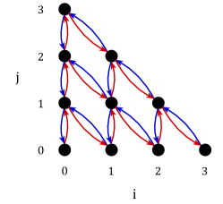
Figure 2: Example when $k=3$ and $m=3$ of the space $\mathcal{X}$ and the set of non-zero transitions specified by $P$ (denoted by a directed edge between two nodes). Transitions colored blue have coefficient $a$, and transitions colored red have coefficient $b$. Considering the outward transition edges from a node $\Big{(}\genfrac{}{}{0.0pt}{1}{i}{j}\Big{)}\in\mathcal{X}$, downward vertical transitions are weighted by $j/n$, upward vertical transitions are weighted by $(1-(i+j)/n)$, downward diagonal transitions are weighted by $j/n$, and upward diagonal transitions are weighted by $i/n$.

Proposition 4.3.

Fix $a,b>0$ with $a+b\leq 1$, let $P:\mathcal{X}\times\mathcal{X}\to[0,1]$ denote the transition matrix induced by the $(3,a,b,m)$-Ehrenfest process (as defined in expression (5)), and let $\pi:\mathcal{X}\to[0,1]$ be stationary distribution of $P$. Then letting $\lambda:=a/b$, we have

$$\pi\Big{(}\genfrac{}{}{0.0pt}{1}{i}{j}\Big{)}\;=\;\frac{\lambda^{2(m-i-j)}\lambda^{j}}{(1+\lambda+\lambda^{2})^{m}}\cdot\binom{m}{i,j,(m-i-j)}$$

for all $x=\Big{(}\genfrac{}{}{0.0pt}{1}{i}{j}\Big{)}\in\mathcal{X}$.

Proof.

It suffices to solve for $\pi$ from the system of equations arising from the detailed balance equations:

$$\pi\Big{(}\genfrac{}{}{0.0pt}{1}{x_{1}}{y_{1}}\Big{)}\cdot P\Big{(}{\Big{(}\genfrac{}{}{0.0pt}{1}{x_{1}}{y_{1}}\Big{)}},{\Big{(}\genfrac{}{}{0.0pt}{1}{x_{2}}{y_{2}}\Big{)}}\Big{)}\;=\;\pi\Big{(}\genfrac{}{}{0.0pt}{1}{x_{2}}{y_{2}}\Big{)}\cdot P\Big{(}{\Big{(}\genfrac{}{}{0.0pt}{1}{x_{2}}{y_{2}}\Big{)}},{\Big{(}\genfrac{}{}{0.0pt}{1}{x_{1}}{y_{1}}\Big{)}}\Big{)}\;,$$

which must hold for all pairs $(x_{1},y_{1}),(x_{2},y_{2})\in\mathcal{X}$. Using the recursive structure of the transition probabilities $P$ defined in expression (5), we can express each $\pi\Big{(}\genfrac{}{}{0.0pt}{1}{i}{j}\Big{)}$ in terms of $\pi\Big{(}\genfrac{}{}{0.0pt}{1}{0}{m}\Big{)}$ for all $\Big{(}\genfrac{}{}{0.0pt}{1}{i}{j}\Big{)}\in\mathcal{X}$ using the following formulations:

1. For any $j\in\{0,\dots,m\}$:

   $$\pi\Big{(}\genfrac{}{}{0.0pt}{1}{0}{j}\Big{)}\;=\;\pi\Big{(}\genfrac{}{}{0.0pt}{1}{0}{m}\Big{)}\cdot\frac{P\Big{(}{\Big{(}\genfrac{}{}{0.0pt}{1}{0}{m}\Big{)}},{\Big{(}\genfrac{}{}{0.0pt}{1}{0}{m-1}\Big{)}}\Big{)}\cdot P\Big{(}{\Big{(}\genfrac{}{}{0.0pt}{1}{0}{m-1}\Big{)}},{\Big{(}\genfrac{}{}{0.0pt}{1}{0}{m-2}\Big{)}}\Big{)}\cdots P\Big{(}{\Big{(}\genfrac{}{}{0.0pt}{1}{0}{j+1}\Big{)}},{\Big{(}\genfrac{}{}{0.0pt}{1}{0}{j}\Big{)}}\Big{)}}{P\Big{(}{\Big{(}\genfrac{}{}{0.0pt}{1}{0}{j}\Big{)}},{\Big{(}\genfrac{}{}{0.0pt}{1}{0}{j+1}\Big{)}}\Big{)}\cdot P\Big{(}{\Big{(}\genfrac{}{}{0.0pt}{1}{0}{j+1}\Big{)}},{\Big{(}\genfrac{}{}{0.0pt}{1}{0}{j+2}\Big{)}}\Big{)}\cdots P\Big{(}{\Big{(}\genfrac{}{}{0.0pt}{1}{0}{m-1}\Big{)}},{\Big{(}\genfrac{}{}{0.0pt}{1}{0}{m}\Big{)}}\Big{)}}\;\;.$$

2. For any $i\in\{1,\dots,m\}$ and $j\in\{0,\dots,m\}$:

   $$\pi\Big{(}\genfrac{}{}{0.0pt}{1}{i}{j}\Big{)}\;=\;\pi\Big{(}\genfrac{}{}{0.0pt}{1}{0}{j+i}\Big{)}\cdot\frac{P\Big{(}{\Big{(}\genfrac{}{}{0.0pt}{1}{0}{j+i}\Big{)}},{\Big{(}\genfrac{}{}{0.0pt}{1}{1}{j+i-1}\Big{)}}\Big{)}\cdot P\Big{(}{\Big{(}\genfrac{}{}{0.0pt}{1}{1}{j+i-1}\Big{)}},{\Big{(}\genfrac{}{}{0.0pt}{1}{2}{j+i-2}\Big{)}}\Big{)}\cdots P\Big{(}{\Big{(}\genfrac{}{}{0.0pt}{1}{i-1}{j+1}\Big{)}},{\Big{(}\genfrac{}{}{0.0pt}{1}{i}{j}\Big{)}}\Big{)}}{P\Big{(}{\Big{(}\genfrac{}{}{0.0pt}{1}{i}{j}\Big{)}},{\Big{(}\genfrac{}{}{0.0pt}{1}{i-1}{j+1}\Big{)}}\Big{)}\cdot P\Big{(}{\Big{(}\genfrac{}{}{0.0pt}{1}{i-1}{j+1}\Big{)}},{\Big{(}\genfrac{}{}{0.0pt}{1}{i-2}{j+2}\Big{)}}\Big{)}\cdots P\Big{(}{\Big{(}\genfrac{}{}{0.0pt}{1}{1}{j+1-i}\Big{)}},{\Big{(}\genfrac{}{}{0.0pt}{1}{0}{j+i}\Big{)}}\Big{)}}\;\;,$$

   from which it follows that $\pi\Big{(}\genfrac{}{}{0.0pt}{1}{i}{j}\Big{)}$ can be expressed in terms of $\pi\Big{(}\genfrac{}{}{0.0pt}{1}{0}{m}\Big{)}$ using the expression for $\pi\Big{(}\genfrac{}{}{0.0pt}{1}{0}{i+j}\Big{)}$ from (a).

Note that by viewing the transitions specified by $P$ as directed edges over the vertex set $\mathcal{X}$ (i.e., as in the example of Figure 2) the formulation in (a) follows by recursively substituting the expressions for $\pi\Big{(}\genfrac{}{}{0.0pt}{1}{0}{j}\Big{)}$ from the detailed balance equation along the path from $\Big{(}\genfrac{}{}{0.0pt}{1}{0}{j}\Big{)}$ to $\Big{(}\genfrac{}{}{0.0pt}{1}{0}{m}\Big{)}$ using only vertical edges. Similarly, the formulation in (b) follows by considering such paths from $\pi\Big{(}\genfrac{}{}{0.0pt}{1}{i}{j}\Big{)}$ to $\pi\Big{(}\genfrac{}{}{0.0pt}{1}{0}{i+j}\Big{)}$ using only diagonal edges. Then using the entries of $P$ defined in (5), we find for part (a) that, for any $j\in\{0,\dots,m\}$:

$$\pi\Big{(}\genfrac{}{}{0.0pt}{1}{0}{j}\Big{)}\;=\;\pi\Big{(}\genfrac{}{}{0.0pt}{1}{0}{m}\Big{)}\cdot\frac{am\cdot a(m-1)\cdots a(j+1)}{b(m-j)\cdot b(m-(j+1))\cdots b}\;=\;\pi\Big{(}\genfrac{}{}{0.0pt}{1}{0}{m}\Big{)}\cdot\Big{(}\frac{a}{b}\Big{)}^{m-j}\cdot\frac{m!}{j!\cdot(m-j)!}\;\;.$$ (6)

Similarly, for part (b), we find for any $i\in\{1,\dots,m\}$ and $j\in\{0,\dots,m\}$:

$$\pi\Big{(}\genfrac{}{}{0.0pt}{1}{i}{j}\Big{)}\;=\;\pi\Big{(}\genfrac{}{}{0.0pt}{1}{0}{j+i}\Big{)}\cdot\frac{b(j+i)\cdot b(j+i-1)\cdots b(j+1)}{ai\cdot a(i-1)\cdots a}\;=\;\pi\Big{(}\genfrac{}{}{0.0pt}{1}{0}{j+i}\Big{)}\cdot\Big{(}\frac{b}{a}\Big{)}^{i}\cdot\frac{(j+i)!}{j!\cdot i!}\;\;.$$ (7)

Then substituting the expression for $\pi\Big{(}\genfrac{}{}{0.0pt}{1}{0}{j+i}\Big{)}$ from (6), we can further simplify and write

$$\pi\Big{(}\genfrac{}{}{0.0pt}{1}{i}{j}\Big{)} \;=\;\pi\Big{(}\genfrac{}{}{0.0pt}{1}{0}{m}\Big{)}\cdot\Big{(}\frac{a}{b}\Big{)}^{m-(i+j)}\cdot\frac{m!}{(j+i)!\cdot(m-(i+j))!}\cdot\Big{(}\frac{b}{a}\Big{)}^{i}\cdot\frac{(j+i)!}{j!\cdot i!}$$

$$\;=\;\pi\Big{(}\genfrac{}{}{0.0pt}{1}{0}{m}\Big{)}\cdot\Big{(}\frac{a}{b}\Big{)}^{m-2i-j}\cdot\frac{m!}{(m-i-j)!\cdot i!\cdot j!}\;.$$ (8)

Now using the fact that $\pi$ is a distribution and thus $\sum_{x\in\mathcal{X}}\pi(x)=1$, and recalling that $\lambda=(a/b)$, we can use the expressions (6) and (8) to write:

$$1 \;=\;\pi\Big{(}\genfrac{}{}{0.0pt}{1}{0}{m}\Big{)}+\sum_{j=0}^{m-1}\bigg{(}\pi\Big{(}\genfrac{}{}{0.0pt}{1}{0}{j}\Big{)}+\sum_{i=1:\;i+j\leq m}^{m}\pi\Big{(}\genfrac{}{}{0.0pt}{1}{i}{j}\Big{)}\bigg{)}$$

$$\;=\;\pi\Big{(}\genfrac{}{}{0.0pt}{1}{0}{m}\Big{)}+\sum_{j=0}^{m-1}\bigg{(}\pi\Big{(}\genfrac{}{}{0.0pt}{1}{0}{m}\Big{)}\cdot\lambda^{m-j}\cdot\tfrac{m!}{j!\cdot(m-j)!}+\sum_{i=1:\;i+j\leq m}^{m}\;\pi\Big{(}\genfrac{}{}{0.0pt}{1}{0}{m}\Big{)}\cdot\lambda^{m-2i-j}\cdot\tfrac{m!}{(m-i-j)!\cdot i!\cdot j!}\bigg{)}$$

$$\;=\;\sum_{(i,j)\in\mathcal{X}}\pi\Big{(}\genfrac{}{}{0.0pt}{1}{0}{m}\Big{)}\cdot\lambda^{m-2i-j}\cdot\tfrac{m!}{(m-i-j)!\cdot i!\cdot j!}\;.$$ (9)

Now observe by the multinomial theorem that we can write

$$\sum_{(i,j)\in\mathcal{X}}\;\lambda^{m-2i-j}\cdot\frac{m!}{(m-i-j)!\cdot i!\cdot j!}\;=\;\bigg{(}\frac{1+\lambda+\lambda^{2}}{\lambda}\bigg{)}^{m}\;.$$

Then it follows from expression (9) that

$$\pi\Big{(}\genfrac{}{}{0.0pt}{1}{0}{m}\Big{)}\;=\;\frac{\lambda^{m}}{(1+\lambda+\lambda^{2})^{m}}\;.$$

Finally, substituting this expression for $\pi\Big{(}\genfrac{}{}{0.0pt}{1}{0}{m}\Big{)}$ back into equations (6) and (8) then specifies the mass $\pi\Big{(}\genfrac{}{}{0.0pt}{1}{i}{j}\Big{)}$ for general $\Big{(}\genfrac{}{}{0.0pt}{1}{i}{j}\Big{)}\in\mathcal{X}$, which concludes the proof. ∎

Remark 4.4.

Using the relationship between $\pi$ and $\boldsymbol{\pi}$ mentioned earlier, it follows immediately from Proposition 4.3 that for the $(3,a,b,m)$-Ehrenfest process, the PMF of $\boldsymbol{\pi}$ is specified by

$$\boldsymbol{\pi}({{\bf\it x}})\;=\;\frac{\lambda^{2x_{3}+x_{2}}}{(1+\lambda+\lambda^{2})^{m}}\cdot\binom{m}{x_{1},x_{2},x_{3}}$$

for all ${{\bf\it x}}=(x_{1},x_{2},x_{3})\in\Delta^{m}_{k}$, where $\lambda=(a/b)$. In other words, $\boldsymbol{\pi}$ is a multinomial distribution with parameters $m$ and $(p_{1},p_{2},p_{3})$, where

$$p_{1}:=\frac{1}{1+\lambda+\lambda^{2}}\;,\;\;\;\;p_{2}:=\frac{\lambda}{1+\lambda+\lambda^{2}}\;,\;\;\;\;\text{and}\;\;\;p_{3}:=\frac{\lambda^{2}}{1+\lambda+\lambda^{2}}\;.$$

4.3 Verifying the stationary distribution for general $k$

We use the stationary PMFs for the $(2,a,b,m)$ and $(3,a,b,m)$-Ehrenfest processes found in Sections 4.1 and 4.2 as an Ansatz for specifying the PMF of the stationary distribution for general $k$. We can then prove stationarity by verifying this PMF satisfies the the detailed balance equations. In particular, we show that the PMF of $\boldsymbol{\pi}$ for the $(k,a,b,m)$-Ehrenfest process is of the form:

$$\boldsymbol{\pi}({{\bf\it x}})\;=\;\frac{\lambda^{(k-1)x_{k}+(k-2)x_{k-1}+\dots+x_{2}}}{(1+\lambda+\lambda^{2}+\dots+\lambda^{k-1})^{m}}\cdot\binom{m}{x_{1},x_{2},\dots,x_{k}}$$

for all ${{\bf\it x}}=(x_{1},\dots,x_{k})\in\Delta^{k}_{m}$, and where $\lambda=a/b$.

This culiminates in Theorem 2.2 (introduced in Section 2.2.2), which we restate here for convenience:

See 2.2

Proof.

We verify that $\boldsymbol{\pi}$ satisfies the detailed balance equations

$$\pi({{\bf\it x}})\cdot P({{\bf\it x}},{\bf\it y})\;=\;\pi({\bf\it y})\cdot P({\bf\it y},{{\bf\it x}})$$ (10)

for all ${{\bf\it x}},{\bf\it y}\in\Delta^{m}_{k}$. Given the description of the non-zero transition probabilities of ${\bf\it P}$ from Definition 2.1 (in particular, defined in terms of the variables $p_{{\bf\it x}}^{j,j+1}$ and $p_{{\bf\it x}}^{j+1,j}$ for any ${{\bf\it x}}\in\Delta^{m}_{k}$ and $j\in[k-1]$), it suffices by symmetry to verify expression (10) only for transitions between pairs of states

$$(x_{1},\dots,x_{j},x_{j+1},\dots,x_{k})\;\;\;\text{and}\;\;\;(x_{1},\dots,x_{j}-1,x_{j+1}+1,\dots,x_{k})\\$$

for $j=0,\dots,k-1$. In other words, letting ${{\bf\it x}}:=(x_{1},\dots,x_{k})$, we wish to verify that

$$\boldsymbol{\pi}\big{(}(x_{1},\dots,x_{j},x_{j+1},\dots,x_{k})\big{)}\cdot p_{{\bf\it x}}^{j,j+1}\;=\;\boldsymbol{\pi}\big{(}(x_{1},\dots,x_{j}-1,x_{j+1}+1,\dots,x_{k})\big{)}\cdot p_{{\bf\it x}}^{j+1,j}\;.$$ (11)

For this, first recall in the expression of $\pi$ from the theorem statement that the multinomial coefficient is given by

$$\binom{m}{x_{1},\dots,x_{k}}\;=\;\frac{m!}{x_{1}!\cdots x_{k}!}\;.$$

Thus we can cancel out all matching terms to show that verifying expression (11) reduces to verifying

$$\frac{\lambda^{(j\cdot x_{j+1}+(j-1)\cdot x_{j})}}{x_{j}!\cdot x_{j+1}!}\cdot p_{{\bf\it x}}^{j,j+1}\;=\;\frac{\lambda^{(j\cdot(x_{j+1}+1)+(j-1)\cdot(x_{j}-1))}}{(x_{j+1}+1)!\cdot(x_{j}-1)!}\cdot p_{{\bf\it x}}^{j+1,j}\;.$$ (12)

For the left-hand side of (12), we use the definition of $p_{{\bf\it x}}^{j,j+1}$ and the fact that $\lambda=a/b$ to simplify and write

$$(\text{LHS of~{}\eqref{eq:dbe-j:2}})\;=\;\frac{\lambda^{(j\cdot x_{j+1}+(j-1)\cdot x_{j})}}{x_{j}!\cdot x_{j+1}!}\cdot\frac{a\cdot x_{j}}{m}\;=\;\frac{a^{(j\cdot x_{j+1}+(j-1)\cdot x_{j}+1)}}{b^{(j\cdot x_{j+1}+(j-1)\cdot x_{j})}}\cdot\frac{1}{m\cdot(x_{j}-1)!\cdot(x_{j+1})!}\;.$$

Here, the final inequality uses the fact that $x_{j}/(x_{j}!\cdot x_{j+1}!)=1/((x_{j}-1)!\cdot x_{j+1}!)$.

For the right-hand side of (12), we can similarly simplify and write

$$(\text{RHS of~{}\eqref{eq:dbe-j:2}}) \;=\;\frac{\lambda^{(j\cdot(x_{j+1}+1)+(j-1)\cdot(x_{j}-1))}}{(x_{j+1}+1)!\cdot(x_{j}-1)!}\cdot\frac{b\cdot(x_{j+1}+1)}{m}$$

$$\;=\;\frac{\lambda^{(j\cdot x_{j+1}+(j-1)\cdot x_{j}+1)}}{x_{j+1}!\cdot(x_{j}-1)!}\cdot\frac{b}{m}\;=\;\frac{a^{(j\cdot x_{j+1}+(j-1)\cdot x_{j}+1)}}{b^{(j\cdot x_{j+1}+(j-1)\cdot x_{j})}}\cdot\frac{1}{m\cdot x_{j+1}!\cdot(x_{j}-1)!}\;.$$

Observing that the left and right-hand sides of expression (12) for any $j=0,\dots,k-1$ thus establishes that $\pi$ is the unique stationary distribution for the process.

Now for each $j\in[k]$ we can define

$$p_{j}\;:=\;\frac{\lambda^{(j-1)}}{\sum_{j=1}^{k}\lambda^{(j-1)}}\;.$$

Clearly $\sum_{i\in[k]}p_{i}=1$, and we can rewrite the PMF of $\boldsymbol{\pi}$ as

$$\boldsymbol{\pi}({{\bf\it x}})\;=\;p_{1}^{x_{1}}\cdots p_{k}^{x_{k}}\cdot\binom{m}{x_{1},\dots,x_{k}}\;,$$

for any ${{\bf\it x}}=(x_{1},\dots,x_{k})\in\Delta_{k}^{m}$. In other words, $\boldsymbol{\pi}$ is a multinomial distribution with parameters $m$ and $(p_{1},\dots,p_{k})$. ∎

4.4 Bounds on mixing times

In this section, we develop the proof of Theorem 2.3, which bounds the mixing time of the $(k,a,b,m)$-Ehrenfest process. The theorem is restated for convenience:

See 2.3

Coupling setup

To prove the theorem, recall from the overview in Section 2.2.2 that we introduce a coupling $\{(X_{t},Y_{t})\}$ over the space $\Omega\times\Omega=\{1,\dots,k\}^{m}\times\{1,\dots,k\}^{m}$, where the transition probabilities over the vectors of counts of each element $j\in[k]$ for each of $\{X_{t}\}$ and $\{Y_{t}\}$ is a $(k,a,b,m)$-Ehrenfest process. We more formally specify the details of this coupling:

1. At time $t=0$, assume $X_{0}=x$ and $Y_{0}=y$, for some $x,y\in\Omega$.

2. At each time $t\geq 1$, sample $i\in[m]$ uniformly at random.

3. Letting $X^{i}_{t}$ and $Y^{i}_{t}$ denote the $i$’th coordinates of $X_{t}$ and $Y_{t}$, respectively, set:

   $$\big{(}X^{i}_{t+1},Y^{i}_{t+1}\big{)}\;=\;\begin{aligned} \begin{cases}\big{(}[X^{i}_{t}+1],[Y^{i}_{t}+1]\big{)}\;\;\;\text{with probability $a$}\\ \big{(}[X^{i}_{t}-1],[Y^{i}_{t}-1]\big{)}\;\;\;\text{with probability $b$}\\ \big{(}X^{i}_{t},Y^{i}_{t}\big{)}\;\;\;\text{otherwise}\\ \end{cases}\end{aligned}\;.$$ (13)

For $j\in\{1,\dots,k\}$, let $x^{t}_{j}$ and $y^{t}_{j}$ denote the number of coordinates in $X_{t}$ (resp., $Y_{t}$), where $X^{i}_{t}=j$ (resp., $Y^{i}_{t}=j$). Then letting ${{\bf\it x}}^{t}=(x^{t}_{1},\dots,x^{t}_{k})$ and ${\bf\it y}^{t}=(y^{t}_{k},\dots,y^{t}_{k})$, it is easy to see that $\{{{\bf\it x}}^{t}\}$ and $\{{\bf\it y}^{t}\}$ are both $(k,a,b,m)$-Ehrenfest processes under the randomness of the coupling, and thus the mixing time of $\{{{\bf\it x}}^{t}\}$ (resp., $\{{\bf\it y}^{t}\}$) is equivalent to that of $\{X_{t}\}$ (resp., $\{Y_{t}\}$).

Then initialized at $X_{0}=x$ and $Y_{0}=y$ for $x,y\in\Omega$, we let $\tau_{\textnormal{couple}}$ denote the coupling time of the process, which is the first time $t\geq 0$ such that $X^{i}_{t}=Y^{i}_{t}$ for all coordinates $i\in[m]$. Formally:

$$\tau_{\textnormal{couple}}\;=\;\min\{t\geq 0\;:\;X_{s}=Y_{s}\text{ for all $s\geq t$}\}\;,$$

and we use the standard fact [levin2017markov, Corollary 5.5] that

$$d(t)\;\leq\;\max_{x,y\in\Omega}\;\Pr\big(\tau_{\textnormal{couple}}>t\big{missing})\;.$$ (14)

Thus our goal is to derive tail bounds on $\tau_{\textnormal{couple}}$, and for this, we express $\tau_{\textnormal{couple}}$ in terms of its coordinate-wise coalescing times: specifically we define

$$\tau_{\textnormal{couple}}^{i}\;=\;\min\{t\geq 0\;:\;X^{i}_{s}=Y^{i}_{s}\text{ for all $s\geq t$}\}$$

for each $i\in[m]$, and it follows that we can write $\tau_{\textnormal{couple}}=\max_{i\in[m]}\;\tau_{\textnormal{couple}}^{i}$. Thus our strategy in proving Theorem 2.3 is to first bound each $\tau_{\textnormal{couple}}^{i}$ in expectation, and to then use standard machinery to derive a tail bound on $\tau_{\textnormal{couple}}$. We proceed now to develop these steps.

Bounding $\tau_{\textnormal{couple}}^{i}$ in expectation

Observe from expression (13) that conditioned on the set of steps during which coordinate $i\in[m]$ is selected, $\{X^{i}_{t}\}$ and $\{Y^{i}_{t}\}$ each behave as a biased random walk (with reflecting barriers) on $\{1,\dots,k\}$. In particular, given the shared randomness in $\{(X^{i}_{t},Y^{i}_{t})\}$, observe that the distance $|X^{i}_{t}-Y^{i}_{t}|$ is non-increasing with $t$, and thus the two coordinate-wise random walks must coalesce at either $1$ or $k$.

Thus for each coordinate $i\in[m]$, we let $\tau_{\textnormal{coal}}^{i}$ denote the number of times coordinate $i$ must be sampled in the coupling of $\{(X_{t},Y_{t})\}$ until $X^{i}_{t}=Y^{i}_{t}$. Then letting $S^{i}_{j}$ denote the waiting time between when coordinate $i$ is sampled for the $(j-1)$’th and $j$’th times in the coupling $(X_{t},Y_{t})$, it follows that

$$\mathbb{E}\big{[}\tau_{\textnormal{couple}}^{i}\big{]}\;=\;\mathbb{E}\Big{[}{\textstyle\sum_{j=1}^{\tau_{\textnormal{coal}}^{i}}}\;S^{i}_{j}\Big{]}\;=\;\mathbb{E}[\tau_{\textnormal{coal}}^{i}]\cdot m\;,$$ (15)

where in the final equality we use the fact that each $S^{i}_{j}$ is an independent geometric random variable with parameter $1/m$. By proving the following uniform bound on $\mathbb{E}[\tau_{\textnormal{coal}}^{i}]$, we then easily obtain a bound on $\mathbb{E}[\tau_{\textnormal{couple}}^{i}]$ as a consequence of expression (15):

Lemma 4.5.

For any $i\in[m]$, consider the coordinate-wise coupling $\{(X^{i}_{t},Y^{i}_{t})\}$ on $\{1,\dots,k\}$ with parameters $a,b>0$ where $a+b\leq 1$. Then

$$\mathbb{E}\big{[}\tau_{\textnormal{coal}}^{i}\big{]}\;\leq\;\begin{aligned} \begin{cases}\;\;\min\Big{\{}\frac{k}{|a-b|},k^{2}\Big{\}}\;\;\;&\text{when $a\neq b$}\\ \;\;k^{2}\;\;\;&\text{when $a=b$}\end{cases}\;\;.\end{aligned}$$

The proof of Lemma 4.5 follows by reducing the coalescing time of two coupled, biased random walks on $\{1,\dots,k\}$ to the absorbption time of a single, biased random walk on $\{-k,\dots,k\}$. For this, assume without loss of generality that $X^{i}_{0}=z$ and $Y^{i}_{0}=w$ for $1\leq z<w\leq k$. For simplicity, we assume all time indices henceforth are conditioned on coordinate $i$ being selected in the parent, $m$-coordinate coupling. Now we define a third random walk $\{Z_{t}\}$ on $\{-k,\dots,k\}$ that increments and decrements with probability $a$ and $b$ using the same shared randomness of $(X^{i}_{t},Y^{i}_{t})$. Specifically, we have:

$$\big{(}X^{i}_{t+1},Y^{i}_{t+1},Z_{t+1}\big{)}\;=\;\begin{aligned} \begin{cases}\big{(}[X^{i}_{t}+1],[Y^{i}_{t}+1],Z_{t}+1\big{)}\;\;\;\text{with probability $a$}\\ \big{(}[X^{i}_{t}-1],[Y^{i}_{t}-1],Z_{t}-1\big{)}\;\;\;\text{with probability $b$}\\ \big{(}X^{i}_{t},Y^{i}_{t},Z^{i}_{t}\big{)}\;\;\;\text{otherwise}\\ \end{cases}\end{aligned}\;.$$ (16)

Now initialize $Z_{t}=z$, and let $\tau_{\textnormal{absorb}}$ denote the first time $Z_{t}$ is absorbed at either $-k$ or $k$, i.e.:

$$\tau_{\textnormal{absorb}}\;=\;\min\big{\{}t\geq 0\;:\;Z_{t}\in\{-k,k\}\big{\}}\;.$$

In the following proposition, we show that $\tau_{\textnormal{coal}}^{i}\leq\tau_{\textnormal{absorb}}$.

Proposition 4.6.

For any $k\geq 2$, and any $i\in[m]$, consider the coupling $\{(X^{i}_{t},Y^{i}_{t},Z_{t})\}$ as defined in expression (16) with parameters $a,b>0$ and $a+b\leq 1$. Assume that $X^{i}_{0}=z<w=Y^{i}_{0}$, for some $z,w\in[k]$ and that $Z_{0}=0<z$. Then $\tau_{\textnormal{coal}}^{i}\leq\tau_{\textnormal{absorb}}$.

Proof.

Observe from the transition probabilities of $\{X^{i}_{t}\}$ and $\{Y^{i}_{t}\}$ that at time $\tau_{\textnormal{coal}}^{i}$, we must have $X^{i}_{\tau_{\textnormal{coal}}}=Y^{i}_{\tau_{\textnormal{coal}}}\in\{1,k\}$. Notice also by the initialization choice of $\{Z_{t}\}$ that $Z_{t}<X^{i}_{t}\leq Y^{i}_{t}$ for all $t\geq 0$. Thus if $Z_{\tau_{\textnormal{absorb}}}=k$, then it must be the case that $\tau_{\textnormal{absorb}}\geq\tau_{\textnormal{coal}}^{i}$, and that $X^{i}_{t}=k$ at time $t=\tau_{\textnormal{coal}}^{i}$. On the other hand, given that the randomness between the three processes is shared, observe that if $Z_{t}=j<0$ for some $t\geq 0$, then $Y_{t}-X_{t}\leq(w-z)-|j|$. This is due to the fact that starting from $Z_{t}=0$, every instance of $Z_{t}$ decreasing to a smaller value $j$ for the first time corresponds to the process $X^{i}_{t}$ remaining at 1, and the process $Y^{i}_{t}$ decrementing by 1. Thus if $Z_{\tau_{\textnormal{absorb}}}=-k$, then we must have

$$Y^{i}_{\tau_{\textnormal{absorb}}}-X^{i}_{\tau_{\textnormal{absorb}}}\;\leq\;(w-z)-k\;\leq\;0\;,$$

where the final inequality follows from the fact that $w-z\leq k$. Since $1\leq X^{i}_{t}\leq Y^{i}_{t}$ for all $t$ by definition, this implies that $Y^{i}_{\tau_{\textnormal{absorb}}}=X^{i}_{\tau_{\textnormal{absorb}}}=1$. Thus if $Z_{\tau_{\textnormal{absorb}}}=-k$, we again conclude that $\tau_{\textnormal{absorb}}>\tau_{\textnormal{coal}}^{i}$. ∎

Given Proposition 4.6, we now proceed to bound $\mathbb{E}[\tau_{\textnormal{absorb}}]$ for the process $\{Z_{t}\}$. In turn, this yields the desired inequality for $\mathbb{E}[\tau_{\textnormal{coal}}^{i}]$ from Lemma 4.5.

Proposition 4.7.

Fix $a,b>0$ with $a+b\leq 1$. Let $\{Z_{t}\}$ be the random walk on $\{-k,\dots,k\}$ that increments and decrements at each step with probabilities $a$ and $b$ respectively. Let $Z_{0}=0$, and let $\tau_{\textnormal{absorb}}$ denote the first time $Z_{t}\in\{-k,k\}$. Then

$$\mathbb{E}\big{[}\tau_{\textnormal{absorb}}\big{]}\;\leq\;\begin{aligned} \begin{cases}\;\;\min\Big{\{}\frac{k}{|a-b|},k^{2}\Big{\}}\;\;\;&\text{when $a\neq b$}\\ \;\;k^{2}\;\;\;&\text{when $a=b$}\end{cases}\end{aligned}\;\;\;.$$

Proof.

We start with the case where $a\neq b$, and we assume without loss of generality that $a>b$. We apply a standard martingale argument used to derive expected stopping times for gambler’s ruin-type random walks [grimmett2020probability]. For completeness, we provide the full argument, and to start we define the two processes:

$$U_{t}=Z_{t}-(a-b)t\;.\;\;\;\text{and}\;\;\;M_{t}=(b/a)^{Z_{t}}\;.$$

We can verify that both $\{U_{t}\}$ and $\{M_{t}\}$ are martingales with respect to $\{Z_{t}\}$ by computing:

$$\mathbb{E}\big{[}U_{t+1}\;|\;\{Z_{t}\}\big{]} \;=\;a(Z_{t}+1)+b(Z_{t}-1)+(1-a-b)Z_{t}-(a-b)(t+1)$$

$$\;=\;Z_{t}(a+b+(1-a-b))+(a-b)(1-(t+1))$$

$$\;=\;Z_{t}+(a-b)t\;=\;U_{t}\;,$$

and

$$\mathbb{E}\big{[}M_{t+1}\;|\;\{Z_{t}\}\big{]} \;=\;a(b/a)^{Z_{t}+1}+b(b/a)^{Z_{t}-1}+(1-a-b)(b/a)^{Z_{t}}$$

$$\;=\;a(b/a)(b/a)^{Z_{t}}+b(a/b)(b/a)^{Z_{t}}+(1-a-b)(b/a)^{Z_{t}}$$

$$\;=\;(b/a)^{Z_{t}}\cdot(b+a+(1-a-b))$$

$$\;=\;(b/a)^{Z_{t}}\;=\;M_{t}\;.$$

Now observe that $\tau_{\textnormal{absorb}}$ is a stopping time for $\{Z_{t}\}$, and that $\mathbb{E}[\tau_{\textnormal{absorb}}]$ is finite given that the probability that $Z_{t}$ is absorbed at $k$ in the next $2k$ steps is at least $a^{2k}$. Moreover, the increments of both $\{U_{t}\}$ and $\{M_{t}\}$ are bounded by absolute constants. Thus we can apply the Optional Stopping Theorem [grimmett2020probability, Theorem 12.5.2] to both processes. For the latter process, letting $p^{+}$ denote the probability that $Z_{\tau_{\textnormal{absorb}}}=k$ and letting $\lambda:=a/b>1$, this implies that

$$\mathbb{E}\big{[}M_{\tau_{\textnormal{absorb}}}\big{]}\;=\;p^{+}(1/\lambda)^{k}+(1-p^{+})(1/\lambda)^{-k}\;=\;\mathbb{E}\big{[}Z_{0}\big{]}\;=\;(1/\lambda)^{0}\;=\;1\;.$$

Solving for $p^{+}$ and rearranging, we find

$$p^{+}\;=\;\frac{1-(1/\lambda)^{-k}}{(1/\lambda)^{k}-(1/\lambda)^{-k}}\;=\;\frac{\lambda^{k}-1}{\lambda^{k}-(1/\lambda)^{k}}\;.$$ (17)

Applying the Optional Stopping Theorem to the former process $\{U_{t}\}$ shows

$$\mathbb{E}\big{[}U_{\tau_{\textnormal{absorb}}}\big{]}\;=\;\mathbb{E}\big{[}Z_{\tau_{\textnormal{absorb}}}-(a-b)\tau_{\textnormal{absorb}}\big{]}\;=\;\mathbb{E}\big{[}U_{0}\big{]}\;=\;0\;,$$

which implies that $\mathbb{E}[\tau_{\textnormal{absorb}}]=\mathbb{E}[Z_{\tau_{\textnormal{absorb}}}]/(a-b)$. Then using the fact that

$$\mathbb{E}\big{[}Z_{\tau_{\textnormal{absorb}}}\big{]}\;=\;p^{+}k-(1-p^{+})k\;=\;k(2p^{+}-1)$$

and the expression for $p^{+}$ from (17), we conclude that

$$\mathbb{E}[Z_{\tau_{\textnormal{absorb}}}]\;=\;\frac{k\cdot(2p^{+}-1)}{a-b}\;=\;\frac{k}{a-b}\cdot\bigg{(}\frac{2\big{(}\lambda^{k}-1\big{)}}{\lambda^{k}-(1/\lambda)^{k}}-1\bigg{)}\;.$$ (18)

In general, $2p^{+}-1\leq 1$, which means $\mathbb{E}[Z_{\tau_{\textnormal{absorb}}}]\leq\frac{k}{a-b}$. On the other hand, this yields a loose bound when $|a-b|=o(1/k)$. In this case, it can be verified that the right hand side of (18) is bounded by $k^{2}$ (for all $k\geq 2$) for any $a>b$. Thus in this regime, we conclude that $\mathbb{E}[\tau_{\textnormal{couple}}^{i}]\leq\min\{\frac{k}{a-b},k^{2}\}$, and it follows by symmetry that $\mathbb{E}[\tau_{\textnormal{couple}}^{i}]=\min\{\frac{k}{b-a},k^{2}\}$, when $b>a$.

For the case when $a=b$, we can apply a similar argument to the martingale $\{G_{t}\}$ where $G_{t}=(Z_{t})^{2}-t$ (i.e., the standard analysis for an unbiased gambler’s ruin random walk  [grimmett2020probability]) to show in this regime that $\mathbb{E}[\tau_{\textnormal{couple}}^{i}]=k^{2}$, which concludes the proof. ∎

The proof of Lemma 4.5 then follows from Propositions 4.6 and 4.7, and together with expression (15) this implies that

$$\mathbb{E}\big{[}\tau_{\textnormal{couple}}^{i}\big{]}\;\leq\;\begin{aligned} \begin{cases}\;\;\min\Big{\{}\frac{k}{|a-b|},k^{2}\Big{\}}\cdot m\;\;\;&\text{when $a\neq b$}\\ \;\;k^{2}\cdot m\;\;\;&\text{when $a=b$}\end{cases}\end{aligned}\;.$$ (19)

Tail bound on $\tau_{\textnormal{couple}}$

Recall that $\tau_{\textnormal{couple}}$ is defined as the coupling time of the process $\{(X_{t},Y_{t})\}$, and we can write

$$\tau_{\textnormal{couple}}\;=\;\max\nolimits_{i\in[m]}\tau_{\textnormal{couple}}^{i}\;.$$

Using the bound on $\mathbb{E}[\tau_{\textnormal{couple}}^{i}]$ from expression (19), we now prove the following bound on the tail of $\tau_{\textnormal{couple}}$. As a consequence of the coupling property from expression 14, the statement of Theorem 2.3 will immediately follow.

Lemma 4.8.

Fix $k,m\geq 2$ and $a>b>0$ with $a+b\leq 1$. Consider the resulting process $\{(X_{t},Y_{t})\}$ as defined in expression (13), intialized at $(X_{0},Y_{0})=(x,y)$ for $x,y\in\{1,\dots,k\}^{m}$. Then letting

$$\Phi\;:=\;\begin{aligned} \begin{cases}\;\min\big{\{}\frac{k}{|a-b|},k^{2}\big{\}}\cdot m\;\;\;&\text{when $a\neq b$}\\ \;k^{2}\cdot m\;\;\;&\text{when $a=b$}\end{cases}\end{aligned}\;\;,$$

it follows that $\Pr\big(\tau_{\textnormal{couple}}>2\Phi\cdot\log(4m)\big{missing})\leq\frac{1}{4}$.

Proof.

To start, we prove by induction that for every $i\in[m]$, and $c\geq 1$:

$$\Pr\Big(\tau_{\textnormal{couple}}^{i}>c\cdot 2\Phi\Big{missing})\;\leq\;\frac{1}{2^{c}}\;.$$ (20)

Consider the base case when $c=1$. It follows by Markov’s inequality that

$$\Pr\Big(\tau_{\textnormal{couple}}^{i}>2\Phi\Big{missing})\;\leq\;\frac{\mathbb{E}\big{[}\tau_{\textnormal{couple}}^{i}\big{]}}{2\Phi}\;\leq\;\frac{1}{2}\;,$$ (21)

where in the final inequality we used the bound $\mathbb{E}[\tau_{\textnormal{couple}}^{i}]\leq\Phi$ from expression (19). Now assume that the claim holds for some $c-1\geq 1$. Then we can write

$$\Pr\Big(\tau_{\textnormal{couple}}^{i}>c\cdot 2\Phi\Big{missing}) \;=\;\Pr\Big(\tau_{\textnormal{couple}}^{i}>c\cdot 2\Phi\;|\;\tau_{\textnormal{couple}}^{i}>(c-1)\cdot 2\Phi\Big{missing})\cdot\Pr\Big(\tau_{\textnormal{couple}}^{i}>(c-1)\cdot 2\Phi\Big{missing})$$

$$\;=\;\Pr\Big(\tau_{\textnormal{couple}}^{i}>2\Phi\Big{missing})\cdot\Pr\Big(\tau_{\textnormal{couple}}^{i}>(c-1)\cdot 2\Phi\Big{missing})$$

$$\;\leq\;\frac{1}{2}\cdot\frac{1}{2^{(c-1)}}\;=\;\frac{1}{2^{c}}\;,$$

where the equality in the second line follows from the independence of each step in the coupling, and where the final inequality comes from applying the bound from expression (21) and by the inductive hypothesis. Thus we conclude that expression (20) holds in general for all $c\geq 1$.

It follows by a union bound that

$$\Pr\Big(\tau_{\textnormal{couple}}>c\cdot 2\Phi\Big{missing})\;=\;\Pr\Big(\max_{i\in[m]}\;\tau_{\textnormal{couple}}^{i}>c\cdot 2\Phi\Big{missing})\;\leq\;\sum_{i\in[m]}\Pr\Big(\tau_{\textnormal{couple}}^{i}>c\cdot 2\Phi\Big{missing})\;\leq\;\frac{m}{2^{c}}\;.$$

Then setting $c:=\log(4m)$ implies $\Pr\big(\tau_{\textnormal{couple}}>2\Phi\cdot\log(4m)\big{missing})\leq\frac{1}{4}$, which concludes the proof. ∎

Given that the bound in Lemma 4.8 is uniform over all $x,y\in\{1,\dots,k\}$, it follows from expression (14) that

$$d\big{(}2\Phi\cdot\log(4m)\big{)}\;\leq\;\frac{1}{4}\;,$$

where we use the definition of $\Phi$ from the lemma. By definition, this means $t_{\text{mix}}=O\big{(}\Phi\cdot\log m\big{)}$, which concludes the proof of Theorem 2.3.

5 Details on the average stationary generosity of $k$-IGT dynamics

In this section, we provide the proof of Proposition 2.5, which derives the average generosity parameter value of $k$-IGT dynamics under its stationary distribution. We restate the proposition for convenience.

See 2.5

Proof.

Fix $k\geq 2$, and recall from Definition 1.1 that the $k$-IGT dynamics uses the set of generosity parameters $\mathcal{G}^{k}=\{g_{1},\dots,g_{k}\}$, where each $g_{j}=\frac{j-1}{k-1}\cdot{\widehat{g}}$. Then letting $\lambda:=(1-\beta)/\beta$, Theorem 2.4 implies (using properties of multinomial distributions) that

$$\mathbb{E}\big{[}\pi_{j}]\;=\;m\cdot\frac{\lambda^{j-1}}{\sum_{i\in[k]}\lambda^{i-1}}$$

for all coordinates $j\in[k]$. It follows that the average stationary generosity ${\widetilde{g}}_{k}$ is given by

$${\widetilde{g}}_{k}\;=\;\frac{1}{m}\sum_{j\in[k]}g_{j}\cdot\mathbb{E}[\pi_{j}]\;=\;\sum_{j\in[k]}{\widehat{g}}\cdot\bigg{(}\frac{j-1}{k-1}\bigg{)}\cdot\frac{\lambda^{j-1}}{\sum_{i\in[k]}\lambda^{i-1}}\;.$$

Now observe that when $\beta=\frac{1}{2}$ and $\lambda=1$, we have $\frac{\lambda^{j-1}}{\sum_{i\in[k]}\lambda^{i-1}}=\frac{1}{k}$ for all $j\in[k]$, and thus it follows that ${\widetilde{g}}_{k}={\widehat{g}}/2$. For the case when $\beta\neq 1/2$, we can simplify and write:

$${\widetilde{g}}_{k}\;=\;\sum_{j\in[k]}{\widehat{g}}\cdot\bigg{(}\frac{j-1}{k-1}\bigg{)}\cdot\frac{\lambda^{j-1}}{\sum_{i\in[k]}\lambda^{i-1}} \;=\;\bigg{(}\frac{\hat{g}}{(k-1)\sum_{i=1}^{k}\lambda^{i-1}}\bigg{)}\cdot\sum_{j=1}^{k-1}j\lambda^{j}$$

$$\;=\;\bigg{(}\frac{\hat{g}}{(k-1)\sum_{i=1}^{k}\lambda^{i-1}}\bigg{)}\cdot\sum_{j=1}^{k-1}\bigg{(}\sum_{i=1}^{j}\lambda^{j}\bigg{)}$$

$$\;=\;\bigg{(}\frac{\hat{g}}{(k-1)\sum_{i=1}^{k}\lambda^{i-1}}\bigg{)}\cdot\sum_{i=1}^{k-1}\bigg{(}\sum_{j=i}^{k-1}\lambda^{j}\bigg{)}$$

$$\;=\;\bigg{(}\frac{\hat{g}}{(k-1)\sum_{i=1}^{k}\lambda^{i-1}}\bigg{)}\cdot\sum_{j=1}^{k-1}\lambda^{j}\frac{\lambda^{k-j}-1}{\lambda-1}$$

$$\;=\;\bigg{(}\frac{\hat{g}}{(k-1)(\lambda-1)\sum_{i=1}^{k}\lambda^{i-1}}\bigg{)}\cdot\sum_{j=1}^{k-1}(\lambda^{k}-\lambda^{j})$$

$$\;=\;\bigg{(}\frac{\lambda\hat{g}}{(k-1)(\lambda-1)\sum_{i=1}^{k}\lambda^{i-1}}\bigg{)}\cdot\bigg{(}\lambda^{k-1}(k-1)-\frac{\lambda^{k-1}-1}{\lambda-1}\bigg{)}\;.$$

Then using the fact that $\sum_{i\in[k]}\lambda^{i-1}=\frac{\lambda^{k}-1}{\lambda-1}$, we can further simplify and write

$${\widetilde{g}}_{k} \;=\;{\widehat{g}}\cdot\bigg{(}\frac{\lambda}{(k-1)(\lambda^{k}-1)}\bigg{)}\bigg{(}\lambda^{k-1}(k-1)-\frac{\lambda^{k-1}-1}{\lambda-1}\bigg{)}$$

$$\;=\;{\widehat{g}}\cdot\bigg{(}\frac{\lambda^{k}}{\lambda^{k}-1}-\bigg{(}\frac{1}{k-1}\bigg{)}\bigg{(}\frac{\lambda}{\lambda-1}\bigg{)}\bigg{(}\frac{\lambda^{k-1}-1}{\lambda^{k}-1}\bigg{)}\bigg{)}\;,$$

which concludes the proof. ∎

6 Details on characterizing the optimality of $k$-IGT dynamics

6.1 Computing expected payoffs for $\mathsf{GTFT}$ nodes

Recall from Section 2.3 that for two strategies $\mathsf{S}_{1},\mathsf{S}_{2}\in\{\mathsf{ALLC},\mathsf{ALLD},\mathsf{GTFT}\}$, we define $f(\mathsf{S}_{1};\mathsf{S}_{2})$ as the expected payoff of a node playing strategy $\mathsf{S}_{1}$ against an opponent playing strategy $\mathsf{S}_{2}$ during a single RPD game. We proceed to make this definition precise:

6.1.1 Defining the expected payoff function

We first recall the necessary components which were introduced in Sections 1.1:

1. RPD games have four game states $\mathcal{A}=(CC,CD,DC,DD)$. Each state is an ordered pair specifying the action of a row player with strategy $\mathsf{S}_{1}$ and a column player with straetegy $\mathsf{S}_{2}$ during a given round.

2. In RPD games, a strategy is comprised of an initial distribution over the actions $(C,D)$, and a (randomized) transition rule for choosing an action in the next round (conditioned on playing an additional round with probability $\delta$).

3. For the pair of strategies $(\mathsf{S}_{1},\mathsf{S}_{2})$, let ${\bf\it M}$ be the row-stochastic matrix specifying the transition probabilities over $\mathcal{A}$ conditioned on playing an additional round of the game. We assume that the rows and columns of ${\bf\it M}$ are indexed by the four states in $\mathcal{A}$, and thus ${\bf\it M}_{1,1}$ denotes the (conditional) probability of transitioning from state $CC$ to $CC$, ${\bf\it M}_{1,2}$ denotes the (conditional) probability of transitioning from state $CC$ to $CD$, etc.

4. Let ${\bf\it q}_{1}$ denote the initial distribution over the game states $\mathcal{A}$ determined by the initial action distributions of the two strategies $\mathsf{S}_{1}$ and $\mathsf{S}_{2}$. For $i\geq 2$, let ${\bf\it q}_{i}\in\Delta_{4}$ denote the distribution over game states $\mathcal{A}$ conditioned on (i) having already played $i-1$ rounds of the game, and on (ii) playing an additional round with probability $\delta$. It follows that

   $${\bf\it q}_{2} \;=\;{\bf\it q}_{1}{\bf\it M}$$

   $$\text{and}\;\;{\bf\it q}_{i} \;=\;{\bf\it q}_{i-1}{\bf\it M}\;=\;{\bf\it q}_{1}{\bf\it M}^{i-1}\;\;\;\text{for all $i\geq 3$}\;.$$

5. Given the single-round PD payoff matrix

   CRSDTPwhere T>R>P>S,fragments 𝐶𝑅𝑆𝐷𝑇𝑃where T>R>P>S\displaystyle\vspace*{-0.5em}\small\begin{tabular}[]{c|cc}&$C$&$D$\\ \hline\cr$C$&$R$&$S$\\ $D$&$T$&$P$\end{tabular}\quad\quad\text{where $T>R>P>S$}\;,

   CDCD (25)

   let ${\bf\it v}:=[R,S,T,P]^{\top}$ be the vector of single-round (row player) payoffs.

Then in the repeated PD game setting with restart probability $\delta$, the pair of strategies $(\mathsf{S}_{1},\mathsf{S}_{2})$ specify a Markov chain $\{{\widehat{{\bf\it q}}}_{i}\}$ over the joint space ${\widehat{\mathcal{A}}}:=(\mathcal{A},\bot)$, where $\bot$ denotes the termination state of the repeated game (that is reached with probability $(1-\delta)$ at the end of each round). In particular, using the components above, we can define each ${\widehat{{\bf\it q}}}_{i}\in\Delta_{5}$ by:

$${\widehat{{\bf\it q}}}_{1} \;=\;\big{[}\;{\bf\it q}_{1}\;\;\;0\;\big{]}$$ (26)

$${\widehat{{\bf\it q}}}_{2} \;=\;\big{[}\;\delta{\bf\it q}_{2}\;\;\;(1-\delta)\;\big{]}\;=\;\big{[}\;\delta{\bf\it q}_{1}{\bf\it M}\;\;\;(1-\delta)\;\big{]}$$

$$\text{and}\;\;{\widehat{{\bf\it q}}}_{i} \;=\;\big{[}\;\delta^{i-1}{\bf\it q}_{i-1}\;\;\;(1-\delta^{i-1})\;\big{]}\;=\;\big{[}\;{\bf\it q}_{1}(\delta{\bf\it M})^{i-1}\;\;\;(1-\delta^{i-1})\;\big{]}\;\;\;\text{for all $i\geq 3$}\;\;.$$

Now let ${\widehat{{\bf\it v}}}:=[\;{\bf\it v}\;\;0\;]$ denote the vector of single-round (row player) payoffs over the repeated game states ${\widehat{\mathcal{A}}}$ (where players receive a payoff of 0 when the game terminates and enters state $\bot$). For all $i\geq 1$, we define $r_{i}$ as the payoff of the row player (with strategy $\mathsf{S}_{1}$) in round $i$. Then given the pair of strategies $(\mathsf{S}_{1},S_{2})$ the expected reward at round $i\geq 1$ (over the randomness of the strategies and the repeated game probability) is given by

$$\mathbb{E}[r_{i}]\;=\;\big{\langle}{\widehat{{\bf\it v}}},{\widehat{{\bf\it q}}}_{i}\big{\rangle}\;=\;\big{\langle}{\bf\it v},\delta^{i-1}{\bf\it q}_{i-1}\big{\rangle}\;=\;\big{\langle}{\bf\it v},{\bf\it q}_{1}(\delta{\bf\it M})^{i-1}\big{\rangle}\;,$$ (27)

where in the second equality we use the fact that that last component of ${\widehat{{\bf\it v}}}$ is $0$ and the definition of ${\widehat{{\bf\it q}}}_{i}$ from expression (26). Then we can formally define the expected payoff $f\big{(}\mathsf{S}_{1};\mathsf{S}_{2}\big{)}$ for the node with strategy $\mathsf{S}_{1}$ over the entire RPD game as:

$$f\big{(}\mathsf{S}_{1};\mathsf{S}_{2}\big{)}\;:=\;\sum_{i=1}^{\infty}\;\mathbb{E}[r_{i}]\;=\;\sum_{i=1}^{\infty}\;\big{\langle}{\bf\it v},{\bf\it q}_{1}(\delta{\bf\it M})^{i-1}\big{\rangle}\;=\;\Big{\langle}{\bf\it v},{\bf\it q}_{1}\Big{(}\sum_{i=1}^{\infty}(\delta{\bf\it M})^{i-1}\Big{)}\Big{\rangle}\;.$$ (28)

Using this definition, in the following subsections we derive the expected payoffs for $\mathsf{GTFT}$ nodes against each of the strategy types $\mathsf{ALLC}$, $\mathsf{ALLD}$, and $\mathsf{GTFT}$. In each case, we define the matrix ${\bf\it M}$ and initial distribution ${\bf\it q}_{1}$ specified by the pair of strategies, and we then compute the value of $f$ using expression (28). We summarize the expected payoff expressions in Section 6.1.5.

6.1.2 Expected payoff for $\mathsf{GTFT}$ against $\mathsf{ALLC}$

For a fixed generosity parameter $g$, we compute $f\big{(}\mathsf{GTFT}(g);\mathsf{ALLC}\big{)}$. Recall that in the first round of an RPD game, nodes with strategy $\mathsf{GTFT}(g)$ play $C$ with probability $s_{1}$, and $D$ with probability $(1-s_{0})$. It follows that the initial distribution ${\bf\it q}_{0}$ over the game states $\mathcal{A}=(CC,CD,DC,DD)$ for the strategy pair $(\mathsf{GTFT}(g),\mathsf{ALLC})$ is given by

$${\bf\it q}_{1}\;=\;\big{[}s_{1},0,(1-s_{1}),0\big{]}^{\top}\;.$$ (29)

Moreover, the transition matrix ${\bf\it M}$ over $\mathcal{A}$ (conditioned on playing an additional round) is specified by

$${\bf\it M}\;=\;\begin{pmatrix}1&0&0&0\\ g&0&(1-g)&0\\ 1&0&0&0\\ g&0&(1-g)&0\end{pmatrix}\;\;.$$ (30)

which comes from the fact that the node with strategy $\mathsf{ALLC}$ plays $C$ at each round. Recalling that ${\bf\it v}=[R,S,T,P]^{\top}$, it follows that

$${\bf\it q}_{1}(\delta{\bf\it M})^{i-1} \;=\;[\;\delta^{i-1},0,0,0\;]^{\top}$$

$$\text{and thus}\;\;\big{\langle}{\bf\it v},{\bf\it q}_{1}(\delta{\bf\it M})^{i-1}\big{\rangle} \;=\;R\cdot\delta^{i-1}$$

for all $i\geq 2$. Then using the definition of $f$ in expression (28), we have

$$f\big{(}\mathsf{GTFT}(g);\mathsf{ALLC}\big{)} \;=\;\sum_{i=1}^{\infty}\big{\langle}{\bf\it v},{\bf\it q}_{1}(\delta{\bf\it M})^{i-1}\big{\rangle}$$

$$\;=\;\big{\langle}{\bf\it v},{\bf\it q}_{1}\big{\rangle}+\sum_{i=2}^{\infty}\big{\langle}{\bf\it v},{\bf\it q}_{1}(\delta{\bf\it M})^{i-1}\big{\rangle}$$

$$\;=\;s_{1}R+(1-s_{1})T+\frac{\delta\cdot R}{1-\delta}\;=\;(1-s_{1})(T-R)+\frac{R}{1-\delta}\;,$$ (31)

where in the penultimate inequality we use the fact that $\sum_{i=2}^{\infty}\delta^{i-1}=\delta/(1-\delta)$.

6.1.3 Expected payoff for $\mathsf{GTFT}$ against $\mathsf{ALLD}$

Using the same approach as in the previous section, we now compute $f\big{(}\mathsf{GTFT}(g);\mathsf{ALLD}\big{)}$ for a fixed generosity parameter $g$. Given that nodes with strategy $\mathsf{ALLD}$ play $D$ at all rounds $i\geq 1$, we have

$${\bf\it q}_{1}\;=\;\big{[}0,s_{1},0,(1-s_{1})\big{]}^{\top}\;.$$ (32)

The transition matrix ${\bf\it M}$ over $\mathcal{A}$ (conditioned on playing an additional round) in this case is specified by

$${\bf\it M}\;=\;\begin{pmatrix}0&1&0&0\\ 0&g&0&(1-g)\\ 0&1&0&0\\ 0&g&0&(1-g)\end{pmatrix}\;\;.$$ (33)

which again follows directly from the definitions of the two strategies. Then for all $i\geq 2$, we have

$${\bf\it q}_{1}(\delta{\bf\it M})^{i-1} \;=\;\delta^{i-1}\cdot[\;0,g,0,(1-g)\;]^{\top}$$

$$\text{and}\;\;\big{\langle}{\bf\it v},{\bf\it q}_{1}(\delta{\bf\it M})^{i-1}\big{\rangle} \;=\;\delta^{i-1}\cdot\big{(}gS+(1-g)P\big{)}\;.$$

Again using the definition of $f$ from expression (28), we can compute

$$f\big{(}\mathsf{GTFT}(g);\mathsf{ALLD}\big{)} \;=\;\sum_{i=1}^{\infty}\big{\langle}{\bf\it v},{\bf\it q}_{1}(\delta{\bf\it M})^{i-1}\big{\rangle}$$

$$\;=\;s_{1}S+(1-s_{1})P+\big{(}g(S-P)+P)\cdot\frac{\delta}{1-\delta}\;.$$ (34)

6.1.4 Expected payoff for $\mathsf{GTFT}$ against $\mathsf{GTFT}$

Given two generosity parameters $g$ and $g^{\prime}$, we now derive $f\big{(}\mathsf{GTFT}(g);\mathsf{GTFT}(g^{\prime})\big{)}$, which requires more work compared to the previous two cases. To start, observe that

$${\bf\it q}_{1}\;=\;\big{[}\;s_{1}^{2},s_{1}(1-s_{1}),s_{1}(1-s_{1}),(1-s_{1})^{2}\;\big{]}^{\top}\;.$$ (35)

which follows from the assumption that nodes any $\mathsf{GTFT}$ strategy play the same initial action parameter $s_{1}$. Then by definition of the two strategies, the transition matrix ${\bf\it M}$ over $\mathcal{A}$ (conditioned on playing an additional round) is defined by

$${\bf\it M}\;=\;\begin{pmatrix}1&0&0&0\\ g&0&(1-g)&0\\ g^{\prime}&1-g^{\prime}&0&0\\ gg^{\prime}&(1-g^{\prime})g&g^{\prime}(1-g)&(1-g)(1-g^{\prime})\end{pmatrix}\;\;.$$ (36)

Now recall from the definition of $f$ in expression 28 that we can write

$$f\big{(}\mathsf{GTFT}(g);\mathsf{GTFT}(g^{\prime})\big{)}\;=\;\Big{\langle}{\bf\it v},{\bf\it q}_{1}\Big{(}\sum_{i=1}^{\infty}(\delta{\bf\it M})^{i-1}\Big{)}\Big{\rangle}\;.$$ (37)

Recall for that for a matrix ${\bf\it B}$ whose eigenvalues are uniformly bounded by 1 in absolute value, we have the identity

$$\sum_{i=1}^{\infty}{\bf\it B}^{i-1}\;=\;({\bf\it I}-{\bf\it B})^{-1}\;.$$

It follows that

$$\sum_{i=1}^{\infty}(\delta{\bf\it M})^{i-1}\;=\;({\bf\it I}-\delta{\bf\it M})^{-1}\;,$$

and we let ${\bf\it A}:=({\bf\it I}-\delta{\bf\it M})^{i-1}$ with entries $a_{ij}$ for $i,j\in[4]$. One can verify that the entries of ${\bf\it A}$ are given by the following:

$${\bf\it A}_{1,1}=\frac{1}{1-\delta}\; {\bf\it A}_{2,1} =\frac{-\delta^{2}gg^{\prime}+\delta^{2}g^{\prime}+\delta g}{(1-\delta)(1-\delta^{2}(1-g)(1-g^{\prime}))}$$

$${\bf\it A}_{1,2}=0\; {\bf\it A}_{2,2} \;=\;\frac{1}{1-\delta^{2}(1-g)(1-g^{\prime})}$$

$${\bf\it A}_{1,3}=0\; {\bf\it A}_{2,3} =\frac{\delta-\delta g}{1-\delta^{2}(1-g)(1-g^{\prime})}$$

$${\bf\it A}_{1,4}=0\; {\bf\it A}_{2,4} =0$$

$${\bf\it A}_{3,1}=\frac{-\delta^{2}gg^{\prime}+\delta^{2}g+\delta g^{\prime}}{(1-\delta)(1-\delta^{2}(1-g)(1-g^{\prime}))}\; {\bf\it A}_{4,1} =\frac{\delta^{2}(gg^{\prime}(\delta(1-g)(1-g^{\prime})+1)+g^{2}(1-g^{\prime})+g^{\prime 2}(1-g))}{(1-\delta)(1-\delta(1-g)(1-g^{\prime}))(1-\delta^{2}(1-g)(1-g^{\prime}))}$$

$${\bf\it A}_{3,2}=\frac{\delta-\delta g^{\prime}}{1-\delta^{2}(1-g)(1-g^{\prime})}\; {\bf\it A}_{4,2} =\frac{\delta(\delta g^{\prime}(1-g)(1-g^{\prime})+g(1-g^{\prime}))}{(1-\delta(1-g)(1-g^{\prime}))(1-\delta^{2}(1-g)(1-g^{\prime}))}$$

$${\bf\it A}_{3,3}=\frac{1}{1-\delta^{2}(1-g)(1-g^{\prime})}\; {\bf\it A}_{4,3} =\frac{\delta(\delta g(1-g)(1-g^{\prime})+g^{\prime}(1-g))}{(1-\delta(1-g)(1-g^{\prime}))(1-\delta^{2}(1-g)(1-g^{\prime}))}$$

$${\bf\it A}_{3,4}=0\; {\bf\it A}_{4,4} =\frac{1}{1-\delta(1-g)(1-g^{\prime})}\;\;.$$

Then by the definition in expression (37) and using the matrix ${\bf\it A}$, we can write

$$f\big{(}\mathsf{GTFT}(g);\mathsf{GTFT}(g^{\prime})\big{)}\;=\;\big{\langle}{\bf\it v},{\bf\it q}_{1}{\bf\it A}\big{\rangle}\;=\;\big{\langle}{\bf\it v},{\bf\it q}_{1}{\bf\it A}\big{\rangle}\;.$$

Recalling that ${\bf\it v}=[R,S,T,P]^{\top}$, and using the definition of ${\bf\it q}_{1}$ from expression (35) and the entries of ${\bf\it A}$ above, it is straightforward to verify that

$$f\big{(}\mathsf{GTFT}( g);\mathsf{GTFT}(g^{\prime})\big{)}\;=\;s_{1}(T+s_{1}(R-T))+(1-s_{1})(P+s_{1}(S-P))$$ (38)

$$\;\;\;-(1-s_{1})(R-T)\frac{\delta^{2}(1-g)(1-g^{\prime})+\delta(1-g)}{1-\delta^{2}(1-g)(1-g^{\prime})}$$

$$\;\;\;-(1-s_{1})(R-S)\frac{\delta^{2}(1-g)(1-g^{\prime})+\delta(1-g^{\prime})}{1-\delta^{2}(1-g)(1-g^{\prime})}$$

$$\;\;\;+(1-s_{1})^{2}(R-S-T+P)\frac{\delta(1-g)(1-g^{\prime})(1+\delta(1-g)(1-g^{\prime}))}{1-\delta^{2}(1-g)^{2}(1-g^{\prime})^{2}}+\frac{R\delta}{1-\delta}\;\;.$$

6.1.5 Summary of expected $\mathsf{GTFT}$ payoffs

We summarize the expected payoffs for nodes with strategy $\mathsf{GTFT}(g)$ derived in the previous three sections. We state these payoffs for general single-round PD payoff matrices (where ${\bf\it v}=[R,S,T,P]^{\top}$), and for the special donation game instance (where ${\bf\it v}=[b-c,-c,b,0]^{\top}$ for $b>c\geq 0$) with an initial $\mathsf{GTFT}$ cooperation probability $s_{1}=\frac{1}{2}$.

General RPD payoffs

Summarizing expressions (31),  (34), and (38), we have:

$$f\big{(}\mathsf{GTFT}(g);\mathsf{ALLC}\big{)} \;=\;(1-s_{1})(T-R)+\frac{R}{1-\delta}$$ (39)

$$f\big{(}\mathsf{GTFT}(g);\mathsf{ALLD}\big{)} \;=\;s_{1}S+(1-s_{1})P+\big{(}g(S-P)+P)\cdot\frac{\delta}{1-\delta}\;.$$ (40)

$$f\big{(}\mathsf{GTFT}( g);\mathsf{GTFT}(g^{\prime})\big{)}\;=\;s_{1}(T+s_{1}(R-T))+(1-s_{1})(P+s_{1}(S-P))$$ (41)

$$\;\;\;-(1-s_{1})(R-T)\frac{\delta^{2}(1-g)(1-g^{\prime})+\delta(1-g)}{1-\delta^{2}(1-g)(1-g^{\prime})}$$

$$\;\;\;-(1-s_{1})(R-S)\frac{\delta^{2}(1-g)(1-g^{\prime})+\delta(1-g^{\prime})}{1-\delta^{2}(1-g)(1-g^{\prime})}$$

$$\;\;\;+(1-s_{1})^{2}(R-S-T+P)\frac{\delta(1-g)(1-g^{\prime})(1+\delta(1-g)(1-g^{\prime}))}{1-\delta^{2}(1-g)^{2}(1-g^{\prime})^{2}}+\frac{R\delta}{1-\delta}\;\;.$$

Repeated donation game payoffs

In this setting, we assume ${\bf\it v}=[b-c,-c,b,0]^{\top}$ for $b>c\geq 0$, and that $s_{1}=\frac{1}{2}$. Then expressions(31), (34), and (38) simplify to:

$$f\big{(}\mathsf{GTFT}(g);\mathsf{ALLC}\big{)} \;=\;\frac{c}{2}+\frac{b-c}{1-\delta}$$ (42)

$$f\big{(}\mathsf{GTFT}(g);\mathsf{ALLD}\big{)} \;=\;-c\cdot\bigg{(}\frac{1}{2}+\frac{\delta g}{1-\delta}\bigg{)}$$ (43)

$$f\big{(}\mathsf{GTFT}(g);\mathsf{GTFT}(g^{\prime})\big{)} \;=\;\frac{b-c}{1-\delta}+\frac{c\delta(1-g)-b\delta(1-g^{\prime})+c-b}{2\cdot(1-\delta^{2}(1-g)(1-g^{\prime}))}\;\;.$$ (44)

6.2 Proof of Proposition 2.6

Using the calculations from Section 6.1.5 for the expected payoffs of $\mathsf{GTFT}$ nodes, we can now prove Proposition 2.6, which is restated for convenience:

See 2.6

Proof.

Statements (ii) and (iii) of follow directly from the definitions of $f\big{(}\mathsf{GTFT}(g);\mathsf{ALLC}\big{)}$ and $f\big{(}\mathsf{GTFT}(g);\mathsf{ALLD}\big{)}$ in expressions (39) and (40), respectively. For the former, observe that expression (39) has no dependence on $g$, which proves statement (ii). For the latter, observe that (40) is decreasing with $g$, which proves statement (iii).

For statement (i), fix $g^{\prime\prime}\in[0,\widehat{g}]$, and consider the definition of $f\big{(}\mathsf{GTFT}(g);\mathsf{GTFT}(g^{\prime\prime})\big{)}$ from expression (44). Differentiating this expresion with respect to $g$ then finds

$$\frac{d}{dg}\;f\big{(}\mathsf{GTFT}(g);\mathsf{GTFT}(g^{\prime\prime})\big{)}\;= -(1-s_{1})(R-T)\frac{-\delta^{2}(1-g^{\prime\prime})-\delta}{(1-\delta^{2}(1-g^{\prime\prime})(1-g))^{2}}$$ (45)

$$-(1-s_{1})(R-S)\frac{-\delta^{2}(1-g^{\prime\prime})-\delta^{3}(1-g^{\prime\prime})^{2}}{(1-\delta^{2}(1-g)(1-g^{\prime\prime}))^{2}}$$

$$+(1-s_{1})^{2}(R-S-T+P)\frac{-\delta(1-g^{\prime\prime})}{(1-\delta(1-g)(1-g^{\prime\prime}))^{2}}\;\;.$$

Then it is straightforward to check that when $R+P\leq T+S$, when $\delta\geq\frac{T-R}{R-S}$ and $\widehat{g}<1-\frac{T-R}{\delta(R-S)}$, and when $s_{1}\in(0,1]$, (all of which are assumptions of the proposition), then expression (45) is strictly positive for all $g,g^{\prime\prime}\in[0,\widehat{g}]$. This implies under the mentioned constraints that for any $g,g^{\prime\prime}\in[0,\widehat{g}]$, the function $f\big{(}\mathsf{GTFT}(g);\mathsf{GTFT}(g^{\prime\prime})\big{)}$ is strictly increasing in $g$, which proves statement (i). ∎

6.3 Proof of Theorem 2.7

Recall from Section 2.3.2 that we define the mean-field expected $\mathsf{GTFT}$ payoff $F(g,\alpha,\beta)$ by

$$F\big{(}g,\alpha,\beta\big{)}\;:=\;\alpha\cdot f_{g}\big{(}\mathsf{ALLC}\big{)}+\beta\cdot f_{g}\big{(}\mathsf{ALLD}\big{)}+\tfrac{m}{n}\cdot f_{g}\big{(}\mathsf{GTFT}(g)\big{)}\;,$$ (46)

where for $\mathsf{S}\in\{\mathsf{ALLC},\mathsf{ALLD},\mathsf{GTFT}\}$ we write $f_{g}\big{(}\mathsf{S}\big{)}$ as shorthand for $f\big{(}\mathsf{GTFT}(g);\mathsf{S}\big{)}$. In this section, we develop the proof of Theorem 2.7, which is restated here:

See 2.7

Intuitively, the theorem shows that under the stationary distribution of the $k$-IGT dynamics, the average generosity value of $\mathsf{GTFT}$ nodes converges to the optimal generosity parameter (i.e., the parameter maximizing $F(g,\alpha,\beta)$) at a rate of roughly $O(1/k)$, so long as the fraction of nodes playing $\mathsf{ALLD}$ (relative to the number of nodes playing $\mathsf{GTFT}$) is sufficiently small.

The proof of Theorem 2.7 is developed in two parts: first, using the calculations for the expected $\mathsf{GTFT}(g)$ payoffs $f_{g}(\cdot)$ from Section 6.1, we can compute the value $g^{\star}$ that maximizes $F(g,\alpha,\beta)$ from expression (46). In particular, we characterize this optimal generosity value with respect to various regimes of $\phi:=\frac{\beta n}{m}$, which is the ratio between the number of nodes playing $\mathsf{ALLD}$ and $\mathsf{GTFT}$ in the population. Then, given the result of Proposition 2.5, which shows how the average stationary generosity $\widetilde{g}$ of the $k$-IGT dynamics scales with $k$, we can characterize the range of $\phi$ for which ${\widetilde{g}}\rightarrow g^{\star}$ and obtain a quantitative convergence rate with respect to $k$.

We proceed to formalize these two steps needed to prove Theorem 2.7. Note that as a consequence of the first step of our approach, we also characterize the regimes of $\phi$ under which the average stationary generosity of our dynamics does not converge to $g^{\star}$. We leave as an open question whether there exists a dynamics for this setting such that its average stationary generostiy value converges to $g^{\star}$ under all regimes of $\phi$, and if so, at what rate.

6.3.1 Finding the generosity parameter maximizing $F(g,\alpha,\beta)$

Recall that Theorem 2.7 is restricted to the donation game payoff matrix setting and with initial $\mathsf{GTFT}$ cooperation probability $s_{1}=1/2$. Thus we can use expressions (42), (43), and (44) from Section 6.1.5 to write

$$F\big{(}g,\alpha,\beta\big{)} \;=\;\alpha\cdot f_{g}\big{(}\mathsf{ALLC}\big{)}+\beta\cdot f_{g}\big{(}\mathsf{ALLD}\big{)}+\tfrac{m}{n}\cdot f_{g}\big{(}\mathsf{GTFT}(g)\big{)}$$

$$\;=\;\alpha\cdot\bigg{(}\frac{c}{2}+\frac{b-c}{1-\delta}\bigg{)}-\beta c\cdot\bigg{(}\frac{1}{2}+\frac{\delta g}{1-\delta}\bigg{)}+\frac{m}{n}\cdot\bigg{(}\frac{b-c}{1-\delta}-\frac{(b-c)(1+\delta(1-g))}{2(1-\delta^{2}(1-g)^{2})}\bigg{)}\;.$$ (47)

Then the first and second derivatives of $F$ with respect to $g$ are given by

$$\frac{d}{dg}\;F(g,\alpha,\beta) \;=\;\frac{-\beta c\delta}{(1-\delta)}+\frac{m\cdot(b-c)\delta}{2n(1-\delta(1-g))^{2}}$$

$$\frac{d^{2}}{dg^{2}}\;F(g,\alpha,\beta) \;=\;-\frac{\delta^{2}(b-c)m}{n(1-\delta(1-g))^{3}}\;.$$

Now observe that for any $g\in[0,{\widehat{g}}]$, the second derivative of $F(g,\alpha,\beta)$ with respect to $g$ is always negative, and thus $F$ is concave over the domain $g\in[0,{\widehat{g}}]$. Moreover, the first derivative of $F(g,\alpha,\beta)$ with respect to $g$ has a root at

$${\bar{g}}\;:=\;\sqrt{\frac{m(1-\delta)(b-c)}{2\beta nc\delta^{2}}}-\frac{(1-\delta)}{\delta}\;.$$ (48)

Thus we can characterize the function maximizer $g^{\star}:=\operatorname{argmax}_{g\in[0,{\widetilde{g}}]}F(g,\alpha,\beta)$ in the three cases. For this, recall from the theorem statement that $\phi=\frac{\beta n}{m}$. Then:

• When

  $$\phi\;\leq\;\frac{(b-c)(1-\delta)}{2c(1-\delta(1-{\widehat{g}}))^{2}}\;,$$ (49)

  then $\frac{dF}{dg}\geq 0$ for all $g\in[0,{\widehat{g}}]$. Thus $F$ is non-decreasing over this domain, and $g^{\star}={\widehat{g}}$.

• When

  $$\phi\geq\frac{b-c}{2c(1-\delta)}\;,$$ (50)

  then $\frac{dF}{dg}\leq 0$ for all $g\in[0,{\widehat{g}}]$. Thus $F$ is non-increasing over this domain, and $g^{\star}=0$.

• Otherwise, when

  $$\frac{b-c}{2c(1-\delta)}\;<\;\phi\;<\;\frac{(b-c)(1-\delta)}{2c(1-\delta(1-{\widehat{g}}))^{2}}\;,$$ (51)

  then $0<{\bar{g}}<{\widehat{g}}$, and thus $g^{\star}={\bar{g}}$.

6.3.2 Bounding the rate $|g^{\star}-{\widetilde{g}}_{k}|$ for small $\phi$

When $\phi$ is bounded according to expression (49), then the arguments of the preceding section show $g^{\star}=\widehat{g}$. On the other hand, recall from Proposition 2.5 that the average stationary generosity ${\widetilde{g}}_{k}$ of the $k$-IGT dynamics in this regime is given by

$${\widetilde{g}}_{k}\;=\;{\widehat{g}}\cdot\bigg{(}\frac{\lambda^{k}}{\lambda^{k}-1}-\Big{(}\frac{1}{k-1}\Big{)}\Big{(}\frac{\lambda}{\lambda-1}\Big{)}\Big{(}\frac{\lambda^{k-1}-1}{\lambda^{k}-1}\Big{)}\bigg{)}\;,$$ (52)

where $\lambda:=(1-\beta)/\beta>1$ by assumption of the theorem statement. Since ${\widetilde{g}}_{k}$ is an average over values between $[0,{\widehat{g}}]$, it follows that ${\widetilde{g}}_{k}\leq{\widehat{g}}$. Moreover, we can further bound ${\widetilde{g}}_{k}$ from expression (52) by

$${\widetilde{g}}_{k}\;\geq\;{\widehat{g}}\cdot\bigg{(}1-\Big{(}\frac{1}{k-1}\Big{)}\Big{(}\frac{\lambda}{\lambda-1})\Big{(}\frac{\lambda^{k-1}}{\lambda^{k}}\Big{)}\bigg{)}\;=\;{\widehat{g}}\cdot\bigg{(}1-\frac{1}{(\lambda-1)(k-1)}\bigg{)}\;,$$ (53)

which holds given that $\lambda>1$. It then follows that for this regime of $\phi$,

$$\big{|}g^{\star}-{\widetilde{g}}_{k}\big{|}\;=\;\big{|}{\widehat{g}}-{\widetilde{g}}_{k}\big{|}\;\leq\;{\widehat{g}}\cdot\bigg{(}\frac{1}{(\lambda-1)(k-1)}\bigg{)}\;\leq\;\frac{\beta}{(1-2\beta)(k-1)}\;,$$

where the last inequality comes from the fact that ${\widehat{g}}\leq 1$ and $\lambda=(1-\beta)/\beta$. This concludes the proof of Theorem 2.7. ∎

6.3.3 Remarks on Theorem 2.7

We make several remarks on this result:

Example settings of the constraint on $\phi$

We give an example to illustrate the constraint on $\phi$ leading to the $O(1/k)$ convergence rate from the theorem. Consider the donation game reward vector ${\bf\it v}=[b-c,-c,b,0]^{\top}$ where $b=3$, $c=2$, and a restart probability $\delta=0.9$. Assume that the maximum generosity parameter ${\widehat{g}}=1/4<\frac{0.7}{2.7}$, and thus conditions (a) through (c) of Proposition 2.6 are satisfied. Then the conclusion of Theorem 2.7 holds so long as $\lambda=\frac{1-\beta}{\beta}>1$ and $\phi=\frac{\beta n}{m}<\frac{40}{169}\approx 0.237$. Thus when the fraction of $\mathsf{ALLD}$ nodes is sufficiently bounded with respect to the number of $\mathsf{GTFT}$ nodes, the convergence guarantee of the theorem statement holds.

Comparison with the more granular expected payoff function

Recall from the discusison in Section 2.3 that our formulation of the expected payoff function $F(g,\alpha,\beta)$ in expression (46) considers a mean-field setting, by assuming all $\mathsf{GTFT}$ nodes have an identical average parameter value. On the other hand, we could imagine re-formulating the expected payoff function $F$ by assuming a distribution ${\bf\it\nu}$ over the space of generosity parameter count vectors, and taking an expectation with respect to ${\bf\it\nu}$ over the functions $f$ (i.e., without assuming that all $\mathsf{GTFT}$ nodes in the population play the same parameter value). However, as mentioned in Section 2.3, controlling this value analytically is very challenging due to the complexity of the function $f\big{(}\mathsf{GTFT}(g);\mathsf{GTFT}(g^{\prime})\big{)}$ (i.e., as in expression (38)) when the generosity parameters are non-equal.

Nevertheless, we show numerically that, under the stationary distribution $\boldsymbol{\pi}$ of the $k$-IGT dynamics, the difference between the expected payoff function $F$ (as in expression (46)) and the function value computed in the more granular manner (as described above) is small, even for small values of $m$. In particular, for $k=2$ and $k=6$, for a range of $(\alpha,\beta)$ population settings, we compute the expected $\mathsf{GTFT}$ payoff function exactly with respect to the stationary distribution $\boldsymbol{\pi}$ of the $k$-IGT dynamics from Theorem 2.4. These values are plotted in Figure 3 and compared with the corresponding values of $F$ from expression (46) in the mean-field setting. In both examples, we consider $m=20$ $\mathsf{GTFT}$ nodes, a donation game reward vector ${\bf\it v}$ where $b=3$ and $c=2$, a restart probability $\delta=0.9$, and a maximum generosity parameter ${\widehat{g}}=\frac{1}{4}$. We notice in both examples that difference in function values for all combinations of $(\alpha,\beta)$ is small, and this suggests that our optimality result in the mean field setting from Theorem 2.7 should likely to translate to the distributional setting with respect to $\boldsymbol{\pi}$.

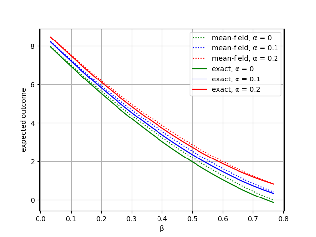
(a) $k=2$

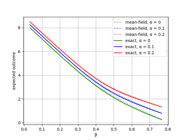
(b) $k=6$

Figure 3: For $k=2$ (left) and $k=6$ (right), the expected $\mathsf{GTFT}$ payoff functions for the $k$-IGT dynamics in the mean-field formulation of expression 46 (dotted lines) and the exact formulation with respect to the stationary distribution $\boldsymbol{\pi}$ (solid lines) on a population of $m=20$ $\mathsf{GTFT}$ nodes.

References

- [AAD+06] Dana Angluin, James Aspnes, Zoë Diamadi, Michael J. Fischer, and René Peralta. Computation in networks of passively mobile finite-state sensors. Distributed Comput., 18(4):235–253, 2006.
- [AAE08a] Dana Angluin, James Aspnes, and David Eisenstat. Fast computation by population protocols with a leader. Distributed Computing, 21(3):183–199, September 2008.
- [AAE08b] Dana Angluin, James Aspnes, and David Eisenstat. A simple population protocol for fast robust approximate majority. Distributed Computing, 21(2):87–102, 2008.
- [AAE+17] Dan Alistarh, James Aspnes, David Eisenstat, Rati Gelashvili, and Ronald L Rivest. Time-space trade-offs in population protocols. In Proceedings of the Twenty-Eighth Annual ACM-SIAM Symposium on Discrete Algorithms, pages 2560–2579. SIAM, 2017.
- [AAG18] Dan Alistarh, James Aspnes, and Rati Gelashvili. Space-optimal majority in population protocols. In Proceedings of the 29th ACM-SIAM Symposium on Discrete Algorithms, (SODA), pages 2221–2239, 2018.
- [AG15] Dan Alistarh and Rati Gelashvili. Polylogarithmic-time leader election in population protocols. In Automata, Languages, and Programming, pages 479–491. Springer, 2015.
- [AGV15] Dan Alistarh, Rati Gelashvili, and Milan Vojnović. Fast and exact majority in population protocols. In Proceedings of the 2015 ACM Symposium on Principles of Distributed Computing, pages 47–56, 2015.
- [AH81] Robert Axelrod and William D Hamilton. The evolution of cooperation. Science, 211(4489):1390–1396, 1981.
- [ALC+17] Benjamin Allen, Gabor Lippner, Yu-Ting Chen, Babak Fotouhi, Naghmeh Momeni, Shing-Tung Yau, and Martin A Nowak. Evolutionary dynamics on any population structure. Nature, 544(7649):227–230, 2017.
- [BCC+13] Olivier Bournez, Jérémie Chalopin, Johanne Cohen, Xavier Koegler, and Mikael Rabie. Population protocols that correspond to symmetric games. Int. J. Unconv. Comput., 9(1-2):5–36, 2013.
- [BCCK09] Olivier Bournez, Jérémie Chalopin, Johanne Cohen, and Xavier Koegler. Playing with population protocols. arXiv preprint arXiv:0906.3256, 2009.
- [BCM+18] Luca Becchetti, Andrea Clementi, Pasin Manurangsi, Emanuele Natale, Francesco Pasquale, Prasad Raghavendra, and Luca Trevisan. Average whenever you meet: Opportunistic protocols for community detection. In 26th Annual European Symposium on Algorithms, pages 1–13. Schloss Dagstuhl, 2018.
- [BCN+14] Luca Becchetti, Andrea Clementi, Emanuele Natale, Francesco Pasquale, and Riccardo Silvestri. Plurality consensus in the gossip model. In Proceedings of the twenty-sixth annual ACM-SIAM symposium on Discrete algorithms, pages 371–390. SIAM, 2014.
- [BCN20] Luca Becchetti, Andrea Clementi, and Emanuele Natale. Consensus dynamics: An overview. ACM SIGACT News, 51(1):58–104, 2020.
- [BFK+16] Petra Berenbrink, Tom Friedetzky, Peter Kling, Frederik Mallmann-Trenn, and Chris Wastell. Plurality consensus via shuffling: Lessons learned from load balancing. arXiv preprint arXiv:1602.01342, 2016.
- [BGK20] Petra Berenbrink, George Giakkoupis, and Peter Kling. Optimal time and space leader election in population protocols. In Proc. 52nd Annual ACM SIGACT Symposium on Theory of Computing (STOC 2020), pages 119–129, 2020.
- [BHP14] Riddhipratim Basu, Jonathan Hermon, and Yuval Peres. Characterization of cutoff for reversible markov chains. In Proceedings of the twenty-sixth annual ACM-SIAM symposium on Discrete algorithms, pages 1774–1791. SIAM, 2014.
- [Car10] Pierre Cardaliaguet. Notes on mean field games. Technical report, Technical report, 2010.
- [CBL06] Nicolo Cesa-Bianchi and Gábor Lugosi. Prediction, learning, and games. Cambridge university press, 2006.
- [CCDS17] Ho-Lin Chen, Rachel Cummings, David Doty, and David Soloveichik. Speed faults in computation by chemical reaction networks. Distributed Computing, 30(5):373–390, 2017.
- [CCG+11] Areski Cousin, Stéphane Crépey, Olivier Guéant, David Hobson, Monique Jeanblanc, Jean-Michel Lasry, Jean-Paul Laurent, Pierre-Louis Lions, Peter Tankov, Olivier Guéant, et al. Mean field games and applications. Paris-Princeton lectures on mathematical finance 2010, pages 205–266, 2011.
- [CD11] Yang Cai and Constantinos Daskalakis. On minmax theorems for multiplayer games. In Proceedings of the twenty-second annual ACM-SIAM symposium on Discrete algorithms, pages 217–234. SIAM, 2011.
- [CDS+13] Yuan-Jyue Chen, Neil Dalchau, Niranjan Srnivas, Andrew Phillips, Luca Cardelli, David Soloveichik, and Georg Seelig. Programmable chemical controllers made from dna. Nature Nanotechnology, 8(10):755–762, 2013.
- [CKL16] Luca Cardelli, Marta Kwiatkowska, and Luca Laurenti. Programming discrete distributions with chemical reaction networks. In Proceedings of the 22nd International Conference on DNA Computing and Molecular Programming, DNA22, pages 35–51. Springer, 2016.
- [DEG+22] David Doty, Mahsa Eftekhari, Leszek Gąsieniec, Eric Severson, Przemyslaw Uznański, and Grzegorz Stachowiak. A time and space optimal stable population protocol solving exact majority. In 2021 IEEE 62nd Annual Symposium on Foundations of Computer Science (FOCS), pages 1044–1055. IEEE, 2022.
- [Det94] Holger Dette. On a generalization of the ehrenfest urn model. Journal of applied probability, 31(4):930–939, 1994.
- [DGM90] Persi Diaconis, Ronald L. Graham, and John A. Morrison. Asymptotic analysis of a random walk on a hypercube with many dimensions. Random Structures & Algorithms, 1(1):51–72, 1990.
- [Dia11] Persi Diaconis. The mathematics of mixing things up. Journal of Statistical Physics, 144(3):445–458, 2011.
- [Dot14] David Doty. Timing in chemical reaction networks. In Proceedings of the Twenty-Fifth Annual ACM-SIAM Symposium on Discrete Algorithms, SODA ’14, pages 772–784. SIAM, 2014.
- [DS18] David Doty and David Soloveichik. Stable leader election in population protocols requires linear time. Distributed Computing, 31(4):257–271, 2018.
- [DV12] Moez Draief and Milan Vojnovic. Convergence speed of binary interval consensus. SIAM Journal on Control and Optimization, 50(3):1087–1109, 2012.
- [EEA07] Paul Ehrenfest and Tatjana Ehrenfest-Afanassjewa. Über zwei bekannte Einwände gegen das Boltzmannsche H-Theorem. Hirzel, 1907.
- [FJ06] Michael Fischer and Hong Jiang. Self-stabilizing leader election in networks of finite-state anonymous agents. In Principles of Distributed Systems, pages 395–409. Springer, 2006.
- [GNW16] George Giakkoupis, Yasamin Nazari, and Philipp Woelfel. How asynchrony affects rumor spreading time. In Proceedings of the 2016 ACM Symposium on Principles of Distributed Computing, pages 185–194, 2016.
- [GP16] Mohsen Ghaffari and Merav Parter. A polylogarithmic gossip algorithm for plurality consensus. In Proceedings of the 35th ACM Symposium on Principles of Distributed Computing, (PODC), pages 117–126, 2016.
- [GPD20] Noah Golowich, Sarath Pattathil, and Constantinos Daskalakis. Tight last-iterate convergence rates for no-regret learning in multi-player games. Advances in neural information processing systems, 33:20766–20778, 2020.
- [GS18] Leszek Gąsieniec and Grzegorz Stachowiak. Fast space optimal leader election in population protocols. In Proceedings of the 29th ACM-SIAM Symposium on Discrete Algorithms, (SODA), pages 2653–2667, 2018.
- [GS20] Geoffrey Grimmett and David Stirzaker. Probability and random processes. Oxford university press, 2020.
- [HNS13] Christian Hilbe, Martin A Nowak, and Karl Sigmund. Evolution of extortion in iterated prisoner’s dilemma games. Proceedings of the National Academy of Sciences, 110(17):6913–6918, 2013.
- [HS98] Josef Hofbauer and Karl Sigmund. Evolutionary games and population dynamics. Cambridge university press, 1998.
- [Kac47] Mark Kac. Random walk and the theory of brownian motion. The American Mathematical Monthly, 54(7P1):369–391, 1947.
- [KM65] Samuel Karlin and James McGregor. Ehrenfest urn models. Journal of Applied Probability, 2(2):352–376, 1965.
- [KS93] Olaf Krafft and Martin Schaefer. Mean passage times for tridiagonal transition matrices and a two-parameter ehrenfest urn model. Journal of Applied Probability, 30(4):964–970, 1993.
- [LHN05] Erez Lieberman, Christoph Hauert, and Martin A Nowak. Evolutionary dynamics on graphs. Nature, 433(7023):312–316, 2005.
- [LL07] Jean-Michel Lasry and Pierre-Louis Lions. Mean field games. Japanese journal of mathematics, 2(1):229–260, 2007.
- [LP17] David A Levin and Yuval Peres. Markov chains and mixing times, volume 107. American Mathematical Soc., 2017.
- [LZMJ20] Tianyi Lin, Zhengyuan Zhou, Panayotis Mertikopoulos, and Michael Jordan. Finite-time last-iterate convergence for multi-agent learning in games. In International Conference on Machine Learning, pages 6161–6171. PMLR, 2020.
- [Mar09] James AR Marshall. The donation game with roles played between relatives. Journal of Theoretical Biology, 260(3):386–391, 2009.
- [Mol85] Per Molander. The optimal level of generosity in a selfish, uncertain environment. Journal of Conflict Resolution, 29(4):611–618, 1985.
- [MU17] Michael Mitzenmacher and Eli Upfal. Probability and computing: Randomization and probabilistic techniques in algorithms and data analysis. Cambridge university press, 2017.
- [MVCS12] Luis A Martinez-Vaquero, Jose A Cuesta, and Angel Sanchez. Generosity pays in the presence of direct reciprocity: A comprehensive study of 2 2 repeated games. PLoS One, 7(4):e35135, 2012.
- [Now06] Martin A Nowak. Evolutionary dynamics: exploring the equations of life. Harvard university press, 2006.
- [NRTV07] Noam Nisan, Tim Roughgarden, Eva Tardos, and Vijay V Vazirani. Algorithmic game theory, 2007. Book available for free online, 2007.
- [NS92] Martin A Nowak and Karl Sigmund. Tit for tat in heterogeneous populations. Nature, 355(6357):250–253, 1992.
- [NS93] Martin Nowak and Karl Sigmund. A strategy of win-stay, lose-shift that outperforms tit-for-tat in the prisoner’s dilemma game. Nature, 364(6432):56–58, 1993.
- [OR94] Martin J Osborne and Ariel Rubinstein. A course in game theory. MIT press, 1994.
- [Owe13] Guillermo Owen. Game theory. Emerald Group Publishing, 2013.
- [PVV09] Etienne Perron, Dinkar Vasudevan, and Milan Vojnovic. Using three states for binary consensus on complete graphs. In INFOCOM 2009, IEEE, pages 2527–2535. IEEE, 2009.
- [Rob84] Axelrod Robert. The evolution of cooperation. Basic Books, 1984.
- [Sch21] Laura Schmid. Evolution of cooperation via (in) direct reciprocity under imperfect information. PhD thesis, 2021.
- [SHCN22] Laura Schmid, Christian Hilbe, Krishnendu Chatterjee, and Martin A Nowak. Direct reciprocity between individuals that use different strategy spaces. PLoS Computational Biology, 18(6):e1010149, 2022.
- [Smi82] John Maynard Smith. Evolution and the Theory of Games. Cambridge University Press, 1982.
- [SP13] Alexander J Stewart and Joshua B Plotkin. From extortion to generosity, evolution in the iterated prisoner’s dilemma. Proceedings of the National Academy of Sciences, 110(38):15348–15353, 2013.
- [Tak79] Lajos Takács. On an urn problem of paul and tatiana ehrenfest. In Mathematical Proceedings of the Cambridge Philosophical Society, volume 86, pages 127–130. Cambridge University Press, 1979.