SafeDreamer: Safe Reinforcement Learning with World Models

Abstract

The deployment of Reinforcement Learning (RL) in real-world applications is constrained by its failure to satisfy safety criteria. Existing Safe Reinforcement Learning (SafeRL) methods, which rely on cost functions to enforce safety, often fail to achieve zero-cost performance in complex scenarios, especially vision-only tasks. These limitations are primarily due to model inaccuracies and inadequate sample efficiency. The integration of world models has proven effective in mitigating these shortcomings. In this work, we introduce SafeDreamer, a novel algorithm incorporating Lagrangian-based methods into world model planning processes within the superior Dreamer framework. Our method achieves nearly zero-cost performance on various tasks, spanning low-dimensional and vision-only input, within the Safety-Gymnasium benchmark, showcasing its efficacy in balancing performance and safety in RL tasks. Further details and resources are available on the project website: https://sites.google.com/view/safedreamer.

1 Introduction

A challenge in the real-world deployment of RL agents is to prevent unsafe situations (Feng et al., 2023). SafeRL proposes a practical solution by defining a constrained Markov decision process (CMDP) (Altman, 1999) and integrating an additional cost function to quantify potential hazardous behaviors. In this process, agents aim to maximize rewards while maintaining costs below predefined constraint thresholds. Several remarkable algorithms have been developed on this foundation (Achiam et al., 2017; Yang et al., 2022; Hogewind et al., 2022).

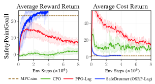
Figure 1: The performance of SafeDreamer in comparison to the baselines.

However, with the cost threshold nearing zero, existing Lagrangian-based methods often fail to meet constraints or meet them but cannot complete the tasks. Conversely, using an internal dynamics model, an agent can efficiently plan action trajectories to solve the problem. To tackel this issue, we compare the performance of the model-free SafeRL algorithm CPO (Achiam et al., 2017) with PPO-Lag (Ray et al., 2019) and the model-based RL approach MPC using a ground-truth simulator for online planning (Liu et al., 2020; Hansen et al., 2022) in the SafetyPointGoal1 environment (see Figure 1). The reward of CPO is consistently low, and the effectiveness of its cost reduction progressively diminishes. Conversely, the reward of PPO-Lag decreases as the cost reduces. These phenomena indicate that existing methods struggle to balance reward and cost. However, MPC converges to a nearly zero-cost while maintaining high reward, highlighting the importance of dynamics models and planning. However, obtaining a ground-truth simulator in complex scenarios like vision-only autonomous driving is impractical (Chen et al., 2022; Li et al., 2022). Additionally, the high expense of long-horizon planning forces optimization over a finite horizon, yielding temporally locally optimal and unsafe solutions. To fill such gaps, we aim to answer the following question:

How can we develop a safety-aware world model to balance long-term rewards and costs of agent?

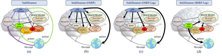
Figure 2: The Architecture of SafeDreamer. (a) illustrates all components of SafeDreamer, which distinguishes costs as safety indicators from rewards and balances them using the Lagrangian method and a safe planner. The OSRP (b) and OSRP-Lag (c) variants execute online safety-reward planning (OSRP) within the world models for action generation, especially OSRP-Lag integrates online planning with the Lagrangian approach to balance long-term rewards and costs. The BSRP-Lag variant of SafeDreamer (d) employs background safety-reward planning (BSRP) via the Lagrangian method within the world models to update a safe actor.

Autonomous Intelligence Architecture (LeCun, 2022) introduces a world model and utilizes scalar costs reflecting the discomfort level of the agent. Furthering this notion, several works (Hogewind et al., 2022; As et al., 2022; Jayant & Bhatnagar, 2022) proffer solutions to ensure safe and reward balance via world models. However, these methods fail to realize nearly zero-cost performance across several environments due to inaccuracies in modeling the agent’s safety in current or future states. In this work, we introduce SafeDreamer (as shown in Figure 2a), which integrates safety planning and the Lagrangian method within a world model to balance errors between cost models and critics. In summary, our contributions are:

• We present the online safety-reward planning algorithm (OSRP) (as shown in Figure 2b) and substantiate the feasibility of using online planning within world models to satisfy constraints in vision-only tasks. In particular, we employ the Constrained Cross-Entropy Method (Wen & Topcu, 2018) in the planning process.

• We integrate Lagrangian methods with the safety-reward online and background planning within world models to balance long-term reward and cost. This gives rise to two algorithms, OSRP-Lag and BSRP-Lag, as depicted in Figure 2c and 2d.

• SafeDreamer handles both low-dimensional and visual input tasks, achieving nearly zero-cost performance in the Safety-Gymnasium benchmark. We further illustrate that SafeDreamer outperforms competing model-based and model-free methods within this benchmark.

Owing to space constraints, the related work is provided in Appendix A.

2 Preliminaries

Constrained Markov Decision Process (CMDP)

SafeRL is often formulated as a CMDP $\mathcal{M}=(\mathcal{S},\mathcal{A},\mathbb{P},R,\mathcal{C},\mu,\gamma)$ (Altman, 1999; Sutton & Barto, 2018). The state and action spaces are $\mathcal{S}$ and $\mathcal{A}$, respectively. Transition probability $\mathbb{P}(s^{\prime}|s,a)$ refers to transitioning from $s$ to $s^{\prime}$ under action $a$. $R(s^{\prime}|s,a)$ stands for the reward acquired upon transitioning from $s$ to $s^{\prime}$ through action $a$. The cost function set $\mathcal{C}=\{(C_{i},b_{i})\}_{i=1}^{m}$ encompasses cost functions $C_{i}:\mathcal{S}\times\mathcal{A}\rightarrow\mathbb{R}$ and cost thresholds $b_{i},i=1,\cdots,m$. The initial state distribution and the discount factor are denoted by $\mu(\cdot):\mathcal{S}\rightarrow[0,1]$ and $\gamma\in(0,1)$, respectively. A stationary parameterized policy $\pi_{\theta}$ represents the action-taking probability $\pi_{\theta}(a|s)$ in state $s$. All stationary policies are represented as $\Pi_{\theta}=\{\pi_{\theta}:\theta\in\mathbb{R}^{p}\}$, where $\theta$ is the learnable network parameter. We define the infinite-horizon reward function and cost function as $J^{R}(\pi_{\theta})$ and $J^{C}_{i}(\pi_{\theta})$, respectively, as follows:

Figure 3: Safety-reward planning process. The agent acquires an observation and employs the encoder to distill it into a latent state $s_{1}$. Subsequently, the agent generates action trajectories by using policy and executes them within world models, predicting latent rollouts of the model state and a reward, cost, value, and cost value with each latent state. We employ TD($\lambda$) (Hafner et al., 2020) to estimate the return and the cost return for each trajectory that are used to update the policy via Equation 7.

$$J^{R}(\pi_{\theta})=\mathbb{E}\big{[}\sum_{t=0}^{\infty}\gamma^{t}R(s_{t+1}|s_{t},a_{t})|s_{0}\sim\mu,a_{t}\sim\pi_{\theta}\big{]}$$ (1)

$$J^{C}_{i}(\pi_{\theta})=\mathbb{E}\big{[}\sum_{t=0}^{\infty}\gamma^{t}C_{i}(s_{t+1}|s_{t},a_{t})|s_{0}\sim\mu,a_{t}\sim\pi_{\theta}\big{]}$$ (2)

The goal of CMDP is to achieve the optimal policy:

$$\pi_{\star}=\mathop{\arg\max}\limits_{\pi_{\theta}\in\Pi_{\mathcal{C}}}J^{R}(\pi_{\theta})$$ (3)

where $\Pi_{\mathcal{C}}=\Pi_{\theta}\cap\{\cap_{i=1}^{m}J^{C}_{i}(\pi_{\theta})\leq b_{i}\}$ denotes the feasible set of policies.

Safe Model-based RL Problem

We formulate a Safe Model-based RL problem as follows:

$$\max_{\pi_{\theta}\in\Pi_{\theta}}J^{R}_{\phi}(\pi_{\theta})~{}~{}~{}\text{s.t.}~{}~{}~{}J_{\phi}^{C}(\pi_{\theta})\leq b$$ (4)

$$J_{\phi}^{R}(\pi_{\theta})=\mathbb{E}\Big{[}\sum_{t=0}^{\infty}\gamma^{t}R(s_{t+1}|s_{t},a_{t})|s_{0}\sim\mu,s_{t+1}\sim\mathbb{P}_{\phi}(\cdot|s_{t},a_{t}),a_{t}\sim\pi_{\theta}\Big{]}$$ (5)

$$J_{\phi}^{C}(\pi_{\theta})=\mathbb{E}\Big{[}\sum_{t=0}^{\infty}\gamma^{t}C(s_{t+1}|s_{t},a_{t})|s_{0}\sim\mu,s_{t+1}\sim\mathbb{P}_{\phi}(\cdot|s_{t},a_{t}),a_{t}\sim\pi_{\theta}\Big{]}$$ (6)

In the above, $\mathbb{P}_{\phi}(\cdot|s_{t},a_{t})$ is a $\phi$-parameterized world model, we assume the initial state $s_{0}$ is sampled from the true initial state distribution $\mu$ and $s_{t+1}\sim\mathbb{P}_{\phi}(\cdot|s_{t},a_{t}),\forall t>0$. We would use the world model $\mathbb{P}_{\phi}$ to roll out imaginary trajectories and then estimate their reward returns and cost returns required for policy optimization algorithms. Without loss of generality, we will restrict our discussion to the case of one constraint with a cost function $C$ and a cost threshold $b$.

3 Methods

In this section, we introduce SafeDreamer, a framework for integrating safety-reward planning of the world models with the Lagrangian methods to balance rewards and costs. The world model is trained through a replay buffer of past experiences as the agent interacts with the environment. Meanwhile, we elucidate the notation for our safe model-based agent, assuming access to learned world models, which generate latent rollouts for online or background planning, depicted in Figure 3. The design and training objectives of these models are described in Section 4.

3.1 Model Components

SafeDreamer includes world models and actor-critic models. At each time step, world models receive an observation $o_{t}$ and an action $a_{t}$. The observation is condensed into a discrete representation $z_{t}$. Then, $z_{t}$, along with the action, are used by the sequence model to predict the next representation $\hat{z}_{t+1}$. We represent the model state $s_{t}=\{h_{t},z_{t}\}$ by concatenating $h_{t}$ and $z_{t}$, where $h_{t}$ is a recurrent state. Decoders employ $s_{t}$ to predict observations, rewards, and costs. Meanwhile, $s_{t}$ serves as the input of the actor-critic models to predict reward value $v_{r_{t}}$, cost value $v_{c_{t}}$, and action $a_{t}$. This notation offers our model components:

$$\begin{split}\begin{array}[]{ll}\text{Observation encoder:}&z_{t}\sim E_{\phi}\left(z_{t}\mid h_{t},o_{t}\right)\\ \text{Observation decoder:}&\hat{o}_{t}\sim O_{\phi}\left(\hat{o}_{t}\mid s_{t}\right)\\ \text{Reward decoder:}&\hat{r}_{t}\sim R_{\phi}\left(\hat{r}_{t}\mid s_{t}\right)\\ \text{Cost decoder:}&\hat{c}_{t}\sim C_{\phi}\left(\hat{c}_{t}\mid s_{t}\right)\\ \end{array}\end{split}\;\begin{split}\begin{array}[]{ll}\text{Sequence model:}&h_{t},\hat{z}_{t}=S_{\phi}\left(h_{t-1},z_{t-1},a_{t-1}\right)\\ \text{Actor:}&a_{t}\sim\pi_{\theta}(a_{t}\mid s_{t})\\ \text{Reward critic:}&\hat{v}_{r_{t}}\sim V_{\psi_{r}}(\hat{v}_{r_{t}}\mid s_{t})\\ \text{Cost critic:}&\hat{v}_{c_{t}}\sim V_{\psi_{c}}(\hat{v}_{c_{t}}\mid s_{t})\\ \end{array}\end{split}$$

3.2 Online Safety-Reward Planning (OSRP) via World Models

1 Input: current model state $s_{t}$, planning horizon $H$,

2 num sample/policy/safe trajectories $N_{\pi_{\mathcal{N}}},N_{\pi_{\theta}},N_{s}$,

3 Lagrangian multiplier $\lambda_{p}$, cost limit $b$, $\mu^{0},\sigma^{0}$ for $\mathcal{N}$

4 for $j\leftarrow 1$ to J do

5       Init. empty safe/candidate/elite actions set $A_{s},A_{c},A_{e}$

6       Sample $N_{\pi_{\mathcal{N}}}+N_{\pi_{\theta}}$ traj. $\{s_{i},a_{i},s_{i+1}\}_{i=t}^{t+H}$ using $\mathcal{N}(\mu^{j-1},(\sigma^{j-1})^{2}\mathrm{I})$, $\pi_{\theta}$ within $S_{\phi}$ with $s_{t}$ as the initial state

7      

8      for all $N_{\pi_{\mathcal{N}}}+N_{\pi_{\theta}}$ trajectories do

9             Init. trajectory cost $J_{\phi}^{C,H}\left(\pi\right)\leftarrow 0$

10             for $t\leftarrow H$ to 1 do

11                   Compute $R^{\lambda}(s_{t}),C^{\lambda}(s_{t})$ via Equation (8)

12                   $J_{\phi}^{C,H}\leftarrow\gamma J_{\phi}^{C,H}+C_{\phi}(s_{t})$

13                  

14             end for

15            $J_{\phi}^{R}$, $J_{\phi}^{C}\leftarrow R^{\lambda}(s_{1})$, $C^{\lambda}(s_{1})$

16             $J_{\phi}^{C^{\prime}}\leftarrow(J_{\phi}^{C,H}/H)L$

17             if $J_{\phi}^{C^{\prime}}<b$ then

18                   $A_{s}\leftarrow A_{s}\cup\{a_{t:t+H}\}$

19                  

20             end if

21            

22       end for

23      

24      if $|A_{s}|<N_{s}$ then

25             $\Omega=-J_{\phi}^{C^{\prime}},A_{c}=\{a_{t:t+H}\}_{i=1}^{N_{\pi_{\mathcal{N}}}+N_{\pi_{\theta}}}$

26            

27      else

28             $\Omega=J_{\phi}^{R},A_{c}=A_{s}$

29             $\Omega=J_{\phi}^{R}-\lambda_{p}J_{\phi}^{C},A_{c}=A_{s}$

30       end if

31      Select the top-k action trajectories with highest $\Omega$ values among $A_{c}$ as elite actions $A_{e}$

32       $\mu^{j},\sigma^{j}=\mathrm{MEAN}\left(A_{e}\right),\mathrm{STD}\left(A_{e}\right)$

33      

34 end for

Return: $a\sim\mathcal{N}(\mu^{J},(\sigma^{J})^{2}\mathrm{I})$

Red is OSRP only and green is OSRP-Lag only.

Algorithm 1 Online Safety-Reward Planning.

Red is OSRP only and green is OSRP-Lag only.

SafeDreamer (OSRP) We introduce online safety-reward planning (OSRP) through world models, depicted in Figure 2b. The online planning procedure is conducted at every decision time $t$, generating state-action trajectories from the current state $s_{t}$ within the world model. Each trajectory is evaluated by learned reward and cost models, along with their critics, and the optimal safe action trajectory is selected for execution in the environment. Specifically, we adopt the Constrained Cross-Entropy Method (CCEM) (Wen & Topcu, 2018) for planning. To commence this process, we initialize $(\mu^{0},\sigma^{0})_{t:t+H}$, with $\mu^{0},\sigma^{0}\in\mathbb{R}^{|\mathcal{A}|}$, which represent a sequence of action mean and standard deviation spanning over the length of planning horizon $H$. Following this, we independently sample $N$ state trajectories using the current action distribution $\mathcal{N}(\mu^{j-1},\sigma^{j-1})$ at iteration $j-1$ within the world model. Afterward, we estimate the reward return $J_{\phi}^{R}$ and cost return $J_{\phi}^{C}$ of each trajectory, as highlighted in blue in Algorithm 1. The estimation of $J_{\phi}^{R}$ is obtained using the TD$(\lambda)$ value of reward, denoted as $R^{\lambda}$, which balances the bias and variance of the critics through bootstrapping and Monte Carlo value estimation (Hafner et al., 2023). The total cost over $H$ steps, denoted as $J_{\phi}^{C,H}$, is computed using the cost model $C_{\phi}$: $J_{\phi}^{C,H}=\sum_{t}^{t+H}\gamma^{t}C_{\phi}(s_{t})$. We use TD$(\lambda)$ value of cost $C^{\lambda}$ to estimate $J_{\phi}^{C}$ and define $J_{\phi}^{C^{\prime}}=(J_{\phi}^{C,H}/H)L$ as an alternative estimation for avoiding errors of the cost critic, where $L$ signifies the episode length. Concurrently, we set the criterion for evaluating whether a trajectory satisfies the cost threshold $b$ as $J_{\phi}^{C^{\prime}}<b$. We use $|A_{s}|$ to denote the number of trajectories that meet the cost threshold and represent the desired number of safe trajectories as $N_{s}$. Upon this setup, one of the following two conditions will hold:

1. If $|A_{s}|<N_{s}$: We employ $-J_{\phi}^{C^{\prime}}$ as the sorting key $\Omega$. The complete set of sampled action trajectories serves as the candidate action set $A_{c}$.

2. If $|A_{s}|\geq N_{s}$: We adopt $J_{\phi}^{R}$ as the sorting key $\Omega$ for SafeDreamer (OSRP), and $J_{\phi}^{R}-\lambda_{p}J_{\phi}^{C}$ for SafeDreamer (OSRP-Lag), highlighted in red and green, respectively, in Algorithm 1, with further discussion in Section 3.3. The safe action trajectory set $A_{s}$ is selected as the candidate actions set $A_{c}$.

We select the top-$k$ action trajectories, those with the highest $\Omega$ values, from the candidate action set $A_{c}$ to be the elite actions $A_{e}$. Subsequently, we obtain new parameters $u^{j}$ and $\sigma^{j}$ at iteration $j$: $\mu^{j}=\frac{1}{k}\sum_{i=1}^{k}A_{e}^{i}$, $\sigma^{j}=\sqrt{\frac{1}{k}\sum_{i=1}^{k}(A_{e}^{i}-u^{j})^{2}}$. The planning process is concluded after reaching a predetermined number of iterations $J$. An action trajectory is sampled from the final distribution $\mathcal{N}(\mu^{J},(\sigma^{J})^{2}\mathrm{I})$. Subsequently, the first action from this trajectory is executed in the real environment.

3.3 Lagrangian Method with World Models Planning

The Lagrangian method stands as a general solution for SafeRL, and the commonly used ones are Augmented Lagrangian (Dai et al., 2023) and PID Lagrangian (Stooke et al., 2020). However, it has been observed that employing Lagrangian approaches for model-free SafeRL results in suboptimal performance under low-cost threshold settings, attributable to inaccuracies in the critic’s estimation. This work integrates the Lagrangian method with online and background planning phases to balance errors between cost models and critics. By adopting the relaxation technique of the Lagrangian method (Nocedal & Wright, 2006), the Equation (4) is transformed into an unconstrained safe model-based optimization problem, where $\lambda_{p}$ is the Lagrangian multiplier:

$$\underset{\pi_{\theta}\in\Pi_{\theta}}{\max}\ \underset{\bm{\lambda_{p}}\geq 0}{\min}\ J_{\phi}^{R}\left(\pi_{\theta}\right)-\lambda_{p}\left(J_{\phi}^{C}\left(\pi_{\theta}\right)-b\right)$$ (7)

SafeDreamer (OSRP-Lag) We introduced the PID Lagrangian method (Stooke et al., 2020) into our online safety-reward planning scheme, yielding SafeDreamer (OSRP-Lag), as shown in Figure 2c. In the online planning process, the sorting key $\Omega$ is determined by $J_{\phi}^{R}-\lambda_{p}J_{\phi}^{C}$ when $\left|A_{s}\right|\geq N_{s}$, denoted in green in Algorithm 1, where $J_{\phi}^{C}$ is approximated using the TD($\lambda$) value of cost, denoted as $C^{\lambda}$, computed with $V_{\psi_{c}}$ and $C_{\phi}$:

$$C^{\lambda}(s_{t})=\begin{cases}C_{\phi}(s_{t})+\gamma\left((1-\lambda)V_{\psi_{c}}\left(s_{t+1}\right)+\lambda C^{\lambda}(s_{t+1})\right)&\text{ if }\quad t<H\\ V_{\psi_{c}}\left(s_{t}\right)&\text{ if }\quad t=H\end{cases}$$ (8)

The intuition of OSRP-Lag is to optimize a conservative policy under comparatively safe conditions, considering long-term risks. The process for updating the Lagrangian multiplier remains consistent with Stooke et al. (2020) and depends on the episode cost encountered during the interaction between agent and environment. Refer to Algorithm 3 for additional details.

SafeDreamer (BSRP-Lag) We use the Lagrangian method in background safety-reward planning (BSRP) for the safe actor training, which is referred to as SafeDreamer (BSRP-Lag), as shown in Figure 2d. During the actor training, we produce imagined latent rollouts of length $T=15$ within world models in the background. We begin with observations from the replay buffer, sampling actions from the actor, and observations from the world models. The world models also predict rewards and costs, from which we compute TD($\lambda$) value $R^{\lambda}(s_{t})$ and $C^{\lambda}(s_{t})$. These values are then utilized in stochastic backpropagation (Hafner et al., 2023) to update the safe actor, a process we denominate as background safety-reward planning. The training loss in this process guides the safe actor to maximize expected return and entropy while minimizing cost return, utilizing the Augmented Lagrangian method (Simo & Laursen, 1992; As et al., 2022):

$$\mathcal{L}(\theta)=-\sum_{t=1}^{T}\operatorname{sg}\left(R^{\lambda}(s_{t})\right)+\eta\mathrm{H}\left[\pi_{\theta}\left(a_{t}\mid s_{t}\right)\right]-\Psi\left(sg(C^{\lambda}(s_{t})),\lambda_{p}^{k},\mu^{k}\right)$$ (9)

Here, $sg(\cdot)$ represents the stop-gradient operator of world models and critics, $\mu^{k}=\max(\mu^{k-1}(\nu+1.0),1.0)$ represents a non-decreasing term that corresponds to the current gradient step $k$, $\nu>0$. Define $\Delta=\left(C^{\lambda}(s_{t})-b\right)$. The update rules for the penalty term in the training loss and the Lagrangian multiplier are as follows:

$$\Psi\left(sg(C^{\lambda}(s_{t})),\lambda_{p}^{k},\mu^{k}\right),\lambda_{p}^{k+1}=\begin{cases}\lambda_{p}^{k}\Delta+\frac{\mu^{k}}{2}\Delta^{2},\lambda_{p}^{k}+\mu^{k}\Delta&\text{ if }\lambda_{p}^{k}+\mu^{k}\Delta\geq 0\\ -\frac{\left(\lambda_{p}^{k}\right)^{2}}{2\mu^{k}},0&\text{ otherwise }\end{cases}$$ (10)

Input: batch length $T$, batch size $B$, episode length $L$, initial Lagrangian multiplier $\lambda_{p}$

1 Initialize the world models parameters $\phi$, actor-critic parameters $\theta,V_{\psi_{r}},V_{\psi_{c}}$

2 Initialize dataset $\mathcal{D}$ using a random policy

3 while not converged do

4       Sample $B$ trajectories $\{o_{t},a_{t},o_{t+1},r_{t+1},c_{t+1}\}_{t:t+T}\sim\mathcal{D}$

5       Update the world models via minimize Equation (11)

6       Condense $o_{t:t+T}$ into $s_{t:t+T}$ via world models

7       Generate latent rollouts using the actor within the world model with $s_{t:t+T}$ as the initial state

8       Update the reward and cost critics via minimize Equation (13)

       Update the safe actor and $\lambda_{p}$ via Equation (9) and Equation (10)

        // Only BSRP-Lag

9       $\mathcal{J}_{\mathcal{C}}\leftarrow 0$

10       for $t=1$ to $L$ do

11             Condense $o_{t}$ into latent state via ${s}_{t}\sim S_{\phi}(o_{t},s_{t-1},a_{t-1})$

             Sample $a_{t}\sim\pi_{a}(\cdot|s_{t})$

              // Only BSRP-Lag

             Sample $a_{t}\sim Planner(s_{t},\lambda_{p})$

              // Only OSRP-Lag or OSRP

12             Execute action $a_{t}$, observe $o_{t+1},r_{t+1},c_{t+1}$ returned from the environment

13             Update dataset $\mathcal{D}\leftarrow\mathcal{D}\cup\left\{o_{t},a_{t},o_{t+1},r_{t+1},c_{t+1}\right\}$

14             $\mathcal{J}_{\mathcal{C}}\leftarrow\mathcal{J}_{\mathcal{C}}+c_{t+1}$

15            

16       end for

       Use $\mathcal{J}_{\mathcal{C}}$ to update $\lambda_{p}$ via Algorithm 3

        // Only OSRP-Lag

17      

18 end while

Algorithm 2   SafeDreamer. Color green is OSRP-Lag or OSRP, purple is BSRP-Lag

4 Practical Implementation

Leveraging the framework above, we develop SafeDreamer, a safe model-based RL algorithm that extends the architecture of DreamerV3 (Hafner et al., 2023).

World Model Implementation The world model, trained via a variational auto-encoding (Kingma & Welling, 2013), transforms observations $o_{t}$ into latent representations $z_{t}$. These representations are used in reconstructing observations, rewards, and costs, enabling the evaluation of reward and safety of action trajectories during planning. The representations $z_{t}$ are regularized towards a prior by a regularization loss, ensuring the representations are predictable. We utilize the predicted distribution over $\hat{z}_{t}$ from the sequence model as this prior. Meanwhile, we utilize representation $z_{t}$ as a posterior, and the future prediction loss trains the sequence model to leverage historical information from times before $t$ to construct a prior approximating the posterior at time $t$. The observation, reward, and cost decoders are trained by optimizing the log-likelihood:

$$\mathcal{L}(\phi)= \sum_{t=1}^{T}\underbrace{\alpha_{q}\operatorname{KL}\left[z_{t}\;\|\;\operatorname{sg}(\hat{z}_{t})\right]}_{\text{regularization loss}}+\underbrace{\alpha_{p}\mathrm{KL}\left[\operatorname{sg}(z_{t})\;\|\;\hat{z}_{t}\right]}_{\text{future prediction loss}}$$ (11)

$$-\underbrace{\beta_{o}\ln O_{\phi}\left(o_{t}\mid s_{t}\right)}_{\text{observation loss}}-\underbrace{\beta_{r}\ln R_{\phi}\left(r_{t}\mid s_{t}\right)}_{\text{reward loss}}-\underbrace{\beta_{c}\ln C_{\phi}\left(c_{t}\mid s_{t}\right)}_{\text{cost loss}}$$

Here, $sg(\cdot)$ is the stop-gradient operator. The world models are based on the Recurrent State Space Model (RSSM) (Hafner et al., 2019b), utilizing GRU (Cho et al., 2014) for sequence modeling.

The SafeDreamer algorithm Algorithm 2 illustrates how the introduced components interrelate to build a safe model-based agent. We sample a batch of $B$ sequences of length $L$ from a replay buffer to train the world model during each update. In SafeDreamer (OSRP and OSRP-Lag), the actor aims to maximize the reward and the entropy to guide the planning process, which avoids excessively conservative policy. Specifically, SafeDreamer (BSRP-Lag) utilizes the safe actor for action generation during exploration to expedite decision time, bypassing online planning. See Appendix B for the design of critics and additional details.

5 Experimental Results

This section addresses the following issues: (1). How does SafeDreamer compare to existing safe model-free algorithms? (2). How does SafeDreamer against safe model-based algorithms? (3). Does SafeDreamer excel in visual and low-dimensional input environments?

5.1 Tasks Specification

We use different robotic agents in Safety-Gymnasium (Ji et al., 2023), which includes all tasks in Safety-Gym (Ray et al., 2019). The goal in both environments is to navigate robots to predetermined locations while avoiding collisions with hazards and vases. We evaluate algorithms using five fundamental environments (refer to Figure 17). The agent receives 64$\times$64 egocentric images or low-dimensional sensor inputs. Performance is assessed using metrics from Ray et al. (2019):

• Average undiscounted return over $E$ episodes: $\hat{J}(\pi)=\frac{1}{E}\sum_{i=1}^{E}\sum_{t=0}^{T_{\text{ep}}}r_{t}$

• Average undiscounted cost return over $E$ episodes: $\hat{J}_{c}(\pi)=\frac{1}{E}\sum_{i=1}^{E}\sum_{t=0}^{T_{\text{ep}}}c_{t}$

• Average cost throughout the entire training phase, namely the cost rate: Given a total of $T$ interaction steps, we define the cost rate $\rho_{c}(\pi)=\frac{\sum_{t=0}^{T}c_{t}}{T}$.

We calculate $\hat{J}(\pi)$ and $\hat{J}_{c}(\pi)$ by averaging episode costs and rewards over $E=10$ episodes, each of length $T_{\text{ep}}=1000$, without network updates. Unlike other metrics, $\rho_{c}(\pi)$ is calculated using costs incurred during training, not evaluation. Details are in Appendix E.

5.2 Comparisons

We compare SafeDreamer with other SafeRL algorithms. For further hyperparameter configurations and experiments, refer to Appendix C and D, respectively. The baselines include: (1). PPO-Lag, TRPO-Lag (Ray et al., 2019) (Model-free): Lagrangian versions of PPO and TRPO. (2). CPO (Achiam et al., 2017) (Model-free): A policy search algorithm with near-constraint satisfaction guarantees. (3). Safe SLAC (Hogewind et al., 2022) (Model-based): Combines SLAC (Lee et al., 2020) with the Lagrangian methos. (4). LAMBDA (As et al., 2022) (Model-based): Implemented in DreamerV1, combines Bayesian and Lagrangian methods. (5). MPC (Wen & Topcu, 2018; Liu et al., 2020) (Model-based): Employs CCEM for MPC with a ground-truth simulator, termed MPC:sim. Considering the intensive computational demands of the simulator, we set the planning horizon to 15, sample 150 trajectories, and optimize for 6 iterations. (6). MBPPO-Lag (As et al., 2022) (Model-based): Trains the policy through background planning using ensemble Gaussian models, serving as a model-based adaptation of PPO-Lag. (7). DreamerV3 (As et al., 2022) (Model-based): A model-based algorithm that integrates practical techniques and excels across domains

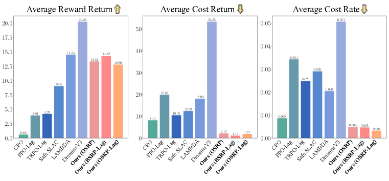
Figure 4: Experimental results from the five tasks. The results for the model-based methods are recorded after the agent completes 1M environment steps for SafetyPointGoal1 and SafetyRacecarGoal1, and 2M steps for SafetyPointButton1, SafetyPointPush2, and SafetyPointGoal2 environments, respectively. We follow the experimental procedures described by Ray et al. (2019) and conduct training for 8M steps for model-free algorithms.

5.3 Results

The results of our experiments are shown in Figure 4. We observe that SafeDreamer surpasses existing model-free methods, notably outperforming CPO by 20$\times$, PPO-Lag by 2.3$\times$, and TRPO-Lag by over 2$\times$, while reducing costs by 75.5%, 89.9%, and 80.9% respectively. Meanwhile, SafeDreamer attains rewards similar to model-based RL methods like LAMBDA, with a substantial 90.5% reduction in costs. Additionally, we find that SafeDreamer (OSRP-Lag) exhibits 33.3% and 30.4% reductions in cost rate compared to OSRP and BSRP-Lag, respectively, indicating that incorporating the Lagrangian method in online planning enhances safety during the training process.

Swift Convergence to Nearly Zero-cost As illustrated in Figure 5, SafeDreamer surpasses model-free algorithms regarding both rewards and costs. Although model-free algorithms can decrease costs over time, they struggle to achieve higher rewards. This challenge stems from their reliance on learning a policy purely through trial-and-error, devoid of world model assistance, which hampers optimal solution discovery with limited data samples. In Safety-Gymnasium tasks, the agent begins in a safe region at episode reset without encountering obstacles. A feasible solution apparent to humans is to keep the agent stationary, preserving its position. However, even with this simplistic policy, realizing zero-cost with model-free algorithms either demands substantial updates or remains elusive in some tasks.

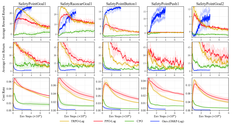
Figure 5: Metrics for our method and model-free baselines across five image-based safety tasks.

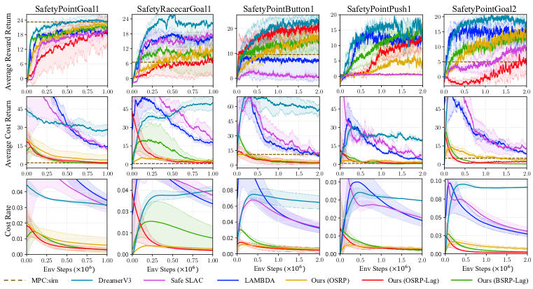
Figure 6: Comparing SafeDreamer to model-based baselines across five image-based safety tasks.

Dual Objective Realization: Balancing Enhanced Reward with Minimized Cost As depicted in Figure 6, SafeDreamer uniquely attains minimal costs while achieving higher rewards in the five visual-only safety tasks. In contrast, model-based algorithms such as LAMBDA and Safe SLAC attain a cost limit beyond which further reductions are untenable due to the inaccuracies of the world models. On the other hand, in environments with denser or more dynamic obstacles, such as SafetyPointGoal2 and SafetyPointButton1, MPC struggles to ensure safety due to the absence of a cost critic within a limited online planning horizon. Integrating a world model with critics enables agents to effectively utilize information on current and historical states to ensure their safety. From the beginning of training, our algorithms demonstrate safety behavior, ensuring extensive safe exploration. Specifically, in the SafetyPointGoal1 and SafetyPointPush1 environments, SafeDreamer matches the performance of DreamerV3 in reward while preserving nearly zero-cost.

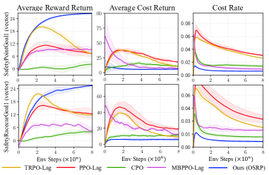
Figure 7: Comparing SafeDreamer to other baselines in low-dimensional input tasks.

Mastering Diverse Tasks in Visual and Low-dimensional Tasks We conducted evaluations within two low-dimensional sensor input environments, namely SafetyPointGoal1 (vector) and SafetyRacecarGoal1 (vector) (refer to Figure 7). The reward of MBPPO-Lag ceases to increase when the cost begins to decrease, similar to the phenomenon observed in PPO-Lag. Distinctly, our algorithm optimizes rewards while concurrently achieving a substantial cost reduction. Our results highlight our contribution in revealing the potential of planning within a word model to achieve exceptional results within the Safety-Gymnasium benchmark.

6 Conclusion

In this study, we tackle the issue of zero-cost performance within SafeRL, with the objective of finding a policy that maximizes return while ensuring minimal cost after training. We introduce SafeDreamer, a safe model-based RL algorithm that utilizes safety-reward planning of world models and the Lagrangian methods to balance long-term rewards and costs. SafeDreamer surpasses previous methods by achieving higher rewards and lower costs, demonstrating superior performance in tasks with low-dimensional and visual inputs. To our knowledge, SafeDreamer is the first algorithm to achieve nearly zero-cost in final performance, utilizing vision-only input in the Safety-Gymnasium benchmark. However, SafeDreamer trains each task independently, incurring substantial costs with each individual task. Future research should leverage offline data from multiple tasks to pre-train the world models, examining its ability to facilitate the safe exploration of new tasks.

Reproducibility Statement: All SafeDreamer agents are trained on one Nvidia 3090Ti GPU each and all experiments are conducted utilizing the Safety-Gymnasium benchmark. The source code and other results are available on the project website: https://sites.google.com/view/safedreamer. We implemented the baseline algorithm based on the following code repository: LAMBDA, Safe SLAC, and MBPPO-Lag, Dreamerv3, respectively. We further included additional baseline algorithms: CPO, TRPO-L, and PPO-L, sourced from the Omnisafe. For additional hyperparameter configurations and experiments, please refer to Appendix C.

Appendix A Related Work

Safe Reinforcement Learning SafeRL aims to manage optimization objectives under constraints, maintaining RL agent actions within prescribed safe threshold (Altman, 1999; Garcıa & Fernández, 2015). CPO (Achiam et al., 2017) offers the first general-purpose policy search algorithm for SafeRL, ensuring adherence to near-constraints iteratively. Nevertheless, second-order methods like CPO and PCPO (Yang et al., 2020) impose considerable computational costs due to their dependence on second-order information. First-order methods, such as FOCOPS (Zhang et al., 2020) and CUP (Yang et al., 2022), are designed to circumvent these challenges, delivering superior results by mitigating approximation errors inherent in Taylor approximations and inverting high-dimensional Fisher information matrices. Despite these advances, our experiments reveal that the convergence of safe model-free algorithms still requires substantial interaction with the environment, and model-based methods can effectively boost sample efficiency.

Safe Model-based RL Model-based RL (MBRL) approaches (Polydoros & Nalpantidis, 2017) serve as promising alternatives for modeling environment dynamics, categorizing into online planning—utilizing the world model for action selection (Hafner et al., 2019b; Camacho et al., 2007), and background planning—leveraging the world model for policy updates (Hafner et al., 2019a). Notably, methods like model predictive control (MPC) (Camacho et al., 2007) and Constrained Cross-Entropy Method (CCEM) (Wen & Topcu, 2018) exemplify online planning by ensuring action safety (Koller et al., 2018; Wabersich & Zeilinger, 2021; Liu et al., 2020), though this can lead to short-sighted decisions due to the limited scope of planning and absence of critics. Recent progress in MBRL seeks to embed terminal value functions into online model planning, fostering consideration of long-term rewards (Sikchi et al., 2022; Hansen et al., 2022; Moerland et al., 2023), but not addressing long-term safety. On the other hand, background planning methods like those in (Jayant & Bhatnagar, 2022; Thomas et al., 2021) employ ensemble Gaussian models and safety value functions to update policy with PPO (Schulman et al., 2017) and SAC (Haarnoja et al., 2018), respectively. However, challenges remain in adapting to vision input tasks. In this regard, the LAMBDA (As et al., 2022) represents a key progression in visual SafeRL by extending the DreamerV1 architecture (Hafner et al., 2019a) with principles from the Lagrangian method (Boyd & Vandenberghe, 2004). However, the constraints intrinsic to DreamerV1 limit its efficacy due to disregarding necessary adaptive modifications to reconcile variances in signal magnitudes and ubiquitous instabilities within all model elements (Hafner et al., 2023). This original framework’s misalignment with online planning engenders suboptimal results and a deficiency in low-dimensional input, thereby greatly reducing the benefits of the world model. Meanwhile, Safe SLAC (Hogewind et al., 2022) integrates the Lagrangian mechanism into SLAC (Lee et al., 2020), achieving comparable performance to LAMBDA on vision-only tasks. Yet, it does not maximize the potential of the world models to augment safety, overlooking imaginary rollouts that could potentially enhance online or background planning. A detailed comparison with various algorithms can be found in Table 1.

Table 1: Comparison to prior works. We compare key components of SafeDreamer to prior model-based and model-free algorithms. Predominantly, contemporary algorithms are tailored for low-dimensional input, while only a subset supports vision input. Our approach accommodates both input modalities. Moreover, Lagrangian-based and planning-based constitute two predominant strands of SafeRL algorithms, which we consolidate into a unified framework.

Method	Vision Input	Low-dimensional Input	Lagrangian-based	Online Planning	Background Planning
CPO (Achiam et al., 2017)	X	✓	✓	X	X
PPO-L (Ray et al., 2019)	X	✓	✓	X	X
TRPO-L (Ray et al., 2019)	X	✓	✓	X	X
MBPPO-L (Jayant & Bhatnagar, 2022)	X	✓	✓	X	✓
LAMBDA (As et al., 2022)	✓	X	✓	X	✓
SafeLOOP (Sikchi et al., 2022)	X	✓	X	✓	X
Safe SLAC (Hogewind et al., 2022)	✓	X	✓	X	X
DreamerV3 (Hafner et al., 2023)	✓	✓	X	X	✓
SafeDreamer (ours)	✓	✓	✓	✓	✓

Appendix B Details of SafeDreamer Training Process

Input: Proportional coefficient $K_{p}$, integral coefficient $K_{i}$, differential coefficient $K_{d}$

1

2Initialize previous integral item: $I^{0}\leftarrow 0$

3 Initialize previous episode cost: $J_{C}^{0}\leftarrow 0$

4 while iteration $k$ continues do

5       Receive cost $J_{C}^{k}$

6       $P\leftarrow J_{C}^{k}-d$

7       $D\leftarrow max(0,J_{C}^{k}-J_{C}^{k-1})$

8       $I^{k}\leftarrow max(0,I^{k-1}+D)$

9       $\lambda_{p}\leftarrow max(0,K_{p}P+K_{i}I^{k}+K_{d}D)$

10       Return Lagrangian multiplier $\lambda_{p}$

11      

12 end while

Algorithm 3 PID Lagrangian (Stooke et al., 2020)

PID Lagrangian with Planning The safety planner might fail to ensure zero-cost when the required hazard detection horizon surpasses the planning horizon, in accordance with the constraint $(J_{\phi}^{C,H}/H)L<b$ during planning. To overcome this limitation, we introduced the PID Lagrangian method (Stooke et al., 2020) into our planning scheme for enhancing the safety of exploration, yielding SafeDreamer (OSRP-Lag).

Cost Threshold Settings Our empirical studies show that for all SafeDreamer variations, a cost threshold of 2.0 leads to consistent convergence towards nearly zero-cost. Notably, when the cost threshold is set at 1.0 or below, SafeDreamer(OSRP) and SafeDreamer(OSRP-Lag) both struggle to converge within the allotted time. In contrast, SafeDreamer(LAG) manages to operate with a zero-cost threshold on some tasks but requires extended periods to achieve convergence. As such, in our current experimental setup, the cost threshold is set to 2.0.

Reward-driven Actor A reward-driven actor is trained to guide the planning process, enhancing reward convergence. The actor loss aims to balance the maximization of expected reward and entropy. The gradient of the reward term is estimated using stochastic backpropagation (Hafner et al., 2023), whereas that of the entropy term is calculated analytically:

$$\mathcal{L}(\theta)=-\sum_{t=1}^{T}\operatorname{sg}\left(R_{t}^{\lambda}(s_{t})\right)+\eta\mathrm{H}\left[\pi_{\theta}\left(a_{t}\mid s_{t}\right)\right]$$ (12)

Reward and Cost Critics The sparsity and heterogeneous distribution of costs within the environment complicate the direct regression of these values, thereby presenting substantial challenges for the learning efficiency of the cost critic. Leveraging the methodology from (Hafner et al., 2023), we employ a trio of techniques for critic training: discrete regression, twohot encoded targets (Bellemare et al., 2017; Schrittwieser et al., 2020), and symlog smoothing (Hafner et al., 2023; Webber, 2012):

$$\mathcal{L}_{\mathrm{reward\_critic}}(\psi_{r}) =-\sum_{t=1}^{T}\operatorname{sg}\left(\operatorname{twohot}\left(\operatorname{symlog}\left(R_{t}^{\lambda}\right)\right)\right)^{T}\ln p_{\psi_{r}}\left(\cdot\mid s_{t}\right)$$ (13)

where the critic network output the Twohot softmax probability $p_{\psi}\left(b_{i}\mid s_{t}\right)$ and

$$\operatorname{twohot}(x)_{i}=\left\{\begin{array}[]{ll}\left|b_{k+1}-x\right|/\left|b_{k+1}-b_{k}\right|&\text{ if }i=n\\ \left|b_{k}-x\right|/\left|b_{k+1}-b_{k}\right|&\text{ if }i=n+1\\ 0&\text{ else }\end{array},\ n=\sum_{j=1}^{|B|}1_{(b_{j}<x)},\ B=[-20\ldots 20]\right.$$

We define the bi-symmetric logarithm function (Webber, 2012) as $\operatorname{symlog}(x)=\operatorname{sign}(x)\ln(|x|+1)$ and its inverse function, as $\operatorname{symexp}(x)=\operatorname{sign}(x)(\exp(|x|)-1)$. The cost critic loss, represented as $\mathcal{L}_{\mathrm{cost\_critic}}(\psi_{c})$, is calculated similarly, using TD($\lambda$) value of cost $C_{t}^{\lambda}$. Additionally, extending the principle of Onehot encoding to continuous values, Twohot encoding allows us to reconstruct target values after encoding:$v_{\psi}\left(s_{t}\right)=\operatorname{symexp}\left(p_{\psi}\left(\cdot\mid s_{t}\right)^{T}B\right)$. For further details, please refer to (Hafner et al., 2023).

Appendix C Hyperparameters

The SafeDreamer experiments were executed utilizing Python3 and Jax 0.3.25, facilitated by CUDA 11.7, on an Ubuntu 20.04.2 LTS system (GNU/Linux 5.8.0-59-generic x86 64) equipped with 40 Intel(R) Xeon(R) Silver 4210R CPU cores (operating at 240GHz), 251GB of RAM, and an array of 8 GeForce RTX 3090Ti GPUs.

Table 2: Hyperparameters for SafeDreamer. When addressing other safety tasks, we suggest tuning the initial Lagrangian multiplier, proportional coefficient, integral coefficient, and difference coefficient at various scales.

Name	Symbol	Value	Description
World Model
Number of laten		48
Classes per laten		48
Batch size	$B$	64
Batch length	$T$	16
Learning rate		$10^{-4}$
Coefficient of kl divergence in loss	$\alpha_{q}$, $\alpha_{p}$	0.1, 0.5
Coefficient of decoder in loss	$\beta_{o}$, $\beta_{r}$, $\beta_{c}$	1.0, 1.0, 1.0
Planner
Planning horizon	$H$	15
Number of samples	$N_{\pi_{\mathcal{N}}}$	500
Mixture coefficient	$M$	0.05	$N_{\pi_{\theta}}=M*N_{\pi_{\mathcal{N}}}$
Number of iterations	$J$	6
Initial variance	$\sigma_{0}$	1.0
PID Lagrangian
Proportional coefficient	$K_{p}$	0.01
Integral coefficient	$K_{i}$	0.1
Differential coefficient	$K_{d}$	0.01
Initial Lagrangian multiplier	$\lambda_{p}^{0}$	0.0
Lagrangian upper bound		0.75	Maximum of $\lambda_{p}$
Augmented Lagrangian
Penalty term	$\nu$	$5^{-9}$
Initial Penalty multiplier	$\mu^{0}$	$1^{-6}$
Initial Lagrangian multiplier	$\lambda_{p}^{0}$	0.01
Actor Critic
Sequence generation horizon		15
Discount horizon	$\gamma$	0.997
Reward lambda	$\lambda_{r}$	0.95
Cost lambda	$\lambda_{c}$	0.95
Learning rate		$3\cdot 10^{-5}$
General
Number of other MLP layers		5
Number of other MLP layer units		512
Train ratio		512
Action repeat		4

Appendix D Experiments

D.1 Video Prediction

Using the past 25 frames as context, our world models predict the next 45 steps in Safety-Gymnasium based solely on the given action sequence, without intermediate image access.

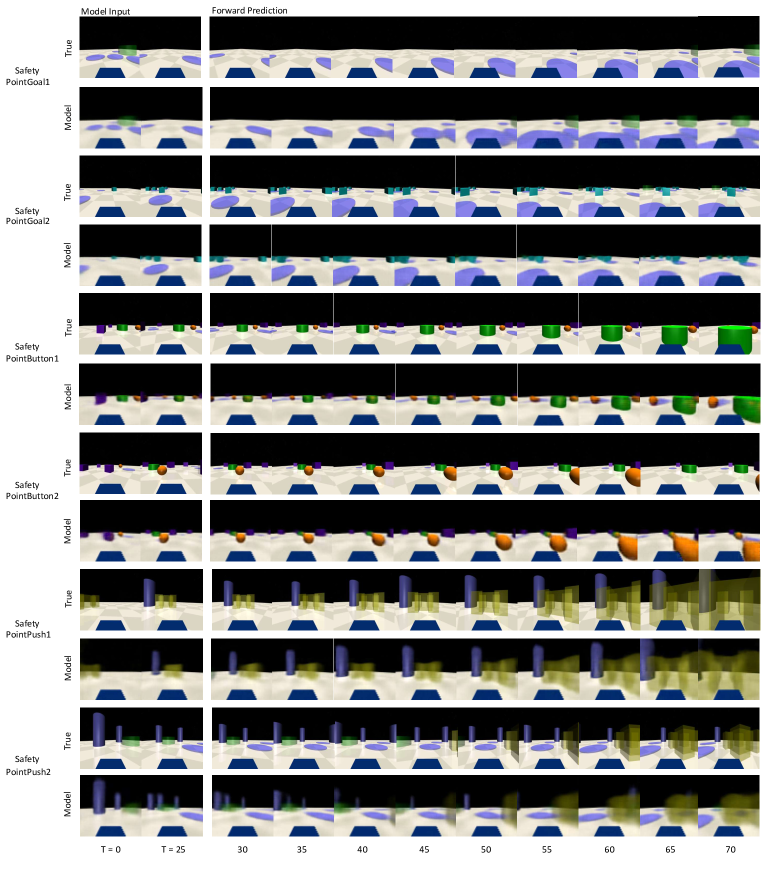
Figure 8: The video predictions in the tasks of the Point agent. In SafetyPointGoal1, the model leverages observed goals to forecast subsequent ones in future frames. In SafetyPointGoal2, the oncoming rightward navigational movement of the robot to avoid an obstacle is predicted by the model. In the SafetyPointButton1, the model predicts the robot’s direction toward the green goal. For SafetyPointButton2, the model anticipates the robot’s trajectory, bypassing the yellow sphere on its left. In the SafetyPointPush1, the model foresees the robot’s intention to utilize its head to mobilize the box. Finally, in SafetyPointPush2, the model discerns the emergence of hitherto unseen crates in future frames, indicating the model’s prediction ability of environmental transition dynamics.

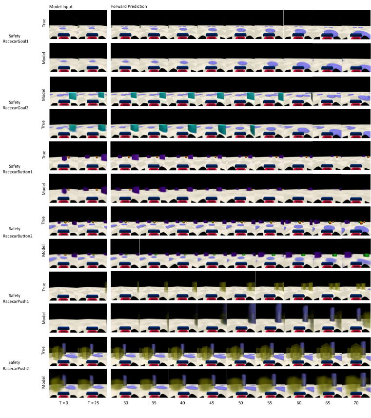
Figure 9: The video predictions of the racecar agent. In SafetyRacecargoal1, the world model anticipates the adjustment of agent direction towards a circular obstacle. Similarly, within the SafetyRacecargoal2, the model predicts the Racecar’s incremental deviation from a vase. In SafetyRacecarButton1, the world model predicts the Racecar’s nuanced navigation to avoid a right-side obstacle. In SafetyRacecarButton2, the model predicts the Racecar’s incremental distance toward a circular obstacle. In SafetyRacecarPush1 and SafetyRacecarPush2 tasks, the model predicts the emergence of the box and predicts the Racecar’s direction towards a box, respectively.

D.2 DreamerV3 vs SafeDreamer

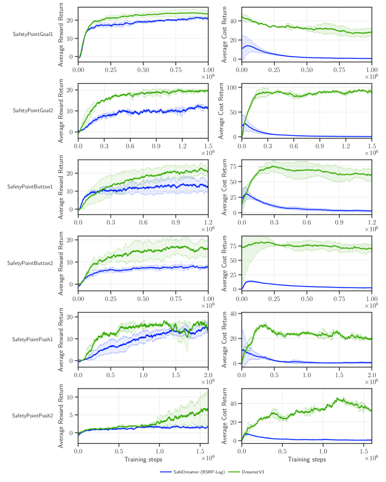
Figure 10: The comparison of SafeDreamer (BSRP-Lag) with DreamerV3 in the task of Point agent.

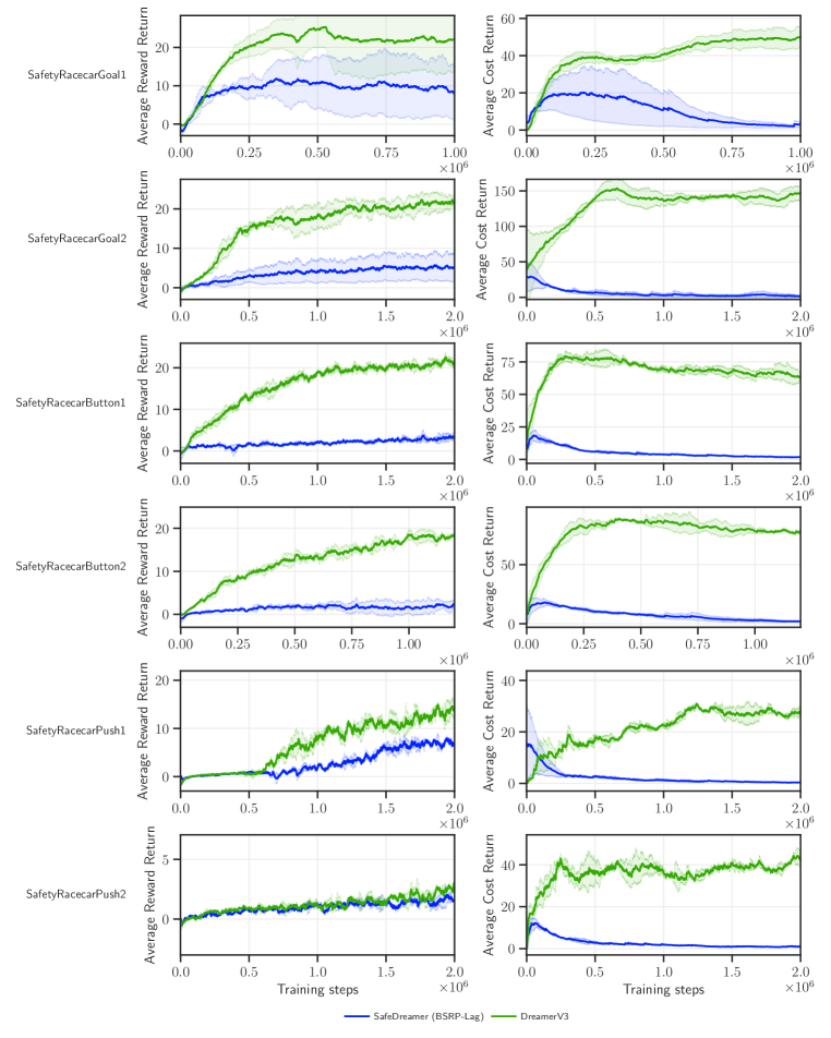
Figure 11: The comparison of SafeDreamer (BSRP-Lag) with DreamerV3 in the task of Racecar.

D.3 The comparison of SafeDreamer with other baseline algorithms.

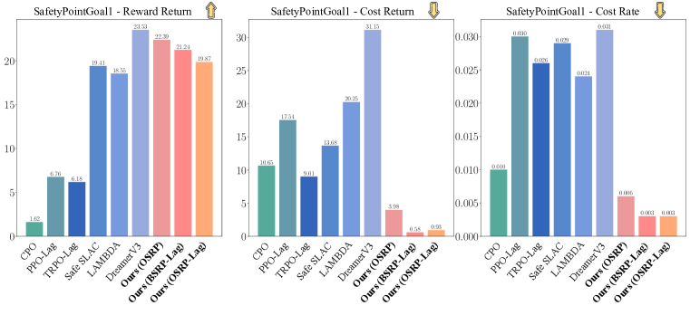
Figure 12: Experimental results in SafetyPointGoal1.

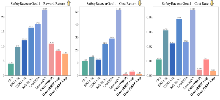
Figure 13: Experimental results in SafetyRacecarGoal1.

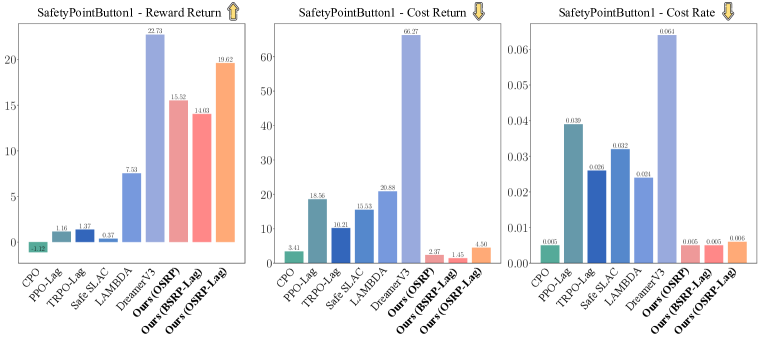
Figure 14: Experimental results in SafetyPointButton1.

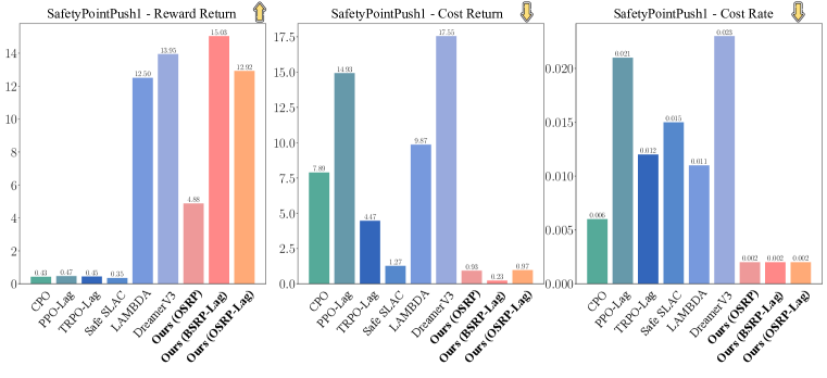
Figure 15: Experimental results in SafetyPointPush1.

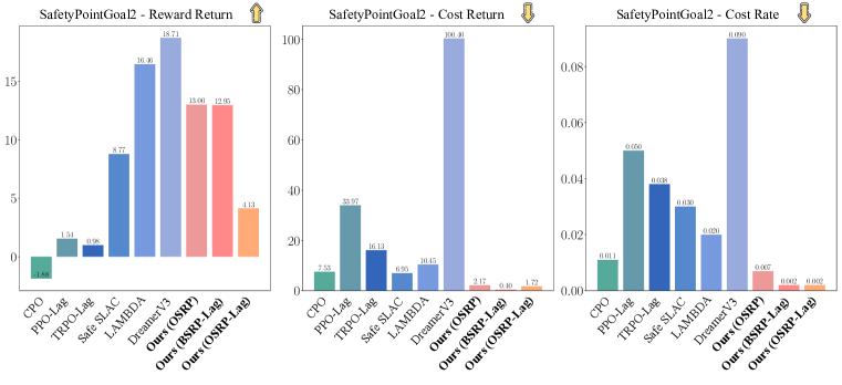
Figure 16: Experimental results in SafetyPointGoal2.

Appendix E Environments

Safety-Gymnasium is an environment library specifically designed for SafeRL. This library builds on the foundational Gymnasium API (Brockman et al., 2016; Foundation, 2022), utilizing the high-performance MuJoCo engine (Todorov et al., 2012). We conducted experiments in five different environments, namely, SafetyPointGoal1, SafetyPointGoal2, SafetyPointPush1, SafetyPointButton1, and SafetyRacecarGoal1, as illustrated in Figure 17.

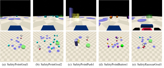
Figure 17: The tasks in Safety-Gymnasium.

E.1 Agent Specification

We consider two robots: Point and Racecar (as shown in Figure 18). To potentially enhance learning with neural networks, we maintain all actions as continuous and linearly scaled to the range of [-1, +1]. Detailed descriptions of the robots are provided as follows:

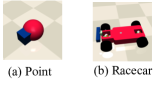
Figure 18: Point and Racecar robots.

Point. The Point robot, functioning in a 2D plane, is controlled by two distinct actuators: one governing rotation and another controlling linear movement. This separation of controls significantly eases its navigation. A small square, positioned in the robot’s front, assists in visually determining its orientation and crucially supports Point in effectively manipulating boxes encountered during tasks.

Racecar. The robot exhibits realistic car dynamics, operating in three dimensions, and controlled by a velocity and a position servo. The former adjusts the rear wheel speed to the target, and the latter fine-tunes the front wheel steering angle. The dynamics model is informed by the widely recognized MIT Racecar project. To achieve the designated goal, it must appropriately coordinate the steering angle and speed, mirroring human car operation.

E.2 Task Representation

Tasks within Safety-Gymnasium are distinct and are confined to a single environment each, as shown in Figure 19.

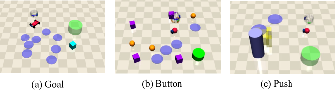
Figure 19: Tasks from Safety-Gymnasium were employed in this paper.

Goal: The task requires a robot to navigate towards multiple target positions. Upon each successful arrival, the robot’s goal position is randomly reset, retaining the global configuration. Attaining a target location, signified by entering the goal circle, provides a sparse reward. Additionally, a dense reward encourages the robot’s progression through proximity to the target.

Push: The task requires a robot to manipulate a box towards several target locations. Like the goal task, a new random target location is generated after each successful completion. The sparse reward is granted when the box enters the designated goal circle. The dense reward comprises two parts: one for narrowing the agent-box distance, and another for advancing the box towards the final target.

Button: The task requires the activation of numerous target buttons distributed across the environment. The agent navigates and interacts with the currently highlighted button, the goal button. Upon pressing the correct button, a new goal button is highlighted, while maintaining the overall environment. The sparse reward is issued upon successfully activating the current goal button, with the dense reward component encouraging progression toward the highlighted target button.

E.3 Constraint Specification

Pillars: These are used to symbolize substantial cylindrical obstacles within the environment, typically incurring costs upon contact.

Hazards: These are integrated to depict risky areas within the environment that induce costs when an agent navigates into them.

Vases: Exclusively incorporated for Goal tasks, vases denote static and delicate objects within the environment. Contact or displacement of these objects yields costs for the agent.

Gremlins: Specifically employed for Button tasks, gremlins signify dynamic objects within the environment that can engage with the agent. Contact with these objects yields costs for the agent.

E.4 Evaluation Metrics

In our experiments, we employed a specific definition of finite horizon undiscounted return and cumulative cost. Furthermore, we unified all safety requirements into a single constraint (Ray et al., 2019). The safety assessment of the algorithm was conducted based on three key metrics: average episodic return, average episodic cost, and the convergence speed of the average episodic cost. These metrics served as the fundamental basis for ranking the agents, and their utilization as comparison criteria has garnered widespread recognition within the SafeRL community (Achiam et al., 2017; Zhang et al., 2020; As et al., 2022).

• Any agent that fails to satisfy the safety constraints is considered inferior to agents that meet these requirements or limitations. In other words, meeting the constraint is a prerequisite for considering an agent superior.

• When comparing two agents, A and B, assuming both agents satisfy the safety constraints and have undergone the same number of interactions with the environment, agent A is deemed superior to agent B if it consistently outperforms agent B in terms of return. Simply put, if agent A consistently achieves higher rewards over time, it is considered superior to agent B.

• In scenarios where both agents satisfy the safety constraint and report similar rewards, their relative superiority is determined by comparing the convergence speed of the average episodic cost. This metric signifies the rate at which the policy can transition from an initially unsafe policy to a feasible set. The importance of this metric in safe RL research cannot be overstated.

References

- Achiam et al. (2017) Joshua Achiam, David Held, Aviv Tamar, and Pieter Abbeel. Constrained policy optimization. In International conference on machine learning, pp. 22–31. PMLR, 2017.
- Altman (1999) Eitan Altman. Constrained Markov decision processes: stochastic modeling. Routledge, 1999.
- As et al. (2022) Yarden As, Ilnura Usmanova, Sebastian Curi, and Andreas Krause. Constrained policy optimization via bayesian world models. arXiv preprint arXiv:2201.09802, 2022.
- Bellemare et al. (2017) Marc G Bellemare, Will Dabney, and Rémi Munos. A distributional perspective on reinforcement learning. In International conference on machine learning, pp. 449–458. PMLR, 2017.
- Boyd & Vandenberghe (2004) Stephen P Boyd and Lieven Vandenberghe. Convex optimization. Cambridge university press, 2004.
- Brockman et al. (2016) Greg Brockman, Vicki Cheung, Ludwig Pettersson, Jonas Schneider, John Schulman, Jie Tang, and Wojciech Zaremba. Openai gym. arXiv preprint arXiv:1606.01540, 2016.
- Camacho et al. (2007) Eduardo F Camacho, Carlos Bordons, Eduardo F Camacho, and Carlos Bordons. Model predictive controllers. Springer, 2007.
- Chen et al. (2022) Yuanpei Chen, Tianhao Wu, Shengjie Wang, Xidong Feng, Jiechuan Jiang, Zongqing Lu, Stephen McAleer, Hao Dong, Song-Chun Zhu, and Yaodong Yang. Towards human-level bimanual dexterous manipulation with reinforcement learning. Advances in Neural Information Processing Systems, 35:5150–5163, 2022.
- Cho et al. (2014) Kyunghyun Cho, Bart Van Merriënboer, Caglar Gulcehre, Dzmitry Bahdanau, Fethi Bougares, Holger Schwenk, and Yoshua Bengio. Learning phrase representations using rnn encoder-decoder for statistical machine translation. arXiv preprint arXiv:1406.1078, 2014.
- Dai et al. (2023) Juntao Dai, Jiaming Ji, Long Yang, Qian Zheng, and Gang Pan. Augmented proximal policy optimization for safe reinforcement learning. In Proceedings of the AAAI Conference on Artificial Intelligence, volume 37, pp. 7288–7295, 2023.
- Feng et al. (2023) Shuo Feng, Haowei Sun, Xintao Yan, Haojie Zhu, Zhengxia Zou, Shengyin Shen, and Henry X Liu. Dense reinforcement learning for safety validation of autonomous vehicles. Nature, 615(7953):620–627, 2023.
- Foundation (2022) Farama Foundation. A standard api for single-agent reinforcement learning environments, with popular reference environments and related utilities (formerly gym). https://github.com/Farama-Foundation/Gymnasium, 2022.
- Garcıa & Fernández (2015) Javier Garcıa and Fernando Fernández. A comprehensive survey on safe reinforcement learning. Journal of Machine Learning Research, 16(1):1437–1480, 2015.
- Haarnoja et al. (2018) Tuomas Haarnoja, Aurick Zhou, Pieter Abbeel, and Sergey Levine. Soft actor-critic: Off-policy maximum entropy deep reinforcement learning with a stochastic actor. In International conference on machine learning, pp. 1861–1870. PMLR, 2018.
- Hafner et al. (2019a) Danijar Hafner, Timothy Lillicrap, Jimmy Ba, and Mohammad Norouzi. Dream to control: Learning behaviors by latent imagination. arXiv preprint arXiv:1912.01603, 2019a.
- Hafner et al. (2019b) Danijar Hafner, Timothy Lillicrap, Ian Fischer, Ruben Villegas, David Ha, Honglak Lee, and James Davidson. Learning latent dynamics for planning from pixels. In International conference on machine learning, pp. 2555–2565. PMLR, 2019b.
- Hafner et al. (2020) Danijar Hafner, Timothy Lillicrap, Mohammad Norouzi, and Jimmy Ba. Mastering atari with discrete world models. arXiv preprint arXiv:2010.02193, 2020.
- Hafner et al. (2023) Danijar Hafner, Jurgis Pasukonis, Jimmy Ba, and Timothy Lillicrap. Mastering diverse domains through world models. arXiv preprint arXiv:2301.04104, 2023.
- Hansen et al. (2022) Nicklas Hansen, Xiaolong Wang, and Hao Su. Temporal difference learning for model predictive control. arXiv preprint arXiv:2203.04955, 2022.
- Hogewind et al. (2022) Yannick Hogewind, Thiago D Simao, Tal Kachman, and Nils Jansen. Safe reinforcement learning from pixels using a stochastic latent representation. arXiv preprint arXiv:2210.01801, 2022.
- Jayant & Bhatnagar (2022) Ashish K Jayant and Shalabh Bhatnagar. Model-based safe deep reinforcement learning via a constrained proximal policy optimization algorithm. Advances in Neural Information Processing Systems, 35:24432–24445, 2022.
- Ji et al. (2023) Jiaming Ji, Borong Zhang, Xuehai Pan, Jiayi Zhou, Weidong Huang, Juntao Dai, and Yaodong Yang. Safety-gymnasium: A unified safe reinforcement learning benchmark, 2023. URL https://github.com/PKU-Alignment/safety-gymnasium.
- Kingma & Welling (2013) Diederik P Kingma and Max Welling. Auto-encoding variational bayes. arXiv preprint arXiv:1312.6114, 2013.
- Koller et al. (2018) Torsten Koller, Felix Berkenkamp, Matteo Turchetta, and Andreas Krause. Learning-based model predictive control for safe exploration. In 2018 IEEE Conference on Decision and Control (CDC), pp. 6059–6066. IEEE, 2018.
- LeCun (2022) Yann LeCun. A path towards autonomous machine intelligence version 0.9. 2, 2022-06-27. Open Review, 62, 2022.
- Lee et al. (2020) Alex X Lee, Anusha Nagabandi, Pieter Abbeel, and Sergey Levine. Stochastic latent actor-critic: Deep reinforcement learning with a latent variable model. Advances in Neural Information Processing Systems, 33:741–752, 2020.
- Li et al. (2022) Quanyi Li, Zhenghao Peng, Lan Feng, Qihang Zhang, Zhenghai Xue, and Bolei Zhou. Metadrive: Composing diverse driving scenarios for generalizable reinforcement learning. IEEE transactions on pattern analysis and machine intelligence, 45(3):3461–3475, 2022.
- Liu et al. (2020) Zuxin Liu, Hongyi Zhou, Baiming Chen, Sicheng Zhong, Martial Hebert, and Ding Zhao. Constrained model-based reinforcement learning with robust cross-entropy method. arXiv preprint arXiv:2010.07968, 2020.
- Moerland et al. (2023) Thomas M Moerland, Joost Broekens, Aske Plaat, Catholijn M Jonker, et al. Model-based reinforcement learning: A survey. Foundations and Trends® in Machine Learning, 16(1):1–118, 2023.
- Nocedal & Wright (2006) Jorge Nocedal and Stephen J. Wright. Numerical Optimization. Springer, New York, NY, USA, second edition, 2006.
- Polydoros & Nalpantidis (2017) Athanasios S Polydoros and Lazaros Nalpantidis. Survey of model-based reinforcement learning: Applications on robotics. Journal of Intelligent & Robotic Systems, 86(2):153–173, 2017.
- Ray et al. (2019) Alex Ray, Joshua Achiam, and Dario Amodei. Benchmarking safe exploration in deep reinforcement learning. arXiv preprint arXiv:1910.01708, 7:1, 2019.
- Schrittwieser et al. (2020) Julian Schrittwieser, Ioannis Antonoglou, Thomas Hubert, Karen Simonyan, Laurent Sifre, Simon Schmitt, Arthur Guez, Edward Lockhart, Demis Hassabis, Thore Graepel, et al. Mastering atari, go, chess and shogi by planning with a learned model. Nature, 588(7839):604–609, 2020.
- Schulman et al. (2017) John Schulman, Filip Wolski, Prafulla Dhariwal, Alec Radford, and Oleg Klimov. Proximal policy optimization algorithms. arXiv preprint arXiv:1707.06347, 2017.
- Sikchi et al. (2022) Harshit Sikchi, Wenxuan Zhou, and David Held. Learning off-policy with online planning. In Conference on Robot Learning, pp. 1622–1633. PMLR, 2022.
- Simo & Laursen (1992) J Ci Simo and TA1143885 Laursen. An augmented lagrangian treatment of contact problems involving friction. Computers & Structures, 42(1):97–116, 1992.
- Stooke et al. (2020) Adam Stooke, Joshua Achiam, and Pieter Abbeel. Responsive safety in reinforcement learning by pid lagrangian methods. In International Conference on Machine Learning, pp. 9133–9143. PMLR, 2020.
- Sutton & Barto (2018) Richard S Sutton and Andrew G Barto. Reinforcement learning: An introduction. MIT press, 2018.
- Thomas et al. (2021) Garrett Thomas, Yuping Luo, and Tengyu Ma. Safe reinforcement learning by imagining the near future. Advances in Neural Information Processing Systems, 34:13859–13869, 2021.
- Todorov et al. (2012) Emanuel Todorov, Tom Erez, and Yuval Tassa. Mujoco: A physics engine for model-based control. In 2012 IEEE/RSJ international conference on intelligent robots and systems, pp. 5026–5033. IEEE, 2012.
- Wabersich & Zeilinger (2021) Kim P. Wabersich and Melanie N. Zeilinger. A predictive safety filter for learning-based control of constrained nonlinear dynamical systems, 2021.
- Webber (2012) J Beau W Webber. A bi-symmetric log transformation for wide-range data. Measurement Science and Technology, 24(2):027001, 2012.
- Wen & Topcu (2018) Min Wen and Ufuk Topcu. Constrained cross-entropy method for safe reinforcement learning. Advances in Neural Information Processing Systems, 31, 2018.
- Yang et al. (2022) Long Yang, Jiaming Ji, Juntao Dai, Linrui Zhang, Binbin Zhou, Pengfei Li, Yaodong Yang, and Gang Pan. Constrained update projection approach to safe policy optimization. arXiv preprint arXiv:2209.07089, 2022.
- Yang et al. (2020) Tsung-Yen Yang, Justinian Rosca, Karthik Narasimhan, and Peter J Ramadge. Projection-based constrained policy optimization. arXiv preprint arXiv:2010.03152, 2020.
- Zhang et al. (2020) Yiming Zhang, Quan Vuong, and Keith Ross. First order constrained optimization in policy space. Advances in Neural Information Processing Systems, 33:15338–15349, 2020.