The Burke-Gaffney Observatory: A fully roboticized remote-access observatory with a low resolution spectrograph

Abstract

We describe the current state of the Burke-Gaffney Observatory (BGO) at Saint Mary’s University - a unique fully roboticized remote-access observatory that allows students to carry out imaging, photometry, and spectroscopy projects remotely from anywhere in the world via a web browser or social media. Stellar spectroscopy is available with the ALPY 600 low resolution grism spectrograph equipped with a CCD detector. We describe our custom CCD spectroscopy reduction procedure written in the Python programming language and demonstrate the quality of fits of synthetic spectra computed with the ChromaStarServer (CSS) code to BGO spectra. The facility along with the accompanying Python BGO spectroscopy reduction package and the CSS spectrum synthesis code provide an accessible means for students anywhere to carry our projects at the undergraduate honours level. BGO web pages for potential observers are at the site: observatory.smu.ca/bgo-useme. All codes are available from the OpenStars www site: openstars.smu.ca/

1 Introduction

The Burke-Gaffney Observatory (BGO, lat. $+44\,37\,50$, long. $-63\,34\,52$) at Saint Mary’s University (SMU) underwent a significant refurbishment in 2013 and now consists of a 0.6 m (24”) $f/6.5$ Planewave telescope (model CDK24) with a corrected Dall-Kirkham optical configuration. It is equipped with an $f/4$ model PF0035 ALPY 600 grism spectrograph from Shelyak Instruments. This optical combination involves an inexpensive lightweight spectrograph of low $f$ value paired with a telescope of larger $f$ value and is a compromise between optical matching and affordability. We operate the spectrograph with a slit width of 23 $\mu$m corresponding to a spectral resolving power, $R$, of $\sim 600$, equivalent to a spectral resolution element of $\Delta v\sim 500$ km s^-1 at $\lambda\sim 6000$ Å. The camera is a model Atik 314L+ equipped with a Sony ICX 205AL sensor CCD with $1391\times 1039$ imaging pixels of size $6.45\times 6.45$ $\mu$m. The setup provides a reciprocal linear dispersion, ${\Delta\lambda/\Delta x}$, of $\sim 420$ Å  mm^-1 and a spectral range, $\Delta\lambda$, of $\sim 3750$ Å, effectively covering the entire visible band from $\sim 4000$ to $\sim 7000$ Å  after accounting for edge effects.

The BGO is a fully automatic, roboticized facility, and imaging and photometric observing requests are handled in queued observing mode. The acquisition of spectra is a much more complex process than direct imaging, and approved observers submit a request for a synchronous observing session via email or by social media and carry out a session remotely via a web browser and the BGO observing portal. This process requires low-level access to multiple software applications to control the telescope, CCD camera, calibration light sources, and to position targets precisely at the spectrograph slit. Manual guiding is often required when the target is faint.

The BGO observing portal provides the following functions: 1) Telescope pointing via the Earth-Centred-Universe (ECU) telescope control and planetarium application and accompanying automatic dome rotation via the custom dome connection software; 2) A large object database via ECU; 3) A continuously updated view from the spectrograph guide camera for slit monitoring; 4) Acquisition and immediate display of snapshots of the field of view and of the spectrum for preliminary inspection; 5) Science exposures of the spectrum.

Our experience is that for bright stars ($V<7$) the diurnal tracking is very stable and that once the star is manually centered on the slit the pointing does not require manual correction. The ”seeing” at the BGO site is significant ($>1^{\prime\prime}$) and much of the light falls outside the slit. Advantages are that for bright stars this provides more uniform illumination across the slit and a significant distribution of light in the cross-dispersion direction.

Fig. 1 shows a screen shot of the BGO observing portal during a spectroscopy session on 22 June 2023 by the author with the program star HR5616 ($\psi$ Boo, K2 III, $V=4.54$ (Hoffleit & Warren, 1991)), including the ECU planetarium and telescope control panel and the live monitoring view from the spectrograph slit-plane guide camera. Fig. 2 shows an enlarged version of the view from the spectrograph guide camera and Fig. 3 shows a 20 s snapshot of the spectral image taken with the Atik 314L+ science camera. Potential observers, especially students at all levels, are encouraged to visit the BGO Robotic Telescope page at observatory.smu.ca/bgo-useme to learn how to become an approved observer and for a primer on interacting with the BGO remotely.

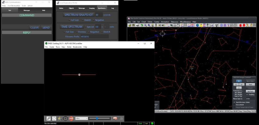
Figure 1: HR 5616: Screenshot of the robotic BGO observing portal during a spectroscopy session including the ECU planetarium and telescope control interface, and the view from the spectrograph guide camera.

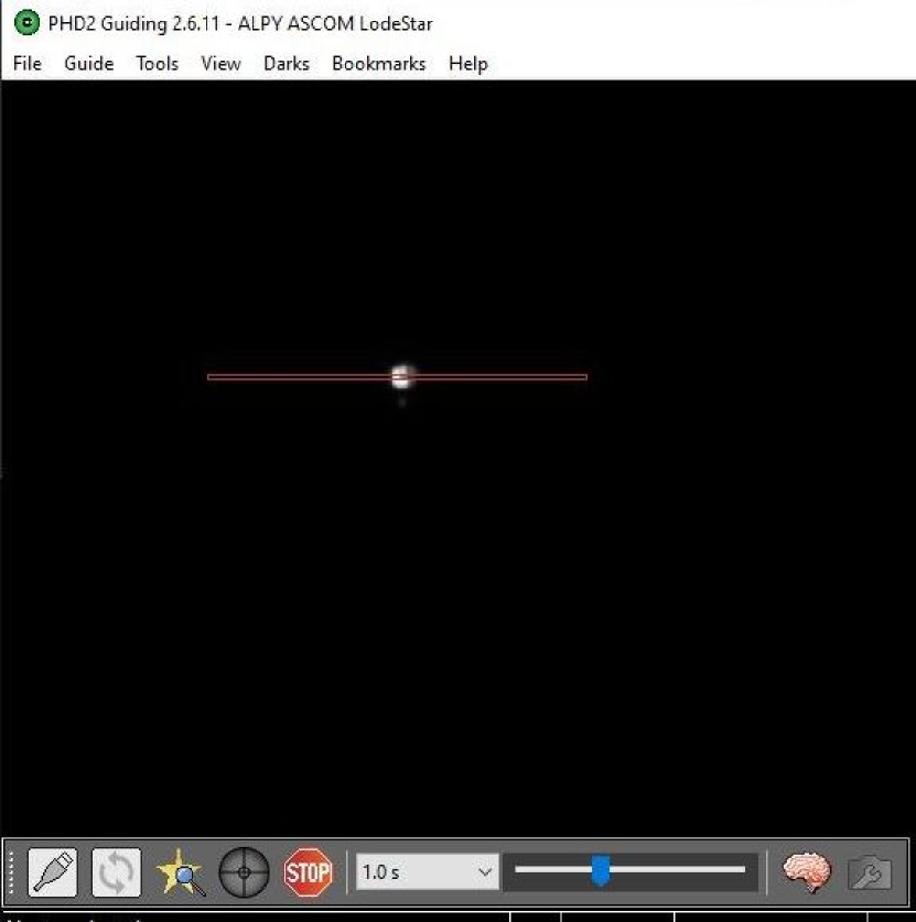
Figure 2: The same as Fig. 1, but showing only the view from the spectrograph guide camera. The red rectangle is the projection of the 23 $\mu$m slit onto the sky.

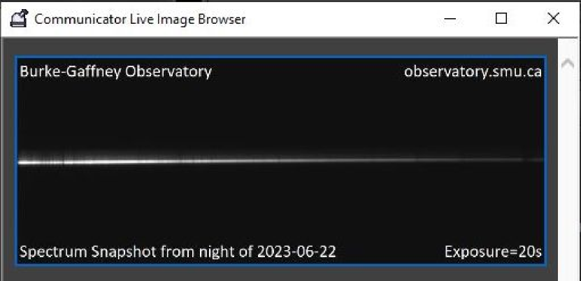
Figure 3: Same as Fig. 1, but showing only a 20 s ”snapshot” of the spectral image taken with the ALPY 600 spectrograph and the Atik 314L+ imaging camera and Sony ICX 205AL CCD.

2 Observations

Table 1 and Fig. 4 present a set of commissioning spectra of seven bright stars acquired on 15 April 2021 by one of the co-authors who was the BGO Director and Astronomy Technician at the time (Lane). The set includes six luminosity class V stars spanning the range of spectral class from K5 to B4 and one luminosity class III star of spectral class M3.

Table 1: Commissioning stars observed in April 2021 with the ALPY 600 spectrograph. All stellar data are those of Hoffleit & Warren (1991)

Designation	$V$	$B-V$	Sp. Type	Exp. time (s)
HR3521	6.23	+1.62	M3 III	60
HR3580	6.44	-	K5 III	120
HR3309	6.32	+0.62	G5 V	120
HR4455	5.77	+0.46	F5 V	120
HR3333	5.95	+0.19	A5 V	60
HR3348	6.18	-0.03	A0 V	60
HR4456	5.95	-0.16	B4 V	120

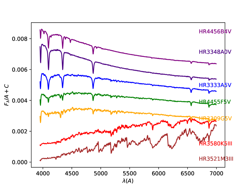
Figure 4: Set of seven commissioning spectra for the seven stars listed in Tab. 1 for the ALPY 600 spectrograph at the BGO.

3 Reduction procedure

To gain experience with the instrument, and to establish a local reduction procedure that SMU students can modify, we have chosen to develop an independent procedure in the Python programming language. In what follows we take CCD pixel columns (fixed $x$-coordinate) to run in the cross-dispersion direction, and CCD pixel rows (fixed $y$-coordinate) to run along the dispersion axis. Therefore $x$ ranges from 1 to 1391 and $y$ ranges from 1 to 1039.

1) $\lambda$-calibration: We identify nine spectral lines of known wavelength, $\lambda_{\rm n}$ ($n=0,1,...8$), in the emission spectrum of an Ar-Ne lamp, measure their centroid pixel column positions, $x_{\rm n}$, and determine the best fitting coefficients, $a_{\rm m}$ ($m=0,1,2)$, of a $2^{\rm nd}$ order polynomial for the measured $\lambda_{\rm n}(x_{\rm n})$ relation using the numpy (Harris et al., 2020) polyfit() procedure. We then generate a $1D$ $\lambda$ array of length $1391$ elements, $x$, with the expression

$$\lambda(x)=a_{2}x^{2}+a_{1}x+a_{0}$$ (1)

2) Background subtraction: The software package supplied with the ALPY 600 spectrograph includes a post-processing pipeline that automatically applies flat-field division, and bias- and dark-current-subtraction corrections. We extract the value of the ’pedestal” that is added by the analog-to-digital (ADU) conversion from the FITS header and subtract its value from each pixel. We have found that this procedure yields images in which there is still an approximately flat background of $\leq 10$ counts per pixel across the chip in addition to the spectral image, which we infer includes scattered light. We fit a $2D$ function corresponding to a $0^{\rm th}$ order polynomial in both the pixel column, $x$, and pixel row, $y$, dimensions (ie. a flat background) to two rectangular samples regions on either side of the spectral image and away from the edges of the chip consisting of $1371$ columns ($10<x<1381$) and $40$ rows (($10<y<50$) and ($989<y<1029$)) by finding the average residual count per pixel among the two sample regions, and then subtract the average from every pixel. This yields a spectral image with a residual count of $\sim 0$ counts per pixel.

3) Spectrum location: The position of the spectral image on the chip, as indicated by the approximate row ($y$ value) where the cross-dispersion profile is brightest, depends on the distribution of the stellar point-spread-function (PSF) along the slit, and varies significantly from exposure to exposure. We automatically locate the row of maximum counts, $y^{\rm max}_{\rm n}(x_{\rm n})$, in three representative columns of $x_{\rm n}$ value of 100, 695 (mid-chip) and 1291 and fit a $1^{\rm st}$ order polynomial to the $y^{\rm max}_{\rm n}(x_{\rm n})$ relation to trace the contour of greatest brightness across the chip. We find that the dispersion axis is tilted by $\sim 0.5^{\rm o}$ with respect to the CCD rows, corresponding to a $\Delta y$ value of $\sim 12$ rows over the $1391$ columns.

4) Model cross-dispersion weight profile: We form a $1D$ normalized smooth cross-dispersion weight profile by computing row-wise average counts over the middle 20 columns ($x=686$ to $706$) on the chip, taking the square root, and dividing each of the 20 elements in the profile by the square root of the maximum number of counts among the included pixels. We truncate the wings of the profile at row ($y$) values of the centroid $y$ value $\pm 15$, so that the $1D$ profile has 30 elements. Fig. 5 shows the average observed cross dispersion profile and the derived weight profile, arbitrarily re-scaled for visibility, for the case of our observation of HR 3580 (K5 III).

5) Spectrum formation: We form a $1D$ spectrum by summing the counts in rows ($y$ values) within the range of $\pm 15$ of the row where the cross-dispersion profile is brightest in each column ($x$ value), weighted by our model cross-dispersion profile (see Step 4)). This root-weighting gives higher weight to pixels near the centre of the cross-dispersion profile that have higher signal-to-noise ($S/N$) while still taking advantage of the signal in the cross-dispersion wings.

6) Continuum rectification: Rectification of broadband high $\Delta\lambda/\Delta x$ spectra of late-type stars is challenging because there are no regions that can be obviously identified as continuum regions. Our goal is to develop a procedure that automatically normalizes the spectrum over most of the visible band for spectral classes $B$ to $K$, for which the spectrum is not too affected by deep broad TiO bands or by emission lines. Normalizing the spectrum takes place in three steps:

a) Instrumental response: An initial very approximate correction is made by dividing the spectrum by a smooth instrumental response function that was provided by the BGO staff. This correction greatly reduces the slope of the spectrum along the dispersion axis. Then a $0^{\rm th}$ order normalization is made by dividing every element by the maximum value of this quotient spectrum.

b) Fit to truncated mean binned counts: We avoid edge effects in our continuum fitting by omitting a chosen number of columns at both ends of the spectrum. We form mean binned counts by choosing a number of bins and assigning the mean number of counts in each bin, $f^{1}_{\rm n}$ to the central pixel ($x_{\rm n}$-value) of that bin. We then fit a polynomial to the $f^{1}_{\rm n}(x_{\rm n})$ relation with the numpy.polyfit() procedure, use the best-fit coefficients to generate the corresponding normalizing function $f^{1}(x)$ and divide the spectrum from Step 6 a) element-wise by $f^{1}(x)$.

c) Fit to truncated maximum binned counts: For late-type stars, Step 6 b) can produce a spectrum with peak counts significantly greater than unity in local regions throughout the spectrum. We then follow a similar truncation and binning procedure as Step 6 b) except we fit a second polynomial, $f^{2}_{\rm n}(x_{\rm n})$ to the maximum number of counts among the pixels in each bin, $f^{2}_{\rm n}$, and divide the spectrum from Step 6 b) by the corresponding normalizing function $f^{2}(x)$.

Our experience is that we can reliably produce automatically approximately continuum-rectified spectra over much of the central region of the spectrum for a wide range of spectral classes, including class $K$, by choosing 13 bins for Step 6 b), corresponding to $\sim 200$ Å  per bin, and fitting with a $5^{\rm th}$ order polynomial, and 13 bins for Step 6 c) and a $5^{\rm th}$ order polynomial. We find we can achieve reasonable normalization in a spectral region truncated to the range $\lambda$4300 to 6800 Å. Figs. 6 and 7 show the binned counts, fitting function, and partially re-normalized spectrum for Steps 6 b) and c) for the case of a B4 V star (HR4456) and Figs. 8 and 9 show the same for the more challenging case of a K5 III star (HR3580).

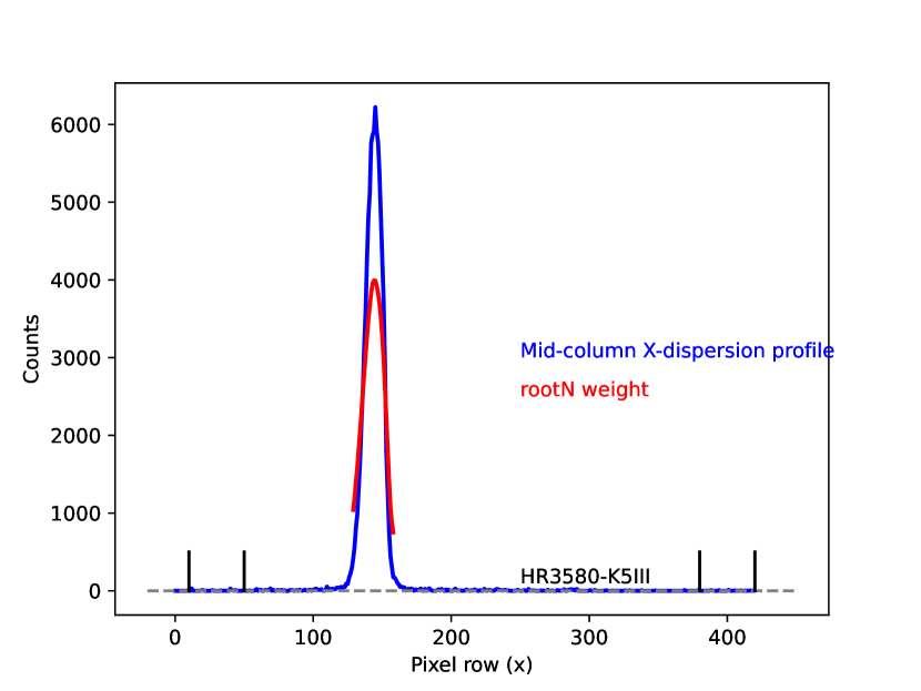
Figure 5: Observed cross dispersion profile averaged over 20 columns at chip center ($x=686$ to $706$, blue line) and the derived root-N weight profile that was used to weight the rows ($y$ values) when extracting the 1$D$ spectrum (Step 4, red line). The weight profile peaks at a value of $\sim 1$ and has been arbitrarily re-scaled for visibility. Also shown are the row ($y$-value) ranges of the regions used to fit the $0^{\rm th}$ order background signal (Step 2).

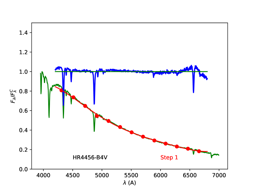
Figure 6: Step b) of our general procedure for automatic continuum rectification of broadband spectra (Step 6) for B4 V star HR 4456. Green line: BGO ALPY 600 spectrum after division by an instrumental response function and a $0^{\rm th}$-order normalization to unity, $F^{0}(x)$; Red points: Mean binned counts; Red line: Polynomial fit to mean counts points, $f^{1}(x)$; Blue line: Spectrum with refined normalization, $F^{1}(x)=F^{0}(x)/f^{1}(x)$. Horizontal straight line: $F(x)$ of unity for reference.

Figure 7: Step c) of our general procedure for automatic continuum rectification of broadband spectra for the star of Fig. 6. Blue line: Output from Step b), $F^{1}(x)$ (see Fig. 6); Red points: Maximum binned counts; Red line: Polynomial fit to maximum counts points, $f^{2}(x)$; Black line: Spectrum with final normalization, $F^{2}(x)=F^{1}(x)/f^{2}(x)$. Horizontal straight line: $F(x)$ of unity for reference.

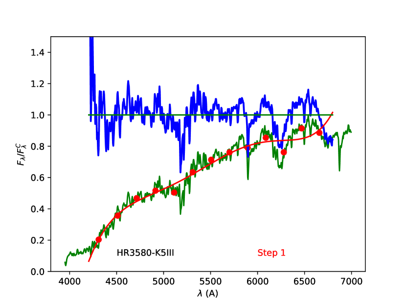
Figure 8: Same as Fig. 6, except for the K5 III star HR 3580.

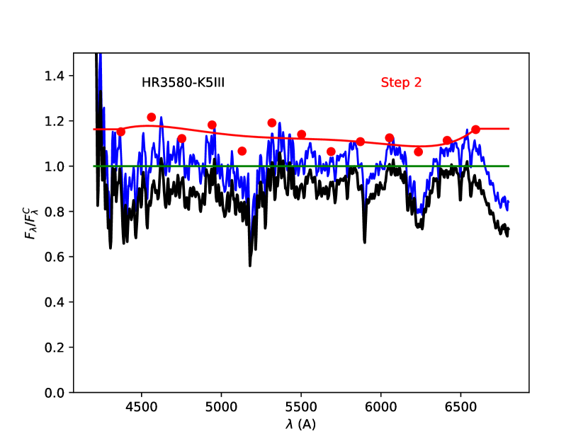
Figure 9: Same as Fig. 7, except for the K5 III star HR 3580.

4 Comparison of BGO and model spectra

In a companion paper we describe a grid of stellar atmospheric models computed with the ChromaStarServer (CSS) code that spans the $T_{\rm eff}$ range 3600 to 22  000 K with $\log g=4.5$ and $[{{\rm A}\over{\rm H}}]=0.0$, with $\Delta T_{\rm eff}$ intervals of 200 K for $T_{\rm eff}\leq 8000$ K and 400 K for $T_{\rm eff}>8000$ K along with models of $\log g=2.0$ at select $T_{\rm eff}$ values less than 5000 K and the corresponding CSS synthetic spectra in the $\lambda$ range 400 to 750 nm. In Figs. 10, 11, and 12 we show the comparison between observed spectra from our BGO observing run and synthetic spectra from our model grid bracketing the nominal $T_{\rm eff}$ value corresponding to the spectra type listed in Hoffleit & Warren (1991). Nominal $T_{\rm eff}$ values were taken from Appendix G of Carroll & Ostlie (2007). Because we can only achieve an approximate continuum rectification for late type stars with high $\Delta\lambda/\Delta x$ broadband data, we do not attempt a quantitative fit based on minimizing a fitting statistic, but only a perform a visual inspection of the fit quality.

As discussed in the companion paper, at the low $R$ and high ${{\Delta\lambda}\over{\Delta x}}$ values of these spectra, the main features at which we can assess the fit within the $\sim 4200$ to $\sim 6800$ Å  rectification range for GK stars are the Na I $D_{\rm 2}$ doublet at $\lambda 5900$ Å  and the TiO C${}_{\rm 3}\Delta$-X${}_{\rm 3}\Delta$ ($\alpha$ system, $\lambda_{\rm 00}~{}5170$ Å) and the B${}_{\rm 3}\Pi$-X${}_{\rm 3}\Delta$ ($\gamma$’ system, $\lambda_{\rm 00}~{}6193$ Å) bands. For A and B stars, at our $R$ and ${{\Delta\lambda}\over{\Delta x}}$ values, the main features at which we can judge the fit within the rectification range are the H I $\beta$ and $\gamma$ lines. This is sufficient to allow students to do projects at the undergraduate honours level in which they carry out and reduce their own BGO spectroscopy to coarsely classify stars to within a few spectral subclasses accuracy. In the process, they will gain valuable experience with the procedures of observational and computational stellar spectroscopy within a Python IDE running on commonplace Windows or Linux computer.

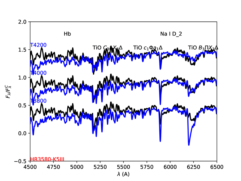
Figure 10: HR3580 (K5 III): Black: Observed spectrum from our BGO program plotted with three different vertical offsets. Blue: Synthetic spectra for models of $\log g=2.0$, $[{{\rm A}\over{\rm H}}]=0.0$, and $T_{\rm eff}$ values of 3800, 4000, and 4200 K in order of increasing vertical offset.

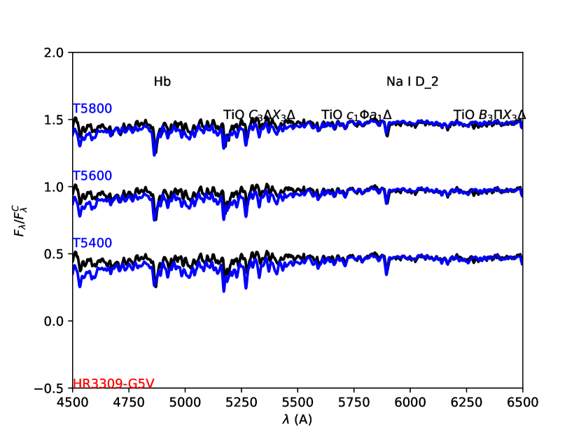
Figure 11: Same as Fig. 10 except for star HR3309 (G5 V) and models of $T_{\rm eff}$ values of 5400, 5600, and 5800 K.

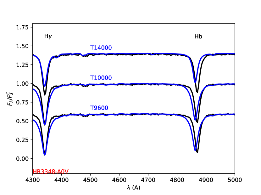
Figure 12: Same as Fig. 10 except for star HR3348 (A0 V) and models of $T_{\rm eff}$ values of 9600, 10000, and 14  000 K.

References

- Carroll & Ostlie (2007) Carroll, B.W. & Ostlie, D.A., 2007, An Introduction to Modern Astrophysics, 2nd Ed., Pearson - Addison Wesley (San Francisco)
- Grevesse & Sauval (1998) Grevesse, N., Sauval, A.J., 1998, Space Science Reviews, 85, 161
- Harris et al. (2020) Harris, C.R., Millman, K.J., van der Walt, S.J. et al., 2020, Nature, 585, 357
- Hoffleit & Warren (1991) Hoffleit, D. & Warren, Jr W.H., 1991, The Bright Star Catalogue, 5th Rev. Ed.
- Kramida et al. (2015) Kramida, A., Ralchenko, Yu., Reader, J., and NIST ASD Team (2015). NIST Atomic Spectra Database (ver. 5.3), [Online]. Available: http://physics.nist.gov/asd [2015, November 26]. National Institute of Standards and Technology, Gaithersburg, MD.
- Pakhomov, Ryabchikova & Piskunov (2019) Pakhomov, Yu. V., Ryabchikova, T.A. & Piskunov, N.E., 2019, Astronomy Reports, 63, 1010
- Peterson, Dalle Ore & Kurucz (1993) Peterson, R.C., Dalle Ore, C.M., Kurucz, R.L., 1993, ApJ, 404, 333
- Ryabchikova et al. (2015) Ryabchikova, T., Piskunov, N., Kurucz, R. L., Stempels, H. C., Heiter, U., Pakhomov, Yu, Barklem, P. S., 2015, Physica Scripta, 90, 054005
- Short (2016) Short, C.I., 2016, PASP, 128, 104503
- Short & Bennett (2021) Short, C.I. & Bennett, P.D., 2021, PASP, 133, 064501