Nowcasting Temporal Trends Using Indirect Surveys
Abstract
Indirect surveys, in which respondents provide information about other people they know, have been proposed for estimating (nowcasting) the size of a hidden population where privacy is important or the hidden population is hard to reach. Examples include estimating casualties in an earthquake, conditions among female sex workers, and the prevalence of drug use and infectious diseases. The Network Scale-up Method (NSUM) is the classical approach to developing estimates from indirect surveys, but it was designed for one-shot surveys. Further, it requires certain assumptions and asking for or estimating the number of individuals in each respondent’s network. In recent years, surveys have been increasingly deployed online and can collect data continuously (e.g., COVID-19 surveys on Facebook during much of the pandemic). Conventional NSUM can be applied to these scenarios by analyzing the data independently at each point in time, but this misses the opportunity of leveraging the temporal dimension. We propose to use the responses from indirect surveys collected over time and develop analytical tools (i) to prove that indirect surveys can provide better estimates for the trends of the hidden population over time, as compared to direct surveys and (ii) to identify appropriate temporal aggregations to improve the estimates. We demonstrate through extensive simulations that our approach outperforms traditional NSUM and direct surveying methods. We also empirically demonstrate the superiority of our approach on a real indirect survey dataset of COVID-19 cases.
1 Introduction
Direct reporting through surveys is the most widely used method for collecting data on a given characteristic among individuals in a population. It is well known that direct surveys sometimes face reliability and efficiency problems, as respondents may refuse to participate or may choose to misreport sensitive private information. An alternative approach to overcome some of these issues is using surveys with indirect reporting, where respondents answer questions about people they know instead of providing information about themselves. These surveys collect what is known in the literature as aggregated relational data (ARD). Their main advantages are primarily two: (1) privacy is preserved as the respondents do not have to report their own status, thus improving participation and data collection about sensitive populations (Rossier 2010); (2) one individual response gives the researchers access to information about many different individuals, thus leading to cost reductions in the data collection (Breza et al. 2020), (Alix-Garcia, Sims, and Costica 2021). Indirect surveys have been employed in a variety of domains, such as estimating the number of casualties in an earthquake (Bernard et al. 1989), conditions among female sex workers (Jing et al. 2018), or the prevalence of drug use (Salganik et al. 2010), HIV (Teo et al. 2019) or COVID-19 (Garcia-Agundez et al. 2021).
While indirect surveys have a long history (Laga, Bao, and Niu 2021), the ubiquity of internet access among the general public has made it possible to develop online indirect surveys, which can be deployed rapidly and allow the continuous collection of ARD, instead of consisting of one-shot surveys. The importance of recurrent online surveys, including indirect surveys, has become apparent during the COVID-19 pandemic, where one of the most important challenges has been estimating (nowcasting) the number of cases (especially when testing was not widely available), the number of deaths, the number of people vaccinated, etc. While the best-known online surveys are the COVID-19 Trends and Impact Surveys (CTIS) (Astley et al. 2021; Salomon et al. 2021), which collected more than 100,000 responses daily, other surveys were also deployed (Geldsetzer 2020; Oliver et al. 2020; Garcia-Agundez et al. 2021).
Our main goals are (i) to quantify the advantages of indirect surveys over direct ones for nowcasting, by determining under what conditions, more accurate estimates can be obtained via indirect questions; and (ii) to develop a new method to identify a hidden temporal trend from the continuously collected ARD from indirect surveys. To achieve these goals, we combine a detailed theoretical analysis with extensive experimental evaluations with both synthetic and real datasets. Given the availability, throughout the paper, we use the COVID-19 surveys dataset as a test case.
1.1 Related Work
ARD from indirect surveys are used to nowcast the size of a subpopulation or hidden population, i.e., the fraction of the population that has some characteristic. For example, in a COVID-19-related survey, a respondent may report on how many people they know who have tested positive recently, and this information will be used to estimate the fraction of the overall population that is infected at that time. Thus, each respondent is expected to provide information about their own personal network (PN) – how many people they know– and the number of people they know who are part of the hidden population (e.g., tested positive).
NSUM
The methods proposed in the literature for the estimation of the size of hidden populations (people infected in our example) using ARD are generally known as Network Scale-Up Methods (NSUM) (Laga, Bao, and Niu 2021). To estimate the size of the hidden population from the ARD, NSUM assumes that the proportion of those belonging to the hidden population within a respondent’s PN is a good approximation to the same proportion in the overall population. NSUM can work well under several assumptions: (1) the respondents can accurately recall the people in their PN, (2) the respondents know, for each person in their PN, if they belong to the hidden population, and (3) all individuals have the same probability of belonging to the hidden population. Errors resulting from violations of these conditions are called recall error, transmission error, and barrier effects, respectively (see (Laga, Bao, and Niu 2021) for more details). Multiple NSUM extensions have been proposed (Laga, Bao, and Niu 2021) but all of them require to request or estimate PN sizes (Killworth et al. 1998b; Laga, Bao, and Niu 2021; Garcia-Agundez et al. 2021), or ask individuals in the hidden population about those who know their condition (Feehan and Salganik 2016).
Our goal is to obtain better estimates of the evolution of the hidden population size without a need to obtain or estimate the size of individuals’ PNs and, thus, without having to rely on the above recall assumptions. Specifically, one of the key contributions of our work is to leverage the temporal dynamics to improve estimates from continuously collected data. We provide analytical tools to unveil the advantages of appropriately aggregating continuous indirect surveys rather than simply using existing methods over fixed temporal windows. To the best of our knowledge, prior work does not leverage the temporal nature of continuous surveys.
1.2 Contributions
We propose a method to estimate the evolution of the size of the hidden population over a period of time using indirect surveys. Our contributions are as follows:
-
•
We propose a latent graph formulation that allows us to prove that the expected response to the indirect survey is proportional to the size of the hidden population (Theorem 1). Unlike existing work, we do not assume that every individual has the same probability of reporting someone belonging to the hidden population.
-
•
We prove that within a reasonable upper bound on the latent graph degree variance, the indirect survey provides a better estimate of the hidden population than the direct survey given the same number of samples (Theorem 2).
- •
-
•
We verify our claims through a simulated generation of the hidden population with a dynamic process and a simulated survey. We present the impact of various survey parameters (Section 3.1).
-
•
We evaluate our approach in the estimation of COVID-19 cases in the US for a period of 18 months (Section 3.2).
Our analytical results can be useful for survey design. Note that our objective is nowcasting (rather than forecasting) the time series of the size of the hidden population.
2 Methodology
2.1 Latent Graph Formulation
Consider a population given by a set . Suppose that, at time , contains a hidden population denoted by , leading to a hidden population rate . Let be a directed graph, where is the set of nodes and is the set of edges. In particular, includes an edge if node possesses knowledge of node and is willing to report whether node belongs to the hidden population. Also, we allow self-loops . These edges may not be the same as those in the contact graph or the social network graph containing the same nodes. The edges present on this (unobserved) graph depend on the specific wording of the survey questions, e.g., “how many in your community …”, “… your household”, “your immediate neighbors and coworkers”, etc.
Consider a random process that selects one node, at time to report the number of its neighbors belonging to the hidden population. We denote by the random variable corresponding to this response. In the surveys, at a given time , multiple nodes are selected randomly (possibly, with replacement) that provide multiple observations for . We will later use the mean and variance of to identify the properties of the sample mean obtained from these responses. Finally, is a random variable representing the in-degree of a randomly selected node, with .
Assumption 1.
For any node belonging to the neighborhood of node , the event is independent of the in-degree of .
This implies that having a certain in-degree does not affect whether a randomly selected neighbor is part of the hidden population. This assumption is more flexible than that used in the traditional NSUM approach, in which every node must have the same probability of finding a neighbor belonging to the hidden population (Laga, Bao, and Niu 2021). Under Assumption 1, nodes can have different probabilities of having neighbors in (for example, this could depend on their respective occupations). However, if we consider the union of neighbors of all nodes with a particular indegree, the probability of a random node in this union belonging to remains , irrespective of the indegree considered. This assumption will allow us to eliminate the need to ask for the in-degree of each node. Based on Assumption 1, we have the following theorem.
Theorem 1.
.
Therefore, the mean indirect response is proportional to what we wish to estimate. Additionally, we make the following observation regarding the underlying graph .
Observation 1.
The mean in-degree of all nodes, , remains constant over time.
This observation is supported by the studies of Dunbar (Dunbar 2010). It can also be observed in the data collected by the Carnegie Mellon University US COVID-19 Trends and Impact Survey (CMU-CTIS) (Salomon et al. 2021), where, over time, different respondents provided the household size in which they reported the number of infections (see Supplementary Material in full version (Srivastava et al. 2023)).
Recall that is not an acquaintance or physical contact network. Instead, the connection of a node in represents the network of people the respondent will think of when answering the question. Respondents may not report on the same people each time the survey is completed. So may be different at each time , but the mean of the in-degrees remains constant. From Observation 1 and Theorem 1, the time series is proportional to time series , representing the fraction of the hidden population, with as the constant of proportionality. Hence, we can estimate the trend of without knowing . For applications in which precise values are needed, if the true value of is available for some then we can estimate and use this constant to estimate at any . For example, when represents the rate of active infections, could correspond to those dates for which serological studies or wastewater concentration data are available.
Comparison Against Direct Reporting.
With direct reporting, each node reports whether it belongs to the hidden population. Thus, for a randomly selected node , the response is the binary indicator function , where iff . Let be a random variable denoting the response of a randomly selected node. Observe that is a binary random variable whose samples follow a Bernoulli distribution with mean and variance . To compare direct and indirect reporting scenarios, we also need to compute the variance of . Since the links in our latent graph do not represent physical contact, neighbors of node are not necessarily dependent, and we introduce a parameter that controls the level of covariance.
Definition 1.
For a pair of nodes and , with a common neighbor u, , for some .
Here implies independence, leads to negative covariance and leads to positive covariance. Now we can find bounds on the variance of .
Lemma 1.
If is the variance of the degree distribution,
| (1) |
Further, .
Suppose we have the same number of responses for and , and , we show that within a practical upper bound of degree variance , the indirect survey is a better estimator than the direct survey.
Lemma 2 (Central Limit Theorem, CLT).
When the number of samples is large, and follow standard normal distribution, where and are the sample means.
Now, we can show, under Lemma 2, that the probability of deviating from the true fraction of hidden population is lower for the estimate obtained from indirect responses compared to direct responses .
Theorem 2.
For any , , if the variance of degree distribution
This means within realistic bounds on degree variance, indirect surveys are better than direct surveys. The condition on is reasonable for applications where at any given time is a small fraction of the population. To see this, first note that if the membership of two neighbors in the hidden population is independent, . Assuming that the maximum degree in the graph is , and , the variance can be bounded using (Bhatia and Davis 2000) by . To satisfy this bound, and still violate the assumption on degree variance in Theorem 2, would require , i.e., for of the population to be in the hidden population (e.g., positive with COVID-19) simultaneously. This is unrealistically high, noting that the highest number of COVID-19 tests performed (which is much higher than reported positive cases) in a week in California was approximately 11.2% ( 20%) of the population. Theorem 2 also motivates framing the indirect survey questions in such a way that the variance of the graph is small.
2.2 Leveraging Smoothness
The hidden population in many real-life processes is driven by smooth dynamic processes, leading to the following.
Observation 2.
and , for some small .
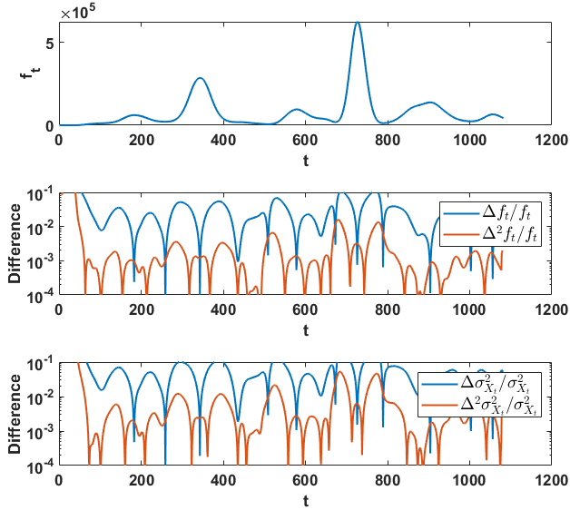
This is reasonable for epidemics as the epidemiology follows smooth dynamics which over a large population should produce smooth case counts. The reported data may appear to be noisy due to reporting behavior, schedule, and delayed dumps (a death occurring today may be reported 1-2 weeks from now). However, the artifacts of reporting to the state dashboards are not something we wish to capture. Instead, we wish to capture the actual incidence of cases based on surveys. An individual will know if their friends are infected independently of how and when it is reported to the state dashboards. To support this observation, we compute from values for COVID-19 reported cases (after denoising and removing outliers) in California based on the number of people who were reported positive within the previous 7 days of . Figure 1 shows the value of and over time. Note that . The same is observed for a simulated epidemic (see Section 3.1 for simulation details). We repeat the analysis for . We calculated by setting . These smoothness properties are used to derive our results that demonstrate that a weighted smoothing of responses provides better estimates of compared to unsmoothed estimation using .
Now, we present two results (Lemmas 3 and 4) that help bound the result of aggregating over smooth sequences.
Lemma 3.
For any non-negative sequence such that for some , let . Then .
This implies that a time-series with bounded differences will not change rapidly in a small window of time.
Lemma 4.
For any non-negative sequence such that for some , , where, .
This implies that if we apply a moving average smoothing to a time-series , the resulting time-series is close to for small windows.
Demonstrating the Advantage of Smoothing
We will use the fact that typical real-world signals to be estimated, , are smooth (Observation 2) to find better estimates through aggregation/a weighted moving average. Instead of trying to estimate from data, we can try to estimate some aggregation over a window, . Therefore, we can use more responses, which may decrease sample variance but may also introduce an error as . The following lemma identifies the conditions when such aggregation is better than individually estimating . We will measure this by finding so that smoothing () is less likely to result in a fractional error (ratio of difference from to ) greater than some compared to no smoothing ().
Lemma 5.
Let be some linear combination of such that . Then, the probability of fractional error by is lower in the smoothed response than the unsmoothed response, if
Lemma 5 suggests that an aggregation across the window is good if (i) is small, i.e., does not deviate too much from , and (ii) .
Let be the random variable defined as , where is the number of responses at time and . To see why this is a good aggregation, we make the following observation.
Observation 3.
Over a selected window , the responses at different are independent of each other.
At each time we randomly select individuals to respond to the survey, and therefore the responses are independent. This will be violated in some extreme cases, such as surveying a highly infectious disease where the respondents happen to be the same every day. Then the response from the same person on consecutive surveys may become dependent. However, we assume that such extreme cases do not occur. Further, this provides another guideline for designing such surveys, i.e., avoiding asking a fixed set of individuals.
Assumption 2.
Over a selected window , for a pair of nodes and , with a common neighbor, , for some smooth , such that
This is reasonable because the covariance of the infection state of two randomly selected nodes with a common neighbor, should not vary rapidly over time. Recall that Since all terms of are product of smooth functions, for some . This is also demonstrated in Figure 1. For the sake of demonstration, we calculated by setting . With Observation 3 and Assumption 2, we are ready to prove the following theorem.
Theorem 3.
The probability of fractional error of is lower in the smoothed response compared to the unsmoothed response, if
| (2) |
The theorem suggests that the smoothed response is less likely to deviate by some small from the true value compared to the unsmoothed response. The inequality that needs to satisfy to justify smoothing suggests that if the first differences of the hidden time series and its variance are small, we can consider a larger window to smooth the responses. Further, is desirable.
Stronger Results when Variance of is Small
Assume that the number of responses per unit time does not vary drastically over a window.
Assumption 3.
This may not be true if we aggregate responses for each day since, within a week, weekdays may have different patterns than weekends. However, for aggregated weekly observations, may not vary significantly. Suppose and represent the mean and standard deviation of , respectively.
Lemma 6.
For any smoothly varying sequence with bounded second difference, if , then for some small .
This leads to a better error bound from indirect surveys.
Theorem 4.
The probability of fractional error of is lower in the smoothed response compared to the unsmoothed response, if
| (3) |
where and .
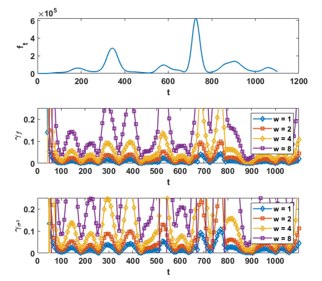
To demonstrate that and are indeed small, we calculate them for various window sizes over COVID-19 reported cases (Figure 2). Their values increase with larger (recall that the window size is ). For these calculations, we set . For small windows, the values are small, and so smoothing is advantageous. As expected, for large windows,the signal is oversmoothed resulting in higher values of and , consequently higher errors.
3 Results and Analysis
3.1 Synthetic Experiments
To evaluate our claims and analyze the effect of various variables, we ran an epidemic simulation in conjunction with the simulation of surveys over randomly generated networks111Our code is available at https://github.com/GCGImdea/coronasurveys/tree/master/papers/2024-AAAI-Nowcasting-Temporal-Trends-Using-Indirect-Surveys. .
Epidemic simulation
We use an extended SIR model to simulate an epidemic with varying infection parameters. The infection parameter starts at a value so that the reproduction number R0 (Dietz 1993) is above 2. At random times, we introduce “interventions” that reduce R0 smoothly to a value below 1. We run several such simulations and pick one that produces multiple peaks over 600 days, to emulate complex realistic epidemics like Influenza and COVID-19 that have multiple waves. We acknowledge that, in reality, not all infections will be detectable. However, assuming that each infection will be detected with a fixed probability only scales the time-series by a constant. Therefore, for the purpose of this study, we directly use to compute the hidden population over time.
Survey simulation
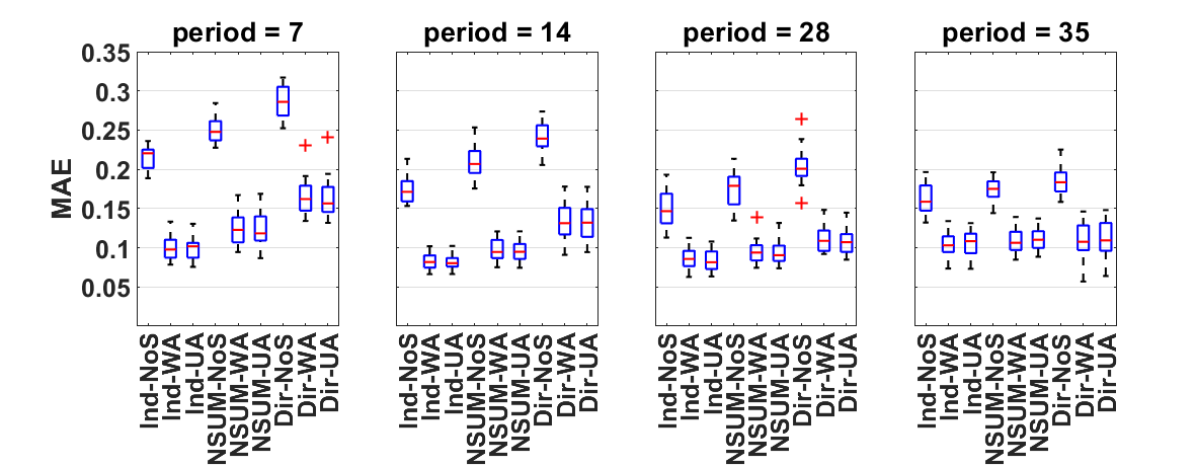
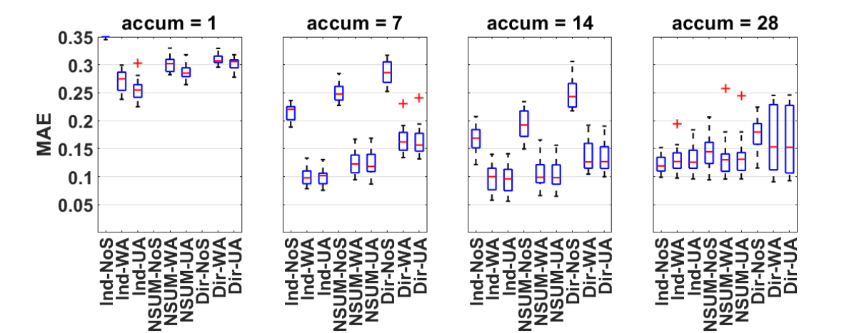
We simulate sampling nodes (respondents) from a graph with a power law distribution , with a bounded maximum degree, such that the mean degree is approximately a parameter . The choice of distribution was driven by the intention to introduce some skewness in the degree distribution to push the limits of our approach. The main conclusions do not change on Erdos-Renyi graphs. The simulation has the following parameters. (i) : approximate average degree in the latent graph; (ii) : upper limit on the number of individuals who respond on a given day. The actual number is uniformly selected from to ; (iii) : number of nodes that can potentially be covered by the respondents; (iv) accum: number of days over which the responses are accumulated ; (v) period: time window within which the respondents are to count the hidden population. E.g., if the question is “how many people do you know who have had COVID-like illnesses in the last 7 days,” then period . For each combination of the above parameters, we ran 16 simulations resulting in 82,000 combinations of parameters and simulations. For indirect surveys, we randomly infect each neighbor of the responders with the probability and obtain the indirect response from each responding node. We then accumulate the responses obtained over accum number of days. For comparison, we also introduced the traditional NSUM approach (Killworth et al. 1998a), where the response from each node is normalized by its degree. For direct surveys, we infect nodes among the responders and note the number of infections produced.
Results
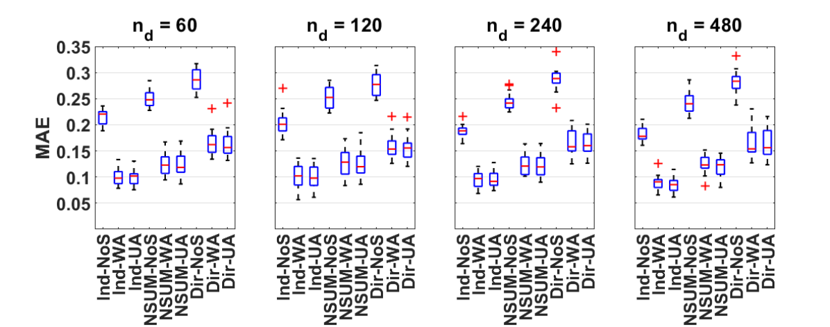
For each of indirect (Ind), NSUM, and direct (Dir) survey methods, we introduced the following post-processing methods: (1) NoS: Average response for each time unit (defined by accum) without any smoothing. (2) WA: Moving average of NoS weighted by the number of responses over a window . (3) UA: Unweighted moving average of NoS over a window . These methods were compared against the infections using MAE with time granularity redefined by the choice of accum. Before computing the error, we apply a range normalization, so that the maximum of each time-series is set to 1 and the minimum to 0. Note that here, is not the same as . To construct we would count the number of infections in the last period number of days. Secondly, note that setting the parameter accum is equivalent to performing a weighted average (scaled by a constant factor). Therefore, accum and will have a similar effect as using on accum .
Figure 3 shows the result of the survey simulation with parameters and . Time-series obtained from smoothed indirect survey is much more similar to the true infections compared to those obtained from direct surveys. The time-series of smoothed NSUM is also close to the true infections, but at times, worse than our indirect method.
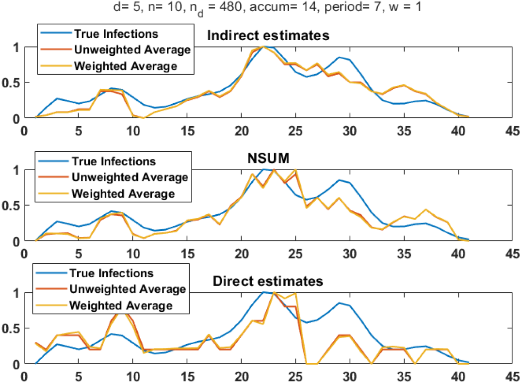
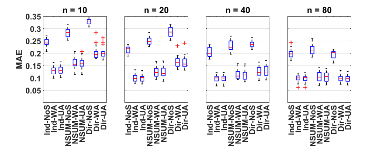
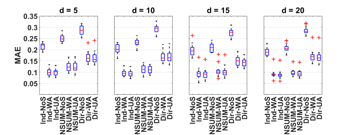
Figure 4 shows the distribution of errors obtained by different methods. In this figure, to focus on the impact of one parameter, we fix the others (, , , , , and ). In general, we note that the indirect methods (Ind-*) produce lower median errors than NSUM-* the direct methods (Dir-*). Also, there is no significant difference between weighted and unweighted smoothing strategies. In terms of parameters, the choice of and do not impact the relative patterns across the 9 methods (see Supplementary Material in full version (Srivastava et al. 2023)). As expected from our analysis (Theorems 3 and 4), increasing first decreases the errors, but a high value worsens the performance for the moving averages (*-UA, *-WA). A similar observation can be made for increasing – *-NoS which has produces a higher error than . All moving averages become similar as increases to .

3.2 Real Dataset
The objective of these experiments is to evaluate the performance of the proposed approach using datasets drawn from the US COVID-19 Trends and Impact Survey (CMU-CTIS) (Salomon et al. 2021). It has data on self-reported symptoms, symptoms in the respondent’s community, testing, isolation measures, vaccination acceptance, and mental health, among other factors, to assess the spread of COVID-19. Approximately 40,000 US respondents participated in this survey daily between April 6, 2020, and June 25, 2022. We chose the period of September 8, 2020, through March 1, 2022 because CMU-CTIS included in it a question regarding individual COVID-19 positive test results, which is used to estimate the direct survey results. A null value detection and removal, as well as an outlier filter are applied to the dataset for each state.
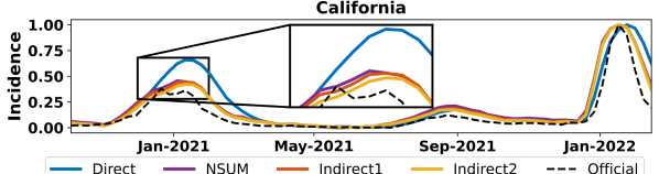
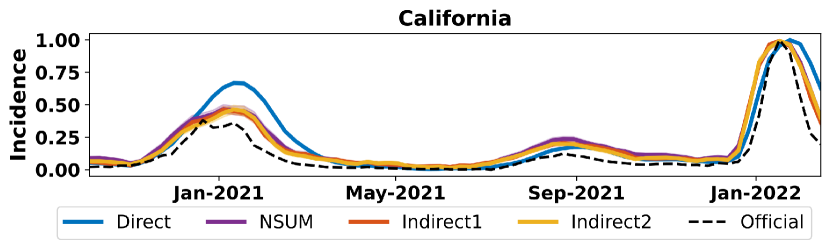
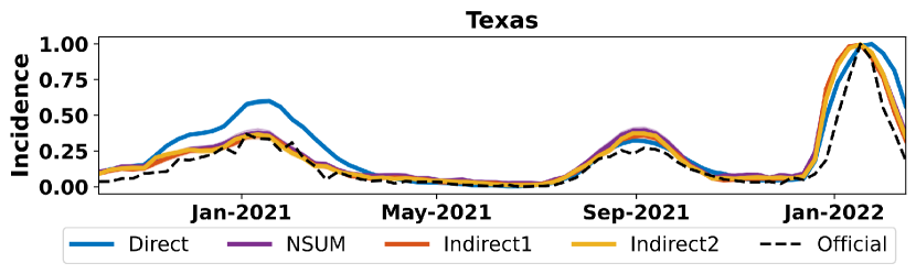
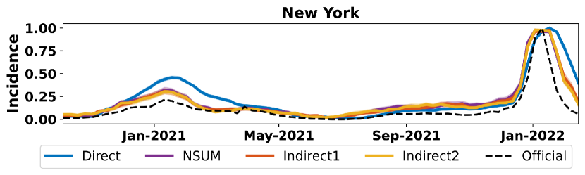
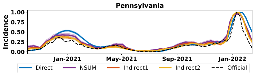
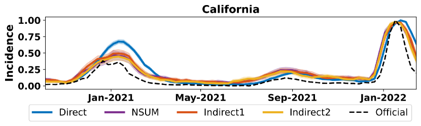
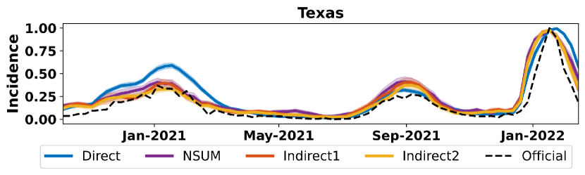
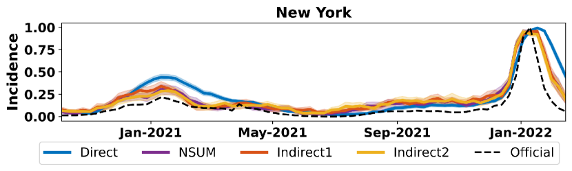
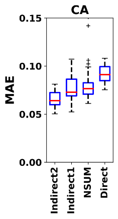
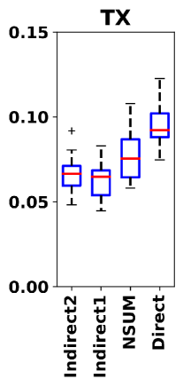
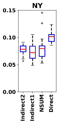
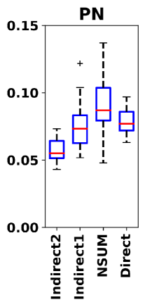
Figure 5 shows the normalized COVID-19 incidence curves from direct and indirect surveys for California from September 2020 to March 2022. For the curves derived from indirect surveys, we included both the CLI incidence reported in the household (Indirect1) and the CLI incidence reported within the local community (Indirect2). In addition, Figure 5 displays the curve obtained by the NSUM method (Killworth et al. 1998a) using household questions (CTIS has a question asking for the size of the household). For these curves, we set the parameters to and . For comparison purposes, we include the normalized incidence curves obtained from datasets provided by the Johns Hopkins Coronavirus Resource Center (Dong, Du, and Gardner 2020). We observe that the curves obtained from indirect surveys are much similar to the official ones. To quantitatively evaluate the proposed approach, Table 1 shows the MAE of the normalized incidence curves obtained from direct, NSUM and indirect surveys conducted in California, Texas, New York, and Pennsylvania for a variety of values of and . The reference curves are based on official data. For each (, ) pair, a bold font, and underlined values correspond to the best and the second-best values, respectively. As given in Table 1, the incidence curves obtained from indirect surveys exhibit lower MAE values than those obtained by both NSUM and direct approaches. Furthermore, the MAE values obtained from indirect surveys in the local community (Indirect2) are generally lower than those extracted from indirect surveys in the household (Indirect1).
| state | Direct | NSUM | Indirect1 | Indirect2 | ||
|---|---|---|---|---|---|---|
| 7 | 1 | CA | 0.0703 | 0.0443 | 0.0341 | 0.0292 |
| TX | 0.0661 | 0.0379 | 0.0289 | 0.0270 | ||
| NY | 0.0785 | 0.0315 | 0.0301 | 0.0299 | ||
| PN | 0.0572 | 0.0368 | 0.0300 | 0.0263 | ||
| 3 | CA | 0.1148 | 0.0988 | 0.0881 | 0.0811 | |
| TX | 0.1236 | 0.0890 | 0.0813 | 0.0782 | ||
| NY | 0.1210 | 0.0930 | 0.0910 | 0.0886 | ||
| PN | 0.0956 | 0.0907 | 0.0816 | 0.0691 | ||
| 14 | 1 | CA | 0.0836 | 0.0624 | 0.0524 | 0.0477 |
| TX | 0.0779 | 0.0385 | 0.0343 | 0.0336 | ||
| NY | 0.0929 | 0.0520 | 0.0504 | 0.0500 | ||
| PN | 0.0689 | 0.0389 | 0.0391 | 0.0429 | ||
| 3 | CA | 0.1441 | 0.1217 | 0.1116 | 0.1059 | |
| TX | 0.1349 | 0.1058 | 0.1042 | 0.1027 | ||
| NY | 0.1571 | 0.1165 | 0.1126 | 0.1090 | ||
| PN | 0.1349 | 0.1182 | 0.1110 | 0.1005 |
4 Discussion
Survey Design.
Our assumptions and results can be used to design better indirect surveys. As lower variance in the degree distribution is desirable due to Theorem 2, the question can be framed in a way to keep the variance low. For instance, instead of simply asking “how many people do you know who ”, we could restrict the set of people to be counted – “Among your and your two immediate neighboring households, how many do you know who .”
Targeted Surveys.
Our approach allows the responses to be from a restricted subset of the population. This is advantageous for targeted surveys. For instance, healthcare workers are more likely to know of Influenza hospitalizations than the general public. Therefore, we can restrict the survey to them to estimate the number of hospitalizations over time. Further, any direct survey on an online platform can only estimate the hidden subpopulation among those using the platform. Instead, an indirect survey will cover all the neighbors of the platform users in the latent graph.
Extension to Biased Reporting
In this paper we have assumed that the survey responses are honest and correct. However, in reality, the reporting could be biased to exaggerate counts or undercount, or the respondents may incorrectly recall. A detailed analysis of bias is beyond the scope of this paper. However, it can be shown that all our results apply if the respondents have different biases that underestimate or overestimate at the same rate over time – these biases scale the estimate by a constant factor. These results do not take into account respondents who are malicious, deliberately inaccurate (possibly due to the sensitivity of the questions), or exhibit other behaviors. In practice, additional steps can be taken to handle different biases (Scheers 1992; Kazemzadeh et al. 2016; Ezoe et al. 2012; Salganik et al. 2011).
5 Conclusions
We have proposed a latent graph formulation to estimate the temporal trends in the size of a hidden population from indirect surveys, leading to better estimates than those achievable with direct surveys having the same number of responses. We leveraged the temporal dynamics of the underlying process and identified the conditions under which a weighted moving average of responses leads to better estimates compared to raw responses. We performed extensive simulations of a temporal process over which a simulated survey is performed, to study the impact of various parameters on the estimation error. We demonstrated that our approach outperforms traditional Network Scale-Up Methods and the direct approach with and without performing a moving average. We also demonstrated that our approach is able to better estimate the trend of COVID-19 cases on real-world surveys over time.
Acknowledgements
This work was partially supported by grants TED2021-131264B-I00 (SocialProbing) and PID2019-104901RB-I00, funded by MCIN/AEI/10.13039/501100011033 and the European Union “NextGenerationEU”/PRTR. The authors would like to thank Mohamed Kacem for his contribution to pre-processing the data used in this work.
Ethical Declaration
The Ethics Board (IRB) of IMDEA Networks Institute approved this work on 2021/07/05. IMDEA Networks has signed Data Use Agreements with Facebook and Carnegie Mellon University (CMU) to access their data. Specifically, CMU project STUDY2020_00000162 entitled ILI Community-Surveillance Study. Informed consent has been obtained from all participants in this survey by this institution. All the methods in this study have been carried out in accordance with relevant ethics and privacy guidelines and regulations.
Availability of Data and Materials
The data presented in this paper (in aggregated form) and the codes used to process it will be made publicly available at https://github.com/GCGImdea/coronasurveys/tree/master/papers/2024-AAAI-Nowcasting-Temporal-Trends-Using-Indirect-Surveys. The microdata of the CTIS survey from which the aggregated data was obtained cannot be shared, as per the Data Use Agreements signed with Facebook and Carnegie Mellon University (CMU).
References
- Alix-Garcia, Sims, and Costica (2021) Alix-Garcia, J. M.; Sims, K. R.; and Costica, L. 2021. Better to be indirect? Testing the accuracy and cost-savings of indirect surveys. World Development, 142: 105419.
- Astley et al. (2021) Astley, C. M.; et al. 2021. Global monitoring of the impact of the COVID-19 pandemic through online surveys sampled from the Facebook user base. Proceedings of the National Academy of Sciences, 118(51).
- Bernard et al. (1989) Bernard, H. R.; Johnsen, E. C.; Killworth, P. D.; and Robinson, S. 1989. Estimating the Size of an Average Personal Network and of an Event Subpopulation. In The Small World, 159–175.
- Bhatia and Davis (2000) Bhatia, R.; and Davis, C. 2000. A better bound on the variance. The american mathematical monthly, 107(4): 353–357.
- Breza et al. (2020) Breza, E.; Chandrasekhar, A. G.; McCormick, T. H.; and Pan, M. 2020. Using aggregated relational data to feasibly identify network structure without network data. American Economic Review, 110(8): 2454–84.
- Dietz (1993) Dietz, K. 1993. The estimation of the basic reproduction number for infectious diseases. Statistical methods in medical research, 2(1): 23–41.
- Dong, Du, and Gardner (2020) Dong, E.; Du, H.; and Gardner, L. 2020. An interactive web-based dashboard to track COVID-19 in real time. The Lancet infectious diseases, 20(5): 533–534.
- Dunbar (2010) Dunbar, R. 2010. How many friends does one person need? Dunbar’s number and other evolutionary quirks. Harvard University Press.
- Ezoe et al. (2012) Ezoe, S.; Morooka, T.; Noda, T.; Sabin, M. L.; and Koike, S. 2012. Population size estimation of men who have sex with men through the network scale-up method in Japan. PloS one, 7(1): e31184.
- Feehan and Salganik (2016) Feehan, D. M.; and Salganik, M. J. 2016. Generalizing the network scale-up method: a new estimator for the size of hidden populations. Sociological methodology, 46(1): 153–186.
- Garcia-Agundez et al. (2021) Garcia-Agundez, A.; et al. 2021. Estimating the COVID-19 prevalence in Spain with indirect reporting via open surveys. Frontiers in Public Health, 9: 658544.
- Geldsetzer (2020) Geldsetzer, P. 2020. Knowledge and perceptions of COVID-19 among the general public in the United States and the United Kingdom: a cross-sectional online survey. Annals of internal medicine, 173(2): 157–160.
- Jing et al. (2018) Jing, L.; Lu, Q.; Cui, Y.; Yu, H.; and Wang, T. 2018. Combining the randomized response technique and the network scale-up method to estimate the female sex worker population size: an exploratory study. Public health, 160: 81–86.
- Kazemzadeh et al. (2016) Kazemzadeh, Y.; Shokoohi, M.; Baneshi, M. R.; and Haghdoost, A. A. 2016. The frequency of high-risk behaviors among Iranian college students using indirect methods: network scale-up and crosswise model. International journal of high risk behaviors & addiction, 5(3).
- Killworth et al. (1998a) Killworth, P. D.; Johnsen, E. C.; McCarty, C.; Shelley, G. A.; and Bernard, H. R. 1998a. A social network approach to estimating seroprevalence in the United States. Social networks, 20(1): 23–50.
- Killworth et al. (1998b) Killworth, P. D.; McCarty, C.; Bernard, H. R.; Shelley, G. A.; and Johnsen, E. C. 1998b. Estimation of seroprevalence, rape, and homelessness in the United States using a social network approach. Evaluation review, 22(2): 289–308.
- Laga, Bao, and Niu (2021) Laga, I.; Bao, L.; and Niu, X. 2021. Thirty years of the network scale-up method. Journal of the American Statistical Association, 116(535): 1548–1559.
- Oliver et al. (2020) Oliver, N.; et al. 2020. Assessing the impact of the COVID-19 pandemic in Spain: large-scale, online, self-reported population survey. Journal of medical Internet research, 22(9): e21319.
- Rossier (2010) Rossier, C. 2010. The anonymous third party reporting method. Methodologies for estimating abortion incidence and abortion-related morbidity: a review, 99–106.
- Salganik et al. (2010) Salganik, M.; et al. 2010. Estimating the number of heavy drug users in Curitiba, Brazil using multiple methods. Technical report, Technical report. UNAIDS.
- Salganik et al. (2011) Salganik, M. J.; et al. 2011. The game of contacts: estimating the social visibility of groups. Social networks, 33(1): 70–78.
- Salomon et al. (2021) Salomon, J. A.; et al. 2021. The US COVID-19 Trends and Impact Survey: Continuous real-time measurement of COVID-19 symptoms, risks, protective behaviors, testing, and vaccination. Proceedings of the National Academy of Sciences, 118(51): e2111454118.
- Scheers (1992) Scheers, N. 1992. A review of randomized response techniques. Measurement and Evaluation in Counseling and Development.
- Srivastava et al. (2023) Srivastava, A.; Ramirez, J. M.; Diaz, S.; Aguilar, J.; Ortega, A.; Fernandez-Anta, A.; and Lillo-Rodriguez, R. 2023. Estimating Temporal Trends using Indirect Surveys. arXiv preprint arXiv:2307.06643.
- Teo et al. (2019) Teo, A. K. J.; et al. 2019. Estimating the size of key populations for HIV in Singapore using the network scale-up method. Sexually transmitted infections, 95(8): 602–607.
Supplementary Material
Appendix A Proofs
Here we provide detailed proofs of all the Theorems and Lemmas used in the paper.
Proof of Theorem 1.
Let be the fraction of nodes with in-degree in . Consider a node partitioning graph into sets , where represents the set of all nodes of in-degree . By Assumption 1, for any belonging to the neighborhood of some , the indicator random variable of the event is independent of , i.e., . Now, if we pick a random node from for the indirect survey, due to linearity of expectation,
| (4) | ||||
| (5) |
When we randomly select a node in , . By the law of total expectation,
| (6) | ||||
| (7) |
∎
Proof of Lemma 1.
We wish to compute the variance using . We already have . By the law of total expectation, .
| (8) | ||||
| (9) | ||||
| (10) |
Since, and are non-negative, and ,
| (11) |
Proof of Theorem 2.
By Lemma 2,
| (13) |
where is the error function, and the equation follows from the fact that follows standard normal distribution. Similarly,
| (14) |
Suppose, the probability of deviation is higher from the indirect estimate. Then, from Equations 13 and 14,
Since, is an increasing function,
| (15) |
Putting the value of from Lemma 1, combining with Equation 15, after some algebraic manipulations gives
| (16) |
Hence, if , then . ∎
Proof of Lemma 3.
Proof of Lemma 4.
Let . Since, , we have
And,
More generally,
Telescoping the above to , we get
Since, , we get
Where . Telescoping again down to , we get
| (20) |
for , and
We can prove that
| (21) |
We omit the details for brevity. The idea is to use induction with base case for which . Therefore,
Repeating the above analysis replacing with and reversing all inequalities,
which completes the proof. ∎
Proof of Lemma 5.
By using triangle inequality, followed by the bound on , we have
Using this inequality, we get
| (22) | |||
| (23) |
Equation 22 follows from the fact that , being a linear combination of normally distributed variables, also follows a normal distribution. ∎
Proof of Theorem 3.
Now,
| (26) | ||||
| (27) | ||||
| (28) |
∎
Proof of Lemma 6.
| [By Lemma 4] | |||
| [Since ] | |||
| [By Cauchy-Schwarz Inequality] | |||
| (29) | |||
| (30) |
Setting ,
| (31) |
Similarly, we can show
| (32) |
∎
Proof of Theorem 4.
A.1 Extension to Biased Reporting
In this paper, we have assumed that the response is honest and correct. However, in reality, the reporting could be biased to exaggerate counts or undercount, or the respondents may incorrectly recall. Suppose, the bias follows the following pattern.
Assumption 4.
The respondents can be grouped, where an individual belongs to the group with probability (independently of its in-degree) and overestimates the hidden population by a factor of (underestimates if ¡ 1). Also, and are constants over time.
Suppose is a randomly selected response with possible bias following Assumption 4 and is the sample mean. Then
Theorem 5.
, , and for any
| (34) |
where .
Proof.
The expectation of response from a randomly selected person is given by
| (35) |
where . This suggests that consistent biases among the groups scales the time-series of expected responses by a constant Similarly, we can show that . Considering the probability of a certain deviation obtained by scaling of the sample mean :
| (36) | |||||
which is identical to the expression in Equation 14 where bias is absent. ∎
Therefore, all of our results still apply after normalizing the time-series of and even if there are biases in the responses under Assumption 4.
The above analysis does not take into account respondents who are malicious, deliberately inaccurate (possibly due to the sensitivity of the questions), or exhibit other behaviors that deviate from Assumption 4. In practice, additional steps can be taken to handle these different biases (Scheers 1992; Kazemzadeh et al. 2016; Ezoe et al. 2012; Salganik et al. 2011).
Appendix B Additional Results
Testing Observation 1
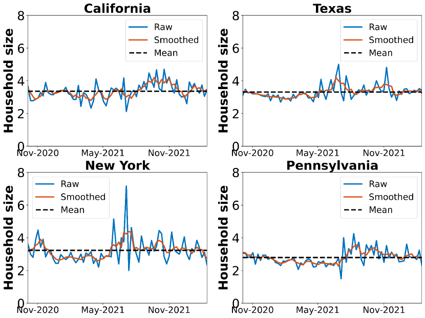
In our analysis, we indicated that the average degree of the latent graph remains roughly constant. The CMU-CTIS recorded indirect survey information on COVID-like illness (CLI) incidence both in the household and in the local community. Figure 6 shows the average household size obtained across time from four states (California, Texas, New York, and Pennsylvania). The average remains roughly constant, supporting Observation 1.
Undersampling Real Data
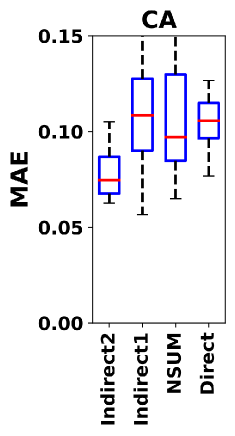
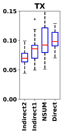
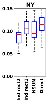
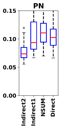
To demonstrate that our approach works with a small number of responses as well, we performed experiments where we undersampled the US CMU-CTIS data. Figure 7 displays the averaged COVID-19 incidence curves and the corresponding 95% confidence interval from direct and indirect surveys using 10% of the daily samples for the four states and for and . Specifically, the curves are the ensemble average of 25 realizations of the experiment, where a random subset of 10% of the daily samples was selected at each realization. As can be seen in this figure, the curves from direct and indirect surveys closely follow the trend of the curve obtained from official data. Fig. 9 illustrates the boxplots of errors obtained by the various methods using 10% of the daily samples for the four states and for and . As can be seen in these boxplots, the indirect methods yield the lower median errors compared to those obtained by NSUM and direct techniques. Figures 8 and 13 show, respectively the normalized incidence curves and the distributions errors using 3% of the daily samples for the four states and for and .
|
|
|
|
|
|
|

|
|
More Simulation Results
Here we present the boxplots omitted from the main paper showing the impact of and . These parameters had negligible impact.
B.1 Results on UMD surveys
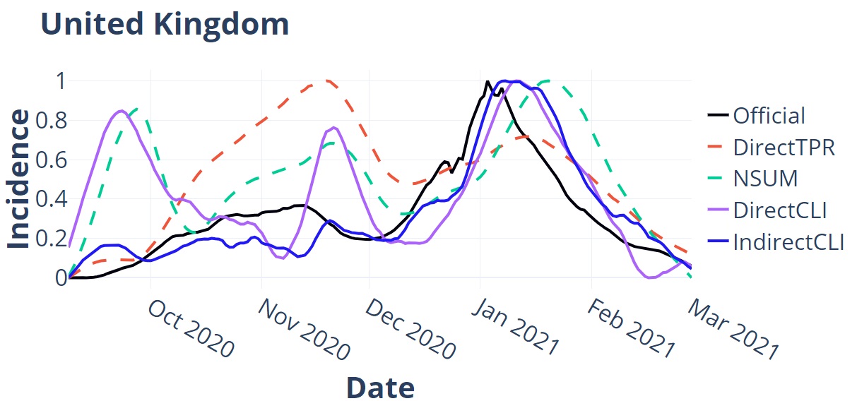
We also conducted experiments on UMD surveys 222https://covidmap.umd.edu/ that collected survey data at the country level for various countries. In this dataset, there are responses regarding if one has tested positive recently (DirectTPR), if they have COVID-like symptoms (DirectCLI), and the “indirect” question – how many they know who have COVID-like symptoms. The last question allows us to perform estimation using our approach (Indirect). We used , i.e., a window of to aggregate the responses. There is no information on the personal network size which is needed for NSUM. Therefore, we used an existing technique333https://arxiv.org/abs/2108.03284 that estimates the personal network size for comparison. The ground truth was obtained from the reported case count available from Our World in Data444https://ourworldindata.org/covid-cases. The results are presented in Table 2. We note that Indirect outperforms DirectCLI and NSUM on all countries with a significant margin in most. In fact, Indirect (regarding CLI) provides a better estimate than directly asking about positive tests in most countries. Figure 12 shows the comparison of estimated incidences for the United Kingdom. Our approach (IndirectCLI) most closely resembles the ground truth. Our estimates are not only better than DirectCLI but also better than asking directly about positive tests (as opposed to indirect on CLI).
| Country | DirectTPR | NSUM | DirectCLI | Indirect |
|---|---|---|---|---|
| Brazil | 0.14 | 0.17 | 0.15 | 0.15 |
| Canada | 0.14 | 0.19 | 0.4 | 0.12 |
| France | 0.17 | 0.24 | 0.22 | 0.13 |
| Germany | 0.1 | 0.19 | 0.29 | 0.12 |
| Israel | 0.32 | 0.19 | 0.17 | 0.12 |
| Italy | 0.17 | 0.13 | 0.05 | 0.1 |
| Japan | 0.15 | 0.23 | 0.25 | 0.08 |
| Spain | 0.31 | 0.2 | 0.16 | 0.1 |
| Turkey | 0.24 | 0.29 | 0.16 | 0.12 |
| UK | 0.24 | 0.26 | 0.23 | 0.11 |
Appendix C Additional Methodology Details
C.1 Code
All our code and aggregate datasets are publicly available555Our code is available at https://github.com/GCGImdea/coronasurveys/tree/master/papers/2024-AAAI-Nowcasting-Temporal-Trends-Using-Indirect-Surveys.. The synthetic experiments were run on a machine with Intel(R) Core(TM) i8 CPU, 3GHz, 6 cores, and 16GB RAM. The code was written in MATLAB 2021b. The experiments on real-world data were conducted on a machine with Intel(R) Xeon(R) CPU, 2.60GHz, 16 cores, and 32GB RAM. The pre-processing code to generate aggregate data from CTIS survey was written in R. The results demonstarted in the paper were generated using Python.
C.2 Outlier Filtering
In order to remove inconsistent and potentially malicious responses to the CTIS survey we apply a simple outlier filter based on the following rules:
-
•
We remove responses that report negative values in numeric questions that can only have non-negative responses.
-
•
We remove responses that report more than 100 in the number of people in household with COVID-like illness (CLI), in the number of people in the household in any age range (, 18-64, and ), or in the number of days with symptoms.
-
•
We remove inconsistent responses that report people in household with CLI but no symptoms, or report more people with CLI than the household size.
|
C.3 Synthetic Experiments
Here we present more details on the simulations.
Epidemic simulation
We use a simple SIR model to simulate an epidemic with varying infection parameters whose reproduction number R0 (Dietz 1993) is above 2. At random points in time, we introduce “interventions” that reduce R0 smoothly to a value below 1. We run several such simulations and pick one that produces multiple peaks over 600 days, to emulate realistic epidemics like Influenza and COVID-19 that have multiple waves. We acknowledge that, in reality, not all infections will be detectable. However, assuming that each infection will be detected with a fixed probability only scales the time-series (the number of infectious individuals by the SIR process) by a constant. Therefore, for the purpose of this study, we directly use to compute the hidden population over time.
Survey simulation.
We simulate, at each time , random sets and of sizes and , and a bipartite digraph between them with terminal set , which represents the surveyed individuals. To construct the digraph, we pick the degree of vertex , from a power law distribution , such that mean degree is approximately . The choice of the probability distribution was driven by the intention to introduce some skewness in the degree distribution. Then, we add an edge between and with a probability .
For the indirect surveys simulation, we randomly infect each node in with the probability , where period is the time window within which the respondents are to count the hidden population. For comparison, we also introduced the traditional NSUM approach (Killworth et al. 1998a), where the response from each node is normalized by its degree. For direct surveys, we infect nodes in itself and note the number of infections produced in .
Appendix D Algorithm in Practice
Suppose we have some bounds on and . This could be obtained from prior experience. For example, if we are estimating the number of people who test positive for COVID-19, we can use prior trend of COVID-19 when the reporting quality was better (before home tests). We can use these along with Theorems 3 and 4 to identify a window that is likely to improve our estimation as given in Algorithm 1. Suppose we are given a threshold acceptable fractional deviation, e.g., . Then we can search for a that either satisfies Inequality 2 or Inequality 3. If Inequality 2 is satisfied, then by Theorem 3, aggregating with window must be better than no smoothing. If Inequality 3, then the same applies due to Theorem 4. We can apply this aggregation over discrete bins (daily, weekly, monthly) or in a rolling fashion (smoothing), or some combination of the two.