Acoustic dipole surfing on its own acoustic field: toward acoustic quantum analogues.

Abstract

In a recent paper [J. Fluid Mech., 952: A22 (2022)], Roux et al. demonstrated that a translating monopolar acoustic source is subjected to a self-induced radiation force opposite to its motion. This force results from a symmetry breaking of the emitted wave induced by Doppler effect. In the present work, we show that for a dipolar source, the self-induced radiation force can be aligned with the velocity perturbation, hence amplifying it. This work suggests the possibility of a dipolar acoustic source surfing on its own acoustic wave, hence paving the way towards acoustic quantum analogues.

Keywords : acoustic radiation force - dipole - quantum analogues

1 Introduction

In their seminal experiments, [Couder et al.(2005)] unveiled a classical hydrodynamic system exhibiting a wave-particle duality. This system is made of a self-propelling drop driven by a resonant interaction with its own wavefield. This wavefield is created by a drop bouncing (without merging) at the surface of a bath excited just below the Faraday threshold ([Faraday(2022), Kumar & Tuckerman(1994)]) and giving birth to a localized wave intrinsically linked to its dual particle. With this system, researchers were able to reproduce a wealth of behaviors classically associated with the quantum realm such as: tunneling ([Eddi et al.(2009), Hubert et al.(2017), Nachbin et al.(2017)],[Tadrist et al.(2020)]), Landau levels ([Fort et al.(2010), Harris & Bush(2014), Oza et al.(2014)]), quantum coral ([Harris et al.(2013), Gilet(2014), Gilet(2016), Sáenz et al.(2018), Cristea-Platon et al.(2018)]) or Friedel oscillation ([Sáenz et al.(2020)]). An exhaustive list of the quantum analogies explored with these self-propelling drops can be found in the recent review by [Bush & Oza(2020)].

While this system has considerably contributed to the development of the field of classical quantum analogues, it also has some inherent limitations. For example, the possibilities and limits of these hydrodynamic quantum analogues to reproduce the iconic double-slits experiment have been thoroughly explored by [Andersen et al.(2015), Dubertrand et al.(2016), Faria(2017), Pucci et al.(2018), Rode et al.(2019), Ellegaard & Levinsen(2020)] after the initial experimentation by [Couder & Fort(2006)]. More generally, (i) hydrodynamic quantum analogues are only 2D by nature, while quantum mechanics is inherently 3D. (ii) The influence of the hydrodynamic pilot wave through memory effects is limited by viscous damping. Third, only monopolar bath vibrations can be created by the droplet bouncing, excluding the exploration of other modes. Finally, the system requires a periodic disconnection between the particle and its wave in an additional spatial dimension, that cannot exist in a 3D system.

Acoustic quantum analogues could provide an elegant solution to some of these limitations. Indeed, it is known since the early work by [Rayleigh(1905)], [Brillouin(1925)] and Langevin (work reported later on by [Biquard(1932a), Biquard(1932b)]), that an acoustic scatterer excited by an acoustic field is subjected to a nonlinear force called the acoustic radiation force. This force results from intrinsic nonlinearities of Navier-Stokes equations and another nonlinearity resulting from the integration of the stress exerted by the acoustic wave on a vibrating surface ([Brillouin(1925)]). The acoustic radiation force can be used to remotely trap and manipulate objects (see e.g. the review by [Baudoin & Thomas(2020)]). This has led to the development of standing-wave based and vortex based selective acoustical tweezers ([Marzo et al.(2015), Baresch et al.(2016), Riaud et al.(2017), Baudoin et al.(2019), Baudoin et al.(2020)]), with a renewed interest in the last century to manipulate millimeter down to micrometer scale objects both in vitro and in vivo ([Rufo et al.(2022)]). This interest in acoustic manipulation has also led to some recent theoretical developments to compute the radiation force ([Silva(2011), Baresch et al.(2013), Sapozhnikov & Bailey(2013), Gong & Baudoin(2021)]) and torque ([Silva et al.(2012), Gong & Baudoin(2020)]) exerted by an arbitrary acoustic field on a spherical particle.

Yet, the emergence of an acoustic wave-particle duality requires that the acoustic source is moved by its own acoustic field, not by an incident field. Also ideally, the direction of motion of the source should not be set a priori by an anisotropy of the radiated field. For symmetry reasons one can nevertheless easily figure out that an isotropic acoustic field cannot give birth to a directional self-induced radiation force. Recently, [Roux et al.(2022)] demonstrated theoretically that adding a slight translation perturbation to a monopolar source induces a symmetry breaking due to Doppler effect and hence a directional acoustic radiation force. But in this case, the force was opposite to the velocity perturbation, hence leading to a stable configuration. Here we compute the self-induced radiation force exerted on a dipolar source. We show that depending on the orientation of the dipole compared to the velocity perturbation, the radiation force can be oriented in the same direction as the velocity perturbation, hence amplifying it. This unstable situation paves the way towards acoustic sources driven by their own acoustic field, a situation analogous to the one at the origin of hydrodynamic quantum analogues. Note that this situation is reminiscent of some recent discoveries of hydrodynamic surfers driven by they own capillary and gravity waves ([Ho et al.(2021), Benham et al.(2022)]), though in these cases, the direction of motion is set a priori by the orientation of the source.

2 Dipolar source

The calculation of the acoustic radiation force for a dipolar source follows the same essential steps as the ones used previously to compute it for a monopolar source ([Roux et al.(2022)]), but with an additional degree of complexity induced by the vectorial nature of the source and the orientation between the source and the translation direction.

The first step is to model the dipolar source. In acoustics, a fixed punctual dipolar source can be seen as a punctual volumetric source of force:

$$\mathbf{f_{v}}(\mathbf{r},t)=\mathbf{f}(t)\cdot\delta(x)\cdot\delta(y)\cdot\delta(z),$$

with $t$ and $(x,y,z)$ the time and Cartesian coordinates associated with a Galilean reference frame $\mathcal{R}=(O,(x,y,z),t)$, $\delta$ the Dirac delta function, $\mathbf{r}=(x,y,z)$ the position vector and $\mathbf{f}$ the vector function specifying the time dependence of the the volumetric force. If we consider a small translation perturbation of this source under the form of a constant speed $\mathbf{U}=Mc\;\mathbf{x}$ along the axis $Ox$ (Fig.1), with $M\ll 1$ the Mach number and $c$ the sound speed, the translating source can be modeled by the source term:

$$\mathbf{f_{v}}(\mathbf{r},t)=\mathbf{f}(t)\cdot\delta(x-Mct)\cdot\delta(y)\cdot\delta(z).$$ (1)

For the sake of generality, the direction of the dipolar source is supposed to be arbitrary, leading to the general expression:

$$\mathbf{f}(t)=F\sin(\omega t)\begin{pmatrix}c_{x}\\ c_{y}\\ c_{z}\\ \end{pmatrix}$$ (2)

with $\mathbf{c}=\begin{pmatrix}c_{x}\\ c_{y}\\ c_{z}\end{pmatrix}$ a unit vector $(\|\mathbf{c}\|=1)$, $F$ the force amplitude, $\omega$ the angular frequency and $\|\mathbf{.}\|$ the Euclidean norm operator.

3 Wavefield radiated by a translating dipolar source

3.1 Wave equation

The wavefield radiated by a translating dipolar source can be computed by solving the linearized Euler equations (mass and momentum balances):

$$\frac{\partial\rho_{1}}{\partial t}+\rho_{0}\cdot\mathrm{\nabla\cdot}(\mathbf{v_{1}})=0,$$ (3a)

$$\rho_{0}\frac{\partial\mathbf{v_{1}}}{\partial t}+\nabla p_{1}-=\mathbf{f}(t)\cdot\delta(x-Mct)\cdot\delta(y)\cdot\delta(z),$$ (3b)

with $\rho_{1}$, $p_{1}$ and $\mathbf{v_{1}}$ the first order perturbations in density, pressure and velocity respectively, and $\rho_{0}$ the density at rest. In addition, the linearized equation of state for an inviscid fluid reads: $p_{1}/\rho_{1}=c^{2}$ with $c$ the sound speed.

(i) Subtracting $c$ times the gradient of eq. (3a) to the time derivative of eq. (3b), (ii) taking into account the equation of state $p_{1}/\rho_{1}=c^{2}$ and the irrotational nature of the acoustic wavefield leading to $\nabla(\mathrm{\nabla\cdot}\mathbf{v_{1}})=\Delta\mathbf{v_{1}}$, (iii) introducing the acoustic displacement $\mathbf{u_{1}}$ such that $\mathbf{v_{1}}=\frac{\partial\mathbf{u_{1}}}{\partial t}$ and (iv) integrating the resulting equation over time leads to the classic wave equation for the displacement with the dipolar source on the rhs:

$$\frac{\partial^{2}\mathbf{u_{1}}}{\partial t^{2}}-c^{2}\Delta\mathbf{u_{1}}=\frac{1}{\rho_{0}}\mathbf{f}(t)\cdot\delta(x-Mct)\cdot\delta(y)\cdot\delta(z)\;.$$ (4)

3.2 Lorentz transformation

Using the Lorentz invariance of the wave equation, this equation can be rewritten in a reference frame wherein the source is fixed with the following change of variables:

$$x^{\prime}=\gamma(x-Mct)$$ (5a)

$$y^{\prime}=y$$ (5b)

$$z^{\prime}=z$$ (5c)

$$ct^{\prime}=\gamma(ct-Mx)$$ (5d)

where $\gamma=\frac{1}{\sqrt{1-M^{2}}}$. This Lorentz transform allows to rewrite equation (4) into:

$$\frac{\partial^{2}\mathbf{u_{1}}}{\partial t^{\prime 2}}-c^{2}\Delta^{\prime}\mathbf{u_{1}}=\frac{1}{\rho_{0}}\mathbf{f}\left(\frac{\gamma}{c}\left(ct^{\prime}+Mx^{\prime}\right)\right)\delta\left(\frac{x^{\prime}}{\gamma}\right)\delta(y^{\prime})\delta(z^{\prime}).$$ (6)

We can see that for any $x^{\prime}\neq 0$, the rhs term is null, which means that we can consider it only when $x^{\prime}=0$. If we combine this with the fact that $\delta\left(\frac{x^{\prime}}{\gamma}\right)=\gamma\delta(x^{\prime})$, we can write:

$$\frac{\partial^{2}\mathbf{u_{1}}}{\partial t^{\prime 2}}-c^{2}\Delta^{\prime}\mathbf{u_{1}}=\frac{\gamma}{\rho_{0}}\mathbf{f}(\gamma t^{\prime})\delta(x^{\prime})\delta(y^{\prime})\delta(z^{\prime}).$$ (7)

This equation can be further simplified using the second transform:

$$x^{\prime\prime}=\gamma x^{\prime}$$ (8a)

$$y^{\prime\prime}=\gamma y^{\prime}$$ (8b)

$$z^{\prime\prime}=\gamma z^{\prime}$$ (8c)

$$ct^{\prime\prime}=\gamma ct^{\prime}$$ (8d)

leading to the final equation:

$$\Delta^{\prime\prime}\mathbf{u_{1}}-\frac{1}{c^{2}}\frac{\partial^{2}\mathbf{u_{1}}}{\partial t^{\prime\prime 2}}=-\frac{\gamma^{2}}{c^{2}\rho_{0}}\mathbf{f}(t^{\prime\prime})\delta(x^{\prime\prime})\delta(y^{\prime\prime})\delta(z^{\prime\prime}).$$ (9)

3.3 Solutions of the equation

The solution of the wave equation for a fixed punctual source is well known (see e.g. [Morse & Ingard(1968)]):

$$\mathbf{u_{1}}=\displaystyle\frac{\gamma^{2}}{c^{2}\rho_{0}}\frac{\mathbf{f}\left(t^{\prime\prime}\pm\frac{r^{\prime\prime}}{c}\right)}{4\pi r^{\prime\prime}},$$ (10)

which becomes with the initial variables (see the details in [Roux et al.(2022)]):

$$\boxed{\mathbf{u_{1}}=\frac{\mathbf{f}\left(t-\frac{R}{c}\right)}{4\pi c^{2}\rho_{0}R_{1}},}$$ (11)

with $R=\frac{M(x-Mct)+R_{1}}{1-M^{2}}$ the distance between the emission and observation points and:

$$R_{1}=\sqrt{(x-Mct)^{2}+(y^{2}+z^{2})(1-M^{2})}.$$ (12)

4 Expression of the radiation force in the far field

Figure 1: Sketch of the problem. $\mathcal{R}=(O,(x,y,z),t)$ is a Galilean reference frame. $\mathbf{U}$ corresponds to the velocity translation of the dipolar source and $\mathcal{R}^{*}=(O,(x,^{*}y^{*},z^{*}),t)$ to a reference frame linked to the source. The surface $\mathcal{S_{\infty}}$ is a spherical surface centered on the dipole, moving with it at the velocity $\mathbf{U}$ in $\mathcal{R}$ and with a radius $r_{\infty}$ much larger than all other characteristic length of the problem.

Now that we have determined the field radiated by the translating dipolar source, the next step is to compute the self radiation force acting on it. The radiation force exerted on an object is by definition the time average of the stress integrated over the surface $S(t)$ of this object:

$$\left<\mathbf{F_{rad}}\right>=\left<\iint_{\mathcal{S}(t)}\overline{\overline{\sigma}}\;\mathbf{n}\;\mathrm{d}S\right>,$$ (13)

with $\overline{\overline{\sigma}}$ the stress tensor, $\mathbf{n}$ a unit vector normal to the integration surface, $\mathrm{d}S$ an infinitesimal surface and $\left<f\right>$ the time average of a time-dependant periodic function $f$ over its period. Such integration is difficult to perform directly since generally the surface $\mathcal{S}(t)$ of the object is moving. In addition, this expression is not tractable in the punctual source approximation. Hence, this integral is classically turned into an integral over a steady spherical surface in the far field $\mathcal{S_{\infty}}$ (i.e. with a radius $r_{\infty}$ much larger than all other characteristic length of the problem) encompassing the source by using the divergence and Reynold transport theorems (see e.g. the review by [Baudoin & Thomas(2020)]). Compared to the classical calculation, an additional difficulty is induced here by the translation of source. This problem was solved by [Roux et al.(2022)] by considering a spherical surface $\mathcal{S_{\infty}}$ centered on the source, and hence translating at the same velocity $\mathbf{U}$ as the source in $\mathcal{R}$, and adapting the classical calculation to this translating surface. This leads to the following integral expression of the radiation force expressed as a function of the first order acoustic field:

$$\boxed{\left<\mathbf{F}_{\text{rad}}\right>=\left<\iint_{\mathcal{S_{\infty}}}{\left[\left(\rho_{0}\frac{v_{1}^{2}}{2}-\frac{1}{\rho_{0}c^{2}}\frac{p_{1}^{2}}{2}\right)\bar{\bar{I}}-\rho_{0}\mathbf{v_{1}}\otimes\mathbf{v_{1}}\right]}\mathbf{n}dS\right>+\left<\iint_{\mathcal{S_{\infty}}}(\mathbf{U}\cdot\mathbf{n_{\infty}})\rho_{1}\mathbf{v_{1}}dS\right>.}$$ (14)

The first term corresponds to the classical integral expression of the radiation force on a steady surface at infinity, while the second term appears due to the translation of the surface $\mathcal{S_{\infty}}$.

5 Expression of the velocity, pressure and density fields in the far field.

The next step is to compute the velocity, pressure and density fields at first order in the far field to compute this integral.

5.1 Expression of the velocity, pressure and density fields

The expression of the velocity field can be simply obtained from the definition of the acoustic displacement:

$$\mathbf{v_{1}}=\frac{\partial\mathbf{u_{1}}}{\partial t}.$$ (15)

Then, the introduction of the acoustic displacement in the continuity equation (3a) leads to:

$$\frac{\partial\rho_{1}}{\partial t}+\frac{\partial}{\partial t}\Big{(}\rho_{0}\nabla\cdot\mathbf{u_{1}}\Big{)}=0,$$

which gives:

$$\rho_{1}=\frac{p_{1}}{c^{2}}=-\rho_{0}\nabla\cdot\mathbf{u_{1}}.$$ (16)

5.2 Far field approximation

To simplify the calculation of these expressions and of integral (14), we introduce the following change of variables:

$$\begin{cases}x^{*}&=x-Mct,\\ y^{*}&=y,\\ z^{*}&=z,\\ t^{*}&=t,\\ \end{cases}\qquad\text{and the associated spherical coordinates:}\qquad\begin{cases}x^{*}&=r^{*}\cos\theta^{*},\\ y^{*}&=r^{*}\sin\theta^{*}\cos\phi^{*},\\ z^{*}&=r^{*}\sin\theta^{*}\sin\phi^{*},\\ \end{cases}$$

corresponding to the Galilean transformation from $\mathcal{R}$ to $\mathcal{R}^{*}=(O^{*},(x^{*},y^{*},z^{*}),t^{*})$ where $\mathcal{R}^{*}$ is the reference frame associated with the moving source.

Figure 2: Sketch illustrating the spherical coordinates $(r^{*},\theta^{*},\varphi^{*})$ of a point $P$ in $\mathcal{R}^{*}$.

Assuming that the dipole velocity is small compared to the speed of sound ($M\ll 1$) leads to the following expressions at first oder in $M$ ([Roux et al.(2022)]):

$$R_{1}=r^{*} +\mathscr{O}(M^{2})$$ (17a)

$$R=r^{*}(1+M\cos\theta^{*}) +\mathscr{O}(M^{2})$$ (17b)

We can also compute the derivatives of these terms, which will be used later on :

$$\frac{\partial R}{\partial t} \simeq-Mc(\cos\theta^{*}+M), \frac{\partial R_{1}}{\partial t} \simeq-Mc\cos\theta^{*},$$

$$\frac{\partial R}{\partial x^{*}} \simeq\cos\theta^{*}+M, \frac{\partial R_{1}}{\partial x^{*}} \simeq\cos\theta^{*},$$

$$\frac{\partial R}{\partial y^{*}} \simeq\sin\theta^{*}\cos\phi^{*}, \frac{\partial R_{1}}{\partial y^{*}} \simeq\sin\theta^{*}\cos\phi^{*},$$

$$\frac{\partial R}{\partial z^{*}} \simeq\sin\theta^{*}\sin\phi^{*}, \frac{\partial R_{1}}{\partial z^{*}} \simeq\sin\theta^{*}\sin\phi^{*}.$$

5.2.1 Velocity field

Developping equation (15) within the small Mach number approximation leads to:

$$\mathbf{v_{1}} = \frac{1}{4\pi c^{2}\rho_{0}}\left[\frac{1}{R_{1}}\frac{\partial\mathbf{f}\left(t-\frac{R}{c}\right)}{\partial t}-\frac{1}{R_{1}^{2}}\frac{\partial R_{1}}{\partial t}\mathbf{f}\left(t-\frac{R}{c}\right)\right]$$

$$\simeq \frac{1}{4\pi c^{2}\rho_{0}r^{*}}\left[\left(1-\frac{1}{c}\frac{\partial R}{\partial t}\right)\mathbf{f^{\prime}}\left(t-\frac{R}{c}\right)-\frac{1}{r^{*}}\frac{\partial R_{1}}{\partial t}\mathbf{f}\left(t-\frac{R}{c}\right)\right]$$

$$\simeq \frac{1}{4\pi c^{2}\rho_{0}r^{*}}\left[(1+M\cos\theta^{*})\mathbf{f^{\prime}}\left(t-\frac{R}{c}\right)+\frac{Mc\cos\theta^{*}}{r^{*}}\mathbf{f}\left(t-\frac{R}{c}\right)\right],$$

which can be simplified in the far field approximation into:

$$\boxed{\mathbf{v_{1}}\simeq\frac{1+M\cos\theta^{*}}{4\pi c^{2}\rho_{0}r^{*}}\mathbf{f^{\prime}}\left(t-\frac{R}{c}\right).}$$ (18)

5.2.2 Pressure field

Doing similar developments for the pressure field starting from Eq. (16) leads to:

$$p_{1} = -\frac{1}{4\pi}\nabla\cdot\frac{\mathbf{f}\left(t-\frac{R}{c}\right)}{R_{1}}$$

$$\simeq -\frac{1}{4\pi R_{1}^{2}}\left[R_{1}\nabla\cdot\mathbf{f}\left(t-\frac{R}{c}\right)-\mathbf{f}\left(t-\frac{R}{c}\right)\cdot\nabla R_{1}\right]$$

$$\simeq -\frac{1}{4\pi}\left[\frac{1}{r^{*}}\left(-\frac{1}{c}\right)\nabla R\cdot\mathbf{f^{\prime}}\left(t-\frac{R}{c}\right)-\frac{1}{r^{2}_{\infty}}\nabla R_{1}\cdot\mathbf{f}\left(t-\frac{R}{c}\right)\right]$$

$$\simeq \frac{1}{4\pi cr^{*}}\nabla R\cdot\mathbf{f^{\prime}}\left(t-\frac{R}{c}\right),$$

i.e.

$$\boxed{p_{1}\simeq\frac{1}{4\pi cr^{*}}\begin{pmatrix}\cos\theta^{*}+M\\ \sin\theta^{*}\cos\phi^{*}\\ \sin\theta^{*}\sin\phi^{*}\end{pmatrix}\cdot\mathbf{f^{\prime}}\left(t-\frac{R}{c}\right),}$$ (19)

in the far field approximation, at first order in $M$.

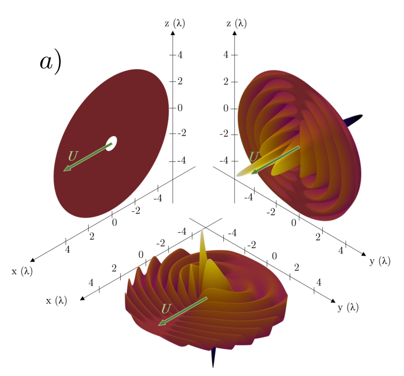
Figure 3: Normalized pressure field created by a dipolar source aligned along y-axis and translating along x-axis calculated with equation (19) represented in (a) the (O,x,z) plane, (b) the (O,y,z) plane and (c) the (O,x,y) plane. To magnify the asymmetry induced by Doppler effect, the pressure field is plotted for a Mach number $M=0.5$.

This pressure field for a translating dipole is represented on figure 3 in the 3 orthogonal planes $(O,x,y)$, $(O,x,z)$ and $(O,y,z)$ for a dipole aligned with $y$ axis (i.e. for $c_{x}=c_{z}=0$ and $c_{y}=1$). In this representation, the Mach number was set to 0.5 to magnify the asymmetry induced by Doppler effect (visible on figure 3.c).

5.2.3 Density field

The density $\rho_{1}$ is simply equal to:

$$\boxed{\rho_{1}=p_{1}/c^{2}}$$ (20)

5.3 Expression of the derivative of the dipolar source

We can see that the time derivative of the force $\mathbf{f^{\prime}}(t)$ appears in all these expressions, which according to equation (2) is equal to:

$$\mathbf{f^{\prime}}(t)\quad=\quad\begin{pmatrix}f^{\prime}_{x}\\ f^{\prime}_{y}\\ f^{\prime}_{z}\end{pmatrix}\quad=\quad F\omega\cos(\omega t)\begin{pmatrix}c_{x}\\ c_{y}\\ c_{z}\\ \end{pmatrix},$$ (21)

and whose mean square is equal to:

$$\left<\mathbf{f^{\prime}}^{2}\right>=\frac{F^{2}\omega^{2}}{2}.$$ (22)

6 Radiation force

The last step is to compute integral (14) with the expression of the velocity, pressure and density fields given by equations (18) to (20). The radiation force $\left<\mathbf{F}_{\text{rad}}\right>$ can be decomposed into 4 contributions: the kinetic energy contribution $\left<\mathbf{F_{k}}\right>$, the potential energy contribution $\left<\mathbf{F_{p}}\right>$, the convective contribution $\left<\mathbf{F_{c}}\right>$ and the translation contribution $\left<\mathbf{F_{t}}\right>$:

$$\left<\mathbf{F_{rad}}\right>=\left<\mathbf{F_{k}}\right>-\left<\mathbf{F_{p}}\right>-\left<\mathbf{F_{c}}\right>+\left<\mathbf{F_{t}}\right>,$$ (23)

whose expressions are given by:

$$\left<\mathbf{F_{k}}\right> =\left<\iint_{S_{\infty}}\frac{\rho_{0}}{2}\mathbf{v_{1}}^{2}\mathbf{n}_{\infty}\mathrm{d}S\right>$$ (24a)

$$\left<\mathbf{F_{p}}\right> =\left<\iint_{S_{\infty}}\frac{1}{\rho_{0}c^{2}}\frac{p_{1}^{2}}{2}\mathbf{n}_{\infty}\mathrm{d}S\right>$$ (24b)

$$\left<\mathbf{F_{c}}\right> =\left<\iint_{S_{\infty}}\rho_{0}(\mathbf{v_{1}}\otimes\mathbf{v_{1}})\mathbf{n}_{\infty}\mathrm{d}S\right>$$ (24c)

$$\left<\mathbf{F_{t}}\right> =\left<\iint_{S_{\infty}}(\mathbf{U}\cdot\mathbf{n}_{\infty})\rho_{1}\mathbf{v_{1}}\mathrm{d}S\right>$$ (24d)

6.1 Potential energy term

Let’s start with the potential energy term:

$$\left<\mathbf{F_{p}}\right>=\frac{1}{32\pi^{2}\rho_{0}c^{4}}\int_{\theta^{*}=0}^{\pi}\int_{\phi^{*}=0}^{2\pi}\left<\left(\nabla R\cdot\mathbf{f^{\prime}}\left(t-\frac{R}{c}\right)\right)^{2}\sin\theta^{*}\mathbf{n}_{\infty}\right>\mathrm{d}\theta^{*}\mathrm{d}\phi^{*}.$$ (25)

We have:

$$\left(\nabla R\cdot\mathbf{f^{\prime}}\left(t-\frac{R}{c}\right)\right)^{2}\sin\theta^{*}\mathbf{n}_{\infty} = \left(\begin{pmatrix}\cos\theta^{*}+M\\ \sin\theta^{*}\cos\phi^{*}\\ \sin\theta^{*}\sin\phi^{*}\end{pmatrix}\cdot\begin{pmatrix}f_{x}^{\prime}\\ f_{y}^{\prime}\\ f_{z}^{\prime}\end{pmatrix}\right)^{2}\begin{pmatrix}\cos\theta^{*}\sin\theta^{*}\\ \sin^{2}\theta^{*}\cos\phi^{*}\\ \sin^{2}\theta^{*}\sin\phi^{*}\end{pmatrix},$$

with

$$\left(\begin{pmatrix}\cos\theta^{*}+M\\ \sin\theta^{*}\cos\phi^{*}\\ \sin\theta^{*}\sin\phi^{*}\end{pmatrix}\cdot\begin{pmatrix}f_{x}^{\prime}\\ f_{y}^{\prime}\\ f_{z}^{\prime}\end{pmatrix}\right)^{2} =(\cos\theta^{*}+M)^{2}f_{x}^{\prime 2}+\sin^{2}\theta^{*}\cos^{2}\phi^{*}f_{y}^{\prime 2}+\sin^{2}\theta^{*}\sin^{2}\phi^{*}f_{z}^{\prime 2}$$

$$+2(\cos\theta^{*}+M)\sin\theta^{*}\cos\phi^{*}f_{x}^{\prime}f_{y}^{\prime}$$

$$+2(\cos\theta^{*}+M)\sin\theta^{*}\sin\phi^{*}f_{x}^{\prime}f_{z}^{\prime}$$

$$+2\sin\theta^{*}\sin\theta^{*}\cos\phi^{*}\sin\phi^{*}f_{y}^{\prime}f_{z}^{\prime}.$$

Let’s take a closer look at $<f_{i}^{\prime}f_{j}^{\prime}>$, with $i$ and $j$ two indexes taken among $\{x,y,z\}$. From equation (21), we can write:

$$<f_{i}^{\prime}f_{j}^{\prime}> = F^{2}\omega^{2}\left<\cos^{2}\left(\omega\left(t-\frac{R}{c}\right)\right)\right>c_{i}c_{j}$$

$$= \frac{F^{2}\omega^{2}}{2}\left<\cos(\psi_{i}-\psi_{j})+\cos\left(2\omega t-2\omega\frac{1+M\cos\theta^{*}}{c}r_{\infty}+\phi_{i}+\phi_{j}\right)\right>c_{i}c_{j}$$

$$= \frac{F^{2}\omega^{2}}{2}c_{i}c_{j}.$$

Hence, within the approximation of small velocity perturbation, we see that $<f_{i}^{\prime}f_{j}^{\prime}>$ does not depend on $\theta^{*}$; we can therefore take these terms out of the integral. Then, the terms in $\cos\phi^{*}$, $\sin\phi^{*}$, and $\cos\phi^{*}\sin\phi^{*}$ cancel when they are integrated over $[0,2\pi]$, as well as the ones in $\cos^{3}\theta^{*}\sin\theta^{*}$, $\cos\theta^{*}\sin^{3}\theta^{*}$, $\cos\theta^{*}\sin\theta^{*}$, and $\cos^{3}\theta^{*}\sin^{3}\theta^{*}$ when they are integrated over $[0,\pi]$. These simplifications lead to:

$$\boxed{\left<\mathbf{F_{p}}\right>=\frac{MF^{2}\omega^{2}}{24\pi\rho_{0}c^{4}}\begin{pmatrix}c_{x}^{2}\\ c_{x}c_{y}\\ c_{x}c_{z}\end{pmatrix}.}$$ (26)

6.2 Kinetic energy term

Now let’s focus on the kinetic energy term:

$$\left<\mathbf{F_{k}}\right>=\int_{\theta^{*}=0}^{\pi}\int_{\phi^{*}=0}^{2\pi}\left<\frac{\rho_{0}}{2}\mathbf{v_{1}}^{2}\mathbf{n}_{\infty}r_{\infty}^{2}\sin\theta^{*}\right>\mathrm{d}\phi^{*}\mathrm{d}\theta^{*}.$$ (27)

We have:

$$\left<\frac{\rho_{0}}{2}\mathbf{v_{1}}^{2}\mathbf{n}_{\infty}r_{\infty}^{2}\sin\theta^{*}\right>=\frac{(1+M\cos\theta^{*})^{2}}{32\pi^{2}c^{4}\rho_{0}}\left<\mathbf{f^{\prime}}^{2}\right>\cdot\begin{pmatrix}\cos\theta^{*}\sin\theta^{*}\\ \sin^{2}\theta^{*}\cos\phi^{*}\\ \sin^{2}\theta^{*}\sin\phi^{*}\end{pmatrix},\\$$ (28)

which with the help of equation (22) turns into:

$$\left<\frac{\rho_{0}}{2}\mathbf{v_{1}}^{2}\mathbf{n}_{\infty}r_{\infty}^{2}\sin\theta^{*}\right>=\frac{(1+M\cos\theta^{*})^{2}}{32\pi^{2}c^{4}\rho_{0}}\frac{F^{2}\omega^{2}}{2}\cdot\begin{pmatrix}\cos\theta^{*}\sin\theta^{*}\\ \sin^{2}\theta^{*}\cos\phi^{*}\\ \sin^{2}\theta^{*}\sin\phi^{*}\end{pmatrix}.$$ (29)

After integration over $\phi*$ and $\theta^{*}$, we get :

$$\boxed{\mathbf{F_{k}}=\frac{MF^{2}\omega^{2}}{24\pi c^{4}\rho_{0}}\mathbf{x}.}$$ (30)

6.3 Convective term

We then study:

$$\left<\mathbf{F_{c}}\right>=\left<\iint_{S_{\infty}}\rho_{0}(\mathbf{v_{1}}\otimes\mathbf{v_{1}})\mathbf{n}_{\infty}\mathrm{d}S\right>.$$

We have :

$$\rho_{0}r_{\infty}^{2}\sin\theta^{*}(\mathbf{v_{1}}\otimes\mathbf{v_{1}})\mathbf{n}_{\infty}=\frac{(1+M\cos\theta^{*})^{2}}{16\pi^{2}c^{4}\rho_{0}}\begin{pmatrix}f_{x}^{\prime 2}&f^{\prime}_{x}f^{\prime}_{y}&f^{\prime}_{x}f^{\prime}_{z}\\ f^{\prime}_{y}f^{\prime}_{x}&f_{y}^{\prime 2}&f^{\prime}_{y}f^{\prime}_{z}\\ f^{\prime}_{z}f^{\prime}_{x}&f^{\prime}_{z}f^{\prime}_{y}&f_{z}^{\prime 2}\end{pmatrix}\begin{pmatrix}\cos\theta^{*}\sin\theta^{*}\\ \sin^{2}\theta^{*}\cos\phi^{*}\\ \sin^{2}\theta^{*}\sin\phi^{*}\end{pmatrix}.$$

When integrating over $\phi^{*}$, we find that the terms in $\cos\phi^{*}$ and $\sin\phi^{*}$ cancel so that:

$$\left<\mathbf{F_{c}}\right> = 2\pi\int_{0}^{\pi}\left<\frac{(1+M\cos\theta^{*})^{2}}{16\pi^{2}c^{4}\rho_{0}}\cos\theta^{*}\sin\theta^{*}\begin{pmatrix}f_{x}^{\prime 2}\\ f^{\prime}_{y}f^{\prime}_{x}\\ f^{\prime}_{z}f^{\prime}_{x}\end{pmatrix}\right>\mathrm{d}\theta^{*}$$

$$= \frac{F^{2}\omega^{2}}{16\pi c^{4}\rho_{0}}\begin{pmatrix}c_{x}^{2}\\ c_{y}c_{x}\\ c_{z}c_{x}\end{pmatrix}\int_{0}^{\pi}(1+2M\cos\theta^{*})\cos\theta^{*}\sin\theta^{*}\mathrm{d}\theta^{*}$$

$$= \frac{MF^{2}\omega^{2}}{16\pi c^{4}\rho_{0}}\begin{pmatrix}c_{x}^{2}\\ \alpha_{yx}c_{y}c_{x}\\ \alpha_{zx}c_{z}c_{x}\end{pmatrix}\times\frac{4}{3}.$$

Finally, we obtain:

$$\boxed{\mathbf{F_{c}}=\frac{MF^{2}\omega^{2}}{12\pi c^{4}\rho_{0}}\begin{pmatrix}c_{x}^{2}\\ c_{y}c_{x}\\ c_{z}c_{x}\end{pmatrix}.}$$ (31)

6.4 Source translation term

And finally we can compute the translation term:

$$\left<\mathbf{F_{t}}\right>=\left<\iint_{S_{\infty}}(\mathbf{U}\cdot\mathbf{n}_{\infty})\rho_{1}\mathbf{v_{1}}\mathrm{d}S\right>.$$

We have:

$$(\mathbf{U}\cdot\mathbf{n}_{\infty})\rho_{1}\mathbf{v_{1}}r_{\infty}^{2}\sin\theta^{*} = Mc\;\mathbf{x}\cdot\begin{pmatrix}\cos\theta^{*}\sin\theta^{*}\\ \sin^{2}\theta^{*}\cos\phi^{*}\\ \sin^{2}\theta^{*}\sin\phi^{*}\end{pmatrix}\frac{p_{1}}{c^{2}}\mathbf{v_{1}}r_{\infty}^{2}$$

$$= M\cos\theta^{*}\sin\theta^{*}\frac{1+M\cos\theta^{*}}{16\pi^{2}c^{4}\rho_{0}}\left[\begin{pmatrix}\cos\theta^{*}+M\\ \sin\theta^{*}\cos\phi^{*}\\ \sin\theta^{*}\sin\phi^{*}\end{pmatrix}\cdot\begin{pmatrix}f^{\prime}_{x}\\ f^{\prime}_{y}\\ f^{\prime}_{z}\end{pmatrix}\right]\begin{pmatrix}f^{\prime}_{x}\\ f^{\prime}_{y}\\ f^{\prime}_{z}\end{pmatrix}.$$

As previously, the terms in $\sin\phi^{*}$ and $\cos\phi^{*}$ cancel when integrating, leading to:

$$\left<\mathbf{F_{t}}\right> = \int_{0}^{\pi}M\cos\theta^{*}\sin\theta^{*}\frac{1+M\cos\theta^{*}}{8\pi c^{4}\rho_{0}}(\cos\theta^{*}+M)\left<\begin{pmatrix}f^{\prime}_{x}f^{\prime}_{x}\\ f^{\prime}_{x}f^{\prime}_{y}\\ f^{\prime}_{x}f^{\prime}_{z}\end{pmatrix}\right>\mathrm{d}\theta^{*}$$

$$= \frac{MF^{2}\omega^{2}}{16\pi c^{4}\rho_{0}}\int_{0}^{\pi}\cos\theta^{*}\sin\theta^{*}(1+M\cos\theta^{*})(\cos\theta^{*}+M)\begin{pmatrix}c_{x}^{2}\\ c_{x}c_{y}\\ c_{x}c_{z}\end{pmatrix}\mathrm{d}\theta^{*}$$

$$= \frac{MF^{2}\omega^{2}}{16\pi c^{4}\rho_{0}}\begin{pmatrix}c_{x}^{2}\\ c_{x}c_{y}\\ c_{x}c_{z}\end{pmatrix}\times\frac{2}{3}.$$

We finally obtain:

$$\boxed{\left<\mathbf{F_{t}}\right>=\frac{MF^{2}\omega^{2}}{24\pi c^{4}\rho_{0}}\begin{pmatrix}c_{x}^{2}\\ c_{x}c_{y}\\ c_{x}c_{z}\end{pmatrix}.}$$ (32)

6.5 Total radiation force

If we now gather equations (30) to (32), we obtain:

$$\left<\mathbf{F_{rad}}\right> = \left<\mathbf{F_{k}}\right>-\left<\mathbf{F_{p}}\right>-\left<\mathbf{F_{c}}\right>+\left<\mathbf{F_{t}}\right>$$

$$= \frac{MF^{2}\omega^{2}}{24\pi c^{4}\rho_{0}}\mathbf{x}+\begin{pmatrix}c_{x}^{2}\\ c_{x}c_{y}\\ c_{x}c_{z}\end{pmatrix}\left(-\frac{MF^{2}\omega^{2}}{24\pi\rho_{0}c^{4}}-\frac{MF^{2}\omega^{2}}{12\pi c^{4}\rho_{0}}+\frac{MF^{2}\omega^{2}}{24\pi c^{4}\rho_{0}}\right),$$

and thus the final expression of the self-induced radiation force acting on a translating dipolar source:

$$\boxed{\left<\mathbf{F_{rad}}\right>=\frac{MF^{2}\omega^{2}}{12\pi c^{4}\rho_{0}}\begin{pmatrix}1/2-c_{x}^{2}\\ -c_{x}c_{y}\\ -c_{x}c_{z}\end{pmatrix}.}$$ (33)

7 Discussion

As expected, this expression shows that the radiation force only exists in presence of a velocity perturbation i.e. for $U=Mc\neq 0$ and the radiation force is proportional to the intensity of the wave radiated by the source. An interesting point is that the projection of this radiation force along the velocity perturbation axis $\mathbf{x}$ can be either positive or negative depending on the orientation of the dipole. To further analyse this expression, it is interesting to introduce the spherical coordinates ($\hat{\theta}$, $\hat{\phi}$) of the unit vector $\mathbf{c}$ which sets the direction of the dipolar radiation:

$$c_{x}=\cos\hat{\theta},$$ (34a)

$$c_{y}=\sin\hat{\theta}\cos\hat{\phi},$$ (34b)

$$c_{z}=\sin\hat{\theta}\sin\hat{\phi}.$$ (34c)

If we replace these expressions in (33), and compute the norm of the radiation force, we obtain:

$$\|\left<\mathbf{F}_{\text{rad}}\right>\| = \frac{MF^{2}\omega^{2}}{12\pi c^{4}\rho_{0}}\sqrt{\left(\frac{1}{2}-\cos^{2}\hat{\theta}\right)^{2}+\cos^{2}\hat{\theta}\sin^{2}\hat{\theta}\cos^{2}\hat{\phi}+\cos^{2}\hat{\theta}\sin^{2}\hat{\theta}\sin^{2}\hat{\phi}}$$ (35)

$$= \frac{MF^{2}\omega^{2}}{12\pi c^{4}\rho_{0}}\sqrt{\frac{1}{4}-\cos^{2}\hat{\theta}+\cos^{4}\hat{\theta}+\cos^{2}\hat{\theta}\sin^{2}\hat{\theta}}$$

$$= \frac{MF^{2}\omega^{2}}{12\pi c^{4}\rho_{0}}\sqrt{\frac{1}{4}+\cos^{2}\hat{\theta}\left(-1+\cos^{2}\hat{\theta}+\sin^{2}\hat{\theta}\right)}$$

$$= \frac{MF^{2}\omega^{2}}{24\pi c^{4}\rho_{0}}.$$

This calculation shows that the radiation force magnitude is independent of the angles ($\hat{\theta}$, $\hat{\phi}$) between the dipole orientation and the perturbation displacement.

Let’s now consider the above calculation as a stability analysis, with a stable state corresponding to the dipolar source at rest perturbed by a small velocity perturbation. Then the most unstable situation arises when the projection of the force along the velocity perturbation $\mathbf{x}$ is maximum, since in this case the amplification of the velocity perturbation by the radiation force will be maximum. Since the magnitude of the radiation force is constant whatever the orientation of the dipole, this happens when $\left<\mathbf{F}_{\text{rad}}\right>$ is directed in the $\mathbf{x}$ direction, i.e. when $\hat{\theta}=\frac{\pi}{2}$. The same result is of course obtained if we maximize $\left<\mathbf{F}_{\text{rad}}\right>.\mathbf{x}=\frac{1}{2}-\cos^{2}\hat{\theta}$. Since the most unstable situations correspond to a dipole direction orthogonal displacement, an interesting point is that the direction of motion is not set a priori by the anisotropy of the source as in recent experiments with capillary and gravity waves ([Ho et al.(2021), Benham et al.(2022)]) surfers.

8 Conclusion and perspectives

In this paper, we compute the self-radiation force exerted on a dipolar source in presence of a small axial velocity perturbation. We show that when the dipole orientation is orthogonal to the velocity perturbation axis, the radiation force is aligned with the motion hence amplifying it. This result suggests the possibility of an acoustical source surfing on its own acoustic field, a prerequisite for pilot waves analogues. From a theoretical point of view, a next step would be to derive constitutive equations for these acoustic surfers dynamics. It would also be interesting to investigate the response of an arbitrary multipole source since our result with monopolar and dipolar sources exhibit drastically different behaviours. Of course the most compelling challenge would be to materialize these acoustic surfers experimentally. Many different types of acoustic sources and surrounding fluids can be envisionned. A first requirement is to find a way to excite these acoustic surfers in absence of any incident directional acoustic field. Otherwise the source will be driven by this incident field and not by its own wave. Different possibilities can be considered as (i) using a non-acoustic homogeneous field to excite the source (acceleration, magnetic, electric) or (ii) creating a stochastic acoustic field which does not prescribe the motion in any specific direction. A second requirement is that the radiation force should overcome the drag force for the situation to be unstable. This might require to work in low viscosity fluids, such as gases, cryogenic fluids or superfluids.

This work hence paves the way for further theoretical, numerical and experimental investigation of acoustic quantum analogues.

Declaration of Interests

The authors report no conflict of interest.

References

• [Andersen et al.(2015)] Andersen, A., Madsen, J., Reichelt, C., Ahl, S.R. & Lautrup, B. 2015 Double-slit exper- iment with single wave-driven particles and its relation to quantum mechanics. Phys. Rev. E 92, 013006.
• [Baresch et al.(2013)] Baresch, Diego, Thomas, Jean-Louis & Marchiano, Régis 2013 Three-dimensional acoustic radiation force on an arbitrarily located elastic sphere. J. Acoust. Soc. Am. 133 (1), 25–36.
• [Baresch et al.(2016)] Baresch, D., Thomas, J.-L. & Marchiano, R. 2016 Observation of a single-beam gradient force acoustical trap for elastic particles: acoustical tweezers. Phys. Rev. lett. 116 (2), 024301.
• [Baudoin et al.(2019)] Baudoin, M., Gerbedoen, J.-C., Riaud, A., Bou Matar, O., Smagin, N. & Thomas, J.-L. 2019 Folding a focalized acoustical vortex on a flat holographic transducer: miniaturized selective acoustical tweezers. Sci. Adv. 5, eaav1967.
• [Baudoin & Thomas(2020)] Baudoin, M. & Thomas, J.-L. 2020 Acoustic tweezers for particle and fluid micromanipulation. Annu. Rev. Fluid Mech. 52, 205–234.
• [Baudoin et al.(2020)] Baudoin, M., Thomas, J.-L., Sahely, R. Al, Gerbedoen, J.-C., Gong, Z., Sivery, A., Bou Matar, O., Smagin, N., Favreau, P. & Vlandas, A. 2020 Spatially selective manipulation of cells with single-beam acoustical tweezers. Nat. Commu. 11, 4244.
• [Benham et al.(2022)] Benham, G.P., Devauchelle, O., Morris, S.W. & Neufeld, J.A. 2022 Gunwale bobbing. Phys. Rev. Fluids 7, 074804.
• [Biquard(1932a)] Biquard, P. 1932a Les ondes ultra-sonores. Rev. D’Acous. 1, 93–109.
• [Biquard(1932b)] Biquard, P. 1932b Les ondes ultra-sonores ii. Rev. D’Acous. 1, 315–355.
• [Brillouin(1925)] Brillouin, L. 1925 Les tensions de radiation; leur interprétation en mécanique classique et en relativité. J. Phys. Radium 6, 337–353.
• [Bush & Oza(2020)] Bush, J.W.M. & Oza, A.U. 2020 Hydrodynamic quantum analogs. Rep. Prog. Phys. 84, 017001.
• [Couder & Fort(2006)] Couder, Y. & Fort, E. 2006 Single-particle diffraction and interference at a macroscopic scale. Phys. Rev. Lett. 97, 154101.
• [Couder et al.(2005)] Couder, Y., Protiere, S., Fort, E. & Boudaoud, A. 2005 Walking and orbiting droplets. Nature 437, 208.
• [Cristea-Platon et al.(2018)] Cristea-Platon, T., Sáenz, P.J. & Bush, J.W.M. 2018 Walking droplets in a circular corral: quantisation and chaos. Chaos 28, 096116.
• [Dubertrand et al.(2016)] Dubertrand, R., Hubert, M., Schlagheck, P., Vandewalle, N., Bastin, T. & Martin, J. 2016 Scattering theory of walking droplets in the presence of obstacles. New J. Phys. 18, 113037.
• [Eddi et al.(2009)] Eddi, A., Fort, E., Moisy, F. & Couder, Y. 2009 Unpredictable tunneling of a classical wave–particle association. Phys. Rev. Lett. 102, 240401.
• [Ellegaard & Levinsen(2020)] Ellegaard, C. & Levinsen, M.T. 2020 Interaction of wave-driven particles with slit structures. Phys. Rev. E 102, 023115.
• [Faraday(2022)] Faraday, M. 2022 On the forms and states assumed by fluids in contact with vibrating elastic surface. Phil. Tran. R. Soc. Lond. 121, 319.
• [Faria(2017)] Faria, L.M. 2017 A model for Faraday pilot waves over variable topography. J. Fluid Mech. 811, 51–66.
• [Fort et al.(2010)] Fort, E., Eddi, A., Boudaoud, A., Moukhtar, J. & Couder, Y. 2010 Path-memory induced quantization of classical orbits. Proc. Natl Acad. Sci. USA 107, 17515.
• [Gilet(2014)] Gilet, T. 2014 Dynamics and statistics of wave-particle interactions in a confined geometry. Phys. Rev. E 90, 052917.
• [Gilet(2016)] Gilet, T. 2016 Quantumlike statistics of deterministic wave–particle interactions in a circular cavity. 2016 93, 042202.
• [Gong & Baudoin(2020)] Gong, Z. & Baudoin, M. 2020 Radiation torque on a particle in a fluid: an angular spectrum based compact expression. J. Acoust. Soc. Am. 148 (5), 3131–3140.
• [Gong & Baudoin(2021)] Gong, Z. & Baudoin, M. 2021 Equivalence between angular spectrum-based and multipole expansion-based formulas of the acoustic radiation force and torque. J. Acoust. Soc. Am. 149 (5), 3469–3482.
• [Harris & Bush(2014)] Harris, D.M. & Bush, J.W.M. 2014 Droplets walking in a rotating frame: from quantized orbits to multimodal statistics. J. Fluid Mech. 739, 444.
• [Harris et al.(2013)] Harris, D.M., Moukhtar, J., Fort, E., Couder, Y. & Bush, J.W.M. 2013 Wavelike statistics from pilot-wave dynamics in a circular corral. Phys. Rev. E 88, 011001.
• [Ho et al.(2021)] Ho, I., Pucci, G., Oza, A.U. & Harris, D.M. 2021 Capillary surfers: wave driven particles at a fluid interface. arXiv p. 102.11694.
• [Hubert et al.(2017)] Hubert, M., Labousse, M. & Perrard, S. 2017 Self-propusion and crossing statistics under random initial conditions. Phys. Rev. E 95, 062507.
• [Kumar & Tuckerman(1994)] Kumar, K. & Tuckerman, L.S. 1994 Parameteric instability of the interface between two fluids. J. Fluid Mech. 279, 49–68.
• [Marzo et al.(2015)] Marzo, A., Seah, S.A., Drinkwater, B.W., Sahoo, D.R., Long, B. & Subramanian, S. 2015 Holographic acoustic elements for manipulation of levitated objects. Nat. Commu. 6, 8661.
• [Morse & Ingard(1968)] Morse, P.M. & Ingard, K.U. 1968 Theoretical acoustics. New York: McGraw-Hill book company.
• [Nachbin et al.(2017)] Nachbin, A., Milewski, P.A. & Bush, J.W.M. 2017 Tunneling with a hydrodynamic pilot-wave model. Phys. Rev. Fluids 2, 034801.
• [Oza et al.(2014)] Oza, A.U., Harris, D.M., Rosales, R.R. & Bush, J.W.M. 2014 Pilot-wave dynamics in a rotating frame: on the emergence of orbital quantization. J. Fluid Mech. 744, 404.
• [Pucci et al.(2018)] Pucci, G., Harris, D.M., Faria, L.M. & Bush, J.W.M. 2018 Walking droplets interacting with single and double slits. J. Fluid Mech. 835, 1136–56.
• [Rayleigh(1905)] Rayleigh, J.W.S. 1905 On the momentum and pressure of gaseous vibrations, and on the connection with the virial theorem. Philos. Mag. 10, 366–374.
• [Riaud et al.(2017)] Riaud, A., Baudoin, M., Bou Matar, O., Becerra, L. & Thomas, J.-L. 2017 Selective manipulation of microscopic particles with precursor swirling Rayleigh waves. Phys. Rev. Applied 7, 024007.
• [Rode et al.(2019)] Rode, M., Madsen, J. & Andersen, A. 2019 Wave fields in double-slit experiments with wave-driven droplets. Phys. Rev. Fluids 4, 104801.
• [Roux et al.(2022)] Roux, A., Martischang, J.-P. & Baudoin, M. 2022 Self-radiation force on a moving monopolar source. Journal of Fluid Mechanics 952, A22.
• [Rufo et al.(2022)] Rufo, J., Cai, F., Friend, J., Wiklund, M. & Huang, T.J. 2022 Acoustofluidics for biomedical applications. Nat. Rev. Meth. Prim. 2, 30.
• [Sapozhnikov & Bailey(2013)] Sapozhnikov, Oleg A & Bailey, Michael R 2013 Radiation force of an arbitrary acoustic beam on an elastic sphere in a fluid. J. Acoust. Soc. Am. 133 (2), 661–676.
• [Silva et al.(2012)] Silva, GT, Lobo, TP & Mitri, FG 2012 Radiation torque produced by an arbitrary acoustic wave. EPL (Europhysics Letters) 97 (5), 54003.
• [Silva(2011)] Silva, Glauber T 2011 An expression for the radiation force exerted by an acoustic beam with arbitrary wavefront (l). J. Acoust. Soc. Am. 130 (6), 3541–3544.
• [Sáenz et al.(2020)] Sáenz, P.J., Cristea-Platon, T. & Bush, J.W.M. 2020 A hydrodynamic analog of Friedel oscillations. Sci. Adv. 6, 20.
• [Sáenz et al.(2018)] Sáenz, P. J., Cristea-Platon, T. & Bush, J.W.M. 2018 Statistical projection effects in a hydrodynamic pilot-wave system. Nat. Phys. 14, 315.
• [Tadrist et al.(2020)] Tadrist, L., Gilet, T., Schlagheck, P. & Bush, J.W.M. 2020 Predictability in a hydrodynamic pilot-wave system: resolution of walker tunneling. Phys. Rev. E 102, 013104.