A generalization of Floater–Hormann interpolants
Abstract
In this paper the interpolating rational functions introduced by Floater and Hormann are generalized leading to a whole new family of rational functions depending on , an additional positive integer parameter. For , the original Floater–Hormann interpolants are obtained. When we prove that the new rational functions share a lot of the nice properties of the original Floater–Hormann functions. Indeed, for any configuration of nodes in a compact interval, they have no real poles, interpolate the given data, preserve the polynomials up to a certain fixed degree, and have a barycentric-type representation. Moreover, we estimate the associated Lebesgue constants in terms of the minimum () and maximum () distance between two consecutive nodes. It turns out that, in contrast to the original Floater-Hormann interpolants, for all we get uniformly bounded Lebesgue constants in the case of equidistant and quasi-equidistant nodes configurations (i.e., when ). For such configurations, as the number of nodes tends to infinity, we prove that the new interpolants () uniformly converge to the interpolated function , for any continuous function and all . The same is not ensured by the original FH interpolants (). Moreover, we provide uniform and pointwise estimates of the approximation error for functions having different degrees of smoothness. Numerical experiments illustrate the theoretical results and show a better error profile for less smooth functions compared to the original Floater-Hormann interpolants.
1 Introduction
In this paper, we consider the problem of interpolating a function on a finite interval , given its values in nodes . Without loss of generality the interval can be taken. If one can choose the position of the nodes in the interval, an analytic function can be approximated by polynomials interpolating at the Chebyshev points of the first or second kind, leading to exponential convergence. The speed of convergence is determined by the largest Bernstein ellipse that can be taken in the analytic domain of the function. For differentiable functions, the convergence is algebraic where the speed of convergence is determined by the smoothness of the function. For further details we refer the reader to the book of Trefethen [14].
If the nodes can not be freely chosen, the problem becomes much harder. E.g., when the nodes are equidistant in the interval and we want to approximate the function , the Runge phenomenon occurs and the approximation error becomes very large in the neighborhood of the endpoints of the interval when the number of nodes increases. In [12] Huybrechs and Trefethen compare several methods to approximate a function when the nodes are equidistant. One of these methods uses the Floater–Hormann (briefly FH) interpolating rational functions [8]. This method is valid for any configuration of the nodes but turns out to be very useful for equidistant configurations. Generalizing [1], Floater and Hormann introduced a blended form of interpolating polynomials of fixed degree , leading to the rational function [8]
| (1) |
where, for all ,
| (2) |
and denotes the unique polynomial of degree interpolating at the points .
Note that in the limit case , we get , , and (1) yields the Berrut rational interpolants studied in [1]. By taking any , Floater and Hormann proved that the approximant has no poles on the real line, it coincides with on the set of nodes , and, at any , it admits a barycentric representation allowing efficient and stable computations [5]. Moreover, for any fixed , as (and hence ), regardless of the distribution of nodes, the FH approximation error behaves as follows [8, Thm. 2]
| (3) |
where, as usual, .
Therefore the FH interpolants, which for reduce to Berrut interpolants [8], are able to produce arbitrarily high approximation orders provided that the parameter is large enough. However, in the important case of equidistant or quasi–equidistant nodes, it has been proved that the Lebesgue constants of FH interpolants grow logarithmically with , but exponentially with [4, 10]. Hence, increasing too much is not always advisable.
For an overview of linear barycentric rational interpolation, we refer the interested reader to the paper of Berrut and Klein [2]. This overview also describes a generalization of the FH interpolant developed by Klein [13] in the case of equidistant nodes. See also [6, 7].
In this paper we are also going to generalize the method of Floater and Hormann but in a different way. For any distribution of nodes, we define a whole family of linear rational approximants that are denoted by and depend, besides , on an additional parameter . When , reduces to the original FH interpolant . When and , reduces to the approximants studied in [15]. In this paper, for brevity, we only consider the case of arbitrary , the case will be investigated in future work.
Similarly to the original FH interpolants , we show that, for all , also has no real poles, interpolates the data, and has a barycentric type representation. However, the main results of the paper concern the case of equidistant or quasi-equidistant configurations of nodes, where we find some novelty by taking . First of all, we prove that
| (4) |
which is not ensured when . Moreover, in contrast to the original FH interpolants, we prove that for equidistant or quasi-equidistant nodes, the Lebesgue constants corresponding to any and are uniformly bounded both in and , but still grow exponentially with .
With respect to the approximation rate, for equidistant or quasi-equidistant nodes, we show that
| (5) |
holds as , for arbitrarily fixed parameters and . Hence, generalized FH interpolants also provide arbitrarily high convergence rates. Moreover, making the comparison with (3), if we take in (5) then we get that the generalized FH functions , with parameter , also can reach the convergence order but supposing that instead of .
In addition, we estimate the error of generalized FH interpolants also for functions with a non-integer smoothness degree. More precisely, in the class of Hölder continuous functions with exponent , we prove that
| (6) |
Moreover, in the class of functions that are -times continuously differentiable and have the –th derivative Hölder continuous with exponent , the generalized FH function corresponding to any satisfies
| (7) |
for all integers .
Finally, we consider the pointwise error and show that, even in the case of almost everywhere continuous functions with some isolated discontinuities, the approximation orders displayed in (5)–(7) are locally preserved and continue to hold in all compact subintervals where has the described smoothness degree (i.e., , , and , resp.)
The numerical experiments confirm the theoretical estimates and show that less restrictive assumptions on could be possible for getting the previous error trend. Moreover, in comparison with the original FH interpolants, the generalized ones exhibit a much better error profile when the interpolated function is less smooth.
The paper is organized as follows. In Section 2 the generalized FH rational interpolants are presented. In Section 3 we state and prove several properties of these new interpolants which are similar to those of the original FH interpolants. In Section 4 we focus on the case of equidistant or quasi-equidistant nodes and estimate the behaviour of the associated Lebesgue constants. This section concludes with two subsections: in the former the proof and the necessary technical lemmas are given, in the latter a useful related result is stated. In Section 5 the convergence theorem and all the error estimates are given. In Section 6 we illustrate several numerical examples comparing generalized and original FH approximants. Finally, Section 7 gives the conclusion of our paper.
2 Generalized Floater–Hormann interpolants
Let
| (8) |
be any sequence of nodes where we assume the function has been sampled. The generalized FH approximation of is defined very similarly to (1) and (2). For any integer , it is also a blended form of the polynomial interpolants of degree at most . However, the blending functions depend on an additional parameter and are defined as follows
| (9) |
Hence, for arbitrarily fixed and , the generalized FH approximation of is given by
| (10) |
where is defined in (9) and is the polynomial of degree interpolating at the nodes .
We point out that the function depends on , on , on the nodes (8), and on two integer parameters: and . Sometimes we also use the notation and in order to highlight the dependence on and .
Note that the original FH interpolants are a special case of the generalized ones with parameter (compare (2) and (9)).
If we multiply both the numerator and denominator of (10) by the polynomial
| (11) |
then we get
| (12) |
where we set
| (13) |
being understood that whenever the product is empty, i.e., if .
Equation (12) yields the generalized FH approximant as a quotient of two polynomials
| (14) |
where the maximum degree is at the numerator and at the denominator, i.e., for all , is a rational function of type .
3 Properties
In this section, we are going to prove that, for any choice of the integer parameter , the generalized FH function has similar properties to the original .
3.1 No poles on the real line
In the case the polynomials defined in (13) were investigated by Floater and Hormann in [8, Thm. 1]. Using their result, the following lemma can be easily deduced:
Lemma 3.1
Let , , and be arbitrarily fixed.
For any that is even, and , we have
| (15) |
If is odd, we distinguish the following cases:
-
•
In the case we have
(16) -
•
In the case , if for any , then we have the following
-
(A)
If then
-
(B)
Suppose , for , the sequence has alternate signs, ending with , and it has increasing absolute values, i.e.,
(17) -
(C)
For , the sequence has alternate signs, starting with , and it has decreasing absolute values, i.e.,
(18)
-
(A)
-
•
In the case , the sequence , for , has alternate sign, starting with , and it has decreasing absolute values, i.e.,
(19) -
•
In the case , the sequence , for , has alternate sign, ending with , and it has increasing absolute values, i.e.,
(20)
From the previous lemma we deduce the following result that generalizes [8, Thm. 1].
Theorem 3.2
For all integers and , the generalized FH rational function has no real poles.
Proof of Theorem 3.2
Recalling (12), it is sufficient to prove that
| (21) |
This follows from (15) in the case that is even. If is odd, by (16) we get
in the case that is odd, and
when is even. Hence, it remains to prove (21) only in the case that is odd and for some . In such a case, we write
being understood that in case of empty summation, i.e., if .
Finally, we observe that whenever the previous summation are non empty, they are positive by virtue of Lemma 3.1 (cf. (A)–(C)). Since at least one term of the summation is not empty, we have proven the theorem.
3.2 Interpolation of the data
In the case it is known that the FH rational function is equal to if is one of the nodes (8). Such interpolation property remains valid for the generalized FH approximation.
Theorem 3.4
For all and any integer , we have
| (25) |
3.3 Preservation of polynomials
Similarly to the classical FH interpolants, also the generalized ones reduce to the identity on the set of all polynomials of degree at most .
3.4 Barycentric-type representation
We recall that the classical FH interpolants are rational functions of type , hence they can be expressed in barycentric form. In this subsection, we give a barycentric-type expression for the generalized FH interpolants defined by (10) and (9), for any parameter .
The Lagrange representation for the interpolating polynomial is
Combining this with (9), we get
Hence, we obtain
and changing the order of the summations, we get
where we recall has been introduced in (26).
Hence, defining
| (28) |
we can write
| (29) |
Similarly, we obtain
| (30) |
that is (29) in the case of the unit function , .
In conclusion, the generalized FH interpolant (10) can be expressed in the following barycentric-type form
| (31) |
Note that in the case , this yields the classical barycentric form
| (32) |
where the weights can be computed in advance and where, in the denominators, we have a factor instead of .
Note that for the weights can not be precomputed. Hence, to evaluate the new interpolant, in -values FLOPS are needed while for the classical barycentric form the weights can be computed beforehand using (32) in FLOPS. Using a more complicated pyramid algorithm [11], this can even be reduced to FLOPS. Evaluating the classical barycentric form in -values costs an additional FLOPS. Hence, it is more efficient to evaluate the classical FH interpolant in comparison to the new one. However, the new approximant exhibits better performance with respect to the error, especially for less smooth functions, as will be shown in the numerical examples.
4 Lebesgue constants
Set for brevity
| (33) |
i.e., defining
| (34) |
we can write
| (35) |
The Lebesgue constant and function of the generalized FH interpolants at the nodes (8) are given by
Their behaviour as is an important measure for the conditioning of the problem, being well–known that
Moreover, using the polynomial reproducing property (27), it is easy to prove that the Lebesgue constants are also involved in the error estimate
where denotes the error of best approximation of in w.r.t. the uniform norm , namely
| (36) |
For classical FH interpolation () the Lebesgue constants have been estimated in [3, 4] for equidistant nodes and in [10] for quasi–equidistant nodes. In both cases, they result to grow as with and as with . Here we show that, introducing the additional parameter , for the generalized FH interpolation we succeed in getting Lebesgue constants uniformly bounded w.r.t. .
More precisely, setting
| (37) |
we have the following
Theorem 4.1
For all , with and , we have
| (38) |
where is a constant independent of and .
Remark 4.2
Similarly to the classic FH interpolation, we note that the dependence on of the Lebesgue constants is exponential for all too. Indeed, we conjecture the linear factor in (38) can be removed, but we were not able to prove it.
An immediate consequence of Thm. 4.1 is the following
Corollary 4.3
Let , with and . In the case of equidistant nodes (i.e., if ) and, more generally, in the case of quasi–equidistant nodes (i.e., if holds with independent of ), we get
4.1 Proof of Theorem 4.1
In order to prove Thm. 4.1 let us first state three preliminary lemmas
Lemma 4.4
Proof of Lemma 4.4
Firstly note that the following inequality
| (40) |
can be proved by taking into account that
In addition, by (24), we deduce
| (41) |
Lemma 4.5
Let with and . If , with , then for all and any , we have
| (42) |
where is the complementary set of defined in (23).
Proof of Lemma 4.5
Taking into account that
| (43) |
we get
| (44) | |||||
| (45) |
Also, by (43), we have
| (46) | |||||
Hence, the statement follows by applying (44)–(46) to the result of Lemma 4.4.
Lemma 4.6
For all and , with , we have
| (47) |
Proof of Theorem 4.1
First of all, note that if then the statement is trivial since, by (34), we have
Hence, let us assume with , and prove (38).
i.e., set for brevity
| (50) |
we have
| (51) |
Now we note that
where is given by (23) and is the complementary set.
Let us first estimate
by distinguishing the following cases:
-
•
Case . Let us estimate the term
-
•
Case . Let us estimate the term
-
•
Case . Let us estimate the summation of the remaining terms .
Summing up, by (52)–(63) we have proved that satisfies the bound in (38).
Now let us prove that the same holds for
We note that if or then we certainly have . Thus, is, indeed, given by the following sum
Hence, by using Lemma 4.5 and Lemma 4.6, we get
Now we distinguish the following cases:
-
•
If then we have and . Hence we can write
and taking into account that, for , the right hand side term takes its maximum value when , we get
(65) -
•
If then we have
(66) -
•
If then we have
(67) -
•
If then we have and . Hence we can write
and since, for , the maximum value of the right hand side term is achieved when , we get
(68)
Thus, by virtue of (65)–(68), we have proved
Consequently, taking into account that the set has at most elements, the estimate of continues as follows
| (71) | |||||
| (78) | |||||
| (81) |
4.2 A related result
Going along the same lines as the proof of Thm. 4.1, we get the following result which will be useful in the next section.
Theorem 4.7
For all , with and , let be the interpolating basis defined in (34). If the distribution of nodes is such that holds ( meaning that the ratio is between two absolute, positive, constants) then for all we have
| (82) |
where is a constant independent of , bounded with respect to but exponentially growing with .
Proof of Theorem 4.7. Recalling that (cf. (34)), if then the statement is trivial since . Hence, let us fix with . Following the same lines as in the proof of Thm. 4.1 and using the notations therein introduced, we note that
Hence, we estimate and using the results obtained in the proof of Thm. 4.1 for and , respectively.
For simplicity, in the sequel we denote by all positive constants as in the statement, even if they have different values.
As regards , similarly to in the proof of Thm. 4.1, we deduce
having used the hypothesis to get the last inequality.
Now we observe that for all it is
and for all it is
Hence, the following holds
| (85) |
which implies
Finally, as regards , we deduce the following from the results achieved for in the proof of Thm. 4.1
having used to get the last inequality.
5 Error estimates
First of all let us state the following fundamental result
Theorem 5.1
Let the parameters be arbitrarily fixed with . Moreover, let the distribution of nodes satisfy . as . Then for any continuous function we have
| (91) |
Proof of Theorem 5.1. Let us arbitrarily fix with , and consider arbitrarily large integers . First, we prove that (91) holds if is any polynomial. Due to (27), this is trivial if . Hence let be a polynomial of degree
Taking into account that certainly preserves the constant function (since ), by (35) we have
and consequently, for all integers , we get
| (92) |
On the other hand, by the Mean Value Theorem, we note that
| (93) |
In conclusion, by collecting (92) and (93), , we get
and applying Thm. 4.7 we obtain
where is independent of .
Hence, by taking the limit as , we conclude that (91) holds whenever is a polynomial.
Now let us prove it for any .
Corresponding to each , by the Weierstrass Theorem, there exists a polynomial such that
Moreover, since , there exists such that
Finally, note that by applying Thm. 4.1 with , we get
where is independent of .
Summing up, from the above results we conclude that such that we have
that means (91) holds for arbitrary .
In the following, we provide several estimates of the convergence order by supposing different degrees of smoothness for the function .
Let us start by providing an error estimate in the case that is a Hölder continuous function satisfying
| (94) |
with and independent of and .
Denoted by the class of all such functions, we state the following
Theorem 5.2
Let be the generalized FH interpolant corresponding to fixed parameters , , arbitrary large , and a distribution of nodes satisfying . For any , if we have then we get
| (95) |
where is a constant as in Theorem 4.7.
Proof of Theorem 5.2. From (92) and (94) we deduce that
holds for all . Hence, the statement follows by applying Thm. 4.7.
Now, let us estimate the error in the case belongs to the class of all functions that are –times continuously differentiable in .
Theorem 5.3
Let be the generalized FH interpolant corresponding to fixed parameters with , arbitrary large , and a distribution of nodes satisfying . For any integer , if then we have
| (96) |
where is a constant as in Theorem 4.7.
Proof of Theorem 5.3. Due to the interpolation property (25), it is sufficient to prove (96) in the case that is arbitrarily fixed, for any .
Since with , we can certainly consider the Taylor polynomial of centered at and having degree , namely
| (97) |
Recalling the Lagrange form of the remainder term, we get the following error-bound
| (98) |
where here and in the following denotes any constant as in Thm. 4.7 which can take also different values at different occurrences.
Since , we can use the polynomial preservation property (27), that combined with (98) yields
where in the last inequality we used .
On the other hand, since
holds, we have
Thus, we conclude that
We remark that Thm. 5.3 for states that the analogous of (3) holds for generalized FH interpolants too, but under weaker assumption on the function .
Now we estimate the error in the class of all functions that are –times continuously differentiable with , .
Theorem 5.4
Let be the generalized FH interpolant corresponding to fixed parameters with , arbitrary large , and a distribution of nodes satisfying . For any and each with , if then we have
| (99) |
where is a constant as in Theorem 4.7.
Proof of Theorem 5.4. The proof follows similarly to that of Thm. 5.3 but this time we take, as , the Taylor polynomial of having degree and centered at (supposed that ). By (27) we get
Hence, taking into account Thm. 4.7, the crucial step to get the statement is proving that
| (100) |
where is independent of and .
This can be easily proved by induction on , keeping arbitrarily fixed.
Since the statement is trivial when , let us arbitrarily fix, for instance, , the proof is similar if .
For , (100) holds since by the Mean Value Theorem
and consequently we have
Now suppose that (100) holds for and prove it for . By applying the Cauchy Theorem to the following functions
we get there exists such that
Thus, since (100) holds for , by applying it to , the previous estimate continues as follows
i.e., (100) holds for too.
Finally, we focus on the general case that is a function of bounded variation () and show that all the previous error estimates continue to hold locally, in all compact subintervals where we have the above-prescribed smoothness, namely with , or with , or , with . In order to give a unified treatment of all these cases, we introduce the following notation
| (101) |
Theorem 5.5
Proof of Theorem 5.5.
As usual, we consider the case is arbitrarily fixed and we denote by a positive constant that can take different values at different occurrences and has the qualities described in Thm.4.7.
As , we can suppose that with . In this way, we can take the Taylor polynomial of centered at and with degree
Denoted by such polynomial, since , we have (cf. (98) and (100) )
| (103) |
and since , by (27), we also have .
Consequently, we get
and setting
we obtain
As regards , the estimate (103) can be applied because implies . Consequently, by (103), Thm. 4.1 and Thm.4.7, we get
Finally, concerning , we note that
Hence, by Thm. 4.7, we obtain that can be estimate as .
6 Some numerical experiments
In this section we compare the error function
for different functions and different values of , and . We denote the maximum error by
As interpolation nodes, we take equidistant points in the interval . Note that the generalized FH interpolants are defined for a general configuration of the interpolation points.
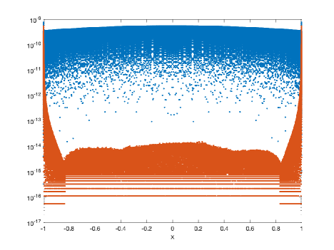
Experiment 1: Let us consider the function with to illustrate Thm. 5.2. According to this theorem, should be taken greater than . The numerical experiment shows that in this case the theorem is also valid when . We get that for , , the maximum error is divided by a factor approximately equal to when is increased by one. So the maximum error behaves as . This is true for and . Figure 1 illustrates this by plotting for and with . The curve for is above the one for .
So, one would think that increasing the value of is not a good idea. However, the factors between the errors for and are small and around . More importantly the error function for this function behaves much better for compared to . Figure 2 shows the error function for , and . The blue dots represent the error function for (original FH interpolants), the red dots for .
Although the peak increases slightly for increasing values of , the behaviour away from the origin is much better. We did not show the behaviour of the error function for . In this case the behaviour is between the behaviour for and .
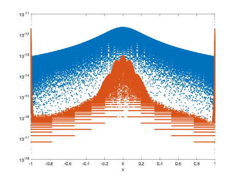
Experiment 2: Let us consider the function with . The conditions of Thm. 5.2 require that should be greater than to obtain a maximum error that behaves as . However, the numerical experiments indicate that this behaviour is also obtained for and . We have that for , , the maximum error is divided by a factor approximately equal to when is increased by one. So the maximum error behaves as . This is true for and . Figure 3 illustrates this by plotting for and with . The curve for is above the one for .
Also here, one would think that increasing the value of is not a good idea. However, the factors between the errors for and are also small and around . More importantly, the error functions in the case also behave much better for increasing values of . Figure 4 shows the error function for , and . The blue dots represent the error function for (original FH interpolants), the red dots for and so on.
Although the peak increases slightly for increasing values of , the behavior away from the origin is much better.
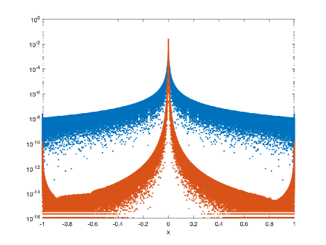
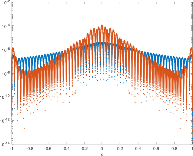
Experiment 3: Let us consider the analytic function . Figure 5 shows the error function for , and . The blue dots represent the error function for (original FH interpolants), the red dots for .
Following the theory, the maximum error for the interpolants should behave as when (cf. (3)). This can be also observed in practice for but for too, although Thm. 5.3 predicts a lower order of convergence when . The behavior in between the peaks is much better when compared to .
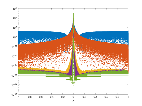
Experiment 4: Let us consider the analytic Runge-function . Figure 6 shows the error function for , and . The blue dots represent the error function for (original FH interpolants), the red dots for .
As in the previous experiment, according to (3), the maximum error for the interpolants behaves as when , and this is also observed for . Moreover, the behavior in between the peaks is much better when compared to . However, if we take a similar figure for we obtain Figure 7. In this case, performs worse compared to .
Experiment 5: In [10] an upper bound is derived for the Lebesgue constant in case :
| (105) |
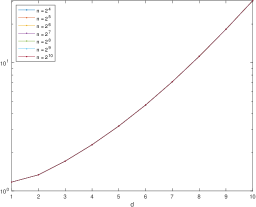
To illustrate this, in Figure 8 the Lebesgue constant is plotted in function of where the different lines correspond to values of (left) and in function of for different values of (right).
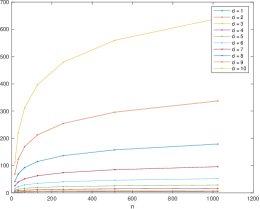
The left figure clearly demonstrates the factor in (105) while the right figure illustrates the dependency. Plotting similar figures for we obtain Figure 9.
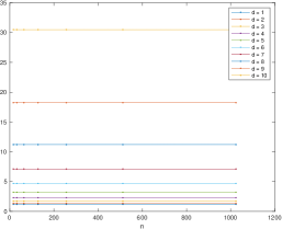
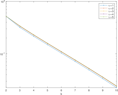
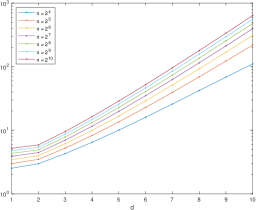
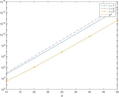
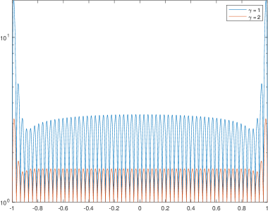
This figure shows that for the Lebesgue constant is independent of . For we obtain similar figures. In Figure 10 we plot the Lebesgue constant for , and for . We compare this behaviour with the plot . This figure shows that the Lebesgue constant behaves as with independent of .
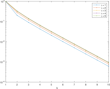
In Figure 11 the Lebesgue function is plotted for , and and .
Experiment 6: In this experiment, we compare the elapsed time of the classical Floater-Hormann algorithm with computing and evaluating the new approximant. We implemented the two algorithms in Matlab and measured the elapsed time using the tic - toc commands. We used the following values: , , and , the number of -values in which the approximant is evaluated. The weights for the classical barycentric form can be computed beforehand by FLOPS using (32) or in FLOPS using a more complicated pyramid algorithm [11]. We implemented the former method. Running the methods times and averaging, computing the weights for the classical FH approximant took seconds while evaluating it in the points costed seconds. Computing and evaluating the new approximant took seconds. For a different value of , we obtained comparable results.
7 Conclusion
In this paper, we have defined a whole family of generalized Floater–Hormann interpolants depending on an additional parameter , besides the usual parameter . For we obtain the original Floater–Hormann interpolants. The numerical examples show that this family has potential to approximate non-smooth as well as smooth functions. In future work, the (sub-)optimal choice of the parameters and could be investigated when the interpolation points are given. For the original Floater–Hormann interpolants Güttel and Klein [9] have developed a heuristic method to determine the parameter . To remedy the bad behaviour of the error function at the endpoints, Klein [13] designed a method adding some interpolation points at the two endpoints. A similar technique could be applied to the generalized Floater–Hormann approximants here introduced. However, this approach seems useful only when the interpolated function is periodic [6]. Moreover, in [7] it is shown that Klein’s method is numerically unstable. It could be interesting to investigate the well-conditioned case for all , looking for some improvement w.r.t. the cases studied in [1, 15]. This and the following questions are left for future research: (A) Refine the theoretical bound of the Lebesgue constant in (38) and also state a lower bound according to the numerical experiments; (B) Investigate the Lebesgue constants and the error for other configurations of nodes too; (C) Deeper explore the role of in view of the numerical experiments that suggest larger theoretical bounds on .
Acknowledgments
The authors wish to thank the anonymous reviewers for their valuable comments.
References
- [1] J.-P. Berrut. Rational functions for guaranteed and experimentally well-conditioned global interpolation. Computers & Mathematics with Applications, 15(1):1–16, 1988.
- [2] J.-P. Berrut and G. Klein. Recent advances in linear barycentric rational interpolation. Journal of Computational and Applied Mathematics, 259:95–107, 2014.
- [3] L. Bos, S. De Marchi, and K. Hormann. On the Lebesgue constant of Berrut’s rational interpolant at equidistant nodes. Journal of Computational and Applied Mathematics, 236(4):504–510, 2011.
- [4] L. Bos, S. De Marchi, K. Hormann, and G. Klein. On the Lebesgue constant of barycentric rational interpolation at equidistant nodes. Numerische Mathematik, 121:461–471, 2012.
- [5] A. P. Camargo. On the numerical stability of Floater–Hormann’s rational interpolant. Numerical Algorithms, 72:131–152, 2016.
- [6] A. P. Camargo. A comparison between extended Floater–Hormann interpolants and trigonometric interpolation. Dolomites Research Notes on Approximation, 10(DRNA Volume 10.1):23–32, 2017.
- [7] A. P. Camargo and W. F. Mascarenhas. The stability of extended Floater–Hormann interpolants. Numerische Mathematik, 136(1):287–313, 2017.
- [8] M. S. Floater and K. Hormann. Barycentric rational interpolation with no poles and high rates of approximation. Numerische Mathematik, 107:315–331, 2007.
- [9] S. Güttel and G. Klein. Convergence of linear barycentric rational interpolation for analytic functions. SIAM Journal on Numerical Analysis, 50(5):2560–2580, 2012.
- [10] K. Hormann, G. Klein, and S. De Marchi. Barycentric rational interpolation at quasi-equidistant nodes. Dolomites Research Notes on Approximation, 5:1–6, 2012.
- [11] K. Hormann and S. Schaefer. Pyramid algorithms for barycentric rational interpolation. Computer Aided Geometric Design, 42:1–6, 2016.
- [12] D. Huybrechs and L. N. Trefethen. AAA interpolation of equispaced data. BIT Numerical Mathematics, 63(2):21, 2023.
- [13] G. Klein. An extension of the Floater–Hormann family of barycentric rational interpolants. Mathematics of Computation, 82(284):2273–2292, 2013.
- [14] L. N. Trefethen. Approximation Theory and Approximation Practice. SIAM, 2012.
- [15] R.-J. Zhang and X. Liu. Rational interpolation operator with finite Lebesgue constant. Calcolo, 59(1):10, 2022.