Classical sampling from noisy Boson Sampling and the negative probabilities

Abstract

It is known that, by accounting for the multiboson interferences up to a finite order, the output distribution of noisy Boson Sampling, with distinguishability of bosons serving as noise, can be approximately sampled from in a time polynomial in the total number of bosons. The drawback of this approach is that the joint probabilities of completely distinguishable bosons, i.e., those that do not interfere at all, have to be computed also. In trying to restore the ability to sample from the distinguishable bosons with computation of only the single-boson probabilities, one faces the following issue: the quantum probability factors in a convex-sum expression, if truncated to a finite order of multiboson interference, have, on average, a finite amount of negativity in a random interferometer. The truncated distribution does become a proper one, while allowing for sampling from it in a polynomial time, only in a vanishing domain close to the completely distinguishable bosons. Nevertheless, the conclusion that the negativity issue is inherent to all efficient classical approximations to noisy Boson Sampling may be premature. I outline the direction for a whole new program, which seem to point to a solution. However its success depends on the asymptotic behavior of the symmetric group characters, which is not known.

I Introduction

Boson Sampling model AA is one of the proposals for near term quantum advantage with intermediate size quantum systems QSup , with the advantage that it does not involve interactions between quantum subsystems (individual bosons) with the promised quantum advantage over classical simulations coming solely from the Bose-Einstein statistics. On the experimental side, the photons are quite suitable source of non-interacting bosons and Boson Sampling with $N=20$ photons was recently demonstrated experimentally 20Ph60M , still short of the believed threshold $N\approx 50$ bosons QSBS ; Cliffords for the advantage over digital computers. Instead the focus shifted to the so-called Gaussian Boson Sampling GBS1 ; GBS2 with the squeezed states of light at input, which admits much better scalability in experiments ExpGBS2 . On the other hand, one has also to keep in mind the fact that realistic sources and other setup parts feature some amount of noise. Such are realistic photon sources, producing only partially indistinguishable photons, due to imperfect internal state matching or the optical path mismatch in propagation in a realistic interferometer. This and other sources of noise may severely affect the possible quantum advantage by allowing an approximate efficient classical sampling. In this respect the single-photon Boson Sampling model allows for an analytical analysis of how the quantum advantage is affected by the inevitable experimental noise due to uncontrolled partial distinguishability of photons. There is the classical limit, the completely distinguishable photons. In Ref. R1 it was shown that by employing a cut-off on the higher-orders of multi-photon interferences and simulating classically the resulting approximate model one can efficiently sample classically, to a small $N$-independent error, from such a noisy Boson Sampling. Similar approach can be employed for other noise sources, such as noise in interferometer LP ; KK ; Arkh due to the equivalence links between different noise models VS2019 . The approach of Ref. R1 requires efficient computation of the joint transition probabilities of completely distinguishable bosons by employing the JSV algorithm JSV . However, this is a strange feature of a sampling algorithm, since completely distinguishable bosons behave as classical particles: they can be sampled from in linear time, e.g., by sending particles one by one through the interferometer.

To investigate whether one can do better that the algorithm of Ref. R1 , especially in dealing with the classical particles, is the main objective of the present work. One would expect, as a better algorithm, an algorithm which is polynomial in the total number of bosons for any finite value of the distinguishability parameter and which does not rely on computing the probabilities of joint transitions of the completely distinguishable bosons (classical particles). An algorithm which satisfies the second condition was presented in Ref. Moy , however, it cannot be a polynomial algorithm in the total number of bosons for a finite distinguishability parameter.

The text is organized as follows. In the next section, section II, I summarize the appropriate description of partially distinguishable bosons VS2014 ; PartDist , and formulate the condition for the partial distinguishability function for the proper probability distribution. In section III I recall the approach of Ref. R1 of simulating Boson Sampling with multi-boson interferences up to a fixed order $R$ and the reasons why it works. In section IV, the quantum probability factor truncated to lower-order interference terms is shown to have some finite negativity, thus preventing direct sampling from the convex-sum expansion for probability. In section V, it is shown that the approach of Ref. R1 produces a proper probability distribution if the distinguishability parameter satisfies $x\leq\frac{1}{N-K}$ for a free parameter $K$, at a heavy price of the sampling complexity scaling as $O(K^{2}4^{K})$. Finally, in section VI I outline the direction for a new program, which might permit one to find proper approximating distributions for the noisy Boson Sampling distribution. Section VI contains a short summary of the results.

II Models of distinguishability with proper probability distributions

Boson Sampling model performs unitary transformation $U$ of size $M\times M$ on the Fock state of $N$ indistinguishable bosons in different input ports, say $k=1,\ldots,N$ to an output Fock state in the so-called no-collision regime, when all bosons end up in different output ports $l_{1},\ldots,l_{N}$ (the odds to have this in a random multiport is estimated to be $1-O(N^{2}/M)$ AA ). The output probability is given by the product of the quantum amplitude of the transition and its complex conjugate,

$$p(l_{1},\ldots,l_{N})=\left|\sum_{\sigma}\prod_{k=1}^{N}U_{\sigma(k),l_{k}}\right|^{2}$$ (1)

$$=|\mathrm{per}U[1,\ldots,N|l_{1},\ldots,l_{N}]|^{2},$$

where the amplitude is given by the matrix permanent Minc , i.e., the summation is over all permutations $\sigma$ of $N$ objects (a.k.a. the symmetric group $S_{N}$).

Realistic description of a physical setup (e.g., with photons) must account for distinguishability of bosons. This can be done by introducing a single function $J(\sigma)$ on the symmetric group $S_{N}$, called the distinguishability function, which weights the path-dependent interferences of $N$ bosons in a quantum amplitude and its conjugate for different permutations $\sigma$, i.e., the expression in Eq. (1) generalizes VS2014 ; PartDist as follows

$$p^{(J)}(l_{1},\ldots,l_{N})=\sum_{\sigma_{1},\sigma_{2}}J(\sigma_{1}\sigma_{2}^{-1})\prod_{k=1}^{N}U^{*}_{\sigma_{1}(k),l_{k}}U_{\sigma_{2}(k),l_{k}}.$$ (2)

The distinguishability function $J(\sigma)$ reflects the internal states of bosons, described by the density matrix $\hat{\rho}^{(N)}\in H^{\otimes N}$, in the tensor product of Hilbert spaces $H$ of each boson, and is given by the trace-product with the unitary representation $\hat{P}_{\sigma}$ of $\sigma$ in $H^{\otimes N}$:

$$J(\sigma)=\mathrm{tr}\left(\hat{P}_{\sigma}\hat{\rho}^{(N)}\right).$$ (3)

When the internal state is completely symmetric, i.e. $\hat{P}_{\sigma}\hat{\rho}^{(N)}=\hat{\rho}^{(N)}$, the bosons in the $\hat{\rho}$ are completely indistinguishable VS2014 ; PartDist , and we get the probability as in Eq. (1); the completely distinguishable bosons correspond to $J(\sigma)=\delta_{\sigma,I}$, where $I$ is the trivial permutation, with the probability in Eq. (2) being equal to the matrix permanent of a positive matrix with elements $|U_{kl}|^{2}$.

The $J$-function of Eq. (3) is positive definite, i.e., for an arbitrary function $Z_{\sigma}$ on $S_{N}$ we have

$$\sum_{\sigma_{1},\sigma_{2}}J(\sigma_{1}\sigma_{2}^{-1})Z_{\sigma_{1}}Z^{*}_{\sigma_{2}}\geq 0.$$ (4)

Observe that Eq. (4) presupposes that $J^{*}(\sigma)=J(\sigma^{-1})$ readily satisfied by $J(\sigma)$ of Eq. (3) due to the unitarity of the symmetric group representation, $P^{\dagger}_{\sigma}=P_{\sigma^{-1}}$. The group property $\hat{P}_{\sigma_{1}\sigma^{-1}_{2}}=\hat{P}_{\sigma^{-1}_{1}}\hat{P}{\sigma_{2}}$ guarantees the positive definiteness of $J$ in Eq. (3):

$$\mathrm{tr}\left(\sum_{\sigma_{1}}Z_{\sigma_{1}}\hat{P}_{\sigma_{1}}\hat{\rho}^{(N)}\sum_{\sigma_{2}}Z^{*}_{\sigma_{2}}\hat{P}^{\dagger}_{\sigma_{2}}\right)\geq 0,$$ (5)

since the density matrix of the internal state of bosons $\hat{\rho}$ is a positive definite operator in $H^{\otimes N}$. Another important property is the normalization $J(I)=1$ (i.e., the sum of probabilities must be equal to $1$). These two properties guarantee that the probabilities in Eq. (2) constitute a proper distribution. It has been shown in Ref. PRL2016 that all normalized positive definite functions on the symmetric group $S_{N}$ can be represented in the form of Eq. (3) with some (possibly entangled) mixed state $\hat{\rho}\in H^{\otimes N}$ of $N$ single bosons. Thus one can on choice work either with the internal state $\hat{\rho}$ or with the distinguishability function description in dealing with partially distinguishable bosons.

On the other hand performing an arbitrary approximation in the expression for the proper probability distribution may result in a non-proper one. The model of Ref. R1 is obtained by considering that bosons are in some pure internal states having a uniform cross-state overlap $x$, or, alternatively, considering that the boson at input port $k$ is in the following mixed state

$$\hat{\rho}_{k}=x|\phi_{0}\rangle\langle\phi_{0}|+(1-x)|\phi_{k}\rangle\langle\phi_{k}|,\quad\langle\phi_{i}|\phi_{j}\rangle=\delta_{ij},$$ (6)

in this case $\hat{\rho}^{(N)}=\hat{\rho}_{1}\otimes\ldots\otimes\hat{\rho}_{N}$ (see also Ref. VS2019 ). A non-proper approximation to the proper distribution is obtained in Ref. R1 by imposing a cut-off on the two sums in Eq. (2), such that the minimum number of fixed points in the relative permutation (i.e., the number of $1$-cycles $C_{1}$) is bounded from below: $C_{1}(\sigma_{1}\sigma^{-1}_{2})\geq N-R$ for some fixed ($N$-independent) $R$. The distinguishability function $J_{N}(\sigma)=x^{N-C_{1}(\sigma)}$ of the model in Eq. (6) is replaced accordingly by the following function

$$J_{R}(\sigma)=\sum_{m=N-R}^{N}x^{N-m}\delta_{C_{1}(\sigma),m},$$ (7)

which does not satisfy the positivity property of Eq. (4). To see this and the underlying reason for lost positivity, let us formulate more general condition of positivity valid for all models of similar type, i.e.,

$$F(\sigma)=\sum_{m=0}^{N}a_{m}\delta_{C_{1}(\sigma),m},$$ (8)

where $a_{m}$ are real parameters satisfying the normalization condition $F(I)=1$, i.e., $a_{N}=1$. To this goal we expand $\delta_{C_{1}(\sigma),m}$ over the partitions of the set $1,\ldots,N$ into the variable set of $m$ fixed points $\mathbf{k}^{(m)}=(k_{1},\ldots k_{m})$ and its complement (i.e., the set of derangements). Then

$$\delta_{C_{1}(\sigma),m}=\sum_{\mathbf{k}^{(m)}}\left(\prod_{k\in\mathbf{k}^{(m)}}\delta_{\sigma(k),k}\right)\prod_{k\notin\mathbf{k}^{(m)}}(1-\delta_{\sigma(k),k})$$

$$=\sum_{n=m}^{N}\binom{n}{m}(-1)^{n-m}\sum_{\mathbf{k}^{(n)}}\prod_{k\in\mathbf{k}^{(n)}}\delta_{\sigma(k),k},$$ (9)

where we have expanded the second factor and combined the fixed points into a bigger set $\mathbf{k}^{(n)}$ of size $n$. Now we substitute the expansion of Eq. (II) into the model Eq. (8) and exchange the order of summation

$$F(\sigma)=\sum_{m=0}^{N}a_{m}\delta_{C_{1}(\sigma),m}$$

$$=\sum_{n=0}^{N}\sum_{m=n}^{N}\binom{n}{m}(-1)^{n-m}a_{m}\prod_{k\in\mathbf{k}^{(n)}}\delta_{\sigma(k),k}.$$ (10)

For the function in Eq. (II) to be positive definite it is sufficient to require the coefficients at the functions $j_{\mathbf{k}^{(n)}}(\sigma)=\prod_{k\in\mathbf{k}^{(n)}}\delta_{\sigma(k),k}$ to be positive, since $j_{\mathbf{k}^{(n)}}(\sigma)$ is a positive definite function, e.g., for $\mathbf{k}^{(n)}=(1,\ldots,n)\equiv[n]$ we have the following representation

$$j_{[n]}(\sigma)=\mathrm{Tr}\left\{\hat{P}_{\sigma}\prod_{k=1}^{n}{}^{\otimes}|\phi_{k}\rangle\langle\phi_{k}|\otimes\left(|\phi_{0}\rangle\langle\phi_{0}|\right)^{\otimes N-n}\right\},$$ (11)

with $\langle\phi_{i}|\phi_{j}\rangle=\delta_{ij}$, which is obviously positive definite. Setting the coefficients at the positive definite functions $j_{\mathbf{k}^{(n)}}(\sigma)$ in Eq. (II) to be

$$b_{n}\equiv\sum_{m=0}^{n}\binom{n}{m}(-1)^{n-m}a_{m}$$ (12)

and inverting the summation in their definition we get the conditions for the positivity of the function $F(\sigma)$ in Eq. (II):

$$a_{m}=\sum_{n=0}^{m}\binom{m}{n}b_{n},\quad b_{n}\geq 0.$$ (13)

Therefore, among the functions $F(\sigma)$ in the form given by Eq. (II) the functions

$$F^{(+)}(\sigma)=\sum_{n=0}^{N}b_{n}\sum_{m=n}^{N}\binom{m}{n}\delta_{C_{1}(\sigma),m},\quad b_{n}\geq 0$$ (14)

are positive definite functions on $S_{N}$.

The partial distinguishability model of Ref. R1 , i.e., $J_{N}(\sigma)=x^{N-C_{1}(\sigma)}$, can be also cast in the form of Eq. (14) with $b_{n}=x^{N-n}(1-x)^{n}$ (observe that $0\leq x\leq 1$, see Eq. (6)), which fact can be directly verified by exchanging the summation and using the binomial theorem.

The physical interpretation of the condition in Eq. (14) follows from application of the expansion of Eq. (II) for each term with positive coefficient in Eq. (14). We obtain the relation

$$\sum_{m=n}^{N}\binom{m}{n}\delta_{C_{1}(\sigma),m}=\sum_{\mathbf{k}^{(n)}}\prod_{k\in\mathbf{k}^{(n)}}\delta_{\sigma(k),k}=\sum_{\mathbf{k}^{(n)}}j_{\mathbf{k}^{(n)}}(\sigma).$$ (15)

When substituted into the output probability distribution of Eq. (2), the basic distinguishability function $j_{\mathbf{k}^{(n)}}(\sigma)$ imposes the same permutation of bosons in the quantum amplitude and its conjugate, $\sigma_{1}(k)=\sigma_{2}(k)$ for $k\in\mathbf{k}^{(n)}$, i.e., the bosons from the inputs $k\in\mathbf{k}^{(n)}$ behave as completely distinguishable bosons (i.e., as classical particles), and the output probability factorizes into a product of those for $N-n$ indistinguishable and $n$ distinguishable bosons. Similarly, in the case of $J$-function of Ref. R1 , i.e., $J_{N}(\sigma)=x^{N-C_{1}(\sigma)}$ the probability of Eq. (2) expands as follows (exchanging $n$ and $N-n$, for future convenience)

$$p^{(J_{N})}(l_{1}\ldots l_{N})=\sum_{n=0}^{N}x^{n}(1-x)^{N-n}$$

$$\times\sum_{\mathbf{l}^{(n)}}\sum_{\mathbf{k}^{(n)}}p^{(J_{N},x=1)}(\mathbf{l}^{(n)}|\mathbf{k}^{(n)})\mathrm{per}|U|^{2}[\mathbf{l}^{(N-n)}|\mathbf{k}^{(N-n)}],$$

where $(\mathbf{k}^{(n)},\mathbf{k}^{(N-n)})$ and $(\mathbf{l}^{(n)},\mathbf{l}^{(N-n)})$ are some permutations of $[N]$, the subset $\mathbf{l}^{(n)}=(l_{\alpha_{1}},\ldots,l_{\alpha_{n}})$ is the set of output ports of $n$ indistinguishable bosons ($J_{N}=1$ for $x=1$), and $\mathrm{per}|U|^{2}[\mathbf{l}^{(N-n)}|\mathbf{k}^{(N-n)}]$ is the classical probability (the matrix permanent of the matrix $|U_{kl}|^{2}$), which can be cast in the form of Eq. (2) with $J_{0}(\sigma)=\delta_{\sigma,I}$ (see Ref. VS2019 for more details).

The cut-off model with $J_{R}$ of Eq. (7) does not satisfy the positive definiteness condition formulated in Eq. (14), which fact can imply that the approximation with such a distinguishability function does allow some probabilities to be negative (note that the normalization condition $J_{R}(I)=1$ is satisfied, thus the probabilities must sum to $1$). From Eqs. (7) and (15), by comparing with Eq. (II), one can expand the probability of the cut-off model as follows

$$p^{(J_{R})}(l_{1}\ldots l_{N})=\sum_{n=0}^{N}x^{n}(1-x)^{N-n}$$

$$\times\sum_{\mathbf{l}^{(n)}}\sum_{\mathbf{k}^{(n)}}p^{(J_{R},x=1)}(\mathbf{l}^{(n)}|\mathbf{k}^{(n)})\mathrm{per}|U|^{2}[\mathbf{l}^{(N-n)}|\mathbf{k}^{(N-n)}],$$

where $p^{(J_{R},x=1)}(\mathbf{l}^{(n)}|\mathbf{k}^{(n)})$ is given by Eq. (2) with the $J_{R}$ of Eq. (7) for $x=1$ and may become negative. Since, by the expression in Eq. (2), it involves some mutually dependent diagonals of $U$ (here the “diagonal” is a product of elements of $U$ on distinct rows and distinct columns), such as $Z_{\sigma}=\prod_{k=1}^{n}U_{\sigma(k),l_{k}}$ (with $\sigma\in S_{n}$), having only up to $n^{2}$ free parameters instead of $n!$ in an arbitrary $Z_{\sigma}$, we need to find out the amount of negativity in the subspace spanned by above diagonals, and not in the entire $n!$-dimensional vector space of $Z_{\sigma}$.

As $N\to\infty$, for a finite $x=O(1)$ one can estimate the number of computations for the direct sampling from the output distribution in the form of Eq. (II) by observing that the binomial distribution $\binom{N}{n}x^{n}(1-x)^{N-n}$ becomes sharply concentrated in the small interval of size $O(\sqrt{x(1-x)N})$ centered at $\overline{n}=xN$. Thus computations of the matrix permanents of the average size $xN$ are required for sampling at an error vanishing as $O(N^{-\frac{1}{2}})$. Therefore, by similar arguments as in Ref. Cliffords , asymptotically in $N$, the sampling complexity can be estimated to be the same as that of the ideal Boson Sampling with only $xN$ bosons (similar observation was used in Ref. Moy ). This observation sets the base lime for the number of computations in an approximate model, such as Eq. (II).

III Approximate classical simulation of partially distinguishable bosons

Let us now recall the main ideas of Ref. R1 for the efficient approximate classical simulation of Boson Sampling with partially distinguishable bosons. In the exposition of some of the essential steps we will follow also Ref. VS2019 . They are as follows.

(I).– One considers the total variation distance $\mathcal{D}=\frac{1}{2}\sum|p^{(J_{N})}-p^{(J_{R})}|$ between the distributions in Eqs. (II) and (II) averaged over the random multiports $U$ chosen according to the Haar measure. For $M\gg N^{2}$, up to a small error, one can use the Gaussian approximation with independent Gaussian distribution for each $U_{kl}$ AA instead. In the latter case it can be shown that (see derivation in Ref. VS2019 )

$$\langle\mathcal{D}\rangle_{U}<\frac{1}{2}\sqrt{1+\frac{e}{(R+2)!}}\frac{x^{R+1}}{\sqrt{1-x^{2}}}.$$ (18)

Having shown that the two probability distributions, one proper and one improper, are close on average, one can then use the Markov inequality in the probability to bound the total variation distance at the cost of some non-zero probability of failure R1 .

(II).– One show that the total amount of computations necessary for obtaining a single probability for the cut-off model scale as $O(R2^{R}N^{2R})$ and the small fixed error requires only $R=O(1)$. For this goal one can use the expression in Eq. (2) substituting the distinguishability function of Eq. (7) expressed as a sum over the derangements $J_{R}(\sigma)=\sum_{n=0}^{R}x^{n}\mathcal{I}(D^{(N)}_{n})$, where $\mathcal{I}(D^{(N)}_{n})$ is the indicator on the subset $D^{(N)}_{n}$ of permutations in $S_{N}$ with $N-n$ fixed points, i.e., the derangements of $n$ elements. The described expansion reads (we suppress the output port indices; see also Ref. R1 )

$$p^{(J_{R})}=\sum_{n=0}^{R}x^{n}\mathcal{U}(D^{(N)}_{n}),$$

$$\mathcal{U}(D^{(N)}_{n})\equiv\sum_{\sigma\in D^{(N)}_{n}}\sum_{\tau}\prod_{k=1}^{N}U^{*}_{\sigma[\tau(k)],l_{k}}U_{\tau(k),l_{k}}.$$ (19)

By splitting the input $N$ indices into the $n$ derangements, $\mathbf{k}^{(n)}$, and $N-n$ fixed points, $\mathbf{k}^{(N-n)}$, we can expand the expression in Eq. (III) as follows

$$\mathcal{U}(D^{(N)}_{n})=\sum_{\mathbf{k}^{(n)}}\sum_{\mathbf{l}^{(n)}}\mathcal{U}(D^{(n)}_{n})\mathrm{per}|U|^{2}(\mathbf{k}^{(N-n)}|\mathbf{l}^{(N-n)}),$$ (20)

where the summation over the partition $(\mathbf{l}^{(n)},\mathbf{l}^{(N-n)})$ of the output ports appears as the result of factoring the second permutation in the probability formula in Eq. (III) $\tau=(\tau_{1}\otimes\tau_{2})\mu$ with $\mu\in\frac{S_{N}}{S_{n}\otimes S_{N-n}}$ and $\tau_{1}\in S_{n}$ and $\tau_{2}\in S_{N-n}$, acting on $\mathbf{l}^{(n)}$ and $\mathbf{l}^{(N-n)}$, respectively. Now, the first factor $\mathcal{U}(D^{(n)}_{n})$ in Eq. (20) contains only the derangements $D^{(n)}_{n}\subset S_{n}$, in the subset of indices $\mathbf{k}^{(n)}$, and the second factor only the fixed points (a probability of $N-n$ classical particles). The derangements do not represent any probability at all (they appear in complex conjugate pairs, since the inverse permutation to a derangements in $D_{n}$ is also a derangements in the same subset $D_{n}$). They can be computed using either Ryser or Glynn algorithm (see also section IV below, where such computations are discussed in detail for another purpose – checking the negativity), whereas the classical probabilities are estimated to a small relative error $\epsilon$ by the probabilistic JSV algorithm JSV in the polynomial time in $(N-n,1/\epsilon)$.

(III).– One can sample from the approximate probability distribution Eq. (II) by using the algorithm similar to that of. Ref. Cliffords if one can compute the probability with an acceptable relative error, i.e., on the order of the bound on the total variation distance. However, though the cut-off model does not satisfy the positivity constraint of Eq. (14), the negativity is automatically bounded as desired. Indeed, when two distributions, one proper and one improper, are at some total variation distance $\epsilon$, the amount of negativity (some of the negative probabilities) is bounded by $2\epsilon$, by the simple fact that the total if variation distance is the maximum of the difference in probability. It still remains to find out the effect of the relative error introduced by the probabilistic JSV algorithm. In Ref. R1 the average difference in probability $\langle|p^{(J=1)}-p^{(J_{R})}|\rangle$ for a given output is bounded. Since the average probability $\langle p^{(J=1)}\rangle=\langle p^{(J)}\rangle$ in a random $U$ is uniform, the maximum relative error in a probability, including that introduced by the JSV algorithm, becomes the absolute error on the total variation distance. Thus the maximum relative error in probability becomes the absolute error on the total variation distance (similar as for the ideal case of Boson Sampling AA ; this feature for partially distinguishable bosons has been discussed before in Ref. VS2014 ).

For the discussion below, let us recall the key points on the averaging of the individual terms in the sum over the derangements, $\mathcal{U}(D^{(N)}_{n})$, in Eq. (III)

$$T(\sigma)\equiv\sum_{\tau}\prod_{k=1}^{N}U^{*}_{\sigma[\tau(k)],l_{k}}U_{\tau(k),l_{k}},$$ (21)

over the Haar-random multiport (in the Gaussian approximation for $M\gg N^{2}$; below we follow the derivation in Ref. VS2019 ). We have

$$\langle T(\sigma)\rangle_{U}=\delta_{\sigma,I}\frac{N!}{M^{N}},$$

$$\langle T(\sigma)T^{*}(\pi)\rangle_{U}=\delta_{\sigma,\pi}\frac{N!}{M^{2N}}\chi(C_{1}(\sigma)),$$ (22)

where $\chi(n)=n!\sum_{k=0}^{n}\frac{1}{k!}$. The first line in Eq. (III) gives the non-zero average of a product of independent Gaussian random variables from a diagonal of $U$ and that of $U^{*}$ coinciding only for $\sigma=I$. The second line in Eq. (III) follows from a result in Appendix A of Ref. VS2014 on the averaging of a product of four diagonals, two of $U$ and two of $U^{*}$:

$$\langle\prod_{k=1}^{N}U^{*}_{\sigma[\tau(k)],l_{k}}U_{\tau(k),l_{k}}U^{*}_{\sigma^{\prime}[\tau^{\prime}(k)],l_{k}}U_{\tau^{\prime}(k),l_{k}}\rangle_{U}$$

$$=\frac{2^{C_{1}(\pi)}}{M^{2N}}\delta_{\sigma^{\prime},\sigma^{-1}}\delta_{\tau^{\prime},(\pi\otimes I)\sigma\tau},$$ (23)

where in the second delta-symbol permutation $\pi$ acts on the fixed points and $I$ on the derangements of $\sigma$. The factor $N!$ in Eq. (III) accounts for the sum over $\tau\in S_{N}$ in Eq. (III), whereas $\chi(n)$ is the sum over $\pi\in S_{C_{1}(\sigma)}$ as follows

$$\chi(n)=\sum_{\pi\in S_{n}}2^{C_{1}(\pi)}=\int\limits_{1}^{\infty}\mathrm{d}te^{1-t}t^{n}.$$ (24)

We have uncorrelated terms $T(\sigma)$ in the summation in Eq. (III), where only the classical term $T(I)$ has a non-zero average. The same applies to similar terms in $\mathcal{U}(D^{(n)}_{n})$ in Eq. (20) (with $N$ substituted by $n$), with the average being always zero. The bound in Eq. (18) follows from the bound on the probability difference $X=|p^{(J_{N})}-p^{(J_{R})}|$ by its variance $\langle X\rangle\leq\sqrt{\langle X^{2}}\rangle$, where the second moment is the variance due to the same average probability. Moreover, the square root of the variance is bounded by the inverse total number $\frac{N!}{M^{N}}$ of the probabilities in the output probability distribution (in the no-collision regime). These observations allow for derivation of the bound in Eq. (18).

The approach of Ref. R1 leads to an approximate sampling algorithm for partially distinguishable bosons, at least in the model considered in Eq. (7). Our main goal below is investigate whether one can do any better. For instance, can one find any other expansion of the same probability, alternative to that of Eq. (III) in order to implement sampling from the classical probabilities in linear time, instead of employing numerically intricate probabilistic JSV algorithm? Such an alternative expansion will be discussed in the following section.

The model of Eq. (6) is also applicable to the experimental Boson Sampling with photons (the most important reason to keep the model for further discussion). It can serve as description of the realistic optical setup, since one has infinite number of free parameters in a photon state (its spectral shape), and the experimental photons are described by mixed states. If we assume that the latter are close with probability $x$ to a pure state $|\phi_{0}\rangle$ and have a long tail over the orthogonal complement, then in Eq. (6) the orthogonal complementary states $|\phi_{i}\rangle$, one for each photon, describe $N$ states selected at random from the infinite-dimensional subspace of the states orthogonal to $|\phi_{0}\rangle$.

IV Estimating the negativity

Below a numerical evidence of negativity in the quantum factors in the convex sum expansion of the output probability distribution is presented. There are two types on negativity: the negativity in the approximate probability distribution, reported in Ref. R1 , and the negativity in a factor in the convex-sum expression in Eq. (II). The latter negativity will be numerically estimated below, it prevents direct sampling from the convex-sum expression of the approximate probability and forces one to resort to the JSV algorithm for computation of the classical probabilities.

The probability factor $p^{(J_{R},x=1)}(\mathbf{l}^{(n)}|\mathbf{k}^{(n)})$ in Eq. (II) has $J_{R}$ of Eq. (7) now for a variable number of bosons $n$ satisfying $n\geq R$ (for $n<R$ the quantum probability is positive) and $x=1$. As discussed in section II, the lack of the positive definiteness of the distinguishability function causes some of $p^{(J_{R},x=1)}(\mathbf{l}^{(n)}|\mathbf{k}^{(n)})$ to become negative. But how much negativity is there? Since this depends on the multiport matrix $U$ projection on the negative subspace of the non-positive definite distinguishability function $J_{R}(\sigma_{1}\sigma^{-1}_{2})$, considered as the matrix element indexed by permutations $\sigma_{1},\sigma_{2}$ as in Eqs. (2) and (4), one can resort to numerical simulations to estimate negativity on average in a randomly chosen multiport $U$. We only have to calculate the probability for $\mathbf{l}^{(n)}=\mathbf{k}^{(n)}=(1,\ldots,n)$ (since we consider a randomly chosen multiport $U$)

$$p^{(J_{R},x=1)}=\sum_{s=0}^{R}\mathcal{U}(D^{(n)}_{s}),$$

$$\mathcal{U}(D^{(n)}_{s})=\sum_{\sigma\in D^{(n)}_{s}}\sum_{\tau\in S_{n}}\prod_{k=1}^{n}U^{*}_{\sigma[\tau(k)],k}U_{\tau(k),k}.$$ (25)

Before proceeding to discuss the numerical data, let us see what one can expect by trying an analytical analysis. To this goal we can apply the averaging over Haar-random multiport $U$ by employing the Gaussian approximation given by Eqs. (21)-(III) in order to estimate the variance. First of all, let us apply this approach to the full quantum probability $p^{(J=1)}$ (using $n$ temporarily as the total number of bosons), obtained by setting $R=n$ in Eq. (IV), i.e., to a positive probability. We get the following results (derived before in Ref. AA ):

$$\langle p^{(J=1)}\rangle_{U}=\langle\sum_{s=0}^{n}\mathcal{U}(D^{(n)}_{s})\rangle_{U}=\sum_{s=0}^{n}\delta_{s,0}\frac{n!}{M^{n}}=\frac{n!}{M^{n}}$$ (26)

and

$$\langle{p^{(J=1)}}^{2}\rangle_{U}=\langle\sum_{s,t=0}^{n}\mathcal{U}(D^{(n)}_{s})\mathcal{U}(D^{(n)}_{t})\rangle_{U}$$

$$=\frac{n!}{M^{2n}}\!\sum_{\sigma}\chi(C_{1}(\sigma))=\frac{n!}{M^{2n}}\int\limits_{1}^{\infty}\mathrm{d}te^{1-t}\sum_{\sigma}t^{C_{1}(\sigma)}$$

$$=(n+1)\left(\frac{n!}{M^{n}}\right)^{2},$$ (27)

where the cycle sum over the symmetric group has been used Stanley

$$\sum_{\sigma\in S_{n}}t^{C_{1}(\sigma)}=\left(\frac{\mathrm{d}}{\mathrm{d}z}\right)^{n}_{z=0}\frac{e^{(t-1)z}}{1-z}$$

to perform the integration over $t$. Moreover, the terms with different derangements $\mathcal{U}(D^{(n)}_{0}),\ldots,\mathcal{U}(D^{(n)}_{n})$ are mutually uncorrelated by Eq (V) (since the subsets of the respective permutations are non-overlapping), each contributing to the variance the square of the average of the classical term (with $\sigma=I$) $\langle\mathcal{U}(D^{(n)}_{0})\rangle=\frac{n!}{M^{n}}$. The above calculation illustrates the following point: in the Gaussian approximation of the Haar-random multiport $U$, the positive by definition probability is a sum of $n+1$ uncorrelated random variables with only the classical term having non-zero average (equal to the average probability) and the rest with zero average. The probability of the partially distinguishable bosons with $J_{R}$ of Eq. (7) is also composed of the same random variables, with, however, one important difference: they are multiplied by the respective powers of $x<1$, thus the variances are weighted accordingly. This observation allows to estimate the average total amount of negativity in the cut-off model, reported before in Ref. R1 : it is bounded by the square root of the variance of the terms subtracted from the full quantum probability, i.e. the terms with $s=R+1\ldots,n$, multiplied by the respective powers of $x$, i.e., the same bound as in Eq. (18).

Now we can return to the probability factor given in Eq. (IV). In this case $x=1$, therefore, the terms subject to the cut-off are not weighted by the powers of a small parameter. In this case it is tempting to conclude that there is a finite amount of negativity. On the other hand, if we apply the same arguments to the full quantum probability, we would get the same conclusion. The error of such conclusion lies in the assumption that uncorrelated terms contribute independently, but random variables can be uncorrelated and still dependent one on the other (e.g., in a nonlinear way: take $x$ and $x^{2}$ for a random $x$ with the symmetry $x\to-x$). Therefore, though the above arguments allow one to explain a small amount of negativity in the cut-off model due the higher powers of a small parameter $x$, they do not allow us to conclude on the negativity in the probability in Eq. (IV). One must therefore resort to numerical simulations.

To numerically compute the sums involving averaging over the derangements $\sigma$ in Eq. (IV) we adopt the method employed for computation of the matrix permanents Ryser ; Glynn (i.e., for averaging over the whole symmetric group). One way is to use the inclusion-exclusion principle when averaging over the symmetric group as in Ryser’s algorithm Ryser . Denoting by $\mathbf{l}^{(t)}$ the excluded subset of size $t$ from $[n]=\{1,\ldots,n\}$, we have

$$\sum_{\tau\in S_{n}}\prod_{k=1}^{n}U^{*}_{\sigma[\tau(k)],k}U_{\tau(k),k}$$

$$=\sum_{t=0}^{n-1}(-1)^{t}\sum_{\mathbf{l}^{(t)}}\prod_{k=1}^{n}\left(\sum_{l\notin\mathbf{l}^{(t)}}U^{*}_{\sigma(k),l}U_{kl}\right)$$ (28)

(for $t=n$ the product of diagonals becomes empty). Now we need to perform the second summation over the derangements $\sigma\in D^{(n)}_{s}$ in Eq. (IV). To this goal we introduce a tensor function $W(\xi)$ of a dummy variable $\xi$ as follows:

$$U^{*}_{j,l}U_{kl}\rightarrow W_{j,k,l}(\xi)=\left\{\begin{array}[]{cc}U^{*}_{j,l}U_{kl},&j\neq k;\\ \xi|U_{kl}|^{2},&j=k.\end{array}\right.$$ (29)

With this definition, the average over the derangements in Eq. (IV) becomes a Taylor expansion term in $\xi$ of the respective average over the symmetric group,

$$\sum_{\sigma\in D^{(n)}_{s}}\prod_{k=1}^{n}U^{*}_{\sigma(k),k}U_{k,k}$$

$$=\frac{1}{s!}\left(\frac{d}{d\xi}\right)^{s}_{\xi=0}\sum_{\sigma\in S_{n}}\prod_{k=1}^{n}W_{\sigma(k),k,l}(\xi),$$ (30)

to which we can apply the same inclusion-exclusion method as in Eq. (IV). Finally, combining the two independent summations in Eqs. (IV) and (IV) and evaluating the derivative of the polynomial function in $\xi$ by an appropriate averaging over the discrete phase $\xi=e^{i\theta(q)}$, where $\theta(q)=\frac{2\pi}{n+1}q$ and $q=0,\ldots,n$, we obtain the final formula for the double sum as follows

$$\mathcal{U}(D^{(n)}_{s})=\frac{1}{n+1}\sum_{q=0}^{n}e^{-i\theta(q)s}\sum_{t=0}^{n-1}(-1)^{t}\sum_{\mathbf{l}^{(t)}}\sum_{f=0}^{n-1}(-1)^{f}\sum_{\mathbf{k}^{(f)}}$$

$$\prod_{k=1}^{n}\left(\sum_{l\notin\mathbf{l}^{(t)}}\sum_{j\notin\mathbf{k}^{(f)}}W_{j,k,l}(e^{i\theta(q)})\right).$$ (31)

To reduce the number of computations one can perform summation in Eq. (IV) of the exponent over $s$ from the required set before summations over the inclusion-exclusion sets. The same approach can be used to adopt Glynn’s algorithm Glynn with some advantage of using the recursive computations as in Ref. Cliffords . The above algorithm requires $O(n^{2}4^{n})$ computations, where the base $4$ is due to the double summation over the inclusion-exclusion sets. It allows to compute the probability distribution over the Haar-random multiport on a personal computer for small number of bosons ($n\leq 12$).

The results of numerical simulations are presented in Fig. 1, where we give the distribution of the probability factor in Eq. (IV) over the complex-valued matrices with independent Gaussian-distributed elements (in total $5000$ matrices were used) for $n=7$ and $R=4$. Similar distributions in a random multiport was observed for other values of $n$ and various $R<n$. The odds of having a negative probability in a random multiport remain bounded by $\sim 10\%$ for all sets of $n$ and $R$ used in the simulations. Since the numerical simulations are limited to small $n$, thus one cannot make any definite conclusions on the negativity behavior for large numbers $n\sim N\gg 1$.

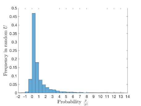
Figure 1: Histogram of the probability in Eq. (IV) in a random interferometer $U$. Here $n=7$ and $R=4$ the histogram is obtained by boxing of the probabilities by their relative occurrence in a randomly chosen multiport from the $5000$ of randomly generated unitary multiports according to the Haar measure.

V Positivity of the cut-off model

In section III we have two equivalent representations of the cut-off model of distinguishability, with the function $J_{R}$ of Eq. (7), one is given in Eqs. (II) and the other in Eqs. (III)-(20). Let us find out whether it admits yet another form, where the derangements are incorporated into some full probabilities that, at least in the majority of cases (recall that the whole distribution is improper, it allows for negative content on the order of the cut-off error), can be positive and this fact would allow one to avoid usage of the probabilistic JSV algorithm for the classical probabilities. Obviously, one cannot break the derangement in such a rearrangement (the cycles in the independent cycle decomposition of a permutation are irreducible), thus the only hope is to break the classical term. Indeed, the latter is a convex sum, since the classical particles pass the multiport $U$ independently. We will use the following identity for some $R\leq K\leq N$ (recall that $n\leq R$)

$$\mathrm{per}|U|^{2}(\mathbf{k}^{(N-n)}|\mathbf{l}^{(N-n)})$$

$$=\binom{N-n}{K-n}^{-1}\sum_{{\mathbf{k}^{\prime}}^{(K-n)}}\sum_{{\mathbf{l}^{\prime}}^{(K-n)}}\mathrm{per}|U|^{2}({\mathbf{k}^{\prime}}^{(K-n)}|{\mathbf{l}^{\prime}}^{(K-n)})$$

$$\times\mathrm{per}|U|^{2}({\mathbf{k}^{\prime}}^{(N-K)}|{\mathbf{l}^{\prime}}^{(N-K)}),$$ (32)

(the primed indices give partitions of the corresponding unprimed ones) which is obtained by expanding the matrix permanent twice, on the rows and on the columns. The inverse binomial compensates for the double counting in choosing a subset of $K-n$ primed indices from the total $N-n$ unprimed ones twice, once for the rows and another time for the columns (the expansion of a matrix permanent either over the rows or over the columns involves only one such choice). Inserting the identity of Eq. (V) into Eq. (20) and the result into the probability of Eq. (III), identifying a factor similar to that in Eq. (20) but now for $K$ bosons, one obtains the rearranged form for the probability as follows

$$p^{(J_{R})} = \sum_{\mathbf{k}^{(K)}}\sum_{\mathbf{l}^{(K)}}p^{(J^{(K)}_{R})}(\mathbf{l}^{(K)}|\mathbf{k}^{(K)})$$ (33)

$$\times\mathrm{per}|U|^{2}({\mathbf{k}}^{(N-K)}|{\mathbf{l}}^{(N-K)}),$$

where $(\mathbf{k}^{(K)},\mathbf{k}^{(N-K)})$ is a partition of $N$ input and $(\mathbf{l}^{(K)},\mathbf{l}^{(N-K)})$ of $N$ output indices (omitted in $p^{(J_{R})}$) and the first factor reads

$$p^{(J^{(K)}_{R})}(\mathbf{l}^{(K)}|\mathbf{k}^{(K)})=\sum_{n=0}^{R}\binom{N-n}{K-n}^{-1}x^{n}\mathcal{U}(D^{(K)}_{n})$$ (34)

with $\mathcal{U}(D^{(K)}_{n})$ still being defined by Eq. (20) now for $K$ bosons instead of $N$. The inverse binomial accounts for the double counting in the two-stage choosing of $n$ from $N$ indices: first we choose $K$ indices from $N$ and then $n$ from $K$, thus overcounting by $\binom{N-n}{K-n}$ choices of $K-n$ indices from the remaining $N-n$ indices, which are complementary to chosen $n$ indices:

$$\binom{N}{n}=\frac{\binom{N}{K}\binom{K}{n}}{\binom{N-n}{K-n}}.$$ (35)

The physical meaning of the rearrangement we have performed is as follows. For each $0\leq n\leq R$ we have split the set of $N-n$ classical particles into two subsets of $K-n$ and $N-K$ particles, the former is used to obtain an expression which can be interpreted at formally as a probability of $K$ partially distinguishable bosons, Eq. (34). The probability factor in Eq. (34) is not generally positive due to the inverse binomial factor. Observe that the positive-definite physical model of partially distinguishable bosons, obtained by setting $K=N$ in Eq. (33)-(34),

$$p^{(J_{R})}=\sum_{n=0}^{N}x^{n}\mathcal{U}(D^{(N)}_{n}),$$ (36)

has no such factor. A condition on the parameter $x$ is required to restore the positive-definiteness. This can be found by application of the condition in Eq. (14) to the distinguishability function in Eq. (34), in this case for the total of $K$ bosons (which is a free parameter, apart from the condition $K\geq R$). The distinguishability function $J^{(K)}_{R}$ of Eq. (34) reads (setting $m=K-n$ in Eq. (34))

$$J^{(K)}_{R}(\sigma)=\sum_{m=K-R}^{K}\frac{x^{K-m}}{\binom{N-K+m}{m}}\delta_{C_{1}(\sigma),m},$$

$$a_{m}=\left\{\begin{array}[]{cc}0,&0\leq m<K-R;\\ \frac{x^{K-m}}{\binom{N-K+m}{m}},&K-R\leq m\leq K,\end{array}\right.$$ (39)

where $a_{m}$ are the coefficients in the respective $F(\sigma)$ from Eq. (II). For positive definiteness of $J^{(K)}_{R}$ we have to ensure non-negative coefficients $b_{K-R},\ldots,b_{K}$, where

$$b_{n}\equiv\sum_{m=K-R}^{n}\binom{n}{m}(-1)^{n-m}\frac{x^{K-m}}{\binom{N-K+m}{m}}$$ (40)

(observe that $b_{1}=\ldots b_{K-R-1}=0$ due to $a_{m}=0$ for $m\leq K-R-1$). Eq. (V) imposes a very strict condition on possible values of the distinguishability parameter $x$. Using the rising factorial notation $n^{(m)}=(n(n+1)\ldots(n+m-1)$ we have

$$b_{n} = n!x^{K-n}\sum_{m=K-R}^{n}\frac{(-x)^{n-m}}{(n-m)!}\frac{1}{(N-K+1)^{(m)}}$$ (41)

$$= n!x^{K-n}\sum_{s=0}^{n-K+R}\frac{(-x)^{s}}{s!}\frac{1}{(N-K+1)^{(n-s)}}.\qquad$$

For $n\ll\sqrt{N-K}$ we can approximate the rising factorial as follows

$$(N-K+1)^{(n-s)}=(N-K)^{n-s}\prod_{l=1}^{n-s}\left(1+\frac{l}{N-K}\right)$$

$$=(N-K)^{n-s}\left[1+O\left(\frac{(n-s)^{2}}{N-K}\right)\right].$$ (42)

The condition can be always satisfied for $R=O(1)$ and large $N$ by demanding that $R\ll\sqrt{N-K}$ (recall that, as discussed in section III, a finite $R=O(1)$ is required for a small error in the total variation distance, whereas $K\geq R$ is still free parameter). Substituting the approximation of Eq. (V) into Eq. (41) we obtain

$$b_{n} = \frac{n!x^{K-n}}{(N-K)^{n}}\sum_{s=0}^{n-K+R}\frac{(-[N-K]x)^{s}}{s!}$$ (43)

$$\times \left[1+O\left(\frac{R^{2}}{N-K}\right)\right],$$

The exponential sum in Eq. (43) has variable upper limit $n-K+R$ and must be always non-negative. Hence, the higher powers of $(N-K)x$ must contribute only a small correction to the sum over the lower powers. Therefore the distinguishability function $J^{(K)}_{R}(\sigma)$ in Eq. (34) becomes positive definite for the distinguishability parameter

$$x\leq\frac{1}{N-K}.$$ (44)

If one wants to avoid using the JSV algorithm, then at most $K=O(\ln N)$ can be used in Eq. (44) for efficient computation of the probability in Eq. (34) bypassing the use of the JSV algorithm, which requires an exponential in $K$ number of computations for $K$ particles (by the algorithm of section IV the number of computations becomes $O(K^{2}4^{K})$). Then Eq. (44) becomes too restrictive on the distinguishability parameter $x$, as it does not apply to a finite $x$ as $N$ scales up. Moreover, the asymptotically average total number of bosons $\overline{n}=xN$, as discussed in section III, becomes bounded as $N\to\infty$ for $x$ from Eq. (44). Therefore, this approach fails to produce any advantage.

VI Partial distinguishability and matrix immanants

The purpose of this section is to show that negativity can be avoided in approximations to the noisy Boson Sampling distribution. However, the new approach demands development of the asymptotic character theory for the symmetric group $S_{N}$ as $N\to\infty$ (e.g., an explicit expression for the character table valid to a vanishing error as $N\to\infty$).

The distinguishability function $J(\sigma)=x^{N-C_{1}(\sigma)}$ besides being experimentally relevant, as discussed at the end of section III, happens to be a class function, i.e., it satisfies the property

$$F(\tau\sigma\tau^{-1})=F(\sigma),$$ (45)

for all $\sigma,\tau\in S_{N}$, since the number of fixed points remains invariant under the similarity transform (the conjugation in $S_{N}$) $C_{1}(\tau\sigma\tau^{-1})=C_{1}(\sigma)$. This fact allows one to expand such $J(\sigma)$ over the irreducible characters $\chi_{j}(\sigma)$ of $S_{N}$, which are themselves some positive-definite (though not normalized) functions on $S_{N}$ (see, for instance, Ref. Weyl ). This approach is not equivalent to the standard application of the Schur-Weyl dyality to the action of the group of unitary transformations on the tensor product of the single-boson Hilbert spaces, employed for multi-boson interference of partially distinguishable bosons in Refs. imm ; CircMod , as here the character theory is applied to the distinguishability function as an element of the linear space of class functions on $S_{N}$.

We will use the following facts (see e.g., Ref. Weyl ). First, a character is a trace of a representation of the group, a positive-definite function of a conjugacy class of $\sigma$ i.e., all permutations of the form $\tau\sigma\tau^{-1}$ for $\tau\in S_{N}$. Second, an arbitrary character of the group can be written as a convex sum (precisely, with some non-negative integer coefficients) over the orthogonal basis of the irreducible characters $\chi_{j}(\sigma)$, where there are so many irreducible characters as the conjugacy classes in $S_{N}$.

Let us derive the expansion of the distinguishability function $J(\sigma)=x^{N-C_{1}(\sigma)}$ as a (convex) sum of the irreducible characters of the symmetric group $S_{N}$. To this goal, recall that our $J(\sigma)$ has the form of Eq. (3), where $\hat{\rho}^{(N)}=\hat{\rho}_{1}\otimes\ldots\otimes\hat{\rho}_{N}$ with $\hat{\rho}_{k}$ from Eq. (6). Therefore, it can be also cast as follows

$$J(\sigma)=\sum_{n=0}^{N}x^{n}(1-x)^{N-n}\mathrm{Tr}_{\mathcal{L}_{n}}\{\hat{P}_{\sigma}\},$$ (46)

where we have introduced $N+1$ orthogonal linear subspaces in $H^{\otimes N}$, where subspace $\mathcal{L}_{n}$ is some linear span of $\binom{N}{n}$ orthogonal states generated by the action of the permutations $\mu\in\frac{S_{N}}{{S_{n}}\otimes S_{N-n}}$. In other words, $\mu$ is the unique factor in the decomposition $\sigma=(\sigma_{n}\otimes\sigma_{N-n})\mu$ where $\mu$ selects the first $n$ elements of $N$ and $(\sigma_{n},\sigma_{N-n})$ permutes inside the two subsets of sizes $n$ and $N-n$. Precisely, subspace $\mathcal{L}_{n}$ is generated by the unitary operators $\hat{P}_{\mu}$ acting on the base state $|\Psi_{n}\rangle\equiv|0\rangle^{\otimes n}\otimes|1\rangle\otimes\ldots\otimes|N-n\rangle$ composed of some orthogonal states $|i\rangle\in H$: $\langle i|j\rangle=\delta_{ij}$, $i,j=0,1,\ldots N$. We have

$$\mathcal{L}_{n}\equiv\mathrm{Span}\left\{|\mu,n\rangle;\quad\forall\mu\in\frac{S_{N}}{S_{n}\otimes S_{N-n}}\right\},$$

$$|\mu,n\rangle\equiv\hat{P}_{\mu}|0\rangle^{\otimes n}\otimes|1\rangle\otimes\ldots\otimes|N-n\rangle.$$ (47)

Taking the trace over the subspace $\mathcal{L}_{n}$ is equivalent to performing summation of the average values of the operators $\hat{P}_{\mu^{-1}\sigma\mu}$ on the base state in $\mathcal{L}_{n}$, i.e., the trace is the projection on the permutations $\mu^{-1}\sigma\mu$ with at least $N-n$ fixed points: $n+1,\ldots,N$ (otherwise we get zero). Denoting $\mathbf{k}^{(N-n)}=(\mu(n+1),\ldots,\mu(N))$ and the summation over $\mu$ by that over $\mathbf{k}^{(N-n)}$ we get by using the relation in Eq. (15):

$$\mathrm{Tr}_{\mathcal{L}_{n}}\{\hat{P}_{\sigma}\}=\sum_{\mathbf{k}^{(N-n)}}\prod_{k\in\mathbf{k}^{(N-n)}}\delta_{\sigma(k),k}$$

$$=\sum_{m=N-n}^{N}\binom{m}{N-n}\delta_{C_{1}(\sigma),m}.$$ (48)

The above trace is of the matrix $M_{\mu,\mu^{\prime}}(\sigma)=\langle\Psi_{n}|\hat{P}^{\dagger}_{\mu}\hat{P}_{\sigma}\hat{P}_{\mu^{\prime}}|\Psi_{n}\rangle$, i.e., the matrix of a linear representation of the symmetric group in $\mathcal{L}_{n}$, therefore, according to the general theory of group characters, the function in Eq. (VI) is the corresponding character of the symmetric group (generally reducible). By this fact, we must have

$$\mathrm{Tr}_{\mathcal{L}_{n}}\{\hat{P}_{\sigma}\}=\sum_{j}\mathcal{M}_{n,j}\chi_{j}(\sigma),\quad\mathcal{M}_{n,j}\in\mathcal{N}_{0}.$$ (49)

where integer $\mathcal{M}_{nj}$ counts the number of irreducible representations with the character $\chi_{j}$ in the decomposition of the representation in the subspace $\mathcal{L}_{n}$. Two irreducible characters are well-known: the trivial one $\chi_{1}(\sigma)=1$ ($J$-function for the indistinguishable bosons) and the sign character $\chi_{2}(\sigma)=\mathrm{sgn}(\sigma)$ (that for the indistinguishable fermions), whereas all other correspond to the so-called matrix immanants MLA .

The above suggest the main idea: to consider the expansion resulting from Eq. (46) and (49)

$$J(\sigma)=\sum_{j}\chi_{j}(\sigma)\sum_{n=0}^{N}\mathcal{M}_{n,j}x^{n}(1-x)^{N-n}$$

$$=\sum_{j}q_{j}(x)\frac{\chi_{j}(\sigma)}{\chi_{j}(I)},$$ (50)

i.e., a convex sum ($0\leq q_{j}(x)\leq 1$, $\sum_{j}q_{j}(x)=1$) over the positive-definite normalized irreducible characters, satisfying all the properties of a distinguishability function, as discussed in section II, generalizing the concept of quantum particles beyond bosons and fermions. The behavior of the coefficients $q_{j}(x)$ as functions of the distinguishability parameter $x$ could then suggest an approximation which would result in a small total variation distance error between the distributions and, at the same time, retain the positive-definiteness property of the proper distinguishability function.

The outcome of the above idea is far from clear from the outset, since even the distinguishability function of classical particles $J_{class}(\sigma)=\delta_{\sigma,I}$ can be expanded as in Eq. (VI) over all the irreducible characters, including completely indistinguishable bosons ($\chi_{1}(\sigma)$), though one can sample from the classical particles linearly in the total number of them. On the other hand, asymptotically, as $N\to\infty$, it may happen that the contribution from the individual characters becomes exponentially small, due to large number of classes in the symmetric group $S_{N}$, coinciding with the partition function $P(N)\sim e^{\pi\sqrt{2N/3}}$.

The above program necessitates knowledge of the asymptotic values of the irreducible characters of the symmetric group $S_{N}$ as $N\to\infty$, i.e., a workable formula instead of an algorithm for the asymptotic character tables (their values on the conjugacy classes). Moreover, it necessitates the asymptotic complexity of all the matrix immanants, the subject under intensive investigation (for a recent review, see Ref. immCo1 ). Given these two mathematical problems solved, one could use the results in the search for a better classical algorithm for noisy Boson Sampling, where uncontrollable partial distinguishability of bosons serves as noise. There are also equivalence relations between different models of noise in Boson Sampling VS2019 , which could allow general conclusions on the effect of noise.

VII Conclusion

The main goal of the present work has been to find a better algorithm for sampling from a noisy Boson Sampling distribution, with the partial distinguishability of bosons serving as noise, which does not require to compute the probabilities of multiple transitions of completely distinguishable bosons. All attempts to find such a better algorithm seem to be faced with the negativity in the approximating distribution, if the latter is obtained by imposing a cut-off on the order of multi-boson interferences. The negativity in the approximating distribution stems from the lost positive-definiteness of the respective partial distinguishability function. Numerical evidence points on a finite amount of negativity, at least for small numbers of bosons, accessible to numerical simulations. Rewriting the approximate (i.e., truncated) probability distribution for $N$ bosons in total in another, physically more clear, form, as a convex sum expansion of terms corresponding each to a smaller total number of bosons $K$, which would include as a subset the bosons participating in the lower-order interferences accounted for by the approximation, does not help as in this new form each term with $K$ bosons may still be a non-positive probability, for the distinguishability parameter satisfying $x\leq\frac{1}{N-K}$, whereas the computational complexity scaling as $O(K^{2}4^{K})$ by either the modified Ryser or Glynn algorithms. This results in a too narrow region of the distinguishability parameter $x$, vanishing as $(N-O(\ln N))^{-1}$, if we aim to have an algorithm for approximate sampling asymptotically polynomial in $N$.

The judgement that there must always be negativity in the approximate efficient classical sampling from a noisy Boson Sampling is, nevertheless, premature. A better sampling algorithm, devoid of the negative probabilities and, hence, of computations of the probabilities of joint transitions of completely distinguishable bosons, might still be possible. I have outlined the direction for a new program which would supply only the proper approximate distributions close to that of noisy Boson Sampling. To pursue this program, however, the asymptotic character theory of the symmetric group has to be developed first, which sound as a project in its own right. Moreover, the full picture of the asymptotic computational complexity of the so-called matrix immanants is required for estimating the computational complexity of the approximating distributions.

VIII Acknowledgements

This work was supported by the National Council for Scientific and Technological Development (CNPq) of Brazil, Grant 307813/2019-3.

References

- (1) S. Aaronson and A. Arkhipov, Theory of Computing 9, 143 (2013).
- (2) A. W. Harrow and A. Montanaro, Nature 549, 203 (2017).
- (3) H. Wang, J. Qin, X. Ding, M.-C. Chen, S. Chen, X. You, Y.-M. He, X. Jiang, L. You, Z. Wang, C. Schneider, J. J. Renema, S. Höfling, C.-Y. Lu, J.-W. Pan, Phys. Rev. Lett. 123, 250503 (2019).
- (4) A. Neville, C. Sparrow, R. Clifford, E. Johnston, P. M. Birchall, A. Montanaro, A. Laing, Nature Physics 13, 1153 (2017).
- (5) P. Clifford, and R. Clifford, arXiv:1706.01260 (2017).
- (6) A. P. Lund, A. Laing, S. Rahimi-Keshari, T. Rudolph, J. L. O’Brien, and T. C. Ralph, Phys. Rev. Lett. 113, 100502 (2014).
- (7) C. S. Hamilton, R. Kruse, L. Sansoni, S. Barkhofen, C. Silberhorn, and I. Jex, Phys. Rev. Lett. 119, 170501 (2017).
- (8) H.-S. Zhong et al, Quantum computational advantage using photons, Science 370, 1460 (2020).
- (9) J. J. Renema, A. Menssen, W. R. Clements, G. Triginer, W. S. Kolthammer, and I. A. Walmsley, Phys. Rev. Lett. 120, 220502 (2018).
- (10) A. Leverrier and R. García-Patrón, Quant. Inf. & Computation 15, 0489 (2015).
- (11) G. Kalai and G. Kindler, arXiv:1409.3093 [quant-ph].
- (12) A. Arkhipov, Phys. Rev. A 92, 062326 (2015).
- (13) M. Jerrum, A. Sinclair, and E. Vigoda, Journal of the ACM 51, 671 (2004).
- (14) A. E. Moylett, R. García-Patrón, J. J. Renema, and P. S. Turner. Quantum Sci. Technol., 5, 015001 (2020).
- (15) V. S. Shchesnovich, Phys. Rev. A 89, 022333 (2014).
- (16) V. S. Shchesnovich, Phys. Rev. A 91, 013844 (2015).
- (17) H. Minc, Permanents, Encyclopedia of Mathematics and Its Applications, Vol. 6 (Addison-Wesley Publ. Co., Reading, Mass., 1978).
- (18) V. S. Shchesnovich, Phys. Rev. Lett. 116, 123601 (2016).
- (19) V. S. Shchesnovich, Phys. Rev. A 100, 012340 (2019).
- (20) H. Ryser, Combinatorial Mathematics, Carus Mathematical Monograph No. 14. (Wiley, 1963).
- (21) D. G. Glynn, Eur. J. of Combinatorics 31, 1887 (2010).
- (22) V. S. Shchesnovich, Phys. Rev. A 91, 063842 (2015).
- (23) S. Aaronson and D. J. Brod, Phys. Rev. A 93, 012335 (2016).
- (24) R. P. Stanley, Enumerative Combinatorics, 2nd ed., Vol. 1 (Cambridge University Press, 2011).
- (25) H. Weyl, The Classical Groups: Their Invariants and Representations (Princeton University Press; 2nd ed. 1997).
- (26) M. Tillmann, S.-H. Tan, S. E. Stoeckl, B. C. Sanders, H. de Guise, R. Heilmann, S. Nolte, A. Szameit, and P. Walther, Phys. Rev. X 5, 041015 (2015).
- (27) A. E. Moylett and P. S. Turner, Phys. Rev. A 97, 062329 (2018).
- (28) R. Merris, Multilinear algebra (CRC Press, 1997).
- (29) R. Curticapean, arXiv:2102.04340 [cs.CC].