Exploring Model Misspecification in Statistical Finite Elements via Shallow Water Equations

Abstract

The abundance of observed data in recent years has increased the number of statistical augmentations to complex models across science and engineering. By augmentation we mean coherent statistical methods that incorporate measurements upon arrival and adjust the model accordingly. However, in this research area methodological developments tend to be central, with important assessments of model fidelity often taking second place. Recently, the statistical finite element method (statFEM) has been posited as a potential solution to the problem of model misspecification when the data are believed to be generated from an underlying partial differential equation system. Bayes nonlinear filtering permits data driven finite element discretised solutions that are updated to give a posterior distribution which quantifies the uncertainty over model solutions. The statFEM has shown great promise in systems subject to mild misspecification but its ability to handle scenarios of severe model misspecification has not yet been presented. In this paper we fill this gap, studying statFEM in the context of shallow water equations chosen for their oceanographic relevance. By deliberately misspecifying the governing equations, via linearisation, viscosity, and bathymetry, we systematically analyse misspecification through studying how the resultant approximate posterior distribution is affected, under additional regimes of decreasing spatiotemporal observational frequency. Results show that statFEM performs well with reasonable accuracy, as measured by theoretically sound proper scoring rules.

Keywords: data assimilation, Bayesian filtering, finite element methods, uncertainty quantification, model misspecification.

1 Introduction

In a crude sense every physical model is misspecified (Box, 1979). Approximations and intentional omission of processes are necessary in order to build tractable mathematical representations of reality, however this leads to model discrepancies when comparisons to observations are drawn (Oreskes et al., 1994; Judd and Smith, 2004). Thus the phenomenon of model misspecification, whereby the data show inconsistencies with the model employed, is ubiquitous througout engineering and the physical sciences.

Bayesian statistical approaches, where implementable, provide an optimal solution to rectify this mismatch with data (Berger and Smith, 2019). In such an approach, the posterior probability distribution over any unknown quantities-of-interest is estimated. When the quantity-of-interest is the model state, this estimation is typically the data assimilation problem with relevant posterior distributions being the filtering or smoothing distributions (Wikle and Berliner, 2007). In such an aproach, model uncertainties are typically assumed to be extrusive to the physical model. Solving the inverse problem allows for a similar estimation however uncertainty in such models are taken inside the physical model, such as model parameters, initial conditions, or boundary conditions. See Stuart (2010) for a summary in the infinite-dimensional setting.

The combination of intrusive model parameter estimation and extrusive additive model error was formalised as Bayesian calibration in the seminal work of Kennedy and O’Hagan (2001) (for a review of recent works see also Xie and Xu (2021)). This additive error was modelled via a Gaussian process (GP), a common and flexible tool which allows for uncertainty over functions to be modelled in an interpretable fashion (Williams and Rasmussen, 2006).

Adjacent to these works is the recently proposed statistical finite element method (statFEM) (Girolami et al., 2021); a statistically coherent Bayesian procedure which updates finite element discretised partial differential equation (PDE) solution fields with observed data. Different to previous works, model errors are intrusive, with GP priors placed on model components which are potentially unknown, for example external forcing processes or diffusivity. This uncertainty is then leveraged to update PDE solutions in an online fashion, to compute an approximate Gaussian posterior measure using classical nonlinear filtering algorithms (see, e.g., Law et al., 2015). Previous work (Duffin et al., 2021, 2022) has focused on applying the ensemble Kalman filter (EnKF) or extended Kalman filter (ExKF), demonstrating the methodology on canonical systems. Results show that this approach can correct for model mismatch with sparse observations, allowing the reconstruction of these phenomena using an interpretable and statistically coherent physical-statistical model. An interpretation of the methodology is that it provides a physics-based interpolator which can be applied to models where assumptions of stationarity may not necessarily hold. This enables the application of simpler physical models, correcting for their behaviour with observed data.

However, as yet there has been no systematic analysis of statFEM under varying degrees of model misspecification. Work so far has been limited to situations where the posited dynamics well-approximates the data generating process with either model parameters or initial conditions having minor perturbations from the truth. In this work we fill this gap through studying statFEM in regimes of increasing model misspecification. Using the shallow water equations (SWE) as the example system, we deliberately misspecify model parameters from the known values which are used to generate the data (in this case, the model viscosity and bathymetry) to see how the method performs in these various regimes.

We detail a suite of simulation studies to analyse how mismatch a priori can be corrected for, a posteriori. We also study how linearising the governing equations and reducing the observation frequency affects inference. Our results show that

1. increasing the observational frequency, in both space and time, results in reduced model error, with notable improvements as more spatial locations are observed

2. misspecifying bathymetry tends to result in less model error than viscosity

3. linearising the model may ameliorate some degree of model in error if parameters are poorly specified.

We acknowledge that the SWE may not include more highly nonlinear behaviour that one would expect to see in real-life settings. However as we investigate joint parameter and linearisation misspecification a desideratum was such that linear dynamics would approximate the true dynamics.

From a statistical perspective, we are interested in how robust statFEM is to model misspecification. As such our study follows the statistical description where our parameters ${\mathbf{\Lambda}}_{\text{DGP}}$, which generate the data ${\mathbf{y}}$, are not the same as those used to compute the posterior over the model state ${\mathbf{u}}$, $p({\mathbf{u}}\>|\>{\mathbf{y}},{\mathbf{\Lambda}})$. Our likelihood is thus misspecified as $p({\mathbf{y}}\>|\>{\mathbf{\Lambda}})\neq p({\mathbf{y}}\>|\>{\mathbf{\Lambda}}_{\text{DGP}})$ (see, e.g., White, 1982, and the references therein). We study misspecification in this setting as, in reality, our models will be misspecified and inference will never be performed in the so-called “perfect model scenario” (Judd and Smith, 2001). Parameters and topography are in reality never known and approximations will need to be made. Furthermore, linear approximations are often employed (see, e.g., Cvitanović et al., 2016) and their use with statFEM is desirable as the resultant posterior distributions can be computed exactly (using the Kalman filter) without the need for linearising the prediction step. Our results are thus relevant for many contexts in which linear approximate models are employed. Synthetic data provides the appropriate setting as we can control the severity of misspecification, without the obfuscation from additional model approximations involved when modelling experimental or in situ measurements.

Assimilation of data into $1D$ shallow water equations has so far focussed on bathymetry inversion (Gessese et al., 2011; Khan and Kevlahan, 2021, 2022), analysis of error covariance parameterisations (Stewart et al., 2013), and, the convergence of schemes with sparse surface height observations (Kevlahan et al., 2019). Previous work on statFEM (Girolami et al., 2021; Duffin et al., 2021, 2022) has demonstrated that under cases of mild misspecification, solutions to nonlinear and time-dependent PDEs can be corrected for with data, to give an interpretable posterior distribution. In these previous works, misspecification was due to either deliberately incorrect parameters, initial conditions, or missing physics. However these studies were necessarily focussed on methodological developments, and did not include comprehensive analyses of statFEM model misspecification.

This systematic analysis is the focus of this paper. Using the SWE as the example system, we demonstrate our results using similar experimental designs as the SWE data assimilation works detailed above (such as Gessese et al., 2011; Stewart et al., 2013; Kevlahan et al., 2019). We study how misspecification effects the filtering posterior distribution across a variety of parameter values and observation patterns, and also provide comparisons between linear approximations and fully nonlinear models. Different to the previous statFEM works we study the performance as the degree of model misspecification is varied from mild to severe; model performance is assessed through the log-likelihood and the root mean square error scoring rules (Gneiting and Raftery, 2007).

The paper is structured as follows. In Section 2 we cover an overview of the SWE model and the statFEM methodology we employ to condition on data. This includes the numerical scheme employed and the chosen GP priors over unknown model components. In Section 3 we outline the general procedure of the experiments. We detail how the data are generated, how much noise is added, what the GP hyperparameters are set to, and for which viscosity and bathymetry parameters the linear and nonlinear models are run with. In Section 4 we detail the results across four subsections. In Section 4.1 we look at four posterior distributions, computed for cases of mild misspecification and spatiotemporal observation frequencies, to provide some intuition for how the models are performing. In Section 4.2 we look at how varying spatiotemporal observation frequency affects the estimated posterior distribution. Similar analyses of physical parameter misspecification and linearisation are included in Sections 4.3 and 4.4, respectively. The results are discussed and the paper is concluded in Section 5. For quick reference the paper structure is given in Table 1. Additionally, we include an online repository containing all code used to generate the results in this paper; see https://github.com/connor-duffin/sswe.

Section	Contents
2	Physical model, GP priors, discretisation, algorithms.
3	Data generation, noise level, hyperparameters, prior distribution.
4.1	Posterior distribution: introductory examples RMSE.
4.2	Posterior distribution: analysis of spatiotemporal observation frequency.
4.3	Posterior distribution: bathymetry and viscosity misspecification.
4.4	Posterior distribution: linear model results with bathymetry and viscosity misspecification.
5	Discussion and conclusion.
Code	https://github.com/connor-duffin/sswe

Table 1: Quick-reference paper structure.

2 Physical-statistical model

For our example system we use the one-dimensional SWE. The SWE are derived from the two-dimensional incompressible Navier-Stokes equations through integrating over the vertical direction (Cushman-Roisin and Beckers, 2011). In this work we also assume that the single-layer flow is irrotational. What results is a coupled PDE system consisting of state variables $(u,\eta)\in{\mathbb{R}}^{2}$, with $u:=u(x,t)$, the velocity field, and $\eta:=\eta(x,t)$, the surface height, for spatial variable $x$ and time variable $t$. Our model is that of an idealised, tidally forced flow into an inlet with a spatial domain of length $10$ $\mathrm{km}$. The model employed is thus:

$$\begin{cases}u_{t}+uu_{x}-\nu u_{xx}+g\eta_{x}=0,&x\in[0,10000],\\ \eta_{t}+\left((H+\eta)u\right)_{x}=0,&x\in[0,10000],\\ u(10000,t)=0,\;\eta(0,t)=\tau(t).\end{cases}$$ (1)

The tidal forcing is

$$\tau(t):=2\left(1+\cos\left(\frac{4\pi t}{86400}\right)\right).$$ (2)

The mean surface height, $H(x)$ implies the topography $b(x)$ of the solution domain. In our setting therefore we set $H(x)=\bar{H}-b(x)$, with $\bar{H}=30$. The topography $b(x)$ is a gradual sloping shore with a horizontal displacement parameter $s$:

$$b(x)=5\left(1+\tanh\left(\frac{x-s}{2000}\right)\right).$$ (3)

The fluid starts at rest, $u(x,0)\equiv 0$, $\eta(x,0)=0$, and the model is run up to time $t=12$ $\mathrm{h}$. An illustration of these functions is shown in Figure 1.

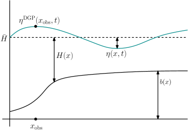
Figure 1: Illustration of the bathymetry $b(x)$, mean fluid depth $H(x)$, surface height perturbation $\eta(x,t)$, and the observation system.

We also consider the linearised version of (1), which ignores second-order terms and assumes that $\eta\ll H$. This gives

$$\begin{cases}u_{t}-\nu u_{xx}+g\eta_{x}=0,&x\in[0,10000],\\ \eta_{t}+\left(Hu\right)_{x}=0,&x\in[0,10000],\\ u(10000,t)=0,\;\eta(0,t)=\tau(t).\end{cases}$$ (4)

Initial conditions, bathymetry, and tidal forcing are the same as those for the fully nonlinear system.

To reconcile the model with observed data we begin by introducing uncertainty into the governing equations (i.e., (1) or (4)) through additive GP forcing, following statFEM. This derives a prior distribution which forms the reference measure for posterior inference. For the nonlinear case this is

$$\begin{cases}u_{t}+uu_{x}-\nu u_{xx}+g\eta_{x}=\xi_{u},&x\in[0,10000],\\ \eta_{t}+\left((H+\eta)u\right)_{x}=\xi_{\eta},&x\in[0,10000],\\ u(10000,t)=0,\;\eta(0,t)=\tau(t).\end{cases}$$ (5)

The linear case follows similarly and is detailed in Appendix B. The a priori uncorrelated GP forcing terms $\xi_{u}$ and $\xi_{\eta}$ are given by

$$\begin{pmatrix}\xi_{u}\\ \xi_{\eta}\end{pmatrix}\sim{\mathcal{GP}}\left(\begin{pmatrix}0\\ 0\end{pmatrix},\delta(t-t^{\prime})\begin{bmatrix}k_{u}(\cdot,\cdot)&0\\ 0&k_{\eta}(\cdot,\cdot)\end{bmatrix}\right).$$

The kernels $k_{u}(\cdot,\cdot)$ and $k_{\eta}(\cdot,\cdot)$ have hyperparameters $\boldsymbol{\Theta}$ which in this work are fixed and known. Estimation methods are available (see, e.g., Williams and Rasmussen, 2006), but we choose to fix parameters for consistency across comparisons, as, in this work, we are interested only in the posterior statFEM filtering inference — not in joint filtering and hyperparameter inference. We use the squared-exponential kernel, given by $k({\mathbf{x}},{\mathbf{x}}^{\prime})=\rho^{2}\exp(-\lVert{\mathbf{x}}-{\mathbf{x}}^{\prime}\rVert^{2}/(2\ell^{2}))$, which we notationally subscript to represent the individual component kernels $k_{u}(\cdot,\cdot)$ and $k_{\eta}(\cdot,\cdot)$, with hyperparameters $\boldsymbol{\Theta}=\{\boldsymbol{\Theta}_{u},\boldsymbol{\Theta}_{\eta}\}=\{\rho_{u},\ell_{u},\rho_{\eta},\ell_{\eta}\}$.

Discretisation of this system now proceeds via the finite element method (FEM) to give a finite-dimensional approximation to the prior. To do so we use the discretisation of Jacobs and Piggott (2015). We use a uniform mesh ${\mathcal{D}}_{h}\subseteq{\mathcal{D}}$ with vertices $\{x_{j}\}_{j=1}^{n_{v}}$; the subinterval length is $h$. We use the $P2$-$P1$ element pair to discretise the state, giving the basis function expansions of $u(x,t)\approx u_{h}(x,t)=\sum_{i=1}^{n_{u}}u_{i}(t)\phi_{i}(x)$, $\eta(x,t)\approx\eta_{h}(x,t)=\sum_{i=1}^{n_{\eta}}\eta_{i}(t)\psi_{i}(x)$. The span of the basis functions $\{\phi_{i}\}_{i=1}^{n_{u}}$ and $\{\psi_{i}\}_{i=1}^{n_{\eta}}$ defines the FEM trial and test spaces for the velocity and surface height perturbations, respectively. The weak form of (5) is given by multiplying by testing functions $(v_{u},v_{\eta})$ and integrating over the spatial domain ${\mathcal{D}}$

$$\langle u_{t},v_{u}\rangle+\langle uu_{x}\rangle+\nu\langle u_{x},v_{u,x}\rangle+g\langle\eta_{x},v_{u}\rangle=\langle\xi_{u},v_{u}\rangle,$$

$$\langle\eta_{t},v_{\eta}\rangle+\langle\left((H+\eta)u\right)_{x},v_{\eta}\rangle=\langle\xi_{\eta},v_{\eta}\rangle,$$

where $\langle f,g\rangle=\int_{\mathcal{D}}fg\,\,{\mathrm{d}}x$. Substituting the finite-dimensional FEM approximations to both the trial and test functions gives differential equations over the FEM coefficients ${\mathbf{u}}=(u_{1},\ldots,u_{n_{u}})$, $\boldsymbol{\eta}=(\eta_{1},\ldots,\eta_{n_{\eta}})$:

$${\mathbf{M}}_{u}\frac{\partial{\mathbf{u}}}{\partial t}+{\mathcal{F}}_{u}({\mathbf{u}})+\nu{\mathbf{A}}{\mathbf{u}}+g{\mathbf{B}}\boldsymbol{\eta}=\boldsymbol{\xi}_{u},$$

$${\mathbf{M}}_{\eta}\frac{\partial\boldsymbol{\eta}}{\partial t}+{\mathcal{F}}_{\eta}({\mathbf{u}},\boldsymbol{\eta})=\boldsymbol{\xi}_{\eta},$$

where ${\mathbf{M}}_{u,ji}=\langle\phi_{i},\phi_{j}\rangle$, ${\mathbf{A}}_{ji}=\langle\phi_{i,x},\phi_{j,x}\rangle$, ${\mathbf{B}}_{ji}=\langle\psi_{i,x},\phi_{j}\rangle$, and ${\mathcal{F}}_{u}(\cdot)$, ${\mathcal{F}}_{\eta}(\cdot,\cdot)$ are functions which result from discretising the nonlinear operators.

The FEM discretised GP forcing terms, $\boldsymbol{\xi}_{u}$ and $\boldsymbol{\xi}_{\eta}$, are given by the approximation $\boldsymbol{\xi}\sim{\mathcal{N}}({\mathbf{0}},{\mathbf{M}}{\mathbf{K}}{\mathbf{M}}^{\top})$, where ${\mathbf{K}}_{ij}=k(x_{i},x_{j})$, for nodal $x_{i}$, $x_{j}$ (Duffin et al., 2021) (note omitted subscripts are for readability). This approximation uses different mass matrices ${\mathbf{M}}$ across components due to the components $u$ and $\eta$ using different basis functions for the FEM approximation. Thus we have, jointly, $(\boldsymbol{\xi}_{u},\boldsymbol{\xi}_{\eta})\sim{\mathcal{GP}}({\mathbf{0}},\delta(t-t^{\prime}){\mathbf{G}})$, where ${\mathbf{G}}$ has the block-diagonal structure:

$${\mathbf{G}}=\begin{bmatrix}{\mathbf{M}}_{u}{\mathbf{K}}_{u}{\mathbf{M}}_{u}^{\top}&{\mathbf{0}}\\ {\mathbf{0}}&{\mathbf{M}}_{\eta}{\mathbf{K}}_{\eta}{\mathbf{M}}_{\eta}^{\top}\end{bmatrix}.$$

A low-rank approximation is required, in order to run our filtering methodology (Duffin et al., 2022). To get a low-rank approximation of this covariance matrix we make use of the block structure. Using the factorisation ${\mathbf{G}}={\mathbf{G}}^{1/2}{\mathbf{G}}^{\top/2}$, we approximate

$${\mathbf{G}}^{1/2}\approx\begin{bmatrix}{\mathbf{M}}_{u}{\mathbf{K}}_{u}^{1/2}&{\mathbf{0}}\\ {\mathbf{0}}&{\mathbf{M}}_{\eta}{\mathbf{K}}_{\eta}^{1/2}\end{bmatrix},$$

where ${\mathbf{K}}_{u}^{1/2}\in{\mathbb{R}}^{n_{u}\times q_{u}}$ and ${\mathbf{K}}_{\eta}^{1/2}\in{\mathbb{R}}^{n_{\eta}\times q_{\eta}}$, for $q_{u}\ll n_{u}$, $q_{\eta}\ll n_{\eta}$. The block-structured low-rank approximation gives $(\boldsymbol{\xi}_{u},\boldsymbol{\xi}_{\eta})^{\top}\sim{\mathcal{GP}}({\mathbf{0}},\delta(t-t^{\prime}){\mathbf{G}}^{1/2}{\mathbf{G}}^{\top/2})$, where ${\mathbf{G}}^{1/2}\in{\mathbb{R}}^{(n_{u}+n_{\eta})\times(q_{u}+q_{\eta})}$. Approximations can be computed through e.g., GPU computing (Charlier et al., 2021) or Nyström approximation (Williams and Seeger, 2001), but in this work we use the Hilbert-GP approach of Solin and Särkkä (2020). This enforces that the additive GPs should be zero on the boundaries. It was found empirically that our GP approximations needed to respect zero boundary conditions or otherwise the posterior covariance would be overly uncertain on the edges of the domain, leading to poor numerical approximation of the covariance.

To discretise the dynamics in time we use the $\theta$-method (Hairer et al., 1993) for stability. Letting ${\mathbf{u}}^{n}:={\mathbf{u}}(n{\Delta_{t}})$ and $\boldsymbol{\eta}^{n}:=\boldsymbol{\eta}(n{\Delta_{t}})$, the time-discretised stochastic dynamics are

$${\mathbf{M}}_{u}\frac{{\mathbf{u}}^{n}-{\mathbf{u}}^{n-1}}{{\Delta_{t}}}+{\mathcal{F}}_{u}({\mathbf{u}}^{n-\theta})\\ +\nu{\mathbf{A}}{\mathbf{u}}^{n-\theta}+g{\mathbf{B}}\boldsymbol{\eta}^{n-\theta}=\frac{1}{\sqrt{{\Delta_{t}}}}\boldsymbol{\xi}_{u}^{n-1},\\ {\mathbf{M}}_{\eta}\frac{\boldsymbol{\eta}^{n}-\boldsymbol{\eta}^{n-1}}{{\Delta_{t}}}+{\mathcal{F}}_{\eta}({\mathbf{u}},\boldsymbol{\eta}^{n-\theta})=\frac{1}{\sqrt{{\Delta_{t}}}}\boldsymbol{\xi}_{\eta}^{n-1},$$

where ${\mathbf{u}}^{n-\theta}:=\theta{\mathbf{u}}^{n}+(1-\theta){\mathbf{u}}^{n-1}$ (similarly for $\boldsymbol{\eta}$), for $\theta\in[0,1]$. The initial conditions $({\mathbf{u}}^{0},\boldsymbol{\eta}^{0})$ are known so we begin by solving for $({\mathbf{u}}^{1},\boldsymbol{\eta}^{1})$. Running the scheme gives the entire set of states $\{({\mathbf{u}}^{n},\boldsymbol{\eta}^{n})\}_{n=0}^{N}$ so that $N{\Delta_{t}}=T$.

Observations may also be arriving at particular timepoints, and we want to condition on these observations to get an a posteriori estimate of the state. We assume that the time between observations is $k{\Delta_{t}}$, for some integer $k\geq 1$, giving the observations as ${\mathbf{y}}_{m}:={\mathbf{y}}(mk{\Delta_{t}})$, and the total set of observations $\{{\mathbf{y}}_{m}\}_{m=1}^{M}$ — the initial state $({\mathbf{u}}^{n},\boldsymbol{\eta}^{n})$ is always assumed known. This ensures $\{mk{\Delta_{t}}\}_{m=1}^{M}\subset\{n{\Delta_{t}}\}_{n=0}^{N}$ and thus $M\leq N$.

The joint dynamics and observation model is to take $k$ model steps, thus for $n=(m-1)k,\ldots,mk$ we predict using the model:

$$\begin{gathered}{\mathbf{M}}_{u}\frac{{\mathbf{u}}^{n}-{\mathbf{u}}^{n-1}}{{\Delta_{t}}}+{\mathcal{F}}_{u}({\mathbf{u}}^{n-\theta})\\ \qquad\qquad\qquad\quad+\nu{\mathbf{A}}{\mathbf{u}}^{n-\theta}+g{\mathbf{B}}\boldsymbol{\eta}^{n-\theta}=\frac{1}{\sqrt{{\Delta_{t}}}}\boldsymbol{\xi}_{u}^{n-1},\\ {\mathbf{M}}_{\eta}\frac{\boldsymbol{\eta}^{n}-\boldsymbol{\eta}^{n-1}}{{\Delta_{t}}}+{\mathcal{F}}_{\eta}({\mathbf{u}},\boldsymbol{\eta}^{n-\theta})=\frac{1}{\sqrt{{\Delta_{t}}}}\boldsymbol{\xi}_{\eta}^{n-1}.\end{gathered}$$ (6)

We abbreviate this by writing the l.h.s. of (6) as ${\mathcal{M}}:{\mathbb{R}}^{(n_{u}+n_{\eta})\times 2}\to{\mathbb{R}}^{n_{u}+n_{\eta}}$, with Jacobian matrix ${\mathbf{J}}_{n}$.

At the observation timepoint $mk{\Delta_{t}}$ we condition on the data

$${\mathbf{y}}_{m}={\mathbf{H}}({\mathbf{u}}_{m},\boldsymbol{\eta}_{m})+{\mathbf{r}}_{m},$$

where $({\mathbf{u}}_{m},\boldsymbol{\eta}_{m})=({\mathbf{u}}^{mk},\boldsymbol{\eta}^{mk})$ and ${\mathbf{r}}_{m}\sim{\mathcal{N}}({\mathbf{0}},{\mathbf{R}})$. The linear observation operator ${\mathbf{H}}:{\mathbb{R}}^{n_{u}+n_{\eta}}\to{\mathbb{R}}^{n_{y}}$ is known a priori. In this work, it is given by the FEM polynomial interpolants. To condition on the observations we use the low-rank extended Kalman filter (LR-ExKF)— a recursive two-step scheme consisting of prediction and update steps. At timesteps which are not observed only the model prediction steps are completed. This computes the approximation $p({\mathbf{u}}_{m},\boldsymbol{\eta}_{m}\>|\>{\mathbf{y}}_{1:m},\boldsymbol{\Theta},\nu,c)\sim{\mathcal{N}}(\boldsymbol{\mu}_{m},{\mathbf{L}}_{m}{\mathbf{L}}_{m}^{\top})$, a multivariate Gaussian over the concatenation of $({\mathbf{u}}_{m},\boldsymbol{\eta}_{m})$, an $n_{u}+n_{\eta}$ dimensional object. For a rank-$q$ approximation to the covariance matrix we thus have ${\mathbf{L}}_{m}\in{\mathbb{R}}^{(n_{u}+n_{\eta})\times q}$. For a single prediction-update cycle, the algorithm is shown in Algorithm 1.

$\boldsymbol{\mu}_{m-1}$, ${\mathbf{L}}_{m-1}$, such that $({\mathbf{u}}_{m-1},\boldsymbol{\eta}_{m-1}\>|\>\boldsymbol{\Theta},\nu,c)\sim{\mathcal{N}}(\boldsymbol{\mu}_{m-1},{\mathbf{L}}_{m-1}{\mathbf{L}}_{m-1}^{\top})$.

Let $\boldsymbol{\mu}^{n}\equiv\boldsymbol{\mu}_{m-1}$, ${\mathbf{L}}^{n}\equiv{\mathbf{L}}_{m-1}$.

for $(m-1)k<n\leq mk$ do

     Solve ${\mathcal{M}}(\boldsymbol{\mu}^{n},\boldsymbol{\mu}^{n-1})={\mathbf{0}}$, for $\boldsymbol{\mu}^{n}$.

     $\tilde{\mathbf{L}}^{n}=\left[{\mathbf{J}}_{n}^{-1}{\mathbf{J}}_{n-1}{\mathbf{L}}_{n-1},\;{\mathbf{J}}_{n}^{-1}{\mathbf{G}}^{1/2}\right]$.

     Eigendecomposition: ${\mathbf{V}}_{n}\boldsymbol{\Sigma}_{n}{\mathbf{V}}_{n}^{\top}=({\tilde{\mathbf{L}}}^{n})^{\top}\tilde{\mathbf{L}}^{n}$.

     ${\mathbf{L}}^{n}=\tilde{\mathbf{L}}^{n}[{\mathbf{V}}]_{:,1:q}$.

end for

$\boldsymbol{\mu}^{n}\leftarrow\boldsymbol{\mu}^{n}+{\mathbf{L}}^{n}({\mathbf{H}}{\mathbf{L}}^{n})^{\top}({\mathbf{H}}{\mathbf{L}}^{n}({\mathbf{H}}{\mathbf{L}}^{n})^{\top}+\sigma^{2}{\mathbf{I}})^{-1}({\mathbf{y}}_{m}-{\mathbf{H}}\boldsymbol{\mu}^{n})$.

Cholesky decomposition: ${\mathbf{R}}_{n}{\mathbf{R}}_{n}^{\top}={\mathbf{I}}-({\mathbf{H}}{\mathbf{L}}^{n})^{\top}({\mathbf{H}}{\mathbf{L}}^{n}({\mathbf{H}}{\mathbf{L}}^{n})^{\top}+\sigma^{2}{\mathbf{I}})^{-1}{\mathbf{H}}{\mathbf{L}}^{n}$.

${\mathbf{L}}^{n}\leftarrow{\mathbf{L}}^{n}{\mathbf{R}}_{n}$.

return $\boldsymbol{\mu}_{m}\equiv\boldsymbol{\mu}^{n}$, ${\mathbf{L}}_{m}\equiv{\mathbf{L}}^{n}$.

Algorithm 1 Prediction-update cycle of the LR-ExKF algorithm (rank $q$).

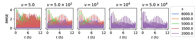
Figure 2: Prior statFEM RMSE: computed for models with $s\in\{2000,3500,5000,6500,8000\}$ and $\nu\in\{5,500,10^{3},10^{4},5\times 10^{4}\}$, every $30$ s.

3 Experimental setup

To generate the synthetic dataset, $\{{\mathbf{y}}_{m}\}_{m=1}^{M}$, we use the FEM discretisation of the fully nonlinear SWE (of Equation (1)) as detailed above for the statFEM model. That is, we use the same $P2$-$P1$ basis function pairs to give the FEM discretised approximations $(u_{h}^{\mathrm{DGP}}(x,t),\eta_{h}^{\mathrm{DGP}}(x,t))$. These are computed using a uniform mesh with $n_{v}=500$ elements ($h=20$ $\mathrm{m}$), and timesteps of size ${\Delta_{t}}=1$ $\mathrm{s}$. We set $\theta=0.6$. Observations are given by

$${\mathbf{y}}_{m}=\boldsymbol{\eta}_{m}^{\mathrm{obs}}+{\mathbf{r}}_{m},\\ \boldsymbol{\eta}_{m}^{\mathrm{obs}}:=\left(\eta_{h}^{\mathrm{DGP}}(x_{1}^{\mathrm{obs}},mk{\Delta_{t}}),\ldots,\eta_{h}^{\mathrm{DGP}}(x_{n_{y}}^{\mathrm{obs}},mk{\Delta_{t}})\right)^{\top},$$

where the i.i.d. noise is ${\mathbf{r}}_{m}\sim{\mathcal{N}}({\mathbf{0}},\sigma^{2}{\mathbf{I}})$, with $\sigma=5\times 10^{-2}$. This data is generated with $\nu=1$, and the shore position is $s=2000$. We take $n_{y}$ observations per observed time point, the locations of which are uniformly spaced between in the interval $[1000,2000]$ $\mathrm{m}$. Note that when $n_{y}=1$ this corresponds to observing at $x_{\mathrm{obs}}=1000$ $\mathrm{m}$.

Our experiments compare results a priori with results a posteriori under different model configurations to those used to generate the data. The posterior distribution is given by $p({\mathbf{u}}_{m},\boldsymbol{\eta}_{m}\>|\>{\mathbf{y}}_{1:m},\boldsymbol{\Theta},\sigma,\nu,c)$, which we compute an approximation to using the LR-ExKF. The posterior $(u_{h},\eta_{h})$ is computed using the same numerical settings as for the data. The observation operator ${\mathbf{H}}$ is defined via

$${\mathbf{H}}({\mathbf{u}}_{m},\boldsymbol{\eta}_{m}):=\\ \left(\eta_{h}(x_{1}^{\mathrm{obs}},mk{\Delta_{t}}),\ldots,\eta_{h}(x_{n_{y}}^{\mathrm{obs}},mk{\Delta_{t}})\right)^{\top},$$

and we assume that the noise level $\sigma$ is known, simulating the scenario of known measurement device error. We compute the posterior distribution across a Cartesian product of the different input parameters, with $k\in\{1,30,60,120,180\}$, $n_{y}\in\{1,2,5\}$, $s\in\{2000,3500,5000,6500,8000\}$, and $\nu\in\{5,500,1000,10000,50000\}$. Across the nonlinear and linear models this gives $750$ different configurations. Note that we do not estimate the statFEM posterior for $\nu=1$ due to numerical instabilities when computing the posterior covariance, however results were similar to that with $\nu=5$, which is reported here. For the stochastic GP forcing, we set $\ell_{u}=\ell_{\eta}=1000$, $\rho_{u}=0$, and $\rho_{\eta}=2\times 10^{-3}$. The magnitudes of $\rho_{u}$ and $\rho_{\eta}$ are chosen to balance between accurate UQ when estimating a well-specified model, and adequate uncertainty when estimating a poorly specified model.

To get a feel for model performance a priori — and hence the severity of model misspecification — we estimate the prior distribution for the nonlinear model, $p({\mathbf{u}}_{m},\boldsymbol{\eta}_{m}\>|\>\nu,s,\boldsymbol{\Theta})\sim{\mathcal{N}}(\boldsymbol{\mu}_{m},{\mathbf{L}}_{m}{\mathbf{L}}_{m}^{\top})$, across the grid of $s$ and $\nu$ values. This is done through running the filter with the prediction steps only, for all timesteps. To compare with the data we compute the root-mean-square error (RMSE). The RMSE is

$${\mathrm{RMSE}}_{m}=\frac{\lVert{\mathbf{y}}_{m}-{\mathbf{H}}\boldsymbol{\mu}_{m}\rVert_{2}}{\sqrt{n_{y}}},$$ (7)

where $\lVert\cdot\rVert_{2}$ is the Euclidean $l^{2}$ norm. Results are shown in Figure 2. For $\nu=5$ there is a clear stratification between the well-specified $s=2000$ model and the others which are misspecified. The errors in these models appear to lack the consistent periodicity that models with larger $\nu$ see. In these cases we see that there is a consistently large error across each model with no synchronicity across the systems. The stratification between these models becomes less apparent as $\nu$ increases up to $5\times 10^{4}$, a result of the dissipative effects dominating the dynamics. This leads to models with different $s$ performing similarly as the wave profiles dissipate the energy input from the tidal forcing.

There emerges a periodicity across the solutions as $\nu$ increases, thought to be due to the tidal forcing. We see that there is a sharp increase in early times, then a similar increase approximately in the middle of the time domain. This increase is thought to be due to the cycle of the forcing starting to “swing down” into the lower cycle of the tidal forcing. We note also that there are similar timescales in the error dynamics and no models appear to dissipate to equilibrium — again due to the oscillatory forcing.

4 Results

In this section we analyse the posterior results. First, we conduct a preliminary analysis of the model posteriors, to give intuition on how our chosen metrics relate to the posterior distribution. Next, we analyse how the observation frequencies $k$ and $n_{y}$ effect the posterior distribution in the face of misspecification. We then study the case of joint viscosity-bathymetry misspecification, and then conclude with the analysis of the linearised model, also under joint viscosity-bathymetry misspecification.

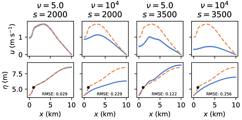
(a) Observations, posterior means and $0.95$ probability intervals, at time $t=11.67$ $\mathrm{h}$. Average RMSE is shown within each plot, and the truth is shown in orange (   ).

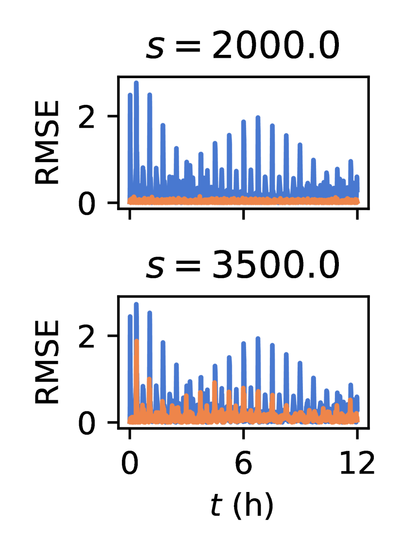
(b) RMSE: $\nu=5$ shown in orange ( ) and $\nu=10^{4}$ shown in blue ( ).

Figure 3: Posterior means and variances (3(a)), and posterior RMSE values (3(b)) for the nonlinear models with $s\in\{2000,3500\}$ $\mathrm{m}$, $\nu\in\{5,10^{4}\}$ $\mathrm{m}^{2}\mathrm{/}\mathrm{s}$.

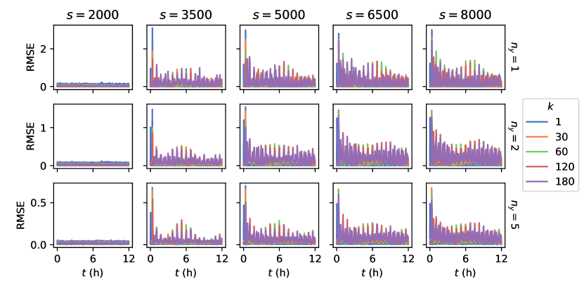
(a) RMSE values across time, across different $s$, $n_{y}$, and $k$ ($\nu=5$).

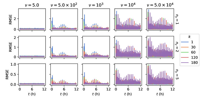
(b) RMSE values across time as $\nu$, $n_{y}$, and $k$ are varied ($s=2000$).

Figure 4: Observation frequency: posterior RMSE values, across time, for the models as observation frequency is varied.

4.1 Preliminary analysis of posterior distributions

To get a feel for the posterior results we now describe the results for four models. Each have observations arriving every $k=30$ timesteps (every $30$ $\mathrm{s}$). We run the nonlinear model with $s\in\{2000,3500\}$ and $\nu\in\{5,10^{4}\}$.

At time $t=11.67$ $\mathrm{h}$ we have plotted the posterior means and variances in Figure 3(a). The well specified model captures the more complex dynamical behaviour well with a notable improvement in the estimation of the velocity fields, in comparison to the other models. The more damped models, with $\nu=10^{4}$, appear unsurprisingly to underestimate the data at this observation point. Due to the right-shifted bathymetry an increase in velocity is seen to the right of the observation location when $s=3500$, $\nu=5$. The velocity fields are all underestimated, with a notably poor-performing case with $s=3500$ $\mathrm{m}$ and $\nu=10^{4}$. In this case the data (observed only on the surface height perturbation) can only correct for so much, and the dynamics must also be appropriately specified in order for the model to be accurate. We also see that the uncertainty on $\eta$ has given rise to uncertainty in $u$ following intuition; a posteriori it is seen that the unobserved velocity components have increased uncertainty.

As introduced above, to quantitatively compare performance we use the RMSE. For the models introduced above the average values of these, across all time, are shown within the second row in Figure 3(a). Across the variations in RMSE there is a qualitative stratification which is especially apparent on the unobserved velocity components. The RMSEs are plotted across time in Figure 3(b); similar stratification is seen to that in Figure 3(a). Variation is seen across the models as data is conditioned on; this is most clearly observed with the poorly performing high-viscosity models. The low-viscosity model with $\nu=5$ performs well. The mildly-misspecified $\{\nu=5,s=3500\}$ performs moderately well and improves upon the prior (see Figure 2).

4.2 Investigating observation frequency

In the second simulation study we study the model performance as we vary the observation frequency in space and time, taking $n_{y}\in\{1,2,5\}$ and $k\in\{1,30,60,120,180\}$, whilst also varying the topography and viscosity.

First, we look at the case of a well-specified viscosity ($\nu=5$), with misspecified bathymetry, with $s\in\{2000,3500,5000,6500,8000\}$. In Figure 4(a) we plot the RMSE values over all the observed timepoints, for each model. Increasing $n_{y}$ decreases the model error across all models. Similar reductions in the RMSE are not seen with the increase of $k$. Whilst there are improvements, especially for all $k=1$, and $n_{y}=1$, it is seen otherwise that the observation frequency $k$ does not have the same drastic effect.

We next look at the case of a well-specified $s=2000$ and a variable viscosity $\nu\in\{5,500,10^{3},10^{4},5\times 10^{4}\}$. Results when varying $\nu$ are shown in Figure 4(b). For $\nu\leq 10^{3}$ we see that the models perform relatively well; conditioning on data ensures that the misspecification induced through the viscosity is corrected for. As $\nu$ increases we see the regular increase in error, through the middle of simulation time (at $t\approx 6$ $\mathrm{h}$). Whilst the RMSE values vary magnitude-wise, this regular quasi-periodic structure emerges across each of the models. This approximately corresponds to the tidal forcing $\tau(t)$ hitting its minimum through the simulation (Figure 5). Errors decrease as this forcing begins to increase once again.

Increasing the observation density in space again results in a marked improvement in model discrepancy. As previous with $k=1$ this results in the most notable improvement in the RMSE, with mild improvements for $k\geq 30$. As $\nu\geq 10^{4}$, there is no visual distinction between the models with such high viscosities. Error due to the topography appears to result in a greater degree of stratification between each of the models. This is unsurprising as whilst misspecifying the viscosity leads to mismatch, beyond $\nu=10^{4}$ the viscous effects dominate the flow, resulting in similar behaviour.

	1	30	60	120	180
1	0.0543 (0.080)	0.1222 (0.123)	0.1447 (0.128)	0.1792 (0.153)	0.1944 (0.177)
2	0.0417 (0.048)	0.0720 (0.073)	0.0857 (0.072)	0.1019 (0.080)	0.1127 (0.079)
5	0.0266 (0.026)	0.0356 (0.040)	0.0389 (0.042)	0.0438 (0.045)	0.0452 (0.027)

Table 2: Mean RMSE values and standard deviations (in parentheses) for the nonlinear statFEM SWE model, as the observation frequency is changed, with mild misspecification: $s=3500$ and $\nu=5$.

For a single instance of “mild misspecification” with $s=3500$ and $\nu=5$, the empirical means and standard deviations (computed across time) of their RMSEs are shown in Table 2. As more spatial locations are observed, the frequency of observations in time has less of an effect on the accuracy of the model. When observing $n_{y}=5$ locations, small increases in the RMSE are seen with less frequent observations in time. These increases are notably larger when taking $n_{y}=1$. An interesting result is that increasing $n_{y}$ from $1$ to $5$ results in improved performance, even when observing every $180$ $\mathrm{s}$. The inclusion of additional spatial measurement locations results in a dramatic improvement in the performance of the model. This is thought to be due to the fact that the flow in this case has a long wavelength — incorporating data over a larger spatial domain therefore has a more corrective effect on the model as it is now observed over a set of spatiotemporal locations.

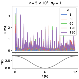
Figure 5: RMSE and tidal forcing $\tau(t)$ with $\nu=5\times 10^{4}$ and $n_{y}=1$. Errors increase when the forcing is at its minimum.

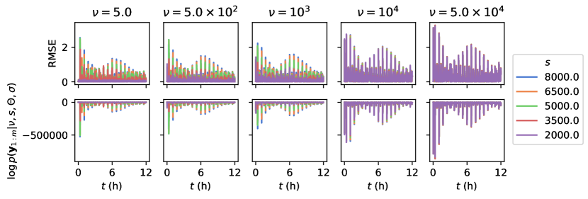
Figure 6: Posterior bathymetry-viscosity misspecification. RMSE values as $\nu$ and $c$ are varied (top), and negative log-likelihood values (bottom), for fixed observation interval $k=100$.

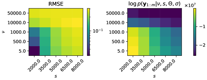
Figure 7: Color table of RMSE and negative log-likelihood results as $s$ and $\nu$ are varied. For numeric comparisons with the above figures, the RMSE is averaged across all observation times.

	2000.0	3500.0	5000.0	6500.0	8000.0
5	$\mathbf{-1.541\times 10^{5}}$	$\mathbf{-3.453\times 10^{6}}$	$\mathbf{-8.174\times 10^{6}}$	$\mathbf{-1.180\times 10^{7}}$	$\mathbf{-1.406\times 10^{7}}$
500	$-8.184\times 10^{5}$	$-3.599\times 10^{6}$	$-9.216\times 10^{6}$	$-1.346\times 10^{7}$	$-1.582\times 10^{7}$
1000	$-1.795\times 10^{6}$	$-4.249\times 10^{6}$	$-9.866\times 10^{6}$	$-1.441\times 10^{7}$	$-1.701\times 10^{7}$
10000	$-1.736\times 10^{7}$	$-1.855\times 10^{7}$	$-2.091\times 10^{7}$	$-2.284\times 10^{7}$	$-2.403\times 10^{7}$
50000	$-2.409\times 10^{7}$	$-2.541\times 10^{7}$	$-2.562\times 10^{7}$	$-2.564\times 10^{7}$	$-2.564\times 10^{7}$

Table 3: Table of log-likelihoods as $\nu$ and $s$ are varied. Minimums for each column are highlighted in bold.

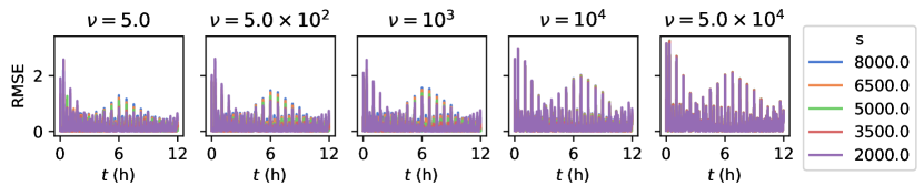
Figure 8: RMSE across time for the linear model, as $\nu$ and $s$ are varied.

	2000.0	3500.0	5000.0	6500.0	8000.0
5	$\mathbf{-7.778\times 10^{6}}$	$\mathbf{-6.234\times 10^{6}}$	$\mathbf{-6.235\times 10^{6}}$	$\mathbf{-7.137\times 10^{6}}$	$\mathbf{-9.580\times 10^{6}}$
500	$-8.476\times 10^{6}$	$-6.901\times 10^{6}$	$-7.221\times 10^{6}$	$-8.630\times 10^{6}$	$-1.075\times 10^{7}$
1000	$-9.182\times 10^{6}$	$-7.653\times 10^{6}$	$-8.136\times 10^{6}$	$-9.662\times 10^{6}$	$-1.166\times 10^{7}$
10000	$-1.790\times 10^{7}$	$-1.734\times 10^{7}$	$-1.781\times 10^{7}$	$-1.856\times 10^{7}$	$-1.914\times 10^{7}$
50000	$-2.219\times 10^{7}$	$-2.337\times 10^{7}$	$-2.361\times 10^{7}$	$-2.360\times 10^{7}$	$-2.357\times 10^{7}$

Table 4: Linear misspecification: table of log-likelihoods, as $\nu$ and $s$ are varied, for fixed spatiotemporal observation frequencies.

4.3 Investigating parametric misspecification

Following these results, we now investigate joint parametric misspecification of $s\in\{2000,3500,5000,6500,8000\}$ and $\nu\in\{5,500,10^{3},10^{4},5\times 10^{4}\}$. We set $n_{y}=1$, and $k=30$ ($1$ spatial location observed every $30$ $\mathrm{s}$). In Figure 6 (top) the RMSE is shown for the estimated posterior distributions $p({\mathbf{u}}_{m},\boldsymbol{\eta}_{m}\>|\>{\mathbf{y}}_{1:m},\nu,s,\boldsymbol{\Theta},\sigma)$. As previous we see that the models with small $\nu$ are more accurate. Additionally, as $s$ is increasingly misspecified there is a stratification of model performance, with, unsurprisingly, the correctly specified $s=2000$ quite noticeably out-performing the misspecified models. With larger $\nu$ values we see that there is a mild increase in the RMSE through conditioning on data. Less stratification appears to be present as $\nu$ is increased; damping dominates the misspecified bathymetry in terms of mismatch.

For additional model comparison, we use the log-likelihood. Due to the structure of this problem we can write this via factorisation

$$\log p({\mathbf{y}}_{1:M}\>|\>\nu,s,\boldsymbol{\Theta},\sigma)=\\ \log p({\mathbf{y}}_{1}\>|\>\nu,s,\boldsymbol{\Theta},\sigma)\\ +\sum_{m=2}^{M}\log p({\mathbf{y}}_{m}\>|\>{\mathbf{y}}_{1:m-1},\nu,s,\boldsymbol{\Theta},\sigma).$$

This can be approximated when running the LR-ExKF, due to the Gaussian approximation. The individual likelihoods are of the form

$$p({\mathbf{y}}_{m}\>|\>{\mathbf{y}}_{1:m-1},\nu,s,\boldsymbol{\Theta},\sigma)=\\ ={\mathcal{N}}({\mathbf{H}}\hat{\boldsymbol{\mu}}_{m},({\mathbf{H}}\hat{{\mathbf{L}}}_{m})({\mathbf{H}}\hat{{\mathbf{L}}}_{m})^{\top}+\sigma^{2}{\mathbf{I}}),$$

where $p({\mathbf{u}}_{m}\>|\>{\mathbf{y}}_{1:m-1},\nu,s,\boldsymbol{\Theta},\sigma)={\mathcal{N}}(\hat{\boldsymbol{\mu}}_{m},\hat{{\mathbf{L}}}_{m}\hat{{\mathbf{L}}}_{m}^{\top})$. This is a strictly proper scoring rule with respect to Gaussian measure (Gneiting and Raftery, 2007). Intuitively, this is an uncertainty-weighted scoring rule that punishes models which are more certain about inaccurate predictions of the data, at each observation time.

The log-likelihoods are shown, across time, in Figure 6. The models stratify across $s$ more obviously for the well-specified models, with less stratification as $\nu$ is increased. All models show a gradual decrease in the log-likelihood values over time; conditioning on data results in more accurate models. Note also that similar to the RMSE values (see also Figure 5) we see that there is the same quasi-periodic behaviour as the tidal forcing begins to approach $0$, resulting in decreases in the likelihood.

For visual comparison, the average RMSE values and the log-likelihoods are shown in Figure 7. As previous, we see that with $\nu\geq 10^{4}$ there is a clear increase in the RMSE marking a qualitative change in the dynamics. Similar model stratification is seen for the RMSE as is for the log-likelihood; in these examples they perform similarly as model comparison metrics. These log-likelihoods are tabulated in Table 3. Models with $\nu=5$ are preferred across each bathymetry.

Following the computations of the log-likelihoods, we can perform model comparison via Bayes factors (Kass and Raftery, 1995). The Bayes factor is given by the ratio of the probabilities of the data given the different assumed models:

$$\log{\mathrm{BF}}_{10}=\log p({\mathbf{y}}_{1:M}\>|\>\nu_{1},s_{1},\boldsymbol{\Theta},\sigma)\\ -\log p({\mathbf{y}}_{1:M}\>|\>\nu_{0},s_{0},\boldsymbol{\Theta},\sigma).$$ (8)

We see that there is strong evidence in favour of the well-specified model in comparison to the others (smallest $\log{\mathrm{BF}}_{10}\approx 10^{5}$). In each case it is clear that increasing the degree of misspecification, by either shifting the topography, or, increasing the misspecification, results in less performant models. Models with smaller $\nu$ are preferred over those which have a larger $\nu$. Interestingly, there is very strong evidence against the model with $\{\nu=5\times 10^{4},s=2000\}$, in comparison with that of $\{\nu=5,s=8000\}$ ($\log{\mathrm{BF}}_{10}\approx 10^{7}$). We notice that the trend misspecification due to $s$ tends to be less severe than that due to $\nu$ (see also Figure 7).

4.4 Linearisation

Finally we investigate joint viscosity-bathymetry misspecification as in the previous subsection, with the addition of model linearisation. As previous, we vary $s\in\{2000,3500,5000,6500,8000\}$ and $\nu\in\{5,500,10^{3},10^{4},5\times 10^{4}\}$, whilst fixing $k=30$ and $n_{y}=1$ to compute the posterior estimates. We plot the RMSE values across time for these linearised model approximations in Figure 8. The RMSE values, in comparison to those of the nonlinear models, are slightly larger with notable increases in the cases of well-specified bathymetry.

This disparity in model performance is further realised in the log-likelihoods (seen in Table 4) being larger for the well-specified models in comparison to those of the poorly specified models. We see the unsurprising results that small-$\nu$ models perform better than the others. In comparing Tables 3 and 4 it is seen that when the severity of model misspecification is larger (approximately $s\geq 5000$, $\nu\geq 10^{4}$) the linear model outperforms the nonlinear model. For $s\geq 5000$ we posit this is due to the ignoring of the resultant interactions between the misspecified bathymetry and velocity. When damping is very highly misspecified, even for a well-specified bathymetry the linear model is preferred. Again this is thought to be due to the addition of nonlinearity not really contributing to the dynamics — in this regime the dynamics are dominated by the linear dissipative behaviour, in any case.

5 Discussion and conclusion

In this work we studied the efficacy of statFEM as applied to the $1D$ SWE, to see how the methodology responds to scenarios of increasing model misspecification. Previous work has necessarily included smaller studies of milder cases of model misspecification; this work provides the first systematic analysis of the approach under gradually increased misspecification severity. Misspecification was induced via linearisation, viscosity, and bottom-topography (bathymetry), in regimes of reduced spatiotemporal observational frequency. The RMSE and log-likelihood were used for model comparison.

The methodology is able to appropriately deal with model misspecification with notably large improvements in model error as the number of observation locations is increased; the method performs well in recovering misspecified dynamics. This is thought to be due to spatial variation being more informative to the model error than increasing the frequency of observations. The changes in observation frequency are small in comparison to the timescale of the flow and thus the differences in the observations, arriving at different times are not large enough to warrant drastic reductions in model error (though there is still a reduction). However, as wavelengths are relatively long the additional information included via spatial variation, through additional observation locations, does indeed result in marked reductions in model error. Note also that our model error term, the GP $\xi$, induces spatial correlations over components of model error. Therefore including additional observation locations, which make use of this error structure is again thought to be helpful. We note that whilst we did not include temporal correlation in $\xi$, a priori, the additional study and comparison of model error structures being correlated in both space and time is of interest.

The effects of misspecification have different qualitative behaviors. When $\nu$ is well-specified the bathymetry parameter $s$ results in immediate increases in error which are of similar magnitude. On the other hand, as noted previously (see also Figure 5) when $\nu$ is misspecified a regular quasi-periodic pattern in the error emerges which results in nearly visually indistinguishable error patterns. We see, also, that due to the domination of the dissipation these periodic-type patterns in the error are also seen in the linear model for lower values of $\nu$. More severe mismatch is seen to result from large dissipation values rather than large shifts of the bottom-topography. Both, however, are reduced through observing more spatial locations. It is worth noting that there is a clear visual decrease in the amount of model error present when taking $n_{y}=2$ instead of $n_{y}=1$ (see Figure 4), when the topography is misspecified. When designing observation systems (i.e. measurement/sensor locations) this suggests that taking additional observation locations is valuable when they are of a similar lengthscale to the flow under consideration. In cases of severe misspecification linear approximations aid in slightly reducing the model error, as seen via the log-likelihoods.

Whilst the RMSE and log-likelihood are useful and theoretically sound metrics, the study of appropriate additional metrics (such as, e.g., the Brier score (Brier, 1950)) would be a useful tool for practitioners when implementing and diagnosing models. We also note that our results are conditioned on sets of GP hyperparameters which, whilst chosen to ensure appropriate UQ on a well-specified model, are not optimal with regards to the log-likelihood. Joint investigation of hyperparameter estimation and filtering is of interest and is a possible avenue of further research.

Model error in this study appears to arrive in similar timescales no matter which parameter is misspecified. In exploring alternate models before we settled on the model used in this paper, we found that there were intuitive interactions between the timescales of model error and posterior updating. When mismatch occurs in fast timescales more frequent updating is preferred. For slow timescales less frequent updating is required.

These results provide additional evidence that the statFEM approach allows for statistically coherent inference in regimes of potentially severe model misspecification. The admission of spatially correlated and physically sensible uncertainty results in improvements in model accuracy as data is assimilated. The induced uncertainty is sensible and reflects modelling choices: for example, boundary conditions are respected and unobserved components are less certain a posteriori. From the statistical point-of-view, the inclusion of physical information alongside the GP enables the use of sparse data. Results suggest that the inclusion of data, irrespective of the amount, only aids in model proficiency when using statFEM.

Appendix A FEM discretisation

To justify the chosen discretisation and level of mesh-refinement, the deterministic FEM convergence results are plotted in Figure 9. We run a reference model $(u_{h}^{\mathrm{ref}},\eta_{h}^{\mathrm{ref}})$ with $n_{v}=3000$ cells, and compute the $L^{2}$ errors against this reference model, after running the models with ${\Delta_{t}}=1$ up to time $t=600$ $\mathrm{s}$ with meshes having $n_{v}\in\{500,600,750,1000,1500\}$. Errors shrink with a cubic rate (est. gradient $3.0144$).

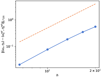
Figure 9: Deterministic FEM convergence for our employed discretisation. Discretisation error is shown as a blue line ( ), and dashed line shown in orange (   ) is for reference, having gradient 3.

Appendix B Notes on linear statFEM

In the linear case, we recall that the statFEM model definition is

$$\begin{cases}u_{t}+g\eta_{x}+\nu u_{xx}=\xi_{u},&x\in{\mathcal{D}},\\ \eta_{t}+\left(Hu\right)_{x}=\xi_{\eta},&x\in{\mathcal{D}},\\ u_{x}=0,\;\eta=0,&x\in\partial{\mathcal{D}}.\end{cases}$$ (9)

As previous we model the forcing terms $\xi_{u}$ and $\xi_{\eta}$ by a priori uncorrelated GPs. Making use of the same $P2$-$P1$ discretisation as previous gives

$${\mathbf{M}}_{u}\frac{{\mathbf{u}}^{n}-{\mathbf{u}}^{n-1}}{{\Delta_{t}}}+\nu{\mathbf{A}}{\mathbf{u}}^{n-\theta}+g{\mathbf{B}}\boldsymbol{\eta}^{n-\theta} =\frac{1}{\sqrt{{\Delta_{t}}}}\boldsymbol{\xi}_{u}^{n-1},$$

$${\mathbf{M}}_{\eta}\frac{\boldsymbol{\eta}^{n}-\boldsymbol{\eta}^{n-1}}{{\Delta_{t}}}+{\mathbf{B}}(H){\mathbf{u}}^{n-\theta} =\frac{1}{\sqrt{{\Delta_{t}}}}\boldsymbol{\xi}_{\eta}^{n-1},$$ (10)

where we have recycled the notation for the operators as in the main text. Here we also have ${\mathbf{B}}_{ji}(H)=\langle H\phi_{i,x}+H_{x}(H)\phi_{i},\psi_{j}\rangle$. The filtering procedure proceeds as previous, where now instead of using a linearised approximation to the prediction step, we compute this exactly (as now the Jacobian of the r.h.s. of (B) does not depend on the state $({\mathbf{u}}^{n},\boldsymbol{\eta}^{n})$). This is because we can write the linear updating rule for the state as

$${\mathbf{U}}_{n}{\mathbf{u}}^{n} ={\mathbf{U}}_{n-1}{\mathbf{u}}^{n-1}+\sqrt{{\Delta_{t}}}\boldsymbol{\xi}_{u}^{n-1},$$

$${\mathbf{V}}_{n}\boldsymbol{\eta}^{n} ={\mathbf{V}}_{n-1}\boldsymbol{\eta}^{n-1}+\sqrt{{\Delta_{t}}}\boldsymbol{\xi}_{\eta}^{n-1},$$

where ${\mathbf{U}}$, ${\mathbf{V}}$ are defined as appropriately from (B). For computation we employ the same low-rank approximation over the GPs $\xi_{u}$ and $\xi_{\eta}$. Hyperparameters for these are the same as those used for the nonlinear model. Inference in this scenario now proceeds via a standard low-rank Kalman filter (Kalman, 1960) instead of the extended Kalman filter employed for the nonlinear models.

Data accessibility: All code and data used in this work is publicly available on GitHub https://github.com/connor-duffin/sswe.

Acknowledgements: The authors would like to thank Bedartha Goswami and Youssef Marzouk for helpful discussions.

Funding information: C. Duffin and M. Girolami were supported by EPSRC grant EP/T000414/1. E. Cripps, M. Girolami, M. Rayson and T. Stemler are supported by the ARC ITRH for Transforming energy Infrastructure through Digital Engineering (TIDE, http://TIDE.edu.au) which is led by The University of Western Australia, delivered with The University of Wollongong and several other Australian and International research partners, and funded by the Australian Research Council, INPEX Operations Australia, Shell Australia, Woodside Energy, Fugro Australia Marine, Wood Group Kenny Australia, RPS Group, Bureau Veritas and Lloyd’s Register Global Technology (Grant No. IH200100009). M. G was supported by a Royal Academy of Engineering Research Chair, and EPSRC grants EP/W005816/1, EP/V056441/1, EP/V056522/1, EP/R018413/2, EP/R034710/1, and EP/R004889/1. E. Cripps was supported by Australian Research Council Industrial Transformation Training Centre (Grant No. IC190100031).

Competing interests: The authors have no competing interests to declare.

Authors’ contributions: C. Duffin conceptualised the research, developed the code-base, ran the experiments, and wrote the manuscript. P. Branson, M. Rayson, E. Cripps, and T. Stemler conceptualised the research and revised the manuscript. M. Girolami conceptualised the research.

References

- (1)
- Berger and Smith (2019) Berger, J. O. and Smith, L. A. (2019), ‘On the Statistical Formalism of Uncertainty Quantification’, Annual Review of Statistics and Its Application 6(1), 433–460.
- Box (1979) Box, G. E. P. (1979), Robustness in the Strategy of Scientific Model Building, in R. L. Launer and G. N. Wilkinson, eds, ‘Robustness in Statistics’, Academic Press, pp. 201–236.
- Brier (1950) Brier, G. W. (1950), ‘VERIFICATION OF FORECASTS EXPRESSED IN TERMS OF PROBABILITY’, Monthly Weather Review 78(1), 1–3.
- Charlier et al. (2021) Charlier, B., Feydy, J., Glaunès, J. A., Collin, F.-D. and Durif, G. (2021), ‘Kernel Operations on the GPU, with Autodiff, without Memory Overflows’, Journal of Machine Learning Research 22(74), 1–6.
- Cushman-Roisin and Beckers (2011) Cushman-Roisin, B. and Beckers, J.-M. (2011), Introduction to Geophysical Fluid Dynamics: Physical and Numerical Aspects, Academic Press.
- Cvitanović et al. (2016) Cvitanović, P., Artuso, R., Mainieri, R., Tanner, G. and Vattay, G. (2016), Chaos: Classical and Quantum, Niels Bohr Inst., Copenhagen.
- Duffin et al. (2021) Duffin, C., Cripps, E., Stemler, T. and Girolami, M. (2021), ‘Statistical finite elements for misspecified models’, Proceedings of the National Academy of Sciences 118(2).
- Duffin et al. (2022) Duffin, C., Cripps, E., Stemler, T. and Girolami, M. (2022), ‘Low-rank statistical finite elements for scalable model-data synthesis’, Journal of Computational Physics 463.
- Gessese et al. (2011) Gessese, A. F., Sellier, M., Houten, E. V. and Smart, G. (2011), ‘Reconstruction of river bed topography from free surface data using a direct numerical approach in one-dimensional shallow water flow’, Inverse Problems 27(2), 025001.
- Girolami et al. (2021) Girolami, M., Febrianto, E., Yin, G. and Cirak, F. (2021), ‘The statistical finite element method (statFEM) for coherent synthesis of observation data and model predictions’, Computer Methods in Applied Mechanics and Engineering 375, 113533.
- Gneiting and Raftery (2007) Gneiting, T. and Raftery, A. E. (2007), ‘Strictly Proper Scoring Rules, Prediction, and Estimation’, Journal of the American Statistical Association 102(477), 359–378.
- Hairer et al. (1993) Hairer, E., Nørsett, S. P. and Wanner, G. (1993), Solving Ordinary Differential Equations I: Nonstiff Problems, Springer Series in Computational Mathematics, Springer Ser.Comp.Mathem. Hairer,E.:Solving Ordinary Diff., second edn, Springer-Verlag, Berlin Heidelberg.
- Jacobs and Piggott (2015) Jacobs, C. T. and Piggott, M. D. (2015), ‘Firedrake-Fluids v0.1: Numerical modelling of shallow water flows using an automated solution framework’, Geoscientific Model Development 8(3), 533–547.
- Judd and Smith (2001) Judd, K. and Smith, L. (2001), ‘Indistinguishable states: I. Perfect model scenario’, Physica D: Nonlinear Phenomena 151(2), 125–141.
- Judd and Smith (2004) Judd, K. and Smith, L. (2004), ‘Indistinguishable states II. The imperfect model scenario’, Physica D: Nonlinear Phenomena 196(3-4), 224–242.
- Kalman (1960) Kalman, R. E. (1960), ‘A New Approach to Linear Filtering and Prediction Problems’, Journal of Basic Engineering 82(1), 35–45.
- Kass and Raftery (1995) Kass, R. E. and Raftery, A. E. (1995), ‘Bayes Factors’, Journal of the American Statistical Association 90(430), 773–795.
- Kennedy and O’Hagan (2001) Kennedy, M. C. and O’Hagan, A. (2001), ‘Bayesian calibration of computer models’, Journal of the Royal Statistical Society: Series B (Statistical Methodology) 63(3), 425–464.
- Kevlahan et al. (2019) Kevlahan, N. K.-R., Khan, R. and Protas, B. (2019), ‘On the convergence of data assimilation for the one-dimensional shallow water equations with sparse observations’, Advances in Computational Mathematics 45(5), 3195–3216.
- Khan and Kevlahan (2021) Khan, R. A. and Kevlahan, N. K.-R. (2021), ‘Variational assimilation of surface wave data for bathymetry reconstruction. Part I: Algorithm and test cases’, Tellus A: Dynamic Meteorology and Oceanography 73(1), 1976907.
- Khan and Kevlahan (2022) Khan, R. A. and Kevlahan, N. K.-R. (2022), ‘Variational Assimilation of Surface Wave Data for Bathymetry Reconstruction. Part II: Second Order Adjoint Sensitivity Analysis’, Tellus A: Dynamic Meteorology and Oceanography 74(1), 187–203.
- Law et al. (2015) Law, K., Stuart, A. and Zygalakis, K. (2015), Data Assimilation: A Mathematical Introduction, Vol. 62, Springer, Cham, Switerland.
- Oreskes et al. (1994) Oreskes, N., Shrader-Frechette, K. and Belitz, K. (1994), ‘Verification, Validation, and Confirmation of Numerical Models in the Earth Sciences’, Science 263(5147), 641–646.
- Solin and Särkkä (2020) Solin, A. and Särkkä, S. (2020), ‘Hilbert space methods for reduced-rank Gaussian process regression’, Statistics and Computing 30(2), 419–446.
- Stewart et al. (2013) Stewart, L. M., Dance, S. L. and Nichols, N. K. (2013), ‘Data assimilation with correlated observation errors: Experiments with a 1-D shallow water model’, Tellus A: Dynamic Meteorology and Oceanography 65(1), 19546.
- Stuart (2010) Stuart, A. M. (2010), ‘Inverse problems: A Bayesian perspective’, Acta Numerica 19, 451–559.
- White (1982) White, H. (1982), ‘Maximum Likelihood Estimation of Misspecified Models’, Econometrica 50(1), 1–25.
- Wikle and Berliner (2007) Wikle, C. K. and Berliner, L. M. (2007), ‘A Bayesian tutorial for data assimilation’, Physica D: Nonlinear Phenomena 230(1), 1–16.
- Williams and Rasmussen (2006) Williams, C. K. and Rasmussen, C. E. (2006), Gaussian Processes for Machine Learning, Vol. 2, MIT press Cambridge, MA.
- Williams and Seeger (2001) Williams, C. and Seeger, M. (2001), Using the Nyström Method to Speed Up Kernel Machines, in ‘Advances in Neural Information Processing Systems’, Vol. 13, MIT Press.
- Xie and Xu (2021) Xie, F. and Xu, Y. (2021), ‘Bayesian Projected Calibration of Computer Models’, Journal of the American Statistical Association 116(536), 1965–1982.