The Staged Knowledge Distillation in Video Classification: Harmonizing Student Progress by a Complementary Weakly Supervised Framework

Abstract

In the context of label-efficient learning on video data, the distillation method and the structural design of the teacher-student architecture have a significant impact on knowledge distillation. However, the relationship between these factors has been overlooked in previous research. To address this gap, we propose a new weakly supervised learning framework for knowledge distillation in video classification that is designed to improve the efficiency and accuracy of the student model. Our approach leverages the concept of substage-based learning to distill knowledge based on the combination of student substages and the correlation of corresponding substages. We also employ the progressive cascade training method to address the accuracy loss caused by the large capacity gap between the teacher and the student. Additionally, we propose a pseudo-label optimization strategy to improve the initial data label. To optimize the loss functions of different distillation substages during the training process, we introduce a new loss method based on feature distribution. We conduct extensive experiments on both real and simulated data sets, demonstrating that our proposed approach outperforms existing distillation methods in terms of knowledge distillation for video classification tasks. Our proposed substage-based distillation approach has the potential to inform future research on label-efficient learning for video data.

I Introduction

In the past decade, deep learning, especially convolutional neural networks (CNNs), has achieved tremendous success in computer vision. In contrast, the weak supervision paradigm [1, 2, 3, 4] has permeated every corner of its latest advances and has been widely used in the industrial sector. Image classification [5, 6, 7, 8] is a fundamental task of computer vision, which gives rise to many other video tasks, such as video segmentation [9, 10, 11], video instance segmentation [12, 13, 14], object tracking [15, 16, 17], and visual recognition[18, 19, 20, 21]. To achieve state-of-the-art performance, various CNN models have become increasingly deeper and wider, which require more computational power and memory for model inference. However, large-scale models are not ideal for industrial applications, making them challenging to be deployed in video processing applications [22, 23, 24, 25, 26, 27, 28, 29] such as self-driving cars and embedded systems. To tackle this issue, knowledge distillation (KD) has emerged as a promising technique to transfer knowledge from a larger and more complex teacher model to a smaller and less complex student model [30, 31, 32, 33].

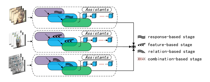
(a) Staged Knowledge Distillation (SKD).

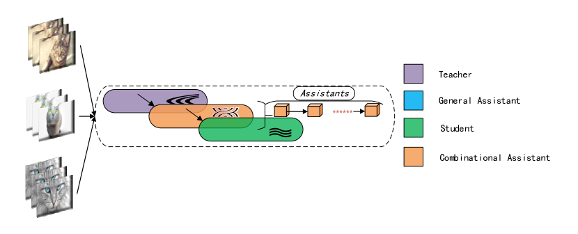
(b) Relevant Staged Knowledge Distillation (RSKD).

Figure 1: Architecture diagram of our proposed method. (a) SKD strategy. (b) RSKD strategy. The purple, blue, orange and green colors denote the teacher, general teaching assistant, combined teaching assistant and student, respectively. The shape of the line denotes the type of substage.

The field of KD has seen significant progress in recent years, with research focusing on the types of KD, loss functions, and the design of teacher-student architectures [34]. Different types of KD, including response-based [34], feature-based [31, 32, 35], and relation-based [33, 36], have been proposed to transfer knowledge from the teacher to the student. Researchers have also proposed various loss functions to enhance the student's performance, such as distilling knowledge with dense representations [37], attention-based knowledge distillation [38], and temperature-damping normalization [39]. Furthermore, different teacher-student architectures have been designed, including multiple teachers-students [40, 41, 42, 43, 44, 45, 46], self-training [47, 48], and mutual learning [49]. However, despite the abundance of research on the topic, there has been little attention paid to the internal relationship between the type of distillation method and the structural design of the teacher-student architecture.

KD is a process that mimics human learning by systematically transferring knowledge from a teacher model to a student model. To maximize the effectiveness of this process, we propose a novel framework called Staged Knowledge Distillation (SKD), which consists of three distinct learning stages, as shown in Figure 1(a). We argue that a blind, single-stage approach may be inefficient and ineffective due to its increased cost and potential for bias.

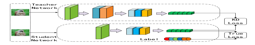
(a) Response-Based Substage.

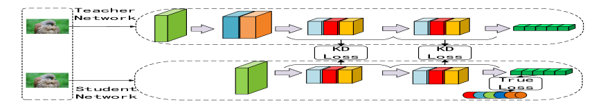
(b) Relation-Based Substage.

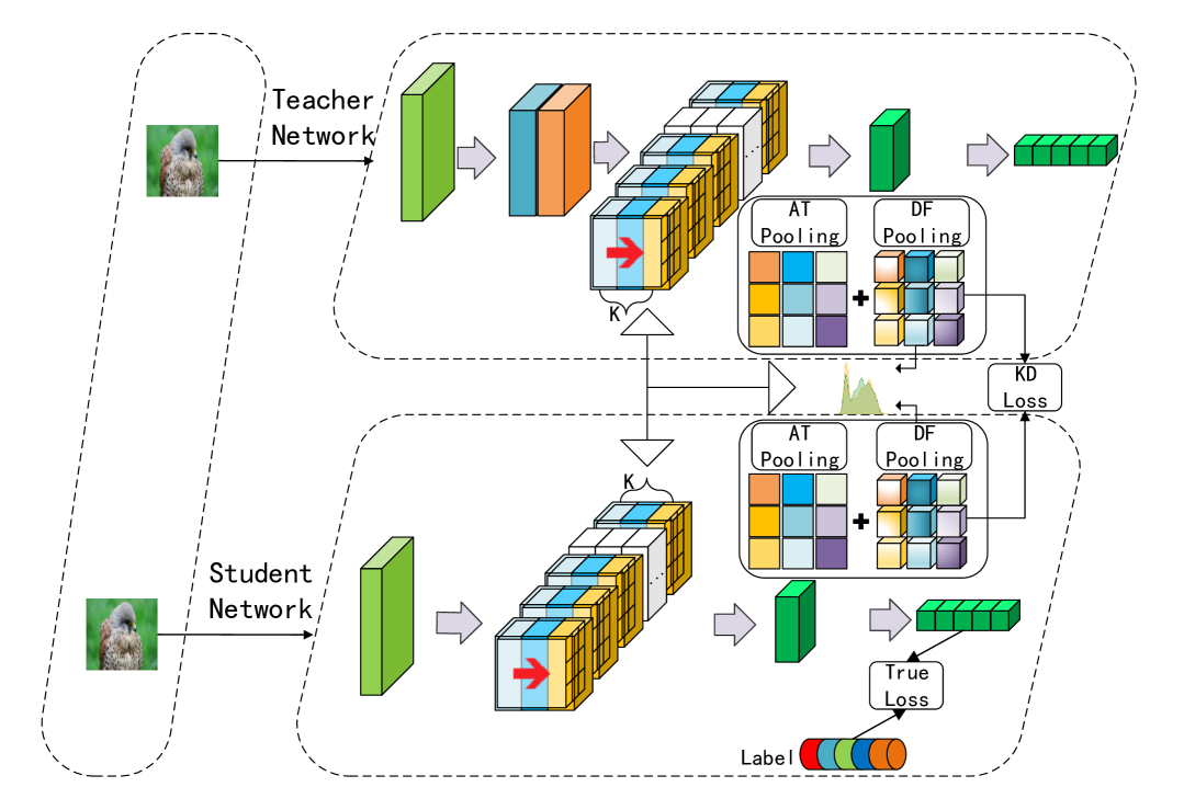
(c) Feature-Based Substage.

Figure 2: Illustration of three types of substages. (a) Response-Based Substage directly mimics the final result of the teacher model. (b) Relation-Based Substage explores the relationship between feature mapping pairs. (c) Feature-Based Substage focuses on the output distillation process of the intermediate feature layers.

To address this issue, we adopt a parallel multi-branch structure training method divided into three substages (see Figure 2), which emulates the human learning process and improves the algorithm's generalization ability. However, if the capacity gap between the teacher and the student is too large, the training effect will be diminished [46]. To overcome this limitation, we introduce the teaching assistant method [46], which we refer to as cascade training. Additionally, we use a weakly supervised label enhancement technique that generates high-quality pseudo labels to supervise the classification in the video.

The final student model in SKD is obtained by combining the results of each stage, which reduces the model's generalization error. However, the same learning framework is used internally for each parallel training branch, leading to the excessive correlation between models [50] and increased inference time and memory occupation when deployed. To address this issue, we propose a novel variant called Relevant Staged Knowledge Distillation (RSKD), which employs a combination stage (CS) approach, as illustrated in Figure 1(b). RSKD omits the ensemble process and instead uses a combination-based stage distillation.

Finally, we enhance the KD loss function between different processes to adapt to our proposed SKD and RSKD frameworks. For feature-based KD, we propose an improved method for comparing the distribution of feature dimensions (DF), which selects the teacher's top K channels and the student's K channels for distillation based on the original loss function. This improvement can significantly improve the effectiveness of distillation.

In this paper, we make several contributions to the field of knowledge distillation:

• We propose a new loss method, DF, which is based on the feature distribution and is able to uncover knowledge hidden in the distribution of features.

• We address traditional challenges in knowledge distillation by treating it as a stage learning problem and proposing a combination stage approach (CS).

• We propose two new weakly supervised distillation frameworks. The first, SKD, is a substage-integrated framework that simulates the human-stage learning process. The second, RSKD, is based on a relevant combination stage approach that improves efficiency and accuracy.

• We conducted extensive experiments on two analog data sets (CIFAR-100 and ImageNet) and one real data set (UCF101) [51], and demonstrate that our models achieve state-of-the-art and competitive results in video classification using knowledge distillation.

These contributions demonstrate the effectiveness of our proposed methods and provide insights into the potential of knowledge distillation for improving video classification models.

II Related Works

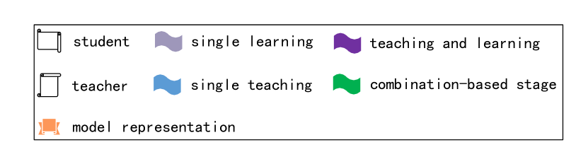
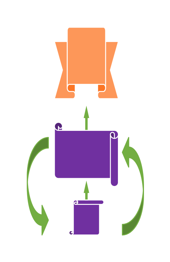
(a) ST.[47]

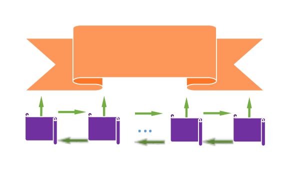
(b) ML.[49]

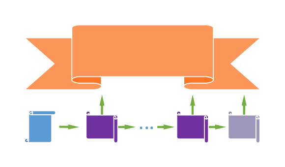
(c) OTM.[43]

(d) MTO.[44][42][41][40]

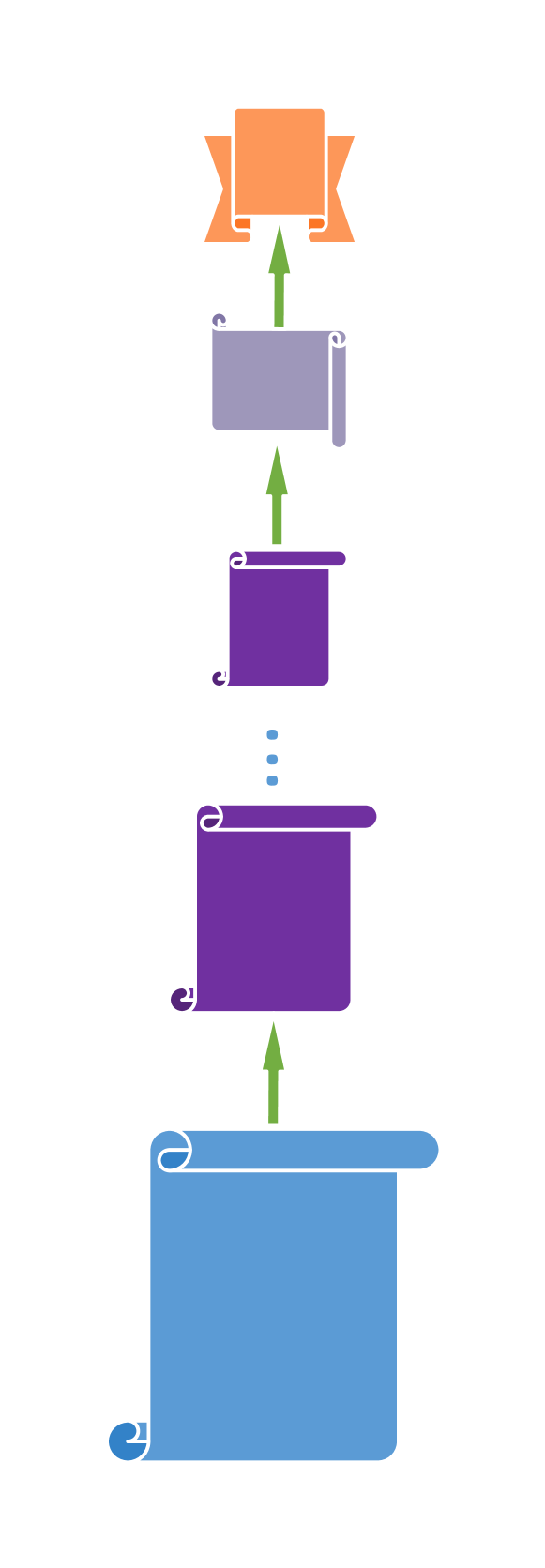
(e) AT.[46]

Figure 3: Five categories of teacher-student network design. The orientation represents model type: teacher or student; The color indicates function: teach or learn; The figure size represents model size; The final model is in orange.

II-A Weakly-Supervised Paradigms

Automatic video detection has gained increasing attention due to its usefulness in various intelligent surveillance systems. In recent years, research has focused on the weakly supervised learning paradigms due to the scarcity of clip-level annotations in video datasets [52, 53, 54, 55, 56].

Existing one-stage methods [54, 55, 56] rely on Multiple Instance Learning to describe anomaly detection as a regression problem and adopt an ordering loss approach. However, the lack of clip-level annotations often results in low accuracy. To address this issue, a two-stage approach based on self-training has been proposed [52, 53]. This approach generates pseudo-labels for clips and uses them to refine the discriminative representation. However, the generated pseudo-labels' uncertainty is not considered, which may negatively impact the classifier's performance.

II-B Types of Knowledge Distillation

Knowledge distillation (KD) was first proposed in [57] and has since been widely used to transfer knowledge from a large teacher network to a smaller student network [30]. Direct response-based distillation methods use softened label outputs to match the teacher and student predictions. However, they can be challenging to converge in some cases, leading to the development of feature-based distillation methods.

FitNets [31] proposed a two-stage method based on the middle layer to improve the performance of student networks. However, introducing an intermediate layer for dimension conversion may introduce additional parameters. Attention Transfer [32] introduced the attention mechanism to transform the feature information of each layer inside the teacher network to the student network.

Relation-based distillation explores the relationship between different layers in the teacher and student networks. In [33], the authors define the matrix correlation to measure the feature correlations between input and output layers of teachers and students. This method requires teachers and students to have the same structure, which limits the model's generalization ability.

II-C Structures of Knowledge Distillation

KD's teacher-student network structure design can be summarized into five categories, as shown in fig. 3.

The self-training method [47] belongs to fig. 3(a), where a poor teacher is used to train the student network. The teacher is trained to bypass the soft labels of the student through the label smoothing technique.

The authors of [49] propose a deep mutual learning strategy under fig. 3(b), in which a set of student networks learns and guides each other throughout the training process.

Instead of compressing the model, the student network [43] is trained with the same parameterization as the teacher network. The final result is obtained by combining the training results of multiple students and calculating their averages, falling under ensemble learning as shown in fig. 3(c).

As demonstrated in [42, 44], a model with multiple teachers and a single student is proposed to reduce the complexity of the student network. Subsequently, a novel collaborative teaching strategy [41] is proposed, leveraging the knowledge of two remarkable teachers to discover valuable information. Park [40] proposes a feature-based ensemble training method for KD, which employs multiple nonlinear transformations to transfer the knowledge of multiple teachers in parallel. These approaches can be visualized in fig. 3(d).

However, the primary issue with these approaches is that they rely on a single KD type, which can lead to a weakened distillation effect if there is a significant discrepancy between the teacher and student models. To address this, a novel distillation method for teaching assistants is proposed [46], as shown in fig. 3(e), which addresses the decreased KD efficiency when the gap between the teacher and student networks is too large. However, the lack of multi-type KD in stages results in a weak generalization ability of the model, making it challenging to apply to large-scale datasets and models.

III Proposed Method

In this section, we present our proposed method for knowledge distillation, which consists of three key components. First, we improve the loss function of the distillation substage to optimize the distillation process and make it adaptable to our proposed method. Second, we analyze the effectiveness of multi-branch stage distillation and propose a novel approach that combines distillation substages with less correlation within the structure to achieve maximum distillation effect. Finally, we introduce two new distillation methods, SKD and RSKD, which aim to simulate the learning process of the human stage as closely as possible by applying the substage and multi-branch combined distillation method. Together, our proposed method provides a comprehensive framework for efficient and effective knowledge distillation.

III-A Label Generation

To simulate a video classification dataset, we designed a composite-label generator inspired by the parallel multi-head classifier in [4]. The generator consists of an original-label generator and a pseudo-label generator. The main idea is to utilize a CycleGAN [58] to generate labels with relatively high approximate probabilities and then use random selection to generate labels with relatively low approximate probabilities (i.e., anomalous labels), and perform interpolation combinations.

As illustrated in fig. 4, the original-label image is generated by directly extracting the probability value from the corresponding position of the original image generated by the pre-training model. For the pseudo-label image, we utilized the pre-training module to process an input image obtained through random search and CycleGAN [58], and calculated the probability value of the corresponding position. The original-label image and the pseudo-label image are then combined to form a video package, which serves as the training set for the model.

Specifically, firstly, the forward network of the pre-training model calculates the probability values for each frame generated image to match the real labels. Then, using CycleGAN and random sampling techniques, each frame of static images is expanded into a package dataset, which is a combination of a sequence of continuous images, simulating a group of data frame images within a short time interval. Finally, the overall probability value of the package is obtained through weighted aggregation.

In general, when considering single-frame static images and simulated video package datasets, from the perspective of the loss function, the weighted processing of video frames does not fundamentally differ from the processing of individual frames. Therefore, it does not affect the accuracy of data processing.

(a) Original-label image.

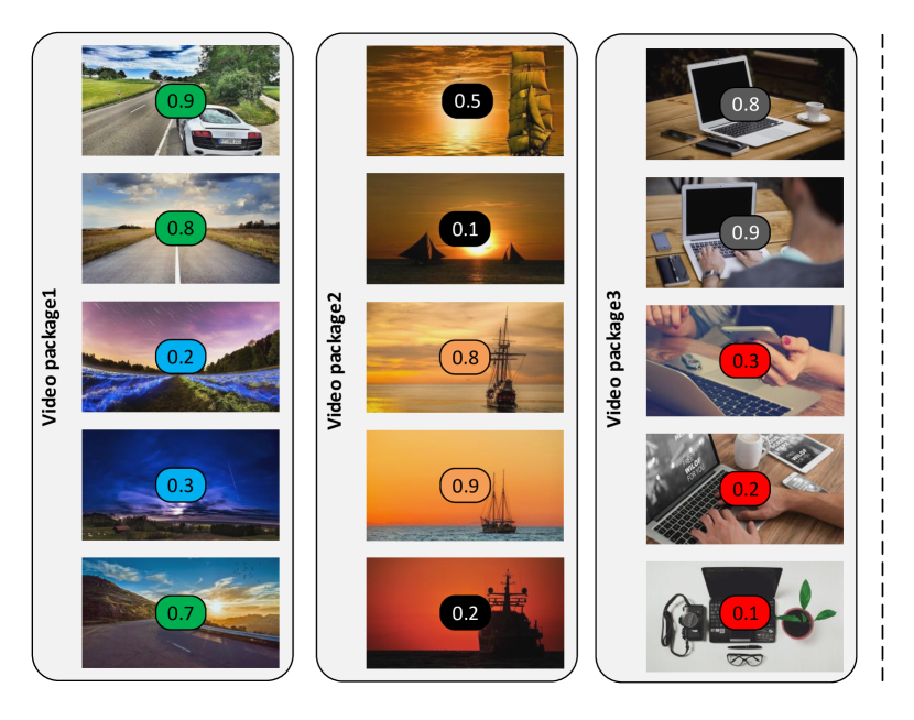
(b) Composite-label image.

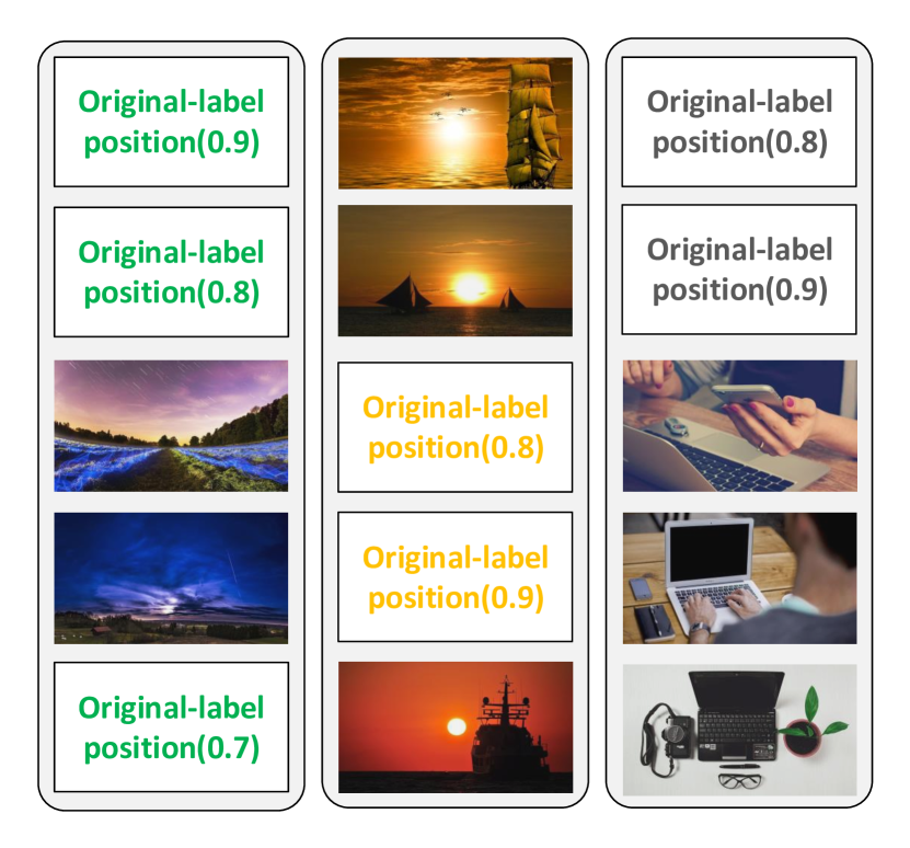
(c) Pseudo-label image.

Figure 4: The proposed process for generating pseudo-labels. The input image is fed into a pre-training model to obtain the original image label and its uncertainty. A reliable clip is selected based on this uncertainty, and pseudo-labels are generated for this clip using random search and the CycleGAN[58] method. The uncertainty of the pseudo-labels is calculated, and clip-level pseudo-labels are selected based on this uncertainty. The reliable and pseudo-labels are then combined to create a comprehensive video classification label package.

III-B Optimization of Substage KD

Response-based Substage

The response-based substage, depicted in fig. 2(a), can be formulated as follows:

$$\ell^{Rp}_{KD}(\vartheta^{Rp}_{T},\vartheta^{Rp}S)=\ell(\textRho_{S},{t})+\lambda\textKappa L(\boldsymbol{\varphi}(^{T})\parallel\boldsymbol{\varphi}(^{S})),$$ (1)

where $\ell(\cdot)$ is the cross-entropy loss between the student and the ground-truth labels, $\textKappa L(\cdot)$ is the KL divergence used to measure the consistency of the distribution between the teacher and the student, and $\lambda$ is a hyperparameter that balances the impact of KL divergence on the overall loss. ^T and ^S are the activation values of the teacher network as T and student network as S, $\textRho_{S}$ and ${t}$ are the direct output of S and the actual values of the labels, respectively.

The cross-entropy loss function $\ell(\textRho_{S},_{t})$ is computed as follows:

$$\ell(\textRho_{S},_{t})=\sum_{i=1}^{N}\textEta(\textRho_{S},_{t}),$$ (2)

where $\textEta(\cdot)$ denotes the cross-entropy loss function, and $N$ is the capacity of the training sample space. The probability of a student classification task can be defined as $\textRho_{S}=[r_{1},r_{2},\dots,r_{k},\dots,r_{C}]$, where $C$ denotes the number of classes. For each probability value $r_{k}$ in $\textRho_{S}$, it is computed using the softmax loss function:

$$r_{k}=\frac{exp(_{k})}{\sum^{C}_{j=1}exp({j})}.$$ (3)

In our case, KL divergence is used as the loss function for the classification task, which can be defined as follows:

$$\textKappa L=\sum^{C}_{i=1}\boldsymbol{\varphi}(y^{T}_{i})\cdot\log\left(\frac{\boldsymbol{\varphi}({y^{T}_{i}})}{\boldsymbol{\varphi}({y^{S}i})}\right),$$ (4)

where $y^{T}\in^{T}$, $y^{S}\in^{S}$, and $\boldsymbol{\varphi}(\cdot)$ denotes the probability distribution of activation values, which can be written as below:

$$\boldsymbol{\varphi}(\cdot)=\frac{\exp(\frac{y_{i}}{\textTau})}{\sum_{i=1}^{N}\exp(\frac{y_{i}}{\textTau})}$$ (5)

Here, $\textTau$ is a hyperparameter representing the distillation temperature.

Feature-based Substage

The feature-based substage, as illustrated in fig. 2(c), is a critical component of the knowledge distillation process, and it is formulated to ensure that the student network can mimic the teacher network's feature representation as accurately as possible. In this substage, the teacher-student feature mapping is accomplished by minimizing the loss function $\ell^{Fe}_{KD}(\vartheta^{Fe}_{T},\vartheta^{Fe}_{S})$, which is defined in eq. 1.

$$\begin{split}\!\ell^{Fe}_{KD}(\vartheta^{Fe}_{T},\vartheta^{Fe}_{S})=\ell(\textRho_{S},_{t})+\sum_{\begin{subarray}{c}i\in\varTheta\\ k\in S_{C}\end{subarray}}(\alpha\textMu(\!\digamma^{T}_{i},\!\digamma^{S}_{i})\\ +\beta\textMu\kappa(\!\digamma^{T}_{ik},\!\digamma^{S}_{ik})),\end{split}$$ (6)

where $\varTheta$ represents the number of layer pairs that need to be mapped and distilled between the teacher and student features, and $\textMu$ uses the attention transfer (AT)[32] loss function to train the feature vector of layers in the teacher-student network. The AT method accumulates the features across the channel dimensions to achieve dimensionality reduction, allowing teachers and students to maintain the same dimension when distilling features. However, this tends to lose the distribution of features on each channel. In many cases, the feature differences between channels not only exist in the global feature information but also are closely related to the feature distribution.

To address this issue, we propose the distribution of feature dimensions (DF) method, which compares the distribution of feature dimensions. Based on the need to ensure the similarity of the dimension distribution of the feature layer between teachers and students, this method combines the largest K channel values in the channel dimension and their corresponding location information to the pool. It maximizes the consistency of feature dimension distribution as much as possible. $\alpha$ and $\beta$ are two hyperparameters to balance the effect of AT versus DF in the overall loss. $\textMu(\digamma^{T}_{i},\digamma^{S}_{i})$ and $\textMu\kappa(\digamma^{T}_{ik},\digamma^{S}_{ik})$ are defined as follows:

$$\begin{split}\textMu(\digamma^{T}_{i},\digamma^{S}_{i})&=\parallel\frac{\digamma^{T}_{i}(\AA)}{\parallel\digamma^{T}_{i}(\AA)\parallel_{2}}-\frac{\digamma^{S}_{i}(\AA)}{\parallel\digamma^{S}_{i}(\AA)\parallel_{2}}\parallel_{2}\\ \textMu\kappa(\digamma^{T}_{ik},\digamma^{S}_{ik})&=\sum_{k\in S_{C}}\parallel\frac{\digamma^{T}_{ik}(\hat{P}\cdot\AA)}{\parallel\digamma^{T}_{ik}(\hat{P}\cdot\AA)\parallel_{2}}-\frac{\digamma^{S}_{ik}(\hat{P}\cdot\AA)}{\parallel\digamma^{S}_{ik}(\hat{P}\cdot\AA)\parallel_{2}}\parallel_{2},\end{split}$$ (7)

where $S_{C}$ denotes the collection of student channels in which we want to transfer feature maps.

$\digamma^{T}_{i}(\AA)=\sum^{Ch}_{j=1}\textAlpha_{j}^{2}$, where Ch is the number of channels in the ith layer, $\digamma$ is a feature mapping function, which can convert the 3D features of C×H×W into corresponding 2D features and $\textAlpha_{j}$ represents the 2D feature vector on the j channel. Unlike AT, DF considers the top K channels of the maximum feature dimension of the teacher, defined as $\digamma^{T}_{ik}(\hat{P}\cdot\AA)=\digamma^{T}_{i}(\hat{P_{k}}\cdot\textAlpha_{k}^{2})$, where $\hat{P_{k}}$ represents the position information vector corresponding to the feature of the k channel. This vector is used to determine the optimal channel selection for the teacher, allowing for the most efficient use of the available resources.

Relation-based Substage

In the relation-based substage, the goal is to measure the similarity between the internal structures of the teacher and student networks. To achieve this, we adopt the FSP matrix proposed by [33], which is a matrix that measures the inner product between two feature layers in the neural network. This matrix is computed using the weights of the feature layers of the teacher and student networks and can be formulated as follows:

$$\!\ell^{Re}_{KD}(\!\vartheta^{Re}_{T}\!,\!\vartheta^{Re}_{S})\!=\!\ell(\!\textRho_{S}\!,\!_{true})\!+\!\gamma\!\cdot\!\ell(\!G(W_{T})\!,\!G(W_{S})),$$ (8)

where $\textRho_{S}$ and _true denote the predicted and true labels of the student network, respectively. The FSP matrix $G(\cdot)$ is used to measure the similarity between the feature layers of the teacher and student networks. $\gamma$ is a hyperparameter that is used to balance the impact of FSP on the overall loss.

To compute the FSP matrix for the selected teacher-student, we denote $m$ as the selected input layer, $n$ as the selected output layer, $h$ as the height, and $w$ as the width. The FSP matrix can be computed as follows:

$$G_{(}m,n)(\cdot)=\sum_{i=1}^{h}\sum_{j=1}^{w}\frac{W_{(\cdot)m}\times W_{(\cdot)n}}{h\times w}.$$ (9)

Here, $W_{(\cdot)m}$ and $W_{(\cdot)n}$ are the weight matrices of the input and output layers of the selected teacher-student, respectively. The FSP matrix is normalized by the product of the height and width of the feature map to ensure that the values of the matrix are between 0 and 1. This normalization helps to reduce the impact of the size of the feature map on the FSP matrix.

The relation-based substage helps the student network to mimic the internal structure of the teacher network by measuring the similarity between their feature layers. The FSP matrix is a powerful tool for measuring this similarity and can help to improve the performance of the student network.

III-C Combination Stage

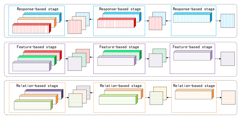
(a) SKD stage.

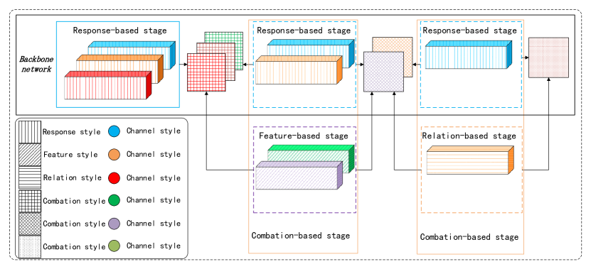
(b) RSKD stage.

Figure 5: Illustration of the processes of SKD and RSKD knowledge distillation, with divergent substage styles represented by distinct lines and assorted channel attribute styles by distinct hues. In SKD (a), the knowledge distillation process consists of three independent substages, while in RSKD (b), it includes the combination-based stage and the response-based KD substage implemented in the cascaded backbone network.

Algorithm 1 Transfer the distilled knowledge with SKD

0:    Teacher pre-training weight of each substage $\boldsymbol{\vartheta}^{Rp}_{\boldsymbol{T_{1}}}$, $\boldsymbol{\vartheta}^{Fe}_{\boldsymbol{T_{1}}}$, $\boldsymbol{\vartheta}^{Re}_{\boldsymbol{T_{1}}}$ Students randomly initialized weight of each substage $\boldsymbol{\vartheta}^{Rp}_{\boldsymbol{S_{1}}}$, $\boldsymbol{\vartheta}^{Fe}_{\boldsymbol{S_{1}}}$, $\boldsymbol{\vartheta}^{Re}_{\boldsymbol{S_{1}}}$ Number of cascading layers N

0:    Student training weight $\boldsymbol{\vartheta}^{Integration}_{\boldsymbol{S_{final}}}$ Stage 1: Initial stage distillation

1:  $\boldsymbol{\vartheta}^{Rp}_{\boldsymbol{S_{1}}}$ = arg min($\ell^{Rp}_{KD}$($\boldsymbol{\vartheta}^{Rp}_{\boldsymbol{T_{1}}}$ , $\boldsymbol{\vartheta}^{Rp}_{\boldsymbol{S_{1}}}$))

2:  $\boldsymbol{\vartheta}^{Fe}_{\boldsymbol{S_{1}}}$ = arg min($\ell^{Fe}_{KD}$($\boldsymbol{\vartheta}^{Fe}_{\boldsymbol{T_{1}}}$ , $\boldsymbol{\vartheta}^{Fe}_{\boldsymbol{S_{1}}}$))

3:  $\boldsymbol{\vartheta}^{Re}_{\boldsymbol{S_{1}}}$ = arg min($\ell^{Re}_{KD}$($\boldsymbol{\vartheta}^{Re}_{\boldsymbol{T_{1}}}$ , $\boldsymbol{\vartheta}^{Re}_{\boldsymbol{S_{1}}}$)) Stage 2: Cascade stage distillation

4:  for $i=1;i\leq N;$ do

5:     $\boldsymbol{\vartheta}^{Rp}_{S_{i+1}}$ = arg min($\ell^{Rp}_{KD}$($\boldsymbol{\vartheta}^{Rp}_{\boldsymbol{S_{i}}}$ , $\boldsymbol{\vartheta}^{Rp}_{\boldsymbol{S_{i+1}}}$))

6:     $\boldsymbol{\vartheta}^{Fe}_{\boldsymbol{S_{i+1}}}$ = arg min($\ell^{Fe}_{KD}$($\boldsymbol{\vartheta}^{Fe}_{\boldsymbol{S_{i}}}$ , $\boldsymbol{\vartheta}^{Fe}_{\boldsymbol{S_{i+1}}}$))

7:     $\boldsymbol{\vartheta}^{Re}_{\boldsymbol{S_{i+1}}}$ = arg min($\ell^{Re}_{KD}$($\boldsymbol{\vartheta}^{Re}_{\boldsymbol{S_{i}}}$ , $\boldsymbol{\vartheta}^{Re}_{\boldsymbol{S_{i+1}}}$))

8:  end forStage 3: Integration stage

9:  $\boldsymbol{\vartheta}^{Integration}_{\boldsymbol{S_{final}}}$ = avg($\boldsymbol{\vartheta}^{Rp}_{\boldsymbol{S_{N+1}}}$,$\boldsymbol{\vartheta}^{Fe}_{\boldsymbol{S_{N+1}}}$,$\boldsymbol{\vartheta}^{Re}_{\boldsymbol{S_{N+1}}}$)

Algorithm 2 Transfer the distilled knowledge with RSKD

0:    Teacher pre-training weight of each substage $\boldsymbol{\vartheta}^{Rp}_{\boldsymbol{T_{1}}}$, $\boldsymbol{\vartheta}^{Fe}_{\boldsymbol{T_{1}}}$, $\boldsymbol{\vartheta}^{Re}_{\boldsymbol{T_{1}}}$ Students randomly initialized weight of each combination-stage $\boldsymbol{\vartheta}^{Rp-CS}_{\boldsymbol{S_{1}}}$, $\boldsymbol{\vartheta}^{Fe-CS}_{\boldsymbol{S_{1}}}$, $\boldsymbol{\vartheta}^{Re-CS}_{\boldsymbol{S_{1}}}$ Number of cascading layers N

0:    Student training weight $\boldsymbol{\vartheta}^{Total}_{\boldsymbol{S_{final}}}$ Stage 1: Initial stage distillation

1:  $\boldsymbol{\vartheta}^{Rp-CS}_{\boldsymbol{S_{1}}}$ = arg min($\ell^{Rp-CS}_{KD}$($\boldsymbol{\vartheta}^{Rp}_{\boldsymbol{T_{1}}}$ , $\boldsymbol{\vartheta}^{Rp-CS}_{\boldsymbol{S_{1}}}$))

2:  $\boldsymbol{\vartheta}^{Fe-CS}_{\boldsymbol{S_{1}}}$ = arg min($\ell^{Fe-CS}_{KD}$($\boldsymbol{\vartheta}^{Fe}_{\boldsymbol{T_{1}}}$ , $\boldsymbol{\vartheta}^{Fe-CS}_{\boldsymbol{S_{1}}}$))

3:  $\boldsymbol{\vartheta}^{Re-CS}_{\boldsymbol{S_{1}}}$ = arg min($\ell^{Re-CS}_{KD}$($\boldsymbol{\vartheta}^{Re}_{\boldsymbol{T_{1}}}$ , $\boldsymbol{\vartheta}^{Re-CS}_{\boldsymbol{S_{1}}}$)) Stage 2: Cascade stage distillation

4:  for $i=1;i\leq N;$ do

5:     $\boldsymbol{\vartheta}^{Rp-CS}_{S_{i+1}}$ = arg min($\ell^{Rp-CS}_{KD}$($\boldsymbol{\vartheta}^{Rp-CS}_{\boldsymbol{S_{i}}}$ , $\boldsymbol{\vartheta}^{Rp-CS}_{\boldsymbol{S_{i+1}}}$))

6:     $\boldsymbol{\vartheta}^{Fe-CS}_{\boldsymbol{S_{i+1}}}$ = arg min($\ell^{Fe-CS}_{KD}$($\boldsymbol{\vartheta}^{Fe-CS}_{\boldsymbol{S_{i}}}$ , $\boldsymbol{\vartheta}^{Fe-CS}_{\boldsymbol{S_{i+1}}}$))

7:     $\boldsymbol{\vartheta}^{Re-CS}_{\boldsymbol{S_{i+1}}}$ = arg min($\ell^{Re-CS}_{KD}$($\boldsymbol{\vartheta}^{Re-CS}_{\boldsymbol{S_{i}}}$ , $\boldsymbol{\vartheta}^{Re-CS}_{\boldsymbol{S_{i+1}}}$))

8:  end forStage 3: Total stage distillation

9:  $\boldsymbol{\vartheta}^{Total}_{\boldsymbol{S_{final}}}$ = avg($\boldsymbol{\vartheta}^{Rp-CS}_{S_{N+1}}$,$\boldsymbol{\vartheta}^{Fe-CS}_{\boldsymbol{S_{N+1}}}$,$\boldsymbol{\vartheta}^{Re-CS}_{\boldsymbol{S_{N+1}}}$)

In the proposed improved (CS) design method, as shown in fig. 5(b), auxiliary branch substages are added in parallel for distillation, with a response-based substage serving as the backbone. Different combination stages are then composed of substages from different branches. This method introduces diversity in the substages used for distillation, which helps students learn more diverse and essential knowledge from teachers, and thus improves overall accuracy.

Although the diversity introduced may not be as accurate as the corresponding substages based on the response, it indirectly facilitates the learning of deep semantic features of distillation. This approach changes the style of substages of branches and the style of channels simultaneously, which enhances the generalization ability of students. This is particularly useful when the same substage is used for each distillation branch, which results in high style similarity between adjacent substages within the same branch, hindering the learning process of adjacent substages and diminishing the generalization ability of students, as shown in fig. 5(a).

It is worth noting that the combination of CS branches and the backbone network structure significantly affects the final KD. As ensemble models have demonstrated, the diversity of classifiers plays an essential role in boosting performance [50]. Similarly, the diversity introduced in the substages used for distillation can significantly improve the performance of KD. The improved CS design method achieves this by introducing diversity in the substages used for distillation.

III-D SKD and RSKD

The proposed SKD framework is based on the observation that different stages of KD have a phased impact on the final learning process. The training process of SKD mainly consists of three stages: response-based, feature-based, and relation-based. Each stage has a distinct purpose, allowing for a more comprehensive learning experience.

The response-based stage distills the teacher-student final output result, which is similar to the final result in the human learning process. The feature-based stage distills the specific layers that the teacher-student selects to distill, making them as similar as possible, akin to the shorter cycle in the human learning process. Lastly, the relation-based stage distills the similarity between specific layers at different scales, replicating the phased outcomes learned in the long human learning cycle. This multi-stage approach enables the student to learn both high-level and low-level knowledge from the teacher network.

The SKD training process is outlined in Algorithm 1. By leveraging the distinct advantages of each stage, our SKD framework provides a comprehensive and effective learning experience. However, integrating the output results of the three stages would lead to memory consumption and delay in the deployment model.

To address this, the proposed RSKD method forgoes the idea of an ensemble and instead uses a combination stage structure to combine the output results of different branch stages in the distillation process. This approach improves the model's generalization performance and reduces memory consumption and inference delay, achieving a balance between precision and efficiency, making it more conducive to model deployment in small embedded devices. As shown in fig. 5(b), the RSKD knowledge distillation process consists of a combination stage where different types of substage designs are used for each branch, with the backbone network using a response-based substage. The cascaded backbone network uses the response-based KD substage, and other auxiliary branch substages are added in parallel for distillation. Algorithm 2 details the RSKD training process.

IV Experiments

IV-A Experimental Setup

Datasets

We perform experiments on two public image classification benchmarks: CIFAR-100 and ImageNet. To synthesize pseudo-labels for the video classification images, we follow the method shown in fig. 4, which allows us to leverage the rich information in videos to improve image classification performance. We also used a real video action recognition dataset: UCF101 [51].

CIFAR-100 is a widely used image classification dataset that contains 32x32 images of 100 categories. The dataset comprises 50,000 training images, with 500 images for each class, and 10,000 test images, with 100 images for each class.

ImageNet is a well-known large-scale image classification dataset that consists of 1.2 million training images from 1,000 classes and 50,000 validation images. Unlike CIFAR-100, ImageNet better represents the real-world diversity and complexity of images.

UCF101 is a widely-used dataset for video action recognition, comprising around 13,000 video clips sourced from YouTube. It encompasses 101 distinct action categories, with each video clip having an average duration of approximately 7 seconds and a fixed resolution of 320x240 pixels.

Network Structure

We evaluate our method on two types of network structures: homogeneous and heterogeneous. Homogeneous networks refer to the network structures of a teacher and student network with the same architecture, allowing us to measure the performance gain of distillation in a like-for-like scenario. We consider three architectures for homogeneous networks: ResNet [59], Wide ResNet [60], and VGG [61]. For heterogeneous networks, we test our method on networks with different architectures for the teacher and student networks, which allows us to evaluate the generalization ability of our method across architectures. We consider four architectures for heterogeneous networks: ResNet, Wide ResNet, ShuffleNet [62], and MobileNet [63].

Implementation Details

TABLE I: The weight factor $\beta$ for different networks.

	FITNET[31]	AT[32]	AB[38]	FSP[33]	CRD[64]	DKD[37]
$\beta$	100	1000	0	0	0.8	8

To verify our method, we compared our proposed SKD and RSKD with KD[30], FITNET[31], AT[32], AB[38], FSP[33], CRD[64] and DKD[37] methods. To ensure a fair comparison, we implemented the algorithms of other methods based on their papers and codes.

For CIFAR-100 datasets, we expanded the original 32x32 images to 40x40 by filling 4 pixels on each side. We used randomly cropped 32x32 pixel images for training and kept the original 32x32 images for testing. We used pre-trained teachers as the initial teacher network. To maintain consistency, we set the weight factor $\beta$ that balances the actual loss with the distillation loss to the optimal value specified in the original text if available. Otherwise, we used the value obtained by grid search. The weight factor $\beta$ of different networks is shown in table I.

For the distillation of AB[38] and FSP[33], we used a separate pre-training phase, so $\beta$ was set to 0. The $\alpha$ of DKD[37] network was set to 1. We set the temperature parameter T = 4 and $\alpha$ = 0.9 for KD following [30]. All methods in our experiment were evaluated using SGD. Our SKD and RSKD algorithms used three substage cascades per process by default, and we set $\lambda$ to 0.9, $\alpha$ to 200, $\beta$ to 300, and $\gamma$ to 0.9.

For CIFAR-100, the initial learning rate of each stage cascade was 0.01 for MobileNetV2[65], ShuffleNetV1[62], and ShuffleNetV2[66], and 0.05 for other models. The learning rate decayed by a factor of 0.1 every 30 epochs after the first 120 epochs until the last 150 epochs, and the batch size was set to 128.

For ImageNet, we followed the standard PyTorch[67] practice, with each stage cascade having an initial learning rate of 0.2, a weight decay of 0.001 using the MSRA initialization technique[68], and a batch size of 256.

For UCF101, the pretrained model was trained from scratch using randomly initialized weights. Initially, it was trained for 200 epochs using SGD with a learning rate of 0.01 and weight decay of 0.0001. Subsequently, it was trained for an additional 100 epochs using Adam optimizer with a learning rate of 0.0002 and weight decay of 0.05. The batch size was set to 16 clips per GPU.

All training and validation processes were implemented using the PyTorch framework on an NVIDIA Tesla P100 industrial GPU server.

IV-B Details about RSKD

Formulation

The final distillation result of our formalized RSKD is given as follows:

$$\!\ell^{final}_{KD}\!=\!\ell(\textRho_{S},_{t})\!+\!\eta\cdot\!\ell^{Rp-CS}_{KD}+\!\xi\cdot\!\ell^{Fe-CS}_{KD}\!+\!\tau\cdot\!\ell^{Re-CS}_{KD},$$ (10)

where $\ell(\textRho_{S},_{t})$ represents the standard knowledge distillation loss, and $\eta$, $\xi$, and $\tau$ are hyperparameters that control the importance of the consistency losses. The ^Rp-CS, ^Fe-CS, and ^Re-CS superscripts refer to the response-based, feature-based, and response-feature-based consistency losses, respectively.

We believe that the effectiveness of RSKD for knowledge transfer may depend on the complexity of the datasets involved. Similar to the learning process of humans, when the knowledge to be mastered is elementary, the learning process is short and resembles the response-based substage. On the other hand, when the knowledge to be learned is complex, the learning process is long and resembles the feature-based and response-based substages. Therefore, inappropriate ratios of $\eta$, $\xi$, and $\tau$ may compromise the accuracy of the student model's predictions.

IV-C Comparison of Training Accuracy

Video Classification on CIFAR-100

The verification accuracy of top-1 is shown in table II and table III, where we evaluate RSKD on CIFAR-100. In the absence of an ensemble, table II presents the experimental results of teacher-student networks with the same network structure style, while table III shows the results of teacher-student networks with different network structure styles.

It is worth noting that while RSKD does not always achieve the optimal value in some teacher-student combinations when the teacher and student network styles are the same, it outperforms other distillation methods in experiments of different network architectures. This phenomenon can be explained by the fact that the small size of CIFAR-100 data may not fully demonstrate the advantages of stage learning in the same style of network architecture. Further discussion on this topic can be found in IV, V, IX, and VII.

The experimental results confirm that the CS structure in RSKD can uncover the hidden knowledge in different network architectures, leading to better distillation performance.

TABLE II: Results of student networks on CIFAR-100 (%), where teachers and students transfer across the same architectures. The table includes results obtained using a cascading strategy with three layers, denoted by $\ast$. The reported results are averaged over more than five runs.

Distillation Stage	Teacher Network	VGG13	WideResNet-40-2	ResNet56	ResNet32×4	ResNet110
	Student Network	VGG8	WideResNet-16-2	ResNet20	ResNet8×4	ResNet32
	Teacher	74.64	75.61	72.34	79.42	74.31
	Student	70.36	73.26	69.06	72.50	71.14
Response Stage	$\ast$KD[30]	73.98	75.92	71.26	73.69	73.58
	$\ast$AB[38]	71.54	72.90	69.71	73.52	71.26
	$\ast$DKD[37]	74.61	76.29	71.96	76.33	74.13
Feature Stage	$\ast$FITNET[31]	71.32	73.68	69.53	74.16	71.36
	AT[32]	71.63	74.31	70.65	73.97	72.54
	$\ast$CRD[64]	73.98	75.67	71.32	75.71	73.69
Relation Stage	$\ast$FSP[33]	70.63	73.10	70.04	72.82	71.95
Combination Stage	RSKD	74.59	76.32	71.82	76.53	74.21

TABLE III: Results of student networks on CIFAR-100 (%), where teachers and students transfer across different architectures. The table includes results obtained using a cascading strategy with three layers, denoted by $\ast$. The $\dagger$ symbol denotes the removal of the relation-based stage. The reported results are averaged over more than five runs.

Distillation Stage	Teacher Network	ResNet50	ResNet32×4	ResNet32×4	WideResNet-40-2
	Student Network	MobileNetV2	ShuffleNetV1	ShuffleNetV2	ShuffleNetV1
	Teacher	79.34	79.42	79.42	75.61
	Student	64.60	70.50	71.82	70.50
Response Stage	$\ast$KD[30]	68.51	75.11	75.35	75.94
	$\ast$AB[38]	67.76	73.79	74.83	73.69
	$\ast$DKD[37]	70.37	76.48	77.09	76.72
Feature Stage	$\ast$FITNET[31]	63.19	73.70	73.61	73.91
	AT[32]	59.02	71.92	72.91	73.46
	$\ast$CRD[64]	69.32	75.27	75.76	76.25
Combination Stage	RSKD$\dagger$	70.55	76.57	77.11	76.85

Video Classification on ImageNet

We evaluate our SKD, RSKD, and $\bullet$RSKD on ImageNet, and present the verification accuracy of top-1 and top-5 in table IV and table V, respectively. table IV contains the results of teachers and students having the same network architecture, while table V shows the results for teachers and students from different network architectures. To ensure experimental fairness, we employ ensemble and cascading strategies in all baseline models. Specifically, we use a three-level cascading and three-branch ensemble configuration as the default setting, allowing for a more accurate performance comparison.

The experimental results confirm our theoretical hypothesis that our SKD, RSKD, and $\bullet$RSKD achieve significant improvements on ImageNet with the increase of the data set. RSKD improves the accuracy of top-1 and top-5 by about 1% when compared with networks with the same teacher-student network style, while $\bullet$RSKD improves the accuracy of top-1 and top-5 by about 1%-1.5%. For networks with different teacher-student network styles, RSKD improves the accuracy of top-1 and top-5 by about 1%-1.5%, while $\bullet$RSKD improves the accuracy of top-1 and top-5 by about 1.5%-2%. Our methods outperform the most state-of-the-art distillation methods on ImageNet.

Video Classification on UCF101

We assessed the performance of our SKD, RSKD, and $\bullet$ RSKD techniques on the UCF101 dataset, and presented the validation accuracies for top-1 and top-5 in IX and VII respectively. IX encompasses the outcomes for both teachers and students with identical network architectures, while VII showcases the results obtained from teachers and students with distinct network architectures. To ensure the fairness of our experiments, we employed ensemble and cascading strategies across all baseline models. Specifically, we employed a default setup of a three-stage cascading and three-branch ensemble configuration, allowing for more precise performance comparisons.

The experimental results confirm our theoretical hypothesis that with the increase of real video data, our SKD, RSKD, and $\bullet$ RSKD techniques achieve significant improvements on UCF101. In comparison to networks with the same teacher-student network architecture, RSKD enhances the top-1 and top-5 accuracy by approximately 2%, while $\bullet$ RSKD achieves an improvement of about 2% - 3% in both top-1 and top-5 accuracy. For networks with different teacher-student network architectures, RSKD improves the top-1 and top-5 accuracy by approximately 2% - 2.5%, whereas $\bullet$ RSKD yields an enhancement of around 4% - 5% in top-1 and top-5 accuracy.

TABLE IV: Top-1 and Top-5 accuracy (%) of the student network ResNet-18 on ImageNet with teacher and student transfer across the same architectures. ResNet-34 is used as the teacher network and ResNet-18 as the student network. The $\bullet$ symbol indicates the ensemble strategy using three branches, and the $\ast$ symbol indicates the cascading strategy using three layers. The $\Uparrow$ symbol represents a performance improvement over classical KD. The results are averaged over more than three runs.

Distillation Stage			Response Stage		Feature Stage		Single Parallel Stage	Combination Stage
Accuracy	Teacher	Student	$\ast$KD$\bullet$[30]	$\ast$DKD$\bullet$[37]	$\ast$AT$\bullet$[32]	$\ast$CRD$\bullet$[64]	SKD	RSKD	$\bullet$RSKD
top-1	73.31	69.75	71.62	71.86	71.50	71.83	72.01$\Uparrow$	72.65$\Uparrow$	72.93$\Uparrow$
top-5	91.42	89.07	90.33	90.42	90.40	90.25	90.56$\Uparrow$	91.20$\Uparrow$	91.32$\Uparrow$

TABLE V: Top-1 and Top-5 accuracy (%) of the student network MobileNet-V1 on ImageNet with teacher and student transfer across different architectures. ResNet-50 is used as the teacher network and MobileNet-V1 as the student network. The $\bullet$ symbol indicates the ensemble strategy using three branches, and the $\ast$ symbol indicates the cascading strategy using three layers. The $\Uparrow$ symbol represents a performance improvement over classical KD. The results are averaged over more than three runs.

Distillation Stage			Response Stage		Feature Stage		Single Parallel Stage	Combination Stage
Accuracy	Teacher	Student	$\ast$KD$\bullet$[30]	$\ast$DKD$\bullet$[37]	$\ast$AT$\bullet$[32]	$\ast$CRD$\bullet$[64]	SKD	RSKD	$\bullet$RSKD$\dagger$
top-1	76.16	68.87	68.98	72.75	70.16	71.97	72.91$\Uparrow$	73.86$\Uparrow$	74.30$\Uparrow$
top-5	92.86	88.76	89.12	91.65	90.63	91.20	91.86$\Uparrow$	92.57$\Uparrow$	92.94$\Uparrow$

TABLE VI: Top-1 and Top-5 accuracy (%) of the student network ResNet-18 on UCF101 with teacher and student transfer across the same architectures. ResNet-34 is used as the teacher network and ResNet-18 as the student network. The $\bullet$ symbol indicates the ensemble strategy using three branches, and the $\ast$ symbol indicates the cascading strategy using three layers. The $\Uparrow$ symbol represents a performance improvement over classical KD. The results are averaged over more than three runs.

Distillation Stage			Response Stage		Feature Stage		Single Parallel Stage	Combination Stage
Accuracy	Teacher	Student	$\ast$KD$\bullet$[30]	$\ast$DKD$\bullet$[37]	$\ast$AT$\bullet$[32]	$\ast$CRD$\bullet$[64]	SKD	RSKD	$\bullet$RSKD
top-1	38.67	32.57	34.12	35.70	34.65	34.37	35.86$\Uparrow$	36.48$\Uparrow$	36.71$\Uparrow$
top-5	72.30	61.48	65.63	67.19	66.35	66.72	66.87$\Uparrow$	68.45$\Uparrow$	68.91$\Uparrow$

TABLE VII: Top-1 and Top-5 accuracy (%) of the student network MobileNet-V1 on UCF101 with teacher and student transfer across different architectures. ResNet-50 is used as the teacher network and MobileNet-V1 as the student network. The $\bullet$ symbol indicates the ensemble strategy using three branches, and the $\ast$ symbol indicates the cascading strategy using three layers. The $\Uparrow$ symbol represents a performance improvement over classical KD. The results are averaged over more than three runs.

Distillation Stage			Response Stage		Feature Stage		Single Parallel Stage	Combination Stage
Accuracy	Teacher	Student	$\ast$KD$\bullet$[30]	$\ast$DKD$\bullet$[37]	$\ast$AT$\bullet$[32]	$\ast$CRD$\bullet$[64]	SKD	RSKD	$\bullet$RSKD$\dagger$
top-1	40.62	36.71	37.54	38.26	37.60	37.92	38.52$\Uparrow$	39.17$\Uparrow$	40.06$\Uparrow$
top-5	76.61	65.18	67.94	70.25	68.46	69.11	70.39$\Uparrow$	72.06$\Uparrow$	73.69$\Uparrow$

IV-D Comparison of Training Efficiency

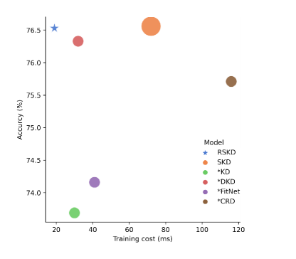
Figure 6: Comparison of accuracy and training time per batch on the CIFAR-100 dataset. The student network is ResNet8$\times$4 and the teacher network is ResNet32$\times$4.

TABLE VIII: Results of student networks on CIFAR-100, where teachers and students transfer across different architectures. The table includes results obtained using a cascading strategy with three layers, denoted by $\ast$.

	Top-1	Time	Params
$\ast$KD[30]	73.69	30	0
$\ast$DKD[37]	76.33	32	0
$\ast$FITNET[31]	74.16	41	46.5K
$\ast$CRD[64]	75.71	116	31.7M
SKD	76.56	72	62.3K
RSKD	76.53	19	42.3K

We evaluate the training costs of state-of-the-art distillation methods and demonstrate that RSKD is highly efficient. As illustrated in fig. 6 and table VIII, RSKD achieves an optimal balance between model performance and training costs. The training accuracy of RSKD surpasses the most advanced baseline distillation models while maintaining minimal training time and the same model size. Compared to SKD, RSKD is more efficient at only one-third of the size of SKD and saves nearly three times the training time.

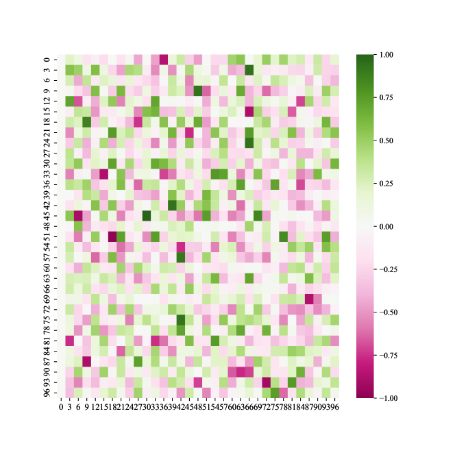
(a) SKD$\circ$.

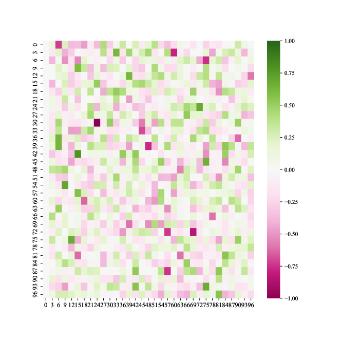
(b) SKD$\star$.

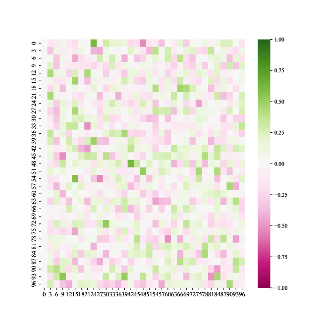
(c) SKD$\dagger$.

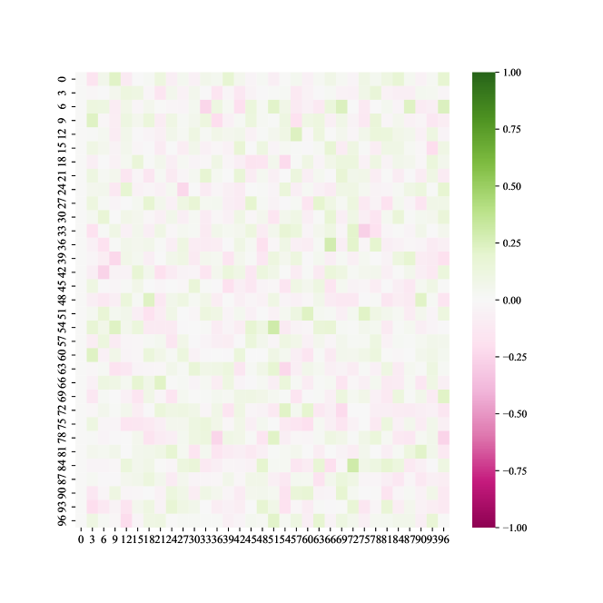
(d) RSKD.

Figure 7: Comparison of correlation matrices between teacher and student logits. We use ResNet56 as the teacher and ResNet20 as the student on CIFAR-100. The correlation matrices for different stages are shown: (a) Response-based stage ($\circ$), (b) Feature-based stage ($\star$), (c) Relation-based stage ($\dagger$), and (d) RSKD.

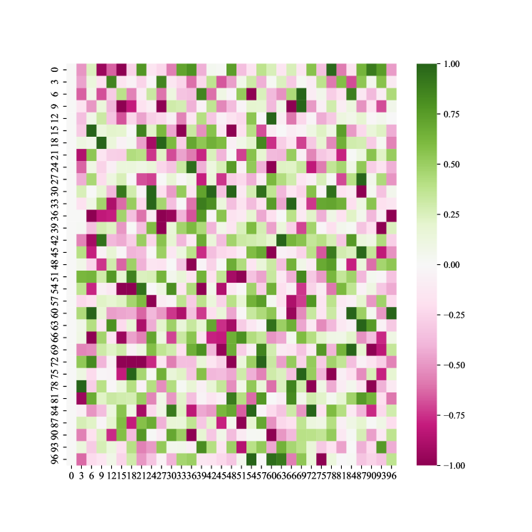
(a) SKD$\circ$

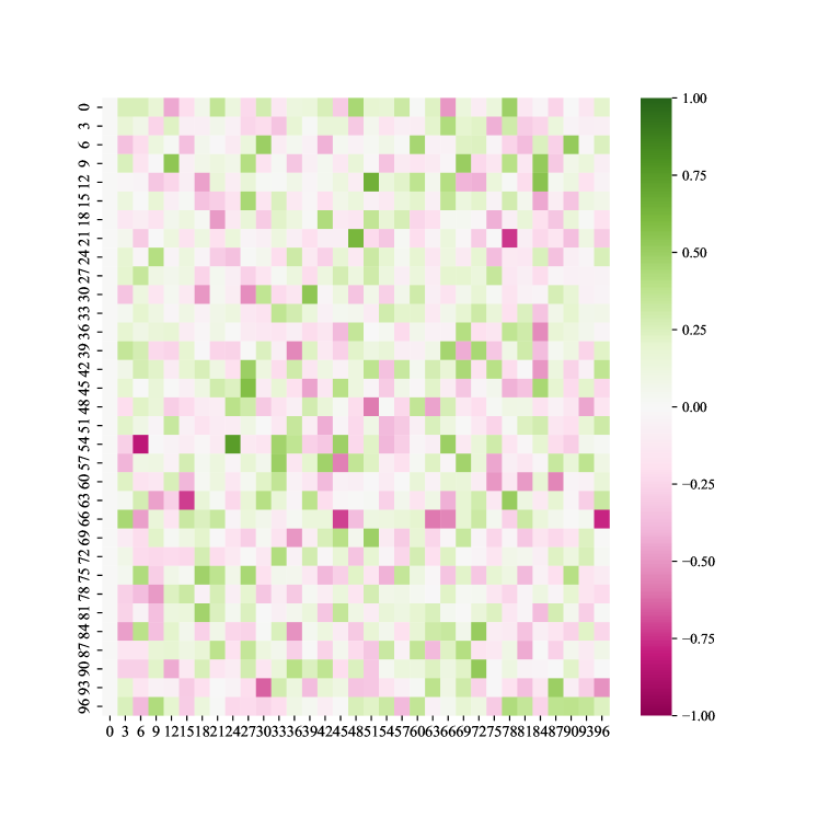
(b) SKD$\star$

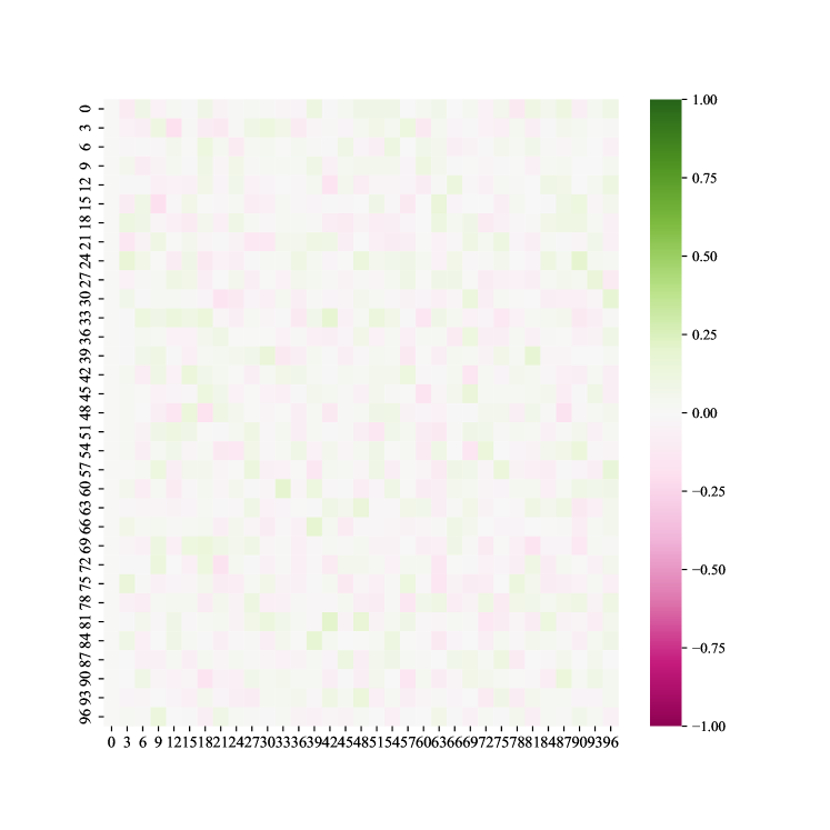
(c) RSKD$\dagger$

Figure 8: Differences in correlation matrices between teacher and student logits with the same network structure. (a) SKD$\circ$ indicates that the response-based stage is used only; (b) SKD$\star$ indicates that the feature-based stage is used only; (c) RSKD$\dagger$ with CS structure has the smallest difference, indicating a significant match between teachers and students compared to the above two methods. We set ResNet50 as the teacher and MobileNetV1 as the student on ImageNet. $\dagger$ indicates that the relation-based stage is removed.

IV-E Visualization of Correlation

We visualize the differences in correlation matrices between teacher and student logits for various distillation methods to demonstrate the effectiveness of RSKD in preserving the teacher's knowledge. In CIFAR-100, we compare four students: SKD$\circ$, SKD$\star$, SKD$\dagger$, and RSKD, as shown in fig. 7. The results indicate that RSKD achieves the most consistent correlation between teachers and students using the CS structure, resulting in highly similar logits with minimal discrepancies. This suggests that RSKD is a practical approach for preserving the teacher's knowledge in the student.

In ImageNet, we further evaluate the correlation between teacher and student logits for different combinations of teacher-student networks. fig. 8 demonstrate that RSKD minimizes the differences in correlation matrices for different teacher-student networks, indicating that RSKD can preserve the teacher's knowledge across different network architectures. Therefore, our method can generate student logits that closely resemble the teacher's, providing reliable results.

These results show that preserving the correlation between teacher and student logits is crucial for effective knowledge transfer in distillation. The preservation of correlation ensures that the student network reproduces the same predictions as the teacher network, even if the student network is smaller or has a different architecture than the teacher network. The correlation visualization provides further evidence that RSKD can effectively preserve the teacher's knowledge in the student network.

TABLE IX: Ablation study of RSKD on CIFAR-100, showing the impact of different components. The first column indicates whether cascading is used (\tiny{CA}⃝), while the second column indicates whether the Distilled Features (DF) method is employed (\tiny{DF}⃝). The following columns represent the effect of using different backbone networks for the correlation shaping (CS) module: \tiny{C-r}⃝ for the response-based backbone network, \tiny{C-f}⃝ for the feature-based backbone network, and \tiny{C-e}⃝ for the relation-based backbone network. The results are reported in terms of the top-1 accuracy (%) of the student network.

Teacher Student	Ablation					Top-1
	\scriptsize{CA}⃝	\scriptsize{DF}⃝	\scriptsize{C-r}⃝	\scriptsize{C-f}⃝	\scriptsize{C-e}⃝
ResNet56 ResNet20	-	-	-	-	-	69.82
	✓	-	-	-	-	71.76
	✓	✓	-	-	-	71.82
	✓	✓	✓	-	-	71.82
	✓	✓	-	✓	-	71.79
	✓	✓	-	-	✓	71.63
ResNet110 ResNet32	-	-	-	-	-	71.56
	✓	-	-	-	-	73.92
	✓	✓	-	-	-	74.06
	✓	✓	✓	-	-	74.21
	✓	✓	-	✓	-	74.11
	✓	✓	-	-	✓	74.07
ResNet32×4 ResNet8×4	-	-	-	-	-	73.67
	✓	-	-	-	-	75.89
	✓	✓	-	-	-	76.20
	✓	✓	✓	-	-	76.53
	✓	✓	-	✓	-	76.32
	✓	✓	-	-	✓	76.21
ResNet50 MobileNetV2	-	-	-	-	-	68.41
	✓	-	-	-	-	70.32
	✓	✓	-	-	-	70.39
	✓	✓	✓	-	-	70.55
	✓	✓	-	✓	-	70.43

TABLE X: Ablation study of RSKD on UCF101, showing the impact of different components. The first column indicates whether cascading is used (\tiny{CA}⃝), while the second column indicates whether the Distilled Features (DF) method is employed (\tiny{DF}⃝). The following columns represent the effect of using different backbone networks for the correlation shaping (CS) module: \tiny{C-r}⃝ for the response-based backbone network, \tiny{C-f}⃝ for the feature-based backbone network, and \tiny{C-e}⃝ for the relation-based backbone network. The results are reported in terms of the top-1 accuracy (%) of the student network.

Teacher Student	Ablation					Top-1
	\scriptsize{CA}⃝	\scriptsize{DF}⃝	\scriptsize{C-r}⃝	\scriptsize{C-f}⃝	\scriptsize{C-e}⃝
ResNet34 ResNet18	-	-	-	-	-	32.57
	✓	-	-	-	-	33.69
	✓	✓	-	-	-	34.12
	✓	✓	✓	-	-	36.48
	✓	✓	-	✓	-	36.10
	✓	✓	-	-	✓	35.64
ResNet50 MobileNetV1	-	-	-	-	-	36.71
	✓	-	-	-	-	37.24
	✓	✓	-	-	-	37.86
	✓	✓	✓	-	-	39.17
	✓	✓	-	✓	-	38.52

TABLE XI: Ablation study of DF in RSKD on ImageNet, showing the impact of different K values. The results are reported in terms of the top-1 accuracy (%) of the student network.

Teacher Student	Ablation							Top-1
	\scriptsize{CA}⃝	\scriptsize{C-r}⃝	2	4	8	16	32
ResNet34 ResNet18	✓	✓	✓	-	-	-	-	69.83
	✓	✓	-	✓	-	-	-	71.41
	✓	✓	-	-	✓	-	-	72.12
	✓	✓	-	-	-	\scriptsize{\checkmark}⃝	-	72.65
	✓	✓	-	-	-	-	✓	72.48
ResNet50 MobileNetV1	✓	✓	✓	-	-	-	-	72.68
	✓	✓	-	✓	-	-	-	73.43
	✓	✓	-	-	\scriptsize{\checkmark}⃝	-	-	73.86
	✓	✓	-	-	-	✓	-	73.57
	✓	✓	-	-	-	-	✓	73.21

IV-F Ablation Study

We conducted ablation experiments on the RSKD method to evaluate the impact of cascade operation, DF method, CS structure, and K value on the accuracy of CIFAR-100, ImageNet and UCF101 datasets. The results are presented in table IX, table X, and table XI.

Our experiments demonstrate that the response-based structure of the backbone network achieves optimal results in general. For small datasets with the same teacher-student model structure, the cascade operation and DF method have a more significant effect on the model performance. In contrast, reasonable CS structures have the same or slightly improved performance. However, the CS structure is more effective for models with larger datasets or different teacher-student model structures. This is because models with CS structures are less prone to overfitting, especially with a large amount of data or heterogeneous teacher-student networks.

The value of K is simultaneously determined using the grid search method. For teacher-student networks with the same structure, in the case of an optimal solution, the value of K tends to be larger. Conversely, for teacher-student networks with different structures, in the case of an optimal solution, the value of K is relatively smaller. This disparity arises from the fact that models with a homogeneous structure are more influenced by the first K channels in each layer, whereas heterogeneous models are less affected by the range of K values.

In summary, the RSKD method with the appropriate combination of cascade operation, DF method, and CS structure can significantly improve the model's accuracy, particularly for large or diverse datasets.

V Conclusion

In this paper, we have proposed novel weakly supervised teacher-student architectures, SKD and RSKD, that transform the KD process into a substage learning process, improving the quality of pseudo labels. We extensively investigate the relationship between the type of sub-stage learning process and the teacher-student structure, and demonstrate the validity of our method on the video classification task of CIFAR-100, ImageNet package dataset and UCF101 real dataset. Our analysis of the design methodology of the multi-branch substage composite structure and the optimization of the corresponding loss function has further validated the human-inspired design of the teacher-student network structure and substage learning process, leading to improved performance.

Importantly, our work is highly relevant to label-efficient learning on video data, which aims to explore new methods for video labeling and analysis. Our proposed SKD and RSKD methods offer promising approaches to improve the quality of pseudo labels in video classification tasks, which is a challenging problem due to the complexity and high dimensionality of video data. Inspired by human staged learning strategies, our approach offers an intuitive framework that is not limited to specific computer vision tasks. We believe that our strategies can be further applied to other computer video tasks such as video segmentation, single object tracking, and multiple object tracking. These tasks have gained considerable attention in the computer vision community, and we believe that our approach can be leveraged to enhance their performance as well. Overall, our work contributes to advancing the field of weakly supervised learning and can have significant practical implications in real-world applications.

Chao Wang received a B.E. degree in Process Equipment and Control Engineering from Jiangnan University in 2007, and an M.S. degree in Computer Application Technology from Northeast University in 2010. In the same year, he joined the China Academy of Railway Sciences and is currently an Assistant Researcher. Since assuming this position in 2012, he has been in charge of or involved in obtaining 8 invention patents and 3 utility model patents. His published papers cover interdisciplinary research topics in the fields of big data, neural networks, machine learning, and rail transportation. His research interests include intelligent rail transit systems, big data systems, cloud computing, computer vision, and graph neural networks related to machine learning. Chao Wang has led or participated in several key projects in China's rail transportation industry, achieving significant socioeconomic benefits. In 2021, his team won the second prize of the Science and Technology Progress of Beijing Rail Transit Society Award. The project he participated in received the first prize of the China Academy of Railway Sciences Award in 2020. In 2018, the project he led received the Innovation Award of the Communication Signal Research Institute. An invention patent he participated in won the China Excellent Patent Award in 2017.

Zheng Tang (M’16) earned his B.Sc. (Eng.) degree with Honors from the joint program by Beijing University of Posts and Telecommunications and Queen Mary University of London in 2014. He further obtained his M.S. and Ph.D. degrees in Electrical and Computer Engineering from the University of Washington in 2016 and 2019, respectively. In 2019, Dr. Tang joined Amazon as an Applied Scientist for the Amazon One team, serving there until 2021. Currently, he is a Senior Data Science Engineer at NVIDIA's Metropolis division, a position he has held since 2021. He has already had 3 U.S. patents and 17 peer-reviewed publications. His research interests include intelligent transportation systems, object tracking, re-identification, and other topics in the computer vision and machine learning realm. Dr. Tang has been an Associate Editor for the IEEE Transactions on Circuits and Systems for Video Technology since 2021, and an Organizing Committee Member for the AI City Challenge Workshops in conjunction with CVPR since 2020. He will also serve as the Challenge Chair for AVSS 2023, and previously served as an Area Chair for MLSP 2021. He received the Best AE Award of T-CSVT in 2021. A team he led triumphed in the 2nd AI City Challenge Workshop in CVPR 2018, securing the first rank in two tracks. Additionally, his paper was a finalist for two Best Student Paper Awards at ICPR 2016.

References

- [1] L. Yan, Q. Wang, S. Ma, J. Wang, and C. Yu, ``Solve the puzzle of instance segmentation in videos: A weakly supervised framework with spatio-temporal collaboration,'' IEEE Transactions on Circuits and Systems for Video Technology, 2022.
- [2] D. Liu, Y. Cui, L. Yan, C. Mousas, B. Yang, and Y. Chen, ``Densernet: Weakly supervised visual localization using multi-scale feature aggregation,'' ArXiv, vol. abs/2012.02366, 2020.
- [3] D. Liu, Y. Cui, L. Yan, C. Mousas, and Y. Chen, ``Densernet: Weakly supervised visual localization using multi-scale feature aggregation,'' 2020.
- [4] C. Zhang, G. Li, Y. Qi, S. Wang, L. Qing, Q. Huang, and M.-H. Yang, ``Exploiting completeness and uncertainty of pseudo labels for weakly supervised video anomaly detection,'' ArXiv, vol. abs/2212.04090, 2022.
- [5] C. Szegedy, W. Liu, Y. Jia, P. Sermanet, S. Reed, D. Anguelov, D. Erhan, V. Vanhoucke, and A. Rabinovich, ``Going deeper with convolutions,'' in Proceedings of the IEEE conference on computer vision and pattern recognition, 2015, pp. 1–9.
- [6] ChaoWang, ``Train intelligent testing system based on convolution neural network optimization algorithm,'' Railway Computer Application, vol. 28, no. 5, p. 6, 2019.
- [7] J. Ke, A. J. Watras, J.-J. Kim, H. Liu, H. Jiang, and Y. H. Hu, ``Towards real-time 3d visualization with multiview rgb camera array,'' Journal of Signal Processing Systems, vol. 94, pp. 329–343, 2022.
- [8] H. Mao, H. Liu, J. X. Dou, and P. V. Benos, ``Towards cross-modal causal structure and representation learning,'' in Machine Learning for Health, 2022.
- [9] W. Wang, T. Zhou, F. M. Porikli, D. J. Crandall, and L. V. Gool, ``A survey on deep learning technique for video segmentation,'' IEEE Transactions on Pattern Analysis and Machine Intelligence, vol. 45, pp. 7099–7122, 2021.
- [10] D. Wu, X. Dong, L. Shao, and J. Shen, ``Multi-level representation learning with semantic alignment for referring video object segmentation,'' 2022 IEEE/CVF Conference on Computer Vision and Pattern Recognition (CVPR), pp. 4986–4995, 2022.
- [11] C. Liang, W. Wang, T. Zhou, J. Miao, Y. Luo, and Y. Yang, ``Local-global context aware transformer for language-guided video segmentation,'' ArXiv, vol. abs/2203.09773, 2022.
- [12] D. Liu, Y. Cui, W. Tan, and Y. Chen, ``Sg-net: Spatial granularity network for one-stage video instance segmentation,'' 2021 IEEE/CVF Conference on Computer Vision and Pattern Recognition (CVPR), pp. 9811–9820, 2021.
- [13] Z. Qin, X. Lu, X. Nie, D. Liu, Y. Yin, and W. Wang, ``Coarse-to-fine video instance segmentation with factorized conditional appearance flows,'' IEEE/CAA Journal of Automatica Sinica, vol. 10, pp. 1192–1208, 2023.
- [14] W. Wang, J. Liang, and D. Liu, ``Learning equivariant segmentation with instance-unique querying,'' ArXiv, vol. abs/2210.00911, 2022.
- [15] X. Dong, J. Shen, F. M. Porikli, J. Luo, and L. Shao, ``Adaptive siamese tracking with a compact latent network,'' IEEE transactions on pattern analysis and machine intelligence, vol. PP, 2022.
- [16] J. Shen, Y. Liu, X. Dong, X. Lu, F. S. Khan, and S. C. H. Hoi, ``Distilled siamese networks for visual tracking,'' IEEE Transactions on Pattern Analysis and Machine Intelligence, vol. 44, pp. 8896–8909, 2019.
- [17] Z. Qin, S. Zhou, L. Wang, J. Duan, G. Hua, and W. Tang, ``Motiontrack: Learning robust short-term and long-term motions for multi-object tracking,'' ArXiv, vol. abs/2303.10404, 2023.
- [18] W. Wang, C. Han, T. Zhou, and D. Liu, ``Visual recognition with deep nearest centroids,'' ArXiv, vol. abs/2209.07383, 2022.
- [19] J. Liang, Y. Wang, Y. Chen, B. Yang, and D. Liu, ``A triangulation-based visual localization for field robots,'' IEEE CAA J. Autom. Sinica, vol. 9, pp. 1083–1086, 2022.
- [20] L. Yan, S. Ma, Q. Wang, Y. Chen, X. Zhang, A. E. Savakis, and D. Liu, ``Video captioning using global-local representation,'' IEEE Transactions on Circuits and Systems for Video Technology, vol. 32, pp. 6642–6656, 2022.
- [21] L. Yan, Q. Wang, Y. Cui, F. Feng, X. Quan, X. Zhang, and D. Liu, ``Gl-rg: Global-local representation granularity for video captioning,'' in International Joint Conference on Artificial Intelligence, 2022.
- [22] Z. Tang, G. Wang, H. Xiao, A. Zheng, and J.-N. Hwang, ``Single-camera and inter-camera vehicle tracking and 3d speed estimation based on fusion of visual and semantic features,'' 2018 IEEE/CVF Conference on Computer Vision and Pattern Recognition Workshops (CVPRW), pp. 108–1087, 2018.
- [23] Z. Tang, M. R. Naphade, M.-Y. Liu, X. Yang, S. Birchfield, S. Wang, R. Kumar, D. Anastasiu, and J.-N. Hwang, ``Cityflow: A city-scale benchmark for multi-target multi-camera vehicle tracking and re-identification,'' 2019 IEEE/CVF Conference on Computer Vision and Pattern Recognition (CVPR), pp. 8789–8798, 2019.
- [24] Z. Tang, M. R. Naphade, S. Birchfield, J. Tremblay, W. Hodge, R. Kumar, S. Wang, and X. Yang, ``Pamtri: Pose-aware multi-task learning for vehicle re-identification using highly randomized synthetic data,'' 2019 IEEE/CVF International Conference on Computer Vision (ICCV), pp. 211–220, 2019.
- [25] W. Chao, Z. Deming, X. Wei, and S. Xin, ``Cbtc software intelligent test system technology based on big data computing model,'' Railway Computer Application, vol. 29(7), pp. 30–35, 2020.
- [26] X. Guo, D. Wan, D. Liu, C. Mousas, and Y. Chen, ``A virtual reality framework to measure psychological and physiological responses of the self-driving car passengers,'' 2022.
- [27] D. Liu, Y. Cui, X. Guo, W. Ding, B. Yang, and Y. Chen, ``Visual localization for autonomous driving: Mapping the accurate location in the city maze,'' 2020 25th International Conference on Pattern Recognition (ICPR), pp. 3170–3177, 2020.
- [28] Q. Wang, Y. Fang, A. Ravula, R. He, B. Shen, J. Wang, X. Quan, and D. Liu, ``Deep partial multiplex network embedding,'' Companion Proceedings of the Web Conference 2022, 2022.
- [29] Z. Cheng, H. Choi, J. Liang, S. Feng, G. Tao, D. Liu, M. Zuzak, and X. Zhang, ``Fusion is not enough: Single-modal attacks to compromise fusion models in autonomous driving,'' ArXiv, vol. abs/2304.14614, 2023.
- [30] G. Hinton, O. Vinyals, J. Dean et al., ``Distilling the knowledge in a neural network,'' arXiv preprint arXiv:1503.02531, vol. 2, no. 7, 2015.
- [31] A. Romero, N. Ballas, S. E. Kahou, A. Chassang, C. Gatta, and Y. Bengio, ``Fitnets: Hints for thin deep nets,'' arXiv preprint arXiv:1412.6550, 2014.
- [32] S. Zagoruyko and Komodakis, ``Paying more attention to attention: Improving the performance of convolutional neural networks via attention transfer,'' arXiv preprint arXiv:1612.03928, 2016.
- [33] J. Yim, D. Joo, J. Bae, and J. Kim, ``A gift from knowledge distillation: Fast optimization, network minimization and transfer learning,'' in Proceedings of the IEEE conference on computer vision and pattern recognition, 2017, pp. 4133–4141.
- [34] J. Gou, B. Yu, S. J. Maybank, and D. Tao, ``Knowledge distillation: A survey,'' International Journal of Computer Vision, vol. 129, no. 6, pp. 1789–1819, 2021.
- [35] J. Kim, S. Park, and N. Kwak, ``Paraphrasing complex network: Network compression via factor transfer,'' Advances in neural information processing systems, vol. 31, 2018.
- [36] L. A. Gatys, A. S. Ecker, and M. Bethge, ``A neural algorithm of artistic style,'' arXiv preprint arXiv:1508.06576, 2015.
- [37] B. Zhao, Q. Cui, R. Song, Y. Qiu, and J. Liang, ``Decoupled knowledge distillation,'' in Proceedings of the IEEE/CVF Conference on Computer Vision and Pattern Recognition, 2022, pp. 11 953–11 962.
- [38] B. Heo, M. Lee, S. Yun, and J. Y. Choi, ``Knowledge transfer via distillation of activation boundaries formed by hidden neurons,'' in Proceedings of the AAAI Conference on Artificial Intelligence, vol. 33, no. 01, 2019, pp. 3779–3787.
- [39] C. Yang, L. Xie, S. Qiao, and A. L. Yuille, ``Training deep neural networks in generations: A more tolerant teacher educates better students,'' in Proceedings of the AAAI Conference on Artificial Intelligence, vol. 33, no. 01, 2019, pp. 5628–5635.
- [40] S. Park and N. Kwak, ``Feed: Feature-level ensemble for knowledge distillation,'' arXiv preprint arXiv:1909.10754, 2019.
- [41] H. Zhao, X. Sun, J. Dong, C. Chen, and Z. Dong, ``Highlight every step: Knowledge distillation via collaborative teaching,'' IEEE Transactions on Cybernetics, 2020.
- [42] S. You, C. Xu, C. Xu, and D. Tao, ``Learning from multiple teacher networks,'' in Proceedings of the 23rd ACM SIGKDD International Conference on Knowledge Discovery and Data Mining, 2017, pp. 1285–1294.
- [43] T. Furlanello, Z. Lipton, M. Tschannen, L. Itti, and A. Anandkumar, ``Born again neural networks,'' in International Conference on Machine Learning. PMLR, 2018, pp. 1607–1616.
- [44] Z. Yang, L. Shou, M. Gong, W. Lin, and D. Jiang, ``Model compression with two-stage multi-teacher knowledge distillation for web question answering system,'' in Proceedings of the 13th International Conference on Web Search and Data Mining, 2020, pp. 690–698.
- [45] A. Wu, W.-S. Zheng, X. Guo, and J.-H. Lai, ``Distilled person re-identification: Towards a more scalable system,'' in Proceedings of the IEEE/CVF Conference on Computer Vision and Pattern Recognition, 2019, pp. 1187–1196.
- [46] S. I. Mirzadeh, M. Farajtabar, A. Li, N. Levine, A. Matsukawa, and H. Ghasemzadeh, ``Improved knowledge distillation via teacher assistant,'' in Proceedings of the AAAI conference on artificial intelligence, vol. 34, no. 04, 2020, pp. 5191–5198.
- [47] L. Yuan, F. E. Tay, G. Li, T. Wang, and J. Feng, ``Revisiting knowledge distillation via label smoothing regularization,'' in Proceedings of the IEEE/CVF Conference on Computer Vision and Pattern Recognition, 2020, pp. 3903–3911.
- [48] Q. Xie, M.-T. Luong, E. Hovy, and Q. V. Le, ``Self-training with noisy student improves imagenet classification,'' in Proceedings of the IEEE/CVF conference on computer vision and pattern recognition, 2020, pp. 10 687–10 698.
- [49] Y. Zhang, T. Xiang, T. M. Hospedales, and H. Lu, ``Deep mutual learning,'' computer vision and pattern recognition, 2017.
- [50] L. I. Kuncheva and C. J. Whitaker, ``Measures of diversity in classifier ensembles and their relationship with the ensemble accuracy,'' Machine learning, vol. 51, no. 2, pp. 181–207, 2003.
- [51] K. Soomro, A. R. Zamir, and M. Shah, ``Ucf101: A dataset of 101 human actions classes from videos in the wild,'' ArXiv, vol. abs/1212.0402, 2012.
- [52] J. C. Feng, F. T. Hong, and W. S. Zheng, ``Mist: Multiple instance self-training framework for video anomaly detection,'' 2021.
- [53] S. Li, F. Liu, and L. Jiao, ``Self-training multi-sequence learning with transformer for weakly supervised video anomaly detection,'' 2023.
- [54] Y. Tian, G. Pang, Y. Chen, R. Singh, J. W. Verjans, and G. Carneiro, ``Weakly-supervised video anomaly detection with robust temporal feature magnitude learning,'' 2021.
- [55] J. Zhang, L. Qing, and J. Miao, ``Temporal convolutional network with complementary inner bag loss for weakly supervised anomaly detection,'' in 2019 IEEE International Conference on Image Processing (ICIP), 2019.
- [56] Y. Zhu and S. Newsam, ``Motion-aware feature for improved video anomaly detection,'' 2019.
- [57] C. Bucilua, R. Caruana, and A. Niculescu-Mizil, ``Model compression, in proceedings of the 12 th acm sigkdd international conference on knowledge discovery and data mining,'' New York, NY, USA, vol. 3, 2006.
- [58] J.-Y. Zhu, T. Park, P. Isola, and A. A. Efros, ``Unpaired image-to-image translation using cycle-consistent adversarial networks,'' in Proceedings of the IEEE international conference on computer vision, 2017, pp. 2223–2232.
- [59] K. He, X. Zhang, S. Ren, and J. Sun, ``Deep residual learning for image recognition,'' in Proceedings of the IEEE conference on computer vision and pattern recognition, 2016, pp. 770–778.
- [60] S. Zagoruyko and N. Komodakis, ``Wide residual networks,'' arXiv preprint arXiv:1605.07146, 2016.
- [61] K. Simonyan and A. Zisserman, ``Very deep convolutional networks for large-scale image recognition,'' arXiv preprint arXiv:1409.1556, 2014.
- [62] X. Zhang, X. Zhou, M. Lin, and J. Sun, ``Shufflenet: An extremely efficient convolutional neural network for mobile devices,'' in Proceedings of the IEEE conference on computer vision and pattern recognition, 2018, pp. 6848–6856.
- [63] A. G. Howard, M. Zhu, B. Chen, D. Kalenichenko, W. Wang, T. Weyand, M. Andreetto, and H. Adam, ``Mobilenets: Efficient convolutional neural networks for mobile vision applications,'' arXiv preprint arXiv:1704.04861, 2017.
- [64] Y. Tian, D. Krishnan, and P. Isola, ``Contrastive representation distillation,'' in International Conference on Learning Representations, 2020.
- [65] M. Sandler, A. Howard, M. Zhu, A. Zhmoginov, and L.-C. Chen, ``Mobilenetv2: Inverted residuals and linear bottlenecks,'' in Proceedings of the IEEE conference on computer vision and pattern recognition, 2018, pp. 4510–4520.
- [66] N. Ma, X. Zhang, H.-T. Zheng, and J. Sun, ``Shufflenet v2: Practical guidelines for efficient cnn architecture design,'' in Proceedings of the European conference on computer vision (ECCV), 2018, pp. 116–131.
- [67] A. Paszke, S. Gross, S. Chintala, G. Chanan, E. Yang, Z. DeVito, Z. Lin, A. Desmaison, L. Antiga, and A. Lerer, ``Automatic differentiation in pytorch,'' 2017.
- [68] K. He, X. Zhang, S. Ren, and J. Sun, ``Delving deep into rectifiers: Surpassing human-level performance on imagenet classification,'' in Proceedings of the IEEE international conference on computer vision, 2015, pp. 1026–1034.