Matrix product state approximations to quantum states of low energy variance

Abstract

We show how to efficiently simulate pure quantum states in one dimensional systems that have both finite energy density and vanishingly small energy fluctuations. We do so by studying the performance of a tensor network algorithm that produces matrix product states whose energy variance decreases as the bond dimension increases. Our results imply that variances as small as $\propto 1/\log N$ can be achieved with polynomial bond dimension. With this, we prove that there exist states with a very narrow support in the bulk of the spectrum that still have moderate entanglement entropy, in contrast with typical eigenstates that display a volume law. Our main technical tool is the Berry-Esseen theorem for spin systems, a strengthening of the central limit theorem for the energy distribution of product states. We also give a simpler proof of that theorem, together with slight improvements in the error scaling, which should be of independent interest.

I Introduction

It is widely established that entanglement is one of the most important concepts in the study of quantum many-body systems. The main reason why is that the character of entanglement in a system can typically be connected to fundamental physical properties. For instance, an area law in the low-energy states is associated with absence of criticality, localized correlations, and tensor network approximations Verstraete et al. (2006); Eisert et al. (2010). On the other hand, a larger amount of entanglement in the ground state can be associated to the appearance of quantum phase transitions Vidal et al. (2003).

The entanglement properties in the bulk of the spectrum, beyond the low energy sector, are also of crucial importance. For instance, the energy eigenstates of finite energy density (with zero energy variance) most often have large amounts of entanglement, compatible with their local marginals resembling Gibbs states as per the Eigenstate Thermalization Hypothesis (ETH) Srednicki (1994); Deutsch (1991). In contrast, product states are also in the bulk of the spectrum, but their lack of entanglement comes hand in hand with a larger energy variance.

Eigenstates and product states are the two extreme situations of either no energy variance or no entanglement. However, is this a fundamental trade-off? Or, alternatively, are there states that have both low entanglement and small energy variance? Here, we study this intermediate regime by answering the following question: what is the entanglement generated when narrowing down the variance of an initial quantum state? We do this by rigorously analyzing the performance of a matrix product state algorithm inspired by that in Bañuls et al. (2020) that decreases the energy variance of any initial product state, while only increasing the bond dimension in a controlled manner. As a main result, we show that vanishingly small energy variances $\delta^{2}$, down to $\delta^{2}\propto 1/\log(N)$, can be achieved with polynomial bond dimension, or $\log N$ entanglement entropy, in many models of interest.

Our method for studying the energy distribution at the output of the algorithm is based on the Berry-Esseen theorem Berry (1941); Esseen (1942) for spin systems. This result quantifies how much the energy distribution of product states resembles a Gaussian. We give a short proof of it based on the cluster expansion result from Wild and Alhambra (2023), improving previous ones by a polylogarithmic factor Brandao and Cramer (2015). This renders the bound optimal, and should be of independent interest. In our proofs, we use that approximate Gaussianity to estimate the energy average and variance of the state after a filtering operator has been applied to it. This filter is designed to narrow down the energy fluctuations, while being expressible as a tensor network with a bond dimension that can be easily upper bounded.

An additional motivation for this scheme is that it is expected that, under the ETH, any state with a low enough energy variance will also locally resemble a Gibbs state Dymarsky and Liu (2019); Bañuls et al. (2020). This idea is the basis of heuristic quantum algorithms for measuring local thermal expectation values Lu et al. (2021); Schuckert et al. (2023), in a way that is potentially amenable to near term quantum simulators Daley et al. (2022). With our bounds on the bond dimension of the MPS scheme, we rigorously analyze the classical simulability of those algorithms. In that sense, we narrow down the situations in which such a scheme will be computing quantities beyond the reach of classical computers. In doing so, we also offer efficiency guarantees for related tensor network algorithms Çakan et al. (2021); Lu et al. (2021); Yang et al. (2022).

The article is arranged as follows. We introduce the setting in Sec. II, and analyze the energy distribution of product states in Sec. III. The energy filter is introduced in Sec. IV, and in Sec. V we upper bound its bond dimension. We specialize to ETH Hamiltonians in Sec. VI and conclude. The more technical proofs are placed in the appendices.

II Preliminaries

We focus on systems of $N$ particles described by a local Hamiltonian

$$H=\sum_{i=1}^{N}h_{i}=\sum_{j}E_{j}\outerproduct{E_{j}}{E_{j}},$$ (1)

where each of the Hamiltonian terms is such that $\norm{h_{i}}\leq 1$, and overlaps with a small $\mathcal{O}(1)$ number of other qubits. If the Hamiltonian is in 1D (which we assume in Sec. V), this refers to adjacent sites on the chain. The spectrum $\{E_{j}\}$ is thus confined to the range $[-N,N]$. The initial states that we consider are product among all particles

$$\ket{p}=\bigotimes_{i}\ket{p_{i}}=\sum_{E_{j}}b_{j}\ket{E_{j}},$$ (2)

so that $b_{j}$ are the coefficients of the wavefunction in the energy eigenbasis. Their average and variance are

$$E=\bra{p}H\ket{p}=\sum_{E_{j}}|b_{j}|^{2}E_{j},$$ (3)

$$\sigma^{2}=\bra{p}(H-E)^{2}\ket{p}=\sum_{E_{j}}|b_{j}|^{2}(E_{j}-E)^{2}.$$ (4)

A mild but important assumption throughout this work is the following.

Assumption 1.

The ratio $\frac{\sigma}{\sqrt{N}}\equiv s$ is $\Omega(1)$ for all $N$.

It can be easily shown that, for product states, $\sigma=\mathcal{O}\left(\sqrt{N}\right)$. Thus, we are only assuming that the variance scales as fast as possibly allowed, which is a generic property of product states. With it we rule out trivial situations in which e.g. $\ket{p}$ is already an eigenstate of the Hamiltonian. Our goal will be to reduce the energy variance of these product states by applying a filtering operator, while controlling the amount of entanglement generated in the filtering process.

III Gaussian energy distribution

Due to the lack of correlations among all the sites, the energy distribution of a product state shares features with the distribution of $N$ independent random variables. Along these lines, the central limit theorem Hartmann et al. (2004) and the Chernoff-Höffding bound Anshu (2016); Kuwahara (2016) have previously been shown.

Here, we focus on a closely related but stronger result: the Berry-Esseen theorem Berry (1941); Esseen (1942). Originally, this showed that the cumulative distribution function of $N$ random variables is close to that of a Gaussian with the same average and variance, up to an error $\mathcal{O}(N^{-1/2})$. To introduce it in our context, let us define the following.

Definition 1.

Consider the cumulative function

$$J(x):=\sum\limits_{E_{j}\leq x}{|b_{j}|^{2}},$$ (5)

and the corresponding Gaussian cumulative function

$$G(x):=\int\limits_{-\infty}^{x}{\frac{dt}{\sqrt{2\pi\sigma^{2}}}e^{-\frac{(t-E)^{2}}{2\sigma^{2}}}}.$$ (6)

The Berry-Esseen error $\zeta_{N}$ is

$$\sup_{x}{|J(x)-G(x)|}\equiv\zeta_{N}.$$ (7)

The generalization of this definition to arbitrary states, and in particular mixed ones, is straightforward. The scaling of the error $\zeta_{N}$ with $N$ quantifies how much does the energy distribution deviate from the normal distribution. Our first technical result is the following.

Lemma 1.

Let $\ket{p}$ be a product state obeying Assumption 1. Then,

$$\zeta_{N}=\mathcal{O}(N^{-1/2}).$$ (8)

The proof is shown in Appendix A. It follows straightforwardly from the original Esseen’s inequality, together with the cluster expansion results from Wild and Alhambra (2023). Notice that this Lemma holds for all Hamiltonians that are few-body local, even beyond 1D.

Lemma 1 can be seen as a qualitative strengthening of Hartmann et al. (2004), where it was shown that in 1D $\lim_{N\rightarrow\infty}\zeta_{N}=0$. It also gives a poly-logarithmic improvement on the best previous bound Brandao and Cramer (2015); Brandão et al. (2015) which showed that $\zeta_{N}=\mathcal{O}\left(\frac{\log^{2D}N}{\sqrt{N}}\right)$ in a $D$ dimensional lattice. That result, however, also holds for the more general class of states with exponential decay of correlations, for which we expect the logarithmic factor is necessary Tikhomirov (1981).

The scaling of Eq. (8) is tight up to constant factors. For a specific example matching the bound, consider $N$ independent random coin tosses with equal probability, so that the probability of $k$ tails is (see Fig. 1)

$$p_{k}=\frac{1}{2^{N}}\binom{N}{k}.$$ (9)

Let $N$ be odd. Then, for $\frac{1}{2}N\geq x\geq\frac{1}{2}(N-1)$,

$$|J(x)-G(x)| =\left|\frac{1}{2}-\int\limits_{-\infty}^{x}{\frac{dt}{\sqrt{2\pi\sigma^{2}}}e^{-\frac{(t-\frac{1}{2}N)^{2}}{2\sigma^{2}}}}\right|$$ (10)

$$=\left|\int\limits_{0}^{\frac{1}{2}N-x}{\frac{dt}{\sqrt{2\pi\sigma^{2}}}e^{-\frac{(t-\frac{1}{2}N)^{2}}{2\sigma^{2}}}}\right|$$

$$\geq\frac{1}{\sqrt{\pi}}\left(\frac{\sqrt{2}\left(\frac{1}{2}N-x\right)}{\sigma}-\frac{\left(\frac{1}{2}N-x\right)^{3}}{\sqrt{2}\sigma^{3}}\right).$$

Choosing e.g. $x=\frac{1}{2}(N-\frac{1}{2})$ means the lower bound is $\Omega(\sigma^{-1})=\Omega(N^{-1/2})$.

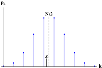
Figure 1: Representation of the binomial distribution $p_{k}$ in Eq. (9) for an odd value of $N$. For a non-interacting Hamiltonian with this distribution, the average energy is at $N/2$, where there is no eigenstate. The smallest standard deviation one can reach by filtering this distribution is limited to the difference between eigenergies at $k=\frac{N-1}{2}$ and $k=\frac{N+1}{2}$. We also illustrate a possible choice of $x$ in the derivation of Eq. (10).

Importantly, there are product states on spin systems with exactly Eq. (9) as the energy distribution. A trivial example is the state $\bigotimes_{i}^{N}\ket{+}_{i}$ with a non-interacting Hamiltonian $H=\sum_{i}\sigma_{Z,i}$. However, it also appears in certain Hamiltonians with strong interactions, such as the model considered in Schecter and Iadecola (2019), in which the product state has support on a $\mathcal{O}(N)$ number of eigenstates called quantum scars Turner et al. (2018); Alhambra et al. (2020).

IV Energy filter

We now define an operator which, when applied to any quantum state (in this case, our initial product state), will decrease its energy variance.

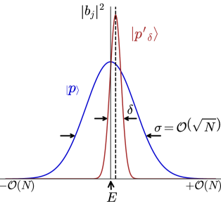
Figure 2: Illustration of the energy distribution of the initial product state, with standard deviation $\sigma$, and of the filtered distribution, with a smaller standard deviation $\delta$ and potentially a slightly shifted average (dashed line).

To do this, we first consider the cosine filter Ge et al. (2017); Bañuls et al. (2020)

$$P_{M}(E)=\cos^{M}\left(\frac{H-E}{N}\right).$$ (11)

For an ilustration of the effect of the filter on the energy distribution of the product state, see Fig. 2.

Since the eigenvalues of $\frac{H-E}{N}$ are within $[-1,1]$, the cosine function acts as an approximate projector around the energies close to $E$ when $M$ is very large. An advantage of this operator is that using the binomial expansion we can write

$$\cos^{M}\left(\frac{H-E}{N}\right)=\frac{1}{2^{M}}\sum\limits_{m=-\frac{M}{2}}^{\frac{M}{2}}c_{m}e^{i2m(H-E)/N}.$$ (12)

where $c_{m}=\binom{M}{\frac{M}{2}-m}$. There is some freedom as to how to define the denominator inside the cosine filter Yang et al. (2022), which does not change the final result significantly, so for simplicity we choose $N$ as in Eq. (11).

Eq. (12) shows that when the full operator $P_{M}(E)$ is applied to a trial state, the result can be written as a superposition of time evolution operators. Additionally, the amount of complex exponentials can be significantly reduced for a small cost in precision.

Lemma 2.

Let the approximate cosine function $g_{y}(x)$ be

$$g_{y}(x):=\frac{1}{2^{M}}\sum\limits_{m=-y\sqrt{M}}^{y\sqrt{M}}{\binom{M}{\frac{M}{2}-m}e^{i2mx}}.$$ (13)

This is such that, $\forall x\in[-1,1]$,

$$|\cos^{M}(x)-g_{y}(x)|\leq e^{-\frac{y^{2}}{2}}.$$ (14)

This is obtained from the Chernoff bound on the binomial coefficients, which is exponentially decaying in $y^{2}$. For a significant reduction in the number of terms, we need $y$ to be $o(\sqrt{M})$.

Lemma 2 allows us to define our filtered state as

$$\ket{p_{M,y}}=\frac{g_{y}\left(\frac{H-E}{N}\right)\ket{p}}{\norm{g_{y}\left(\frac{H-E}{N}\right)\ket{p}}},$$ (15)

which leads to the main technical result of this section.

Lemma 3.

Let $M=\mathcal{O}\left(\frac{N}{\zeta_{N}^{2}}\right)$ and $M=\Omega(N)$, and $y=\Omega\left(\sqrt{\log\left(M^{3}/N^{2}\right)}\right)$. The energy average $\mu$ and variance $\delta^{2}$ of $\ket{p_{M,y}}$ are bounded as

$$|\mu-E| =\mathcal{O}\left(\frac{N}{\sqrt{M}}\right),$$ (16)

$$\delta^{2} =\mathcal{O}\left(\frac{N^{2}}{M}\right).$$ (17)

This lemma only applies for large enough values of $M$. On the other hand, for $M=\mathcal{O}(N)$, the best bounds one can achieve are

$$|\mu-E| =\mathcal{O}\left(\sqrt{N}\right),$$ (18)

$$\delta^{2} =\mathcal{O}\left(N\right),$$ (19)

which means that the filter does not change the variance in a substantial way - at most up to a constant factor.

For large $M$, the lemma shows that the filter $g_{y}\left(\frac{H-E}{N}\right)$ decreases the energy variance of the state without changing the average energy too much. The proof is shown in App. B. It is based on the Berry-Esseen error from Definition 1, which we use to approximate the expression of the variance $\delta^{2}$ as a Gaussian integral, with a considerable amount of error terms that need to be estimated. We note that this holds for Hamiltonians that are local, independent of the dimension. The upper bound on $M$ in terms of $\zeta_{N}^{-1}$ is due to the fact that the deviation from Gaussian limits how much we can resolve the energy distribution after the filter is applied: if the deviation is large, the filter may act in a more uncontrolled way, and the bound may not hold.

In many practical scenarios we expect the wavefunction $\ket{p}$ to be symmetric about the energy average, in which case $\mu$ and $E$ will be identical. On the other hand, the scaling of the bound on $\delta$ is tight up to constant factors: if the wave-function coefficients $b_{j}$ are taken to be an exact Gaussian, one can explicitly calculate $\delta\simeq\frac{N}{\sqrt{2M}}$ (see Eq. (15) in Bañuls et al. (2020)).

The result is purposely stated in terms of the general error from Def. 1. Lemma 1, however, allows us to establish that choosing $M\propto N^{2}$, the bound on the variance is

$$\delta^{2}=\mathcal{O}(1).$$ (20)

This means that for any initial product state with standard deviation of $\mathcal{O}(\sqrt{N})$, the cosine filter can be applied to reduce the standard deviation down to $\mathcal{O}(1)$, and shifting the average by at most that amount. The examples from Sec. III show that this is the smallest variance one can reach in general (see Fig. 1). However, if the factor $\zeta_{N}$ would decrease more quickly than $\mathcal{O}(N^{-1/2})$, the range of values which $M$ can take becomes larger, and lower variances can be achieved, as we discuss in Sec. VI.

V Low variance state using MPS

In this section we prove our main result on the approximability of the filtered states with matrix product states. The main idea is that it is possible to construct a matrix product operator $g_{y}^{D}$ that approximates $g_{y}\left(\frac{H-E}{N}\right)$ in one spatial dimension. When applied to our initial product state $|p\rangle$, this implies that one can efficiently find an MPS approximation to $|p_{M,y}\rangle$ with a close enough average and variance in energy, while also having a small bond dimension. This is contained in our main result Theorem 1.

The starting point is the following lemma from Kuwahara et al. (2021), which shows there is a Matrix Product Operator (MPO) Pirvu et al. (2010) approximation to the matrix exponential of $H$ .

Lemma 4.

Kuwahara et al. (2021) Let $H$ be a 1D local Hamiltonian. There is an algorithm that outputs an MPO approximation $T_{t}$ of $e^{-itH}$ such that

$$\norm{T_{t}-e^{-itH}}\leq\epsilon,$$ (21)

with bond dimension upper bounded by

$$D\leq e^{\mathcal{O}(t)+\mathcal{O}\left(\sqrt{t\log(N/\epsilon)}\right)}.$$ (22)

The idea here is that $g_{y}$ can be written as a sum of complex exponentials as per Eq. (12). Thus, we can approximate each term in the filter with Lemma 4, and add them to obtain our approximate filter

$$g_{y}^{D}=\frac{1}{2^{M}}\sum\limits_{m=-y\sqrt{M}}^{m=+y\sqrt{M}}{\binom{M}{\frac{M}{2}-m}T_{2m/N}}.$$ (23)

When applied to the initial product state , this yields the final MPS with bounded variance and bond dimension. The precise result is as follows.

Theorem 1.

Let $H$ be one-dimensional, and let $\ket{p}$ satisfy Assumptions 1. The MPS $|p^{\prime}_{\delta}\rangle=\frac{g_{y}^{D}\ket{p}}{||g_{y}^{D}\ket{p}||}$, under the conditions of Lemma 3, has the properties

$$|\langle p^{\prime}_{\delta}|H|p^{\prime}_{\delta}\rangle-E| =\mathcal{O}\left(\frac{N}{\sqrt{M}}\right)$$ (24)

$$\langle p^{\prime}_{\delta}|H^{2}|p^{\prime}_{\delta}\rangle-\left(\langle p^{\prime}_{\delta}|H|p^{\prime}_{\delta}\rangle\right)^{2} \leq 2\delta^{2}=\mathcal{O}\left(\frac{N^{2}}{M}\right).$$ (25)

Moreover, the bond dimension of $g_{y}^{D}$ (and thus of $\ket{p^{\prime}_{\delta}}$) is bounded by

$$D\leq\frac{N\log N}{\delta}e^{\mathcal{O}\left(\frac{\sqrt{\log(N/\delta)}}{\delta}\right)+\mathcal{O}\left(\frac{\log^{\frac{3}{4}}(N/\delta)}{\sqrt{\delta}}\right)}.$$ (26)

Proof.

First we have that, by Lemma 4 and the triangle inequality,

$$\begin{split}\norm{g_{y}\left(\frac{H-E}{N}\right)-g_{y}^{D}}&\leq 2^{-M}\sum_{|m|\leq y\sqrt{M}}\binom{M}{\frac{M}{2}-m}\epsilon\\ &\leq\epsilon,\end{split}$$ (27)

where we consider the approximation error $\epsilon$ coming from Eq. (21). Thus, for the states

$$||\ket{p_{M,y}}-\ket{p^{\prime}_{\delta}}|| =||\frac{g_{y}\left(\frac{H-E}{N}\right)\ket{p}}{\norm{g_{y}\left(\frac{H-E}{N}\right)\ket{p}}}-\frac{g_{y}^{D}\ket{p}}{\norm{g_{y}^{D}\ket{p}}}||$$ (28)

$$\leq 2\frac{\norm{g_{y}\left(\frac{H-E}{N}\right)-g_{y}^{D}}}{\norm{g_{y}\left(\frac{H-E}{N}\right)\ket{p}}}$$ (29)

$$\leq\frac{2\ \epsilon}{\norm{g_{y}\left(\frac{H-E}{N}\right)\ket{p}}}.$$ (30)

The factor $\norm{g_{y}\left(\frac{H-E}{N}\right)\ket{p}}$ is lower bounded in Eq. (106) as,

$$\norm{g_{y}\left(\frac{H-E}{N}\right)\ket{p}}=\Omega\left(\frac{N^{1/2}}{M^{1/4}}\right).$$ (31)

Now, notice that for $\ket{p_{M,y}}$ and $\ket{p^{\prime}_{\delta}}$ to have the same average and variance up to the errors of Eq. (24) and (25) it is enough that,

$$||\ket{p_{M,y}}-\ket{p^{\prime}_{\delta}}||\leq\frac{\delta^{2}}{2N^{2}}.$$ (32)

Given Eq. (32), the error we require from Lemma 4 is $\epsilon=\mathcal{O}\left(\frac{\delta^{2}}{N^{3/2}M^{1/4}}\right)$. With this, notice that the leading error for the average is given by Eq. (16).

To estimate the total bond dimension of $g_{y}^{D}$, notice that we have $2y\sqrt{M}$ terms, and that, considering Lemma 3, the longest $t$ to consider is $y\sqrt{M}/N=\mathcal{O}(y\delta^{-1})$. Using Lemma 4 and simplifying the powers in the logarithm, we can upper bound

$$D\leq\frac{2yN}{\delta}e^{\mathcal{O}\left(y\delta^{-1}\right)+\mathcal{O}\left(\sqrt{y\delta^{-1}\log\left(\frac{N}{\delta}\right)}\right)}$$ (33)

Finally, choosing $y^{2}=6\log\frac{N}{\delta}$ as allowed by Lemma 3, we obtain

$$D\leq\frac{N\log N}{\delta}e^{\mathcal{O}\left(\frac{\sqrt{\log(N/\delta)}}{\delta}\right)+\mathcal{O}\left(\frac{\log^{\frac{3}{4}}(N/\delta)}{\sqrt{\delta}}\right)}.$$ (34)

∎

Additionally, the run-time of the algorithm that constructs $|p^{\prime}_{\delta}\rangle$ is simply the bond dimension multiplied by a factor of $N$, to account for the cost of manipulating the tensors of the MPO Kuwahara et al. (2021).

The most important particular case of this result is if we aim for a variance $\delta=\mathcal{O}(1)$, in which case we have the following.

Corollary 1.

There exists an MPS $\ket{p^{\prime}}$ of quasilinear bond dimension $D\leq Ne^{\mathcal{O}(\log^{\frac{3}{4}}(N))}$ such that

$$|\langle p^{\prime}|H|p^{\prime}\rangle-E| =\mathcal{O}(1)$$ (35)

$$\langle p^{\prime}|H^{2}|p^{\prime}\rangle-(\langle p^{\prime}|H|p^{\prime}\rangle)^{2} =\mathcal{O}(1).$$ (36)

This is achieved by choosing $M\propto N^{2}$ in the filter, given Theorem 1 together with Lemma 3. This is the smallest variance that can be achieved in general, as illustrated by the examples with the binomial energy distribution in Eq. 9.

If instead of a product state our initial state has exponential decay of correlations, the corresponding standard deviation one can prove to reach in general is $\delta=\mathcal{O}(\log^{2D}N)$ as per the result in Brandão et al. (2015). Additionally, if the Berry-Esseen error $\zeta_{N}$ is much smaller than the upper bound of Lemma 1 we can also reach smaller variances, down to $\zeta_{N}^{2}\times N$, at an additional cost in the bond dimension. In particular, we expect it is most often possible to reach $\delta^{2}\propto 1/\log{N}$ while still keeping the bond dimension from Eq. (26) polynomial in $N$.

Theorem 1 is restricted to one dimension. For higher dimensions, the existence of a similar PEPO is guaranteed by the results of Molnar et al. (2015), which in our setting yields a bond dimension

$$D=\left(\frac{N}{\delta}\right)^{O(\frac{\sqrt{\log N}}{\delta})}.$$ (37)

This, however, is only polynomial for larger variances $\delta^{2}=\Omega(\log N)$ and in no case guarantees a provably efficient approximation algorithm, considering the difficulty of contracting PEPS Schuch et al. (2007).

The upper bounds on the bond dimension also guarantee bounds on the entanglement entropy of the state $\ket{p^{\prime}_{\delta}}$. Defining $S(\rho^{\prime}_{A})=-\tr[\rho^{\prime}_{A}\log\rho^{\prime}_{A}]$ with $\rho^{\prime}_{A}$ the marginal on region $A$, we have that $S(\rho^{\prime}_{A})\leq|\partial_{A}|\log D$, with $|\partial_{A}|$ the number of bonds between region $A$ and its complement. In fact, this upper bound applies to all Rényi entanglement entropies $S_{\alpha}(\rho_{A})=\frac{1}{1-\alpha}\log\tr[\rho^{\alpha}_{A}]$ with $\alpha>0$.

Also notice that, by the Alicki-Fannes inequality together with Eq. (32), the upper bound on the entanglement entropy also holds for the state $\ket{p_{M,y}}$, in which we have applied the exact filter $g_{y}\left(\frac{H-E}{N}\right)$. Overall, we can conclude that in 1D, both $\ket{p^{\prime}_{\delta}}$ and $\ket{p_{M,y}}$ (with its corresponding marginal $\rho_{A}$) have an entanglement entropy on a region $A$ bounded by

$$S(\rho^{\prime}_{A}),S(\rho_{A})\leq$$ (38)

$$\mathcal{O}\left(\log(N/\delta)\right)+\mathcal{O}\left(\frac{\sqrt{\log(N/\delta)}}{\delta}\right)+\mathcal{O}\left(\frac{\log^{\frac{3}{4}}(N/\delta)}{\sqrt{\delta}}\right).$$

For instance, for $\delta=\Omega(1)$ we obtain the bound $S\leq\mathcal{O}(\log N)$, which is significantly smaller than the largest possible volume law scaling $S(\rho_{A})\propto N$.

VI ETH Hamiltonians

So far, we have expressed many of our results, and in particular the range of $\delta$ achievable in Lemma 3, without lower bounding the value of $\zeta_{N}$. Given the examples of Sec. III, the error $\mathcal{O}(N^{-1/2})$ in Lemma 1 is the strongest general upper bound on $\zeta_{N}$. However, in most systems of interest much more favourable scalings should hold, as we now illustrate.

Let $S_{2}(E_{j})=-\log\tr{\rho_{A,j}^{2}}$ be the Rényi-$2$ entanglement entropy of eigenstate $\ket{E_{j}}$ for an arbitrary bipartition into subsystems $A,B$ with $|A|,|B|\propto N$. It was shown in Wilming et al. (2019) that, given that $\ket{p}$ is a product state,

$$|b_{j}|^{2}\leq e^{-\frac{S_{2}(E_{j})}{2}}.$$ (39)

When the entanglement in the energy eigenstates is a volume law, as is generically expected Page (1993); Vidmar and Rigol (2017), $S_{2}(E_{j})\propto N$ and individual populations $|b_{j}|^{2}$ are exponentially small. This means that counterexamples such as Eq. (9), in which the individual populations are as large as $\propto N^{-1/2}$, are ruled out.

In these rather ubiquitous Hamiltonians, the product states thus have support in exponentially many eigenstates, and with exponentially small populations. This means that $J(x)$ in Def. 1 may be exponentially close to the smooth function $G(x)$, and in particular, we expect that the Berry-Esseen error is exponentially small in system size $\zeta_{N}=e^{-\Omega(N)}$. This is consistent with the numerical results in Bañuls et al. (2020).

With such a favourable scaling, Lemma 3 allows one to increase the filter parameter $M$ in order to achieve vanishingly small variances. In particular, a variance of $\delta^{2}\propto 1/\log N$ can be reached, which converges to zero in the thermodynamic limit, while still guaranteeing a polynomial bond dimension in Eq. (26).

It is also in these ETH Hamiltonians that we expect that states of low energy variance will have small subsystems resembling those of the Gibbs distribution. Considering $D\propto\text{poly}(N)$, and a corresponding entanglement entropy $\propto\log D$, subsystems of $\mathcal{O}(\log D)$ particles will display large amounts of entanglement entropy. Thus, it is possible that the filtered state displays approximately thermal marginals of up to that size. Along these lines, and depending on the observables considered, previous numerical analyses suggest one might need up to $\delta^{2}\propto 1/\log^{2}N$ Bañuls et al. (2020); Lu et al. (2021) (see in particular page 6 of Bañuls et al. (2020)). Additionally, the analytical results from Dymarsky and Liu (2019) suggesting that for more general observables, variances vanishing as $\delta\propto 1/\text{poly}(N)$ might be needed.

VII Conclusion

We have shown that for arbitrary systems evolving under local Hamiltonians, it is possible to efficiently construct states with variance $\delta=\Omega(1)$ via MPS representations, while shifting the average at most by a comparable amount. This is the smallest possible variance one could achieve, due to existing counterexamples. However, we expect that significantly lower values of the variance can be reached in most cases of interest, with the complexity of the algorithm increasing accordingly. In particular, in many models, $\delta=\Omega(1/\sqrt{\log N})$ can still be achieved efficiently.

With our main results, we provide rigorous analytical bounds on the classical simulability of the algorithm proposed in Bañuls et al. (2020); Lu et al. (2021), which has recently been implemented with tensor networks Yang et al. (2022). We expect that this type of scheme will be important in near-term quantum simulation experiments of equilibrium and non-equilibrium properties of quantum many-body systems. Specifically, we show that to perform calculations beyond the reach of classical computers, these will have to go beyond one dimension or reach very small energy variances of at least $\delta=o(1/\sqrt{\log N})$

The key to our method of analyzing the filtered state is the knowledge of the gaussianity of the wavefunction granted by the Berry-Esseen theorem. This allows us to, for instance, lower bound the norm of a product state to which an operator has been applied to (in this case, the filter $g_{y}$). We expect that this type of argument will have further applications in the study of classical and quantum algorithms for many body systems at finite energy density.

Appendix A Proof of Lemma 1

We study the characteristic function of the system’s energy (assuming $\langle H\rangle=0$)

$$\phi(t^{\prime})\equiv\expectationvalue{e^{\frac{it^{\prime}H}{\sigma}}}=\expectationvalue{e^{iHt}}.$$ (40)

The bound on the error follows from Esseen’s inequality Feller (1991),

$$\pi\zeta_{N}\leq\frac{C}{T}+\int\limits_{0}^{T}\frac{|\phi(t^{\prime})-e^{-\frac{(t^{\prime})^{2}}{2}}|}{t^{\prime}}\text{d}t^{\prime},$$ (41)

where $C\leq\frac{18}{\sqrt{2\pi}}$. To estimate this, we just need the following Lemma bounding how close the characteristic function is to a Gaussian for small $t^{\prime}$.

Lemma 5.

Let $\ket{p}$ be a product state such that $\expectationvalue{H}\equiv\bra{p}H\ket{p}=0$ and $\expectationvalue{H^{2}}=\sigma^{2}$. Moreover, let $t^{\prime}\leq\frac{t^{*}\sigma}{2}$ with $t^{*}=O(1)$. Then,

$$\Big{|}\log\phi(t^{\prime})-\left(\frac{-(t^{\prime})^{2}}{2}\right)\Big{|}\leq 2\frac{N}{\sigma^{3}}\left(\frac{t^{\prime}}{t^{*}}\right)^{3}.$$ (42)

This follows straightforwardly from Theorem 10 in Wild and Alhambra (2023), where $t^{*}$ is defined as an $\mathcal{O}(1)$ number that depends on the connectivity of the Hamiltonian. As a consequence, we have that, for $t^{\prime}\leq\frac{t^{*}\sigma}{2}$,

$$\phi(t^{\prime})=\text{exp}\left(\frac{-(t^{\prime})^{2}}{2}+\mathcal{O}\left(\frac{N}{\sigma^{3}}(t^{\prime})^{3}\right)\right),$$ (43)

so that

$$|\phi(t^{\prime})-e^{-\frac{t^{\prime 2}}{2}}|\leq e^{\frac{-(t^{\prime})^{2}}{2}}\frac{2N}{(\sigma t^{*})^{3}}(t^{\prime})^{3}.$$ (44)

Plugging this bound in Eq. (41) and integrating yields

$$\pi\zeta_{N}\leq\frac{C}{T}+\frac{3N}{(\sigma t^{*})^{3}}.$$ (45)

Finally, choosing $T=\frac{t^{*}\sigma}{2}$, the result follows from Assumption 1.

Appendix B Proof of Theorem 3

To have a truncated number of terms in the final bond dimension calculation we use the approximate cosine filter, $g_{y}\left(\frac{H-E}{N}\right)=\frac{1}{2^{M}}\sum\limits_{m=-y\sqrt{M}}^{y\sqrt{M}}\binom{M}{\frac{M}{2}-m}e^{i2m(\frac{H-E}{N})}$, where $E$ is the average energy around which we filter. Applying this operator to the initial state $\ket{p}$, the filtered state $\ket{p_{M,y}}$ can be written as

$$\ket{p_{M,y}}=\frac{g_{y}\left(\frac{H-E}{N}\right)\ket{p}}{\norm{g_{y}\left(\frac{H-E}{N}\right)\ket{p}}}.$$ (46)

Let the variance of the initial state $\ket{\psi}$ be $\sigma=\mathcal{O}(\sqrt{N})$. Given the Hamiltonian operator $H$, the new variance is defined as

$$\delta^{2}=\bra{p_{M,y}}H^{2}\ket{p_{M,y}}-\bra{p_{M,y}}H\ket{p_{M,y}}^{2},$$ (47)

where $\mu=\bra{p_{M,y}}H\ket{p_{M,y}}$ is the average of the filtered state.

The average is not expected to change significantly from $E$ on application of the filter operator since both the filter and the initial state are taken to be centered around the energy $E$ and the filter is symmetric about the average. We first prove this by showing that $|\mu-E|=\mathcal{O}\left(\frac{N}{\sqrt{M}}\right)$, and then upper bound the variance in a similar manner. Without loss of generality, we choose $E=0$. We begin by writing the initial state $\ket{p}$ in the energy eigenbasis of Hamiltonian $H$,

$$\ket{p}=\sum\limits_{E_{j}}b_{j}\ket{E_{j}},$$ (48)

where $E_{j}$’s represent the eigenvalues.

$$\mu=\bra{p_{M,y}}H\ket{p_{M,y}}=\frac{\bra{p}g_{y}^{2}\left(\frac{H}{N}\right)H\ket{p}}{\norm{g_{y}\left(\frac{H-E}{N}\right)\ket{p}}^{2}}=\frac{\sum\limits_{E_{j}}|b_{j}|^{2}g_{y}^{2}\left(\frac{E_{j}}{N}\right)E_{j}}{\sum\limits_{E_{j}}|b_{j}|^{2}g_{y}^{2}\left(\frac{E_{j}}{N}\right)}.$$ (49)

The approximate cosine filter is related to the original filter in terms of the following inequalities

$$\cos^{2M}\left(\frac{H}{N}\right)-4e^{-\frac{y^{2}}{2}}\leq g_{y}^{2}\left(\frac{H}{N}\right)\leq\cos^{2M}\left(\frac{H}{N}\right)+4e^{-y^{2}}.$$ (50)

B.1 Average energy

The distance from the mean $\mu$ can be bounded as follows

$$\begin{split}|\mu|\leq\left|\frac{\sum\limits_{E_{j}}{|b_{j}|^{2}\cos^{2M}{\left(\frac{E_{j}}{N}\right)}E_{j}}+4e^{-y^{2}}\sum\limits_{E_{j}}|b_{j}|^{2}|E_{j}|}{\sum\limits_{E_{j}}{|b_{j}|^{2}\cos^{2M}{\left(\frac{E_{j}}{N}\right)}}-4e^{-\frac{y^{2}}{2}}\sum\limits_{E_{j}}{|b_{j}|^{2}}}\right|&\leq\left|\frac{\sum\limits_{E_{j}}{|b_{j}|^{2}\cos^{2M}{\left(\frac{E_{j}}{N}\right)}E_{j}}+4e^{-y^{2}}\sum\limits_{E_{j}}|b_{j}|^{2}|E_{j}|}{\sum\limits_{E_{j}}{|b_{j}|^{2}\cos^{2M}{\left(\frac{E_{j}}{N}\right)}}-4e^{-\frac{y^{2}}{2}}}\right|\\ &:=\left|\frac{\mathcal{M}_{1(+)}+\mathcal{M}_{1(-)}+\mathcal{E}_{1}}{\mathcal{M}_{2}}\right|,\end{split}$$ (51)

where the second inequality uses that the initial average energy is $0$ and $\sum\limits_{E_{j}}|b_{j}|^{2}=1$, and $\mathcal{M}_{1(+)}$, $\mathcal{M}_{1(-)}$, $\mathcal{E}_{1}$, and $\mathcal{M}_{2}$ are defined as follows

$$\mathcal{M}_{1(+)} =\sum\limits_{E_{j}>0}{|b_{j}|^{2}\cos^{2M}{\left(\frac{E_{j}}{N}\right)}E_{j}},$$ (52)

$$\mathcal{M}_{1(-)} =\sum\limits_{E_{j}<0}{|b_{j}|^{2}\cos^{2M}{\left(\frac{E_{j}}{N}\right)}E_{j}},$$ (53)

$$\mathcal{E}_{1} =4e^{-y^{2}}\sum\limits_{E_{j}}|b_{j}|^{2}|E_{j}|,$$ (54)

$$\mathcal{M}_{2} =\sum\limits_{E_{j}}{|b_{j}|^{2}\cos^{2M}{\left(\frac{E_{j}}{N}\right)}}-4e^{-\frac{y^{2}}{2}}.$$ (55)

First we focus on simplifying the numerator of Eq. (51). We use what we term the segmentation method (motivated from a similar procedure used in Hovhannisyan et al. (2021)). To do this, divide the energy range $E_{\text{max}}\sim\mathcal{O}(N)$ into $R_{1}$ number of segments of width $\Lambda_{1}>0$ each, so that

$$\mathcal{M}_{1(+)}=\sum\limits_{E_{j}>0}{|b_{j}|^{2}\cos^{2M}{\left(\frac{E_{j}}{N}\right)}E_{j}}\leq\sum\limits_{l=0}^{R_{1}-1}{\cos^{2M}{\left(\frac{\Lambda_{1}l}{N}\right)}(\Lambda_{1}(l+1))}\sum\limits_{\Lambda_{1}l<E_{j}<\Lambda_{1}(l+1)}{|b_{j}|^{2}}.$$ (56)

Using Definition 1, the coefficients $b_{j}$ can be approximated using a Gaussian integral

$$\sum\limits_{\Lambda_{1}l<E_{j}<\Lambda_{1}(l+1)}{|b_{j}|^{2}}\leq\int\limits_{\Lambda_{1}l}^{\Lambda_{1}(l+1)}{\frac{dt}{\sigma\sqrt{2\pi}}e^{-\frac{t^{2}}{2\sigma^{2}}}}+\zeta_{N}.$$ (57)

Since by definition $\mathcal{M}_{1(-)}\leq 0$, the terms in the numerator can be bounded as

$$\mathcal{M}_{1(+)}\leq\sum\limits_{l=0}^{R_{1}-1}{\cos^{2M}{\left(\frac{\Lambda_{1}l}{N}\right)}(\Lambda_{1}(l+1))\left[\int\limits_{\Lambda_{1}l}^{\Lambda_{1}(l+1)}{\frac{dt}{\sigma\sqrt{2\pi}}e^{-\frac{t^{2}}{2\sigma^{2}}}}+\zeta_{N}\right]},$$ (58)

$$-\mathcal{M}_{1(-)}\leq\sum\limits_{l=0}^{R_{1}-1}{\cos^{2M}{\left(\frac{\Lambda_{1}l}{N}\right)}(\Lambda_{1}(l+1))\left[\int\limits_{-\Lambda_{1}(l+1)}^{-\Lambda_{1}l}{\frac{dt}{\sigma\sqrt{2\pi}}e^{-\frac{t^{2}}{2\sigma^{2}}}}+\zeta_{N}\right]},$$ (59)

Let $\tilde{t}=\frac{t}{\sqrt{2}\sigma},d\tilde{t}=\frac{dt}{\sqrt{2}\sigma}$, and $\tilde{\Lambda}_{1}=\frac{\Lambda_{1}}{\sqrt{2}\sigma}$, then $\mathcal{M}_{1(+)}$ can be bounded as

$$\begin{split}\mathcal{M}_{1(+)}&\leq\frac{\sqrt{2}\sigma}{\sqrt{\pi}}\sum\limits_{l=0}^{R_{1}-1}{\int\limits_{\tilde{\Lambda}_{1}l}^{\tilde{\Lambda}_{1}(l+1)}{d\tilde{t}\cos^{2M}{\left(\sqrt{2}\sigma\left(\frac{\tilde{t}-\tilde{\Lambda}_{1}}{N}\right)\right)}(\tilde{t}+\tilde{\Lambda}_{1})e^{-\tilde{t}^{2}}}}+\sqrt{2}\sigma\zeta_{N}\sum\limits_{l=0}^{R_{1}-1}{\cos^{2M}{\left(\frac{\sqrt{2}\sigma\tilde{\Lambda}_{1}l}{N}\right)}\tilde{\Lambda}_{1}(l+1)}\\ &=\frac{\sqrt{2}\sigma}{\sqrt{\pi}}\int\limits_{0}^{\tilde{\Lambda}_{1}R_{1}}{d\tilde{t}\cos^{2M}{\left(\sqrt{2}\sigma\left(\frac{\tilde{t}-\tilde{\Lambda}_{1}}{N}\right)\right)}(\tilde{t}+\tilde{\Lambda}_{1})e^{-\tilde{t}^{2}}}+\sqrt{2}\sigma\zeta_{N}\sum\limits_{l=0}^{R_{1}-1}{\cos^{2M}{\left(\frac{\sqrt{2}\sigma\tilde{\Lambda}_{1}l}{N}\right)}(\tilde{\Lambda}_{1}(l+1))}.\end{split}$$ (60)

Similarly

$$-\mathcal{M}_{1(-)}\leq-\frac{\sqrt{2}\sigma}{\sqrt{\pi}}\int\limits_{-\tilde{\Lambda}_{1}R_{1}}^{0}{d\tilde{t}\cos^{2M}{\left(\sqrt{2}\sigma\left(\frac{\tilde{t}+\tilde{\Lambda}_{1}}{N}\right)\right)}(\tilde{t}-\tilde{\Lambda}_{1})e^{-\tilde{t}^{2}}}+\sqrt{2}\sigma\zeta_{N}\sum\limits_{l=0}^{R_{1}-1}{\cos^{2M}{\left(\frac{\sqrt{2}\sigma\tilde{\Lambda}_{1}l}{N}\right)}(\tilde{\Lambda}_{1}(l+1))}.$$ (61)

We get the following upper bound on the $|\mathcal{M}_{1(+)}+\mathcal{M}_{1(-)}|$,

$$\begin{split}|\mathcal{M}_{1(+)}+\mathcal{M}_{1(-)}|\leq\frac{2\sqrt{2}\sigma}{\sqrt{\pi}}\int\limits_{0}^{\tilde{\Lambda}_{1}R_{1}}d\tilde{t}e^{-\tilde{t}^{2}}\left[\cos^{2M}{\left(\sqrt{2}\sigma\left(\frac{\tilde{t}-\tilde{\Lambda}_{1}}{N}\right)\right)}\tilde{\Lambda}_{1}\right]+2\sqrt{2}\sigma\zeta_{N}\sum\limits_{l=0}^{R_{1}-1}{\cos^{2M}{\left(\frac{\sqrt{2}\sigma\tilde{\Lambda}_{1}l}{N}\right)}(\tilde{\Lambda}_{1}(l+1))}.\end{split}$$ (62)

Additionally, the error term $\mathcal{E}_{1}$ can be bounded similarly as

$$\mathcal{E}_{1} \leq 4e^{-y^{2}}\sum_{l=0}^{R_{1}-1}\Lambda_{1}(l+1)\sum_{\Lambda_{1}l\leq E_{j}\leq\Lambda_{1}(l+1)}|b_{j}|^{2}$$ (63)

$$\leq 4e^{-y^{2}}\left[\frac{\sqrt{2}\sigma}{\sqrt{\pi}}\int_{0}^{\tilde{\Lambda}_{1}R_{1}}d\tilde{t}e^{-\tilde{t}^{2}}(\tilde{t}+\tilde{\Lambda}_{1})+\sqrt{2}\sigma\zeta_{N}\sum_{l=0}^{R_{1}-1}\tilde{\Lambda}_{1}(l+1)\right]$$ (64)

$$\leq 2\sqrt{2}\sigma e^{-y^{2}}\left[\frac{(1+\sqrt{\pi}\tilde{\Lambda}_{1})}{\sqrt{\pi}}+\zeta_{N}\tilde{\Lambda}_{1}(R_{1}^{2}+3R_{1})\right]$$ (65)

$$\leq 2\sqrt{2}\sigma e^{-y^{2}}\left[\frac{(1+\sqrt{\pi}\tilde{\Lambda}_{1})}{\sqrt{\pi}}+4\zeta_{N}\sqrt{N}R_{1}\right].$$ (66)

Applying a similar method to lower bound the first term in the denominator of Eq. (51),

$$\sum\limits_{E_{j}}{|b_{j}|^{2}\cos^{2M}{\left(\frac{E_{j}}{N}\right)}} \geq 2\sum\limits_{l=0}^{R_{2}-1}{\cos^{2M}{\left(\frac{\Lambda_{2}(l+1)}{N}\right)}}\sum\limits_{\Lambda_{2}l<E_{j}<\Lambda_{2}(l+1)}{|b_{j}|^{2}}$$ (67)

$$\geq 2\sum\limits_{l=0}^{R_{2}-1}{\cos^{2M}{\left(\frac{\Lambda_{2}(l+1)}{N}\right)}\left[\int\limits_{\Lambda_{2}l}^{\Lambda_{2}(l+1)}{\frac{dt}{\sigma\sqrt{2\pi}}e^{-\frac{t^{2}}{2\sigma^{2}}}}-\zeta_{N}\right]}$$ (68)

$$\geq\frac{2}{\sqrt{\pi}}\sum\limits_{l=0}^{R_{2}-1}{\int\limits_{\tilde{\Lambda}_{2}l}^{\tilde{\Lambda}_{2}(l+1)}{d\tilde{t}\cos^{2M}{\left(\sqrt{2}\sigma\left(\frac{\tilde{t}+\tilde{\Lambda}_{2}}{N}\right)\right)}e^{-\tilde{t}^{2}}}}-2\zeta_{N}\sum\limits_{l=0}^{R_{2}-1}{\cos^{2M}{\left(\frac{\sqrt{2}\sigma\tilde{\Lambda}_{2}(l+1)}{N}\right)}}.$$ (69)

We get the following lower bound on the denominator

$$\mathcal{M}_{2}\geq\frac{2}{\sqrt{\pi}}\int\limits_{0}^{\tilde{\Lambda}_{2}R_{2}}{d\tilde{t}\cos^{2M}{\left(\sqrt{2}\sigma\left(\frac{\tilde{t}+\tilde{\Lambda}_{2}}{N}\right)\right)}e^{-\tilde{t}^{2}}}-2\zeta_{N}\sum\limits_{l=0}^{R_{2}-1}{\cos^{2M}{\left(\frac{\sqrt{2}\sigma\tilde{\Lambda}_{2}(l+1)}{N}\right)}}-4e^{-\frac{y^{2}}{2}}.$$ (70)

Combining the bounds on the numerator and the denominator

$$|\mu|\leq\frac{\sqrt{2}\sigma\left[\frac{1}{\sqrt{\pi}}\int\limits_{0}^{\tilde{\Lambda}_{1}R_{1}}d\tilde{t}e^{-\tilde{t}^{2}}\left[\cos^{2M}{\left(\sqrt{2}\sigma\left(\frac{\tilde{t}-\tilde{\Lambda}_{1}}{N}\right)\right)}\tilde{\Lambda}_{1}\right]+\mathcal{U}\right]}{\frac{1}{\sqrt{\pi}}\int\limits_{0}^{\tilde{\Lambda}_{2}R_{2}}{d\tilde{t}\cos^{2M}{\left(\sqrt{2}\sigma\left(\frac{\tilde{t}+\tilde{\Lambda}_{2}}{N}\right)\right)}e^{-\tilde{t}^{2}}}-\zeta_{N}\sum\limits_{l=0}^{R_{2}-1}{\cos^{2M}{\left(\frac{\sqrt{2}\sigma\tilde{\Lambda}_{2}(l+1)}{N}\right)}}-2e^{-\frac{y^{2}}{2}}},$$ (71)

where

$$\mathcal{U}=\zeta_{N}\sum\limits_{l=0}^{R_{1}-1}{\cos^{2M}{\left(\frac{\sqrt{2}\sigma\tilde{\Lambda}_{1}l}{N}\right)}(\tilde{\Lambda}_{1}(l+1))}+2e^{-y^{2}}\left[\frac{(1+\sqrt{\pi}\tilde{\Lambda}_{1})}{\sqrt{\pi}}+4\zeta_{N}\sqrt{N}R_{1}\right].$$ (72)

Note the following upper and lower bounds on $\cos^{a}(x)$ for $a>0$,

$$e^{-ax^{2}}\leq\cos^{a}(x)\leq e^{-\frac{ax^{2}}{2}}.$$ (73)

We can use these to replace the cosine power function in the numerator and denominator to obtain

$$|\mu|\leq\frac{\frac{\sqrt{2}\sigma\tilde{\Lambda}_{1}}{\sqrt{\pi}}\int\limits_{0}^{\tilde{\Lambda}_{1}R_{1}}{d\tilde{t}e^{-2M\sigma^{2}(\frac{\tilde{t}-\tilde{\Lambda}_{1}}{N})^{2}}e^{-\tilde{t}^{2}}}+\sqrt{2}\sigma\zeta_{N}\sum\limits_{l=0}^{R_{1}-1}{e^{-2M\sigma^{2}\frac{\tilde{\Lambda}_{1}^{2}l^{2}}{N^{2}}}(\tilde{\Lambda}_{1}(l+1))}+2\sqrt{2}\sigma e^{-y^{2}}\left[\frac{(1+\sqrt{\pi}\tilde{\Lambda}_{1})}{\sqrt{\pi}}+4\zeta_{N}\sqrt{N}R_{1}\right]}{\frac{1}{\sqrt{\pi}}\int\limits_{0}^{\tilde{\Lambda}_{2}R_{2}}{d\tilde{t}e^{-4M\sigma^{2}(\frac{\tilde{t}+\tilde{\Lambda}_{2}}{N})^{2}}e^{-\tilde{t}^{2}}}-\zeta_{N}\sum\limits_{l=0}^{R_{2}-1}{e^{-4M\sigma^{2}(\frac{\tilde{\Lambda}_{2}(l+1)}{N})^{2}}}-4e^{-\frac{y^{2}}{2}}}.$$ (74)

Now substituting $\sigma=s\sqrt{N}$,

$$|\mu|\leq\frac{\sqrt{2N}s\left[\frac{\tilde{\Lambda}_{1}}{\sqrt{\pi}}\int\limits_{0}^{\tilde{\Lambda}_{1}R_{1}}{d\tilde{t}e^{-\frac{2s^{2}M}{N}(\tilde{t}-\tilde{\Lambda}_{1})^{2}}e^{-\tilde{t}^{2}}}+\zeta_{N}\sum\limits_{l=0}^{R_{1}-1}{e^{-\frac{2s^{2}M}{N}\tilde{\Lambda}_{1}^{2}l^{2}}(\tilde{\Lambda}_{1}(l+1))}+2e^{-y^{2}}\left[\frac{(1+\sqrt{\pi}\tilde{\Lambda}_{1})}{\sqrt{\pi}}+4\zeta_{N}\sqrt{N}R_{1}\right]\right]}{\frac{1}{\sqrt{\pi}}\int\limits_{0}^{\tilde{\Lambda}_{2}R_{2}}{d\tilde{t}e^{-\frac{4s^{2}M}{N}(\tilde{t}+\tilde{\Lambda}_{2})^{2}}e^{-\tilde{t}^{2}}}-\zeta_{N}\sum\limits_{l=0}^{R_{2}-1}{e^{-\frac{4s^{2}M}{N}(\tilde{\Lambda}_{2}(l+1))^{2}}}-4e^{-\frac{y^{2}}{2}}}:=\frac{\mathcal{M}^{\prime}_{1}}{\mathcal{M}^{\prime}_{2}}.$$ (75)

The first term of $\mathcal{M}^{\prime}_{1}$ can be bounded as

$$\begin{split}\frac{\sqrt{2N}s\tilde{\Lambda}_{1}}{\sqrt{\pi}}\int\limits_{0}^{\tilde{\Lambda}_{1}R_{1}}&{d\tilde{t}e^{-\frac{2s^{2}M}{N}(\tilde{t}-\tilde{\Lambda}_{1})^{2}}e^{-\tilde{t}^{2}}}\\ &\leq\frac{\sqrt{N}s\tilde{\Lambda}_{1}e^{-\frac{\tilde{\Lambda}_{1}^{2}}{(1+\frac{N}{2s^{2}M})}}}{\sqrt{2}\sqrt{1+\frac{2s^{2}M}{N}}}\left[\erf\left(\tilde{\Lambda}_{1}R_{1}\sqrt{1+\frac{2s^{2}M}{N}}-\frac{2s^{2}M\tilde{\Lambda}_{1}}{N}\frac{1}{\sqrt{1+\frac{2s^{2}M}{N}}}\right)+\erf\left(\frac{2s^{2}M\tilde{\Lambda}_{1}}{N}\frac{1}{\sqrt{1+\frac{2s^{2}M}{N}}}\right)\right]\\ &\leq\frac{\sqrt{2N}s\tilde{\Lambda}_{1}e^{-\frac{\tilde{\Lambda}_{1}^{2}}{1+\frac{N}{2s^{2}M}}}}{\sqrt{1+\frac{2s^{2}M}{N}}}.\end{split}$$ (76)

In the second inequality, we have used that the error function terms are bounded by 1. To bound the discrete sum error terms, we use the Euler-Maclaurin formula to change summations to integrals. It is given as follows

$$\sum_{i=a}^{b}f(i)-\int_{a}^{b}f(x)dx=\frac{f(a)+f(b)}{2}+\sum_{k=1}^{\lfloor\frac{p}{2}\rfloor}\frac{B_{2k}}{(2k)!}\left(f^{(2k-1)}(b)-f^{(2k-1)}(a)\right)+\mathcal{R}_{p},$$ (77)

where $B_{n}$ denotes the $n^{\text{th}}$ Bernoulli number, and the remainder term $\mathcal{R}_{p}$ is bounded as

$$|\mathcal{R}_{p}|\leq\frac{2\zeta(p)}{(2\pi)^{p}}\int_{a}^{b}|f^{(p)}(x)|dx.$$ (78)

The choice of $p$ is up to us. Taking $p=2$, the error term of $\mathcal{M}^{\prime}_{1}$ can be bounded as

$$\begin{split}\sum\limits_{l=0}^{R_{1}-1}{e^{-\frac{2s^{2}M}{N}\tilde{\Lambda}_{1}^{2}l^{2}}(\tilde{\Lambda}_{1}(l+1))}&\leq\int\limits_{0}^{R_{1}}dle^{-\frac{2s^{2}M}{N}\tilde{\Lambda}_{1}^{2}l^{2}}(\tilde{\Lambda}_{1}(l+1))+\frac{\tilde{\Lambda}_{1}+\tilde{\Lambda}_{1}R_{1}e^{-\frac{2s^{2}M}{N}\tilde{\Lambda}_{1}^{2}(R_{1}-1)^{2}}}{2}+\\ &+\frac{B_{2}}{2}\tilde{\Lambda}_{1}\left[e^{-\frac{2s^{2}M}{N}\tilde{\Lambda}_{1}^{2}(R_{1}-1)^{2}}\left(1-\frac{4s^{2}M}{N}\tilde{\Lambda}_{1}^{2}R_{1}(R_{1}-1)\right)-1\right]+\mathcal{R}_{2}.\end{split}$$ (79)

The integral on the RHS can be bounded as follows

$$\int\limits_{0}^{R_{1}}dle^{-\frac{2s^{2}M}{N}\tilde{\Lambda}_{1}^{2}l^{2}}(\tilde{\Lambda}_{1}(l+1)) \leq\frac{N}{4\tilde{\Lambda}_{1}Ms^{2}}(1-e^{-\frac{2s^{2}M}{N}\tilde{\Lambda}_{1}^{2}R_{1}^{2}})+\frac{\sqrt{\pi}}{2\sqrt{2}s}\sqrt{\frac{N}{M}}\erf\left(2\tilde{\Lambda}_{1}R_{1}s\sqrt{\frac{M}{N}}\right),$$ (80)

$$\leq\frac{N}{4\tilde{\Lambda}_{1}Ms^{2}}+\frac{\sqrt{\pi}}{2\sqrt{2}s}\sqrt{\frac{N}{M}}.$$ (81)

The the sum in Eq. (79) can be bounded as

$$\begin{split}\sum\limits_{l=0}^{R_{1}-1}{e^{-\frac{2s^{2}M}{N}\tilde{\Lambda}_{1}^{2}l^{2}}(\tilde{\Lambda}_{1}(l+1))}\leq\frac{N}{4\tilde{\Lambda}_{1}Ms^{2}}+\frac{\sqrt{\pi}}{2\sqrt{2}s}\sqrt{\frac{N}{M}}+\frac{\tilde{\Lambda}_{1}+\tilde{\Lambda}_{1}R_{1}e^{-\frac{2s^{2}M}{N}\tilde{\Lambda}_{1}^{2}(R_{1}-1)^{2}}}{2}+\frac{\tilde{\Lambda}_{1}e^{-\frac{2s^{2}M}{N}\tilde{\Lambda}_{1}^{2}(R_{1}-1)^{2}}}{12}+\mathcal{R}_{2},\end{split}$$ (82)

where we substitute $B_{2}=\frac{1}{6}$ for the second Bernoulli number and $\mathcal{R}_{2}$ is the remainder term from the approximation, bounded as follows

$$\mathcal{R}_{2}\leq\frac{\tilde{\Lambda}_{1}\zeta(2)}{2\pi^{2}}\left(5+\sqrt{\frac{8\pi s^{2}\tilde{\Lambda}_{1}^{2}M}{N}}\right).$$ (83)

This means that

$$\begin{split}\sum\limits_{l=0}^{R_{1}-1}{e^{-\frac{2s^{2}M}{N}\tilde{\Lambda}_{1}^{2}l^{2}}(\tilde{\Lambda}_{1}(l+1))}\leq\frac{N}{4\tilde{\Lambda}_{1}Ms^{2}}+\frac{\sqrt{\pi}}{2\sqrt{2}s}\sqrt{\frac{N}{M}}+\frac{\tilde{\Lambda}_{1}+\tilde{\Lambda}_{1}(R_{1}+\frac{1}{6})e^{-\frac{2s^{2}M}{N}\tilde{\Lambda}_{1}^{2}(R_{1}-1)^{2}}}{2}+\\ +\frac{\tilde{\Lambda}_{1}\zeta(2)}{2\pi^{2}}\left(5+\sqrt{\frac{8\pi s^{2}\tilde{\Lambda}_{1}^{2}M}{N}}\right).\end{split}$$ (84)

Replacing with $C_{1}:=\frac{2s^{2}M}{N}\tilde{\Lambda}_{1}^{2}$, we can bound $\mathcal{M}^{\prime}_{1}$ as

$$\begin{split}\mathcal{M}^{\prime}_{1}\leq\frac{\sqrt{2N}s\tilde{\Lambda}_{1}e^{-\frac{\tilde{\Lambda}_{1}^{2}}{(1+\frac{N}{2s^{2}M})}}}{\sqrt{1+\frac{2s^{2}M}{N}}}+\sqrt{2N}s\zeta_{N}\left[\frac{\tilde{\Lambda}_{1}}{2C_{1}}\left(1+\sqrt{\pi C_{1}}\right)+\frac{\tilde{\Lambda}_{1}+\tilde{\Lambda}_{1}(R_{1}+\frac{1}{6})e^{-C_{1}(R_{1}-1)^{2}}}{2}+\frac{\tilde{\Lambda}_{1}\zeta(2)}{2\pi^{2}}\left(5+2\sqrt{\pi C_{1}}\right)\right]\\ +2\sqrt{2N}se^{-y^{2}}\zeta_{N}\sqrt{N}R_{1}+2s\sqrt{N}e^{-y^{2}}\frac{(1+\sqrt{\pi}\tilde{\Lambda}_{1})}{\sqrt{\pi}}.\end{split}$$ (85)

Using $\tilde{\Lambda}_{1}=\frac{\Lambda_{1}}{s\sqrt{2N}}$, we can write the bound as follow

$$\begin{split}\mathcal{M}^{\prime}_{1}\leq\sqrt{\frac{N}{2s^{2}M}}\frac{\Lambda_{1}e^{-\frac{1}{2s^{2}}\frac{\Lambda_{1}^{2}}{N}\frac{1}{1+\frac{N}{2s^{2}M}}}}{\sqrt{1+\frac{N}{2s^{2}M}}}+\zeta_{N}\left[\frac{\Lambda_{1}}{2C_{1}}\left(1+\sqrt{\pi C_{1}}\right)+\frac{\Lambda_{1}+\Lambda_{1}(R_{1}+\frac{1}{6})e^{-C_{1}(R_{1}-1)^{2}}}{2}+\frac{\Lambda_{1}\zeta(2)}{2\pi^{2}}\left(5+2\sqrt{\pi C_{1}}\right)\right]\\ +2\sqrt{2N}se^{-y^{2}}\zeta_{N}\sqrt{N}R_{1}+2s\sqrt{N}e^{-y^{2}}\frac{(1+\sqrt{\pi}\tilde{\Lambda}_{1})}{\sqrt{\pi}}.\end{split}$$ (86)

Note that $e^{-\frac{1}{2s^{2}}\frac{\Lambda_{1}^{2}}{N}\frac{1}{1+\frac{N}{2s^{2}M}}}\leq 1$ and $(1+\frac{N}{2s^{2}M})^{-1/2}\leq 1$ for any value of the free parameters and this is particularly tight approximation for $\frac{N}{2s^{2}M}<1$. Thus, choosing $\Lambda_{1}$ such that $C_{1}=\mathcal{O}(1)$, we get the following overall upper bounds on the numerator of the average

$$\mathcal{M}^{\prime}_{1}\leq\frac{1}{s}\sqrt{\frac{N}{2M}}\Lambda_{1}+2\sqrt{2}se^{-y^{2}}N\zeta_{N}R_{1}+2s\sqrt{N}e^{-y^{2}}\frac{(1+\sqrt{\pi}\tilde{\Lambda}_{1})}{\sqrt{\pi}}+\mathcal{O}(\zeta_{N}\Lambda_{1}).$$ (87)

For the choice of $y$, we require the following condition, such that the 2nd term is smaller than the leading term

$$e^{-y^{2}} \leq\frac{1}{4s^{2}}\sqrt{\frac{\Lambda_{1}^{2}}{2MN\zeta_{N}^{2}R_{1}^{2}}}.$$ (88)

First substituting $R=\frac{N}{\Lambda_{1}}$ and then $\Lambda_{1}=\sqrt{C_{1}}\frac{N}{\sqrt{M}}$, we get the bound

$$y=\Omega\left(\sqrt{\log\frac{M^{3}\zeta_{N}^{2}}{N}}\right).$$ (89)

We now use Lemma (1) to find the worst case bound on $y$ which will be applicable for all values of $\zeta_{N}$,

$$y=\Omega\left(\sqrt{\log\frac{M^{3}}{N^{2}}}\right).$$ (90)

Using that $C_{1}=\mathcal{O}(1)$, we get the scalings $\Lambda_{1}\propto\frac{N}{\sqrt{M}}$ and $R_{1}\propto\sqrt{M}$. Considering these, we choose $y=\Omega\left(\sqrt{\log\frac{M^{3}\zeta_{N}^{2}}{N}}\right)$, to get the following upper bound on the numerator

$$\mathcal{M}^{\prime}_{1}\leq\frac{1}{s}\sqrt{\frac{N}{2M}}\Lambda_{1}+\mathcal{O}(\zeta_{N}\Lambda_{1}).$$ (91)

We now simplify the denominator of Eq. (75). Define the variable

$$C_{2}:=\frac{4s^{2}M}{N}\tilde{\Lambda}_{2}^{2}=\frac{2M\Lambda_{2}^{2}}{N^{2}},$$ (92)

Then, the integral in the first term of denominator $\mathcal{M}^{\prime}_{2}$ can be lower bounded as,

$$\begin{split}\frac{1}{\sqrt{\pi}}\int\limits_{0}^{\tilde{\Lambda}_{2}R_{2}}{d\tilde{t}e^{-\frac{4s^{2}M}{N}(\tilde{t}+\tilde{\Lambda}_{2})^{2}}e^{-\tilde{t}^{2}}}&\geq\frac{1}{2}\frac{e^{-\frac{4s^{2}M}{N}\frac{\tilde{\Lambda}_{2}^{2}}{1+\frac{4s^{2}M}{N}}}}{\sqrt{1+\frac{4s^{2}M}{N}}}\left[\erf\left(\tilde{\Lambda}_{2}R_{2}\sqrt{1+\frac{4s^{2}M}{N}}+\frac{\tilde{\Lambda}_{2}}{\sqrt{\frac{N}{4s^{2}M}}\sqrt{1+\frac{N}{4s^{2}M}}}\right)\right.\\ &\quad\left.\quad\quad\quad\quad\quad\quad\quad\quad-\erf\left(\frac{\tilde{\Lambda}_{2}}{\sqrt{\frac{N}{4s^{2}M}}\sqrt{1+\frac{N}{4s^{2}M}}}\right)\right]\end{split}$$ (93)

Since we have the freedom of choosing $\tilde{\Lambda}_{2}$, we take $C_{2}=\frac{3}{4}$ (or $\tilde{\Lambda}_{2}=\frac{3N}{16s^{2}M}$). Then the integral is bounded as

$$\frac{1}{\sqrt{\pi}}\int\limits_{0}^{\tilde{\Lambda}_{2}R_{2}}{d\tilde{t}e^{-\frac{4s^{2}M}{N}(\tilde{t}+\tilde{\Lambda}_{2})^{2}}e^{-\tilde{t}^{2}}} \geq\frac{1}{2}\frac{\tilde{\Lambda}_{2}e^{-\frac{3\tilde{\Lambda}_{2}^{2}}{4\tilde{\Lambda}_{2}^{2}+3}}}{\sqrt{\tilde{\Lambda}_{2}^{2}+\frac{3}{4}}}\left[\erf\left(R_{2}\sqrt{\tilde{\Lambda}_{2}^{2}+\frac{3}{4}}+\frac{3}{4\sqrt{\tilde{\Lambda}_{2}^{2}+\frac{3}{4}}}\right)-\erf\left(\frac{3}{4\sqrt{\tilde{\Lambda}_{2}^{2}+\frac{3}{4}}}\right)\right]$$ (94)

$$\geq\frac{1}{2}\frac{\tilde{\Lambda}_{2}e^{-\frac{3\tilde{\Lambda}_{2}^{2}}{4\tilde{\Lambda}_{2}^{2}+3}}}{\sqrt{\tilde{\Lambda}_{2}^{2}+\frac{3}{4}}}\left[\erf\left(R_{2}\sqrt{\frac{3}{4}}\right)-\erf\left(\frac{3}{4\sqrt{\tilde{\Lambda}_{2}^{2}+\frac{3}{4}}}\right)\right].$$ (95)

Considering the power series approximation of $\erf(x)$ for $x=\Omega(1)$ we get the following lower bound

$$\erf(x)\geq 1-\frac{1}{\sqrt{\pi}}\frac{e^{-x^{2}}}{x}.$$ (96)

Substituting this bound in the first term of Eq. (95),

$$\frac{1}{\sqrt{\pi}}\int\limits_{0}^{\tilde{\Lambda}_{2}R_{2}}{d\tilde{t}e^{-\frac{4s^{2}M}{N}(\tilde{t}+\tilde{\Lambda}_{2})^{2}}e^{-\tilde{t}^{2}}} \geq\frac{1}{2}\frac{\tilde{\Lambda}_{2}e^{-\frac{3\tilde{\Lambda}_{2}^{2}}{4\tilde{\Lambda}_{2}^{2}+3}}}{\sqrt{\tilde{\Lambda}_{2}^{2}+\frac{3}{4}}}\left[1-\frac{2}{\sqrt{3\pi}}\frac{e^{-\frac{3}{4}R_{2}^{2}}}{R_{2}}-\erf\left(\frac{3}{4\sqrt{\tilde{\Lambda}_{2}^{2}+\frac{3}{4}}}\right)\right].$$ (97)

The second term of $\mathcal{M}^{\prime}_{2}$ in Eq. (76) can be bounded as

$$\begin{split}\zeta_{N}\sum\limits_{l=0}^{R_{2}-1}{e^{-\frac{4s^{2}M}{N}(\tilde{\Lambda}_{2}(l+1))^{2}}}\leq\zeta_{N}\int\limits_{0}^{R_{2}-1}dle^{-\frac{4s^{2}M}{N}(\tilde{\Lambda}_{2}(l+1))^{2}}+\zeta_{N}\frac{e^{-\frac{4s^{2}M}{N}\tilde{\Lambda}_{2}^{2}}+e^{-\frac{4s^{2}M}{N}\tilde{\Lambda}_{2}^{2}R_{2}^{2}}}{2}+\\ +\zeta_{N}\frac{2s^{2}M}{3N}\tilde{\Lambda}_{2}^{2}\left(e^{-\frac{4s^{2}M}{N}\tilde{\Lambda}_{2}^{2}}-R_{2}e^{-\frac{4s^{2}M}{N}\tilde{\Lambda}_{2}^{2}R_{2}^{2}}\right)+\\ +4\sqrt{\pi}\zeta_{N}s\sqrt{\frac{M}{N}}\tilde{\Lambda}_{2}\left[\erf\left(\sqrt{\frac{4s^{2}M}{N}}\tilde{\Lambda}_{2}R_{2}\right)-\erf\left(\sqrt{\frac{4s^{2}M}{N}}\tilde{\Lambda}_{2}\right)\right]+\\ +\frac{8s^{2}M}{N}\zeta_{N}\tilde{\Lambda}_{2}^{2}\left[e^{-\frac{4s^{2}M}{N}\tilde{\Lambda}_{2}^{2}}-R_{2}e^{-\frac{4s^{2}M}{N}\tilde{\Lambda}_{2}^{2}R_{2}^{2}}\right].\end{split}$$ (98)

$$\begin{split}\zeta_{N}\sum\limits_{l=0}^{R_{2}-1}{e^{-\frac{4s^{2}M}{N}(\tilde{\Lambda}_{2}(l+1))^{2}}}\leq\zeta_{N}\sqrt{\pi}\sqrt{\frac{N}{16s^{2}M}}\frac{1}{\tilde{\Lambda}_{2}}\left[\erf\left(\sqrt{\frac{4s^{2}M}{N}}\tilde{\Lambda}_{2}R_{2}\right)-\erf\left(\sqrt{\frac{4s^{2}M}{N}}\tilde{\Lambda}_{2}\right)\right]+\zeta_{N}e^{-\frac{4s^{2}M}{N}\tilde{\Lambda}_{2}^{2}}+\\ +\zeta_{N}\frac{2s^{2}M}{3N}\tilde{\Lambda}_{2}^{2}e^{-\frac{4s^{2}M}{N}\tilde{\Lambda}_{2}^{2}}+\sqrt{\pi}\zeta_{N}\sqrt{\frac{16s^{2}M}{N}}\tilde{\Lambda}_{2}\erf\left(\sqrt{\frac{4s^{2}M}{N}}\tilde{\Lambda}_{2}R_{2}\right)+\frac{8s^{2}M}{N}\zeta_{N}\tilde{\Lambda}_{2}^{2}e^{-\frac{4s^{2}M}{N}\tilde{\Lambda}_{2}^{2}}.\end{split}$$ (99)

In terms of $C_{2}$, the error term is

$$\begin{split}\zeta_{N}\sum\limits_{l=0}^{R_{2}-1}{e^{-\frac{4s^{2}M}{N}(\tilde{\Lambda}_{2}(l+1))^{2}}}\leq\zeta_{N}\sqrt{\pi}\frac{1}{2\sqrt{C_{2}}}\left[\erf\left(\sqrt{C_{2}}R_{2}\right)-\erf(\sqrt{C_{2}})\right]+\zeta_{N}e^{-C_{2}}+\zeta_{N}\frac{C_{2}}{6}e^{-C_{2}}+\\ +2\sqrt{\pi}\zeta_{N}\sqrt{C_{2}}\erf(\sqrt{C_{2}}R_{2})+2C_{2}\zeta_{N}e^{-C_{2}}.\end{split}$$ (100)

Substituting $C_{2}=\frac{3}{4}$,

$$\zeta_{N}\sum\limits_{l=0}^{R_{2}-1}{e^{-\frac{4s^{2}M}{N}(\tilde{\Lambda}_{2}(l+1))^{2}}}\leq 3.7\zeta_{N}\erf(0.86R_{2})+1.3\zeta_{N}.$$ (101)

Combining everything, the lower bound on $\mathcal{M}^{\prime}_{2}$ can be written as

$$\begin{split}\mathcal{M}^{\prime}_{2}&\geq\frac{1}{2}\frac{\tilde{\Lambda}_{2}e^{-\frac{3\tilde{\Lambda}_{2}^{2}}{4\tilde{\Lambda}_{2}^{2}+3}}}{\sqrt{\tilde{\Lambda}_{2}^{2}+\frac{3}{4}}}\left[1-\frac{2}{\sqrt{3\pi}}\frac{e^{-\frac{3}{4}R_{2}^{2}}}{R_{2}}-\erf\left(\frac{3}{4\sqrt{\tilde{\Lambda}_{2}^{2}+\frac{3}{4}}}\right)\right]-3.7\zeta_{N}\erf(0.86R_{2})-1.3\zeta_{N}-4e^{-\frac{y^{2}}{2}}.\end{split}$$ (102)

Replacing $\frac{\tilde{\Lambda}_{2}^{2}}{\tilde{\Lambda}_{2}^{2}+\frac{3}{4}}=\frac{\frac{N}{4s^{2}M}}{\frac{N}{4s^{2}M}+1}$,

$$\mathcal{M}^{\prime}_{2} \geq\frac{1}{2}\sqrt{\frac{\frac{N}{4s^{2}M}}{\frac{N}{4s^{2}M}+1}}e^{-\frac{3}{4}\frac{\frac{N}{4s^{2}M}}{\frac{N}{4s^{2}M}+1}}\left[1-\frac{2}{\sqrt{3\pi}}\frac{e^{-\frac{3}{4}R_{2}^{2}}}{R_{2}}-\erf\left(\frac{3}{4\sqrt{\tilde{\Lambda}_{2}^{2}+\frac{3}{4}}}\right)\right]-5\zeta_{N}-4e^{-\frac{y^{2}}{2}}.$$ (103)

Again assuming that $\frac{N}{4s^{2}M}\leq 1$, and using $\left(1+\frac{N}{4s^{2}M}\right)^{-\frac{1}{2}}\geq\left(1-\frac{N}{8s^{2}M}\right)\geq\frac{1}{2}$, and $\frac{\frac{N}{4s^{2}M}}{\frac{N}{4s^{2}M}+1}\leq\frac{N}{4s^{2}M}$ in the exponent

$$\begin{split}\mathcal{M}^{\prime}_{2}&\geq\frac{1}{4}\sqrt{\frac{N}{4s^{2}M}}e^{-\frac{3}{4}\frac{N}{4s^{2}M}}\left[1-\frac{2}{\sqrt{3\pi}}\frac{e^{-\frac{3}{4}R_{2}^{2}}}{R_{2}}-\erf\left(\sqrt{\frac{3}{4}}\right)\right]-5\zeta_{N}-4e^{-\frac{y^{2}}{2}}.\end{split}$$ (104)

Now, since $e^{-\frac{3}{4}\frac{N}{4s^{2}M}}\geq\left(1-\frac{3}{4}\frac{N}{4s^{2}M}\right)$, and $\erf(0.86R_{2})\leq 1$,

$$\begin{split}\mathcal{M}^{\prime}_{2}&\geq\frac{1}{2}\sqrt{\frac{N}{4s^{2}M}}\left(1-\frac{3}{4}\frac{N}{4s^{2}M}\right)\left[0.11-0.33\frac{e^{-\frac{3}{4}R_{2}^{2}}}{R_{2}}\right]-5\zeta_{N}-4e^{-\frac{y^{2}}{2}}.\end{split}$$ (105)

The final bound on $\mathcal{M}^{\prime}_{2}$ is the following

$$\mathcal{M}^{\prime}_{2}\geq 0.05\sqrt{\frac{N}{4s^{2}M}}-\mathcal{O}\left(\left(\frac{N}{M}\right)^{\frac{3}{2}}\right)-\mathcal{O}(\zeta_{N})-\mathcal{O}(e^{-\frac{y^{2}}{2}})-\mathcal{O}\left(\frac{e^{-\frac{R_{2}^{2}}{2}}}{R_{2}}\sqrt{\frac{N}{M}}\right).$$ (106)

Considering the bound on $y$ from Eq. (90), the overall average for the case when $M=\mathcal{O}\left(\frac{N}{\zeta_{N}^{2}}\right)$ and $M=\Omega(N)$, is

$$|\mu|\leq\frac{\sqrt{\frac{N}{2s^{2}M}}\Lambda_{1}+\mathcal{O}(\zeta_{N}\Lambda_{1})}{0.05\sqrt{\frac{N}{4s^{2}M}}-\mathcal{O}\left(\left(\frac{N}{M}\right)^{\frac{3}{2}}\right)-\mathcal{O}(\zeta_{N})-\mathcal{O}\left(\frac{e^{-\frac{R_{2}^{2}}{2}}}{R_{2}}\sqrt{\frac{N}{M}}\right)},$$ (107)

$$|\mu|\leq 20\sqrt{2}\Lambda_{1}\left[1+\mathcal{O}\left(\sqrt{\frac{M}{N}}\zeta_{N}\right)+\mathcal{O}\left(\frac{N}{M}\right)+\mathcal{O}\left(\frac{e^{-\frac{R_{2}^{2}}{2}}}{R_{2}}\right)\right],$$ (108)

$$|\mu|\leq 30\Lambda_{1}\left[1+\mathcal{O}\left(\frac{N}{M}\right)\right]\Rightarrow|\mu|=\mathcal{O}\left(\frac{N}{\sqrt{M}}\right).$$ (109)

B.2 Upper bound on variance

We now find an upper bound on the variance $\delta^{2}$ with a similar method. First, consider

$$\delta^{2} =\bra{p_{M,y}}H^{2}\ket{p_{M,y}}-\bra{p_{M,y}}H\ket{p_{M,y}}^{2}\leq\bra{p_{M,y}}H^{2}\ket{p_{M,y}}$$ (110)

$$\leq\frac{\sum\limits_{E_{j}\leq 0}{|b_{j}|^{2}g_{y}^{2}\left(\frac{E_{j}}{N}\right)(E_{j})^{2}}+\sum\limits_{E_{j}>0}{|b_{j}|^{2}g_{y}^{2}\left(\frac{E_{j}}{N}\right)(E_{j})^{2}}}{\sum\limits_{E_{j}\leq 0}{|b_{j}|^{2}g_{y}^{2}\left(\frac{E_{j}}{N}\right)}+\sum\limits_{E_{j}>0}{|b_{j}|^{2}g_{y}^{2}\left(\frac{E_{j}}{N}\right)}}:=\frac{\mathcal{V}_{1(-)}+\mathcal{V}_{1(+)}}{\mathcal{V}_{2(-)}+\mathcal{V}_{2(+)}}.$$ (111)

We begin by bounding the positive energy contributions, $\mathcal{V}_{1(+)}$ and $\mathcal{V}_{2(+)}$. Using the inequalities from Eq. (50), we can rewrite the expression for $\mathcal{V}_{1(+)}$ and $\mathcal{V}_{2(+)}$ in terms of cosine power operators

$$\mathcal{V}_{1(+)} \leq\sum\limits_{E_{j}>0}{\left|b_{j}\right|^{2}\cos^{2M}{\left(\frac{E_{j}}{N}\right)}(E_{j})^{2}}+4e^{-y^{2}}\sum\limits_{E_{j}>0}|b_{j}|^{2}(E_{j})^{2}$$ (112)

$$\leq\sum\limits_{E_{j}>0}{|b_{j}|^{2}\cos^{2M}{\left(\frac{E_{j}}{N}\right)}(E_{j})^{2}}+4e^{-y^{2}}\sigma^{2}=:\mathcal{I}_{1},$$ (113)

where for the second term we use that $\sum_{E_{j}>0}|b_{j}|^{2}(E_{j})^{2}\leq\sigma^{2}$. Similarly, the denominator can be lower bounded as

$$\mathcal{V}_{2(+)} \leq\sum\limits_{E_{j}>0}{|b_{j}|^{2}\cos^{2M}{\left(\frac{E_{j}}{N}\right)}}-4e^{-\frac{y^{2}}{2}}\sum\limits_{E_{j}>0}{|b_{j}|^{2}}$$ (114)

$$\leq\sum\limits_{E_{j}>0}{|b_{j}|^{2}\cos^{2M}{\left(\frac{E_{j}}{N}\right)}}-4e^{-\frac{y^{2}}{2}}=:\mathcal{I}_{2}$$ (115)

where the second inequality is obtained by upper bounding the cumulative distribution of $|b_{j}|^{2}$ by 1. First we focus on simplifying $\mathcal{I}_{1}$. We again apply the segmentation method, in a similar manner as for the average in Eq. (56). Dividing the total energy range $[-N,N]$ into $R_{1}$ segments of width $\Lambda_{1}>0$ each, the first term of $\mathcal{I}_{1}$ is then bounded as

$$\sum\limits_{E_{j}>0}{|b_{j}|^{2}\cos^{2M}{\left(\frac{E_{j}}{N}\right)}(E_{j})^{2}} \leq\sum\limits_{l=0}^{R_{1}-1}{\cos^{2M}{\left(\frac{\Lambda_{1}l}{N}\right)}(\Lambda_{1}(l+1))^{2}}\sum\limits_{\Lambda_{1}l<E_{j}<\Lambda_{1}(l+1)}{|b_{j}|^{2}},$$ (116)

$$\leq\sum\limits_{l=0}^{R_{1}-1}{\cos^{2M}{\left(\frac{\Lambda_{1}l}{N}\right)}(\Lambda_{1}(l+1))^{2}\left[\int\limits_{\Lambda_{1}l}^{\Lambda_{1}(l+1)}{\frac{dt}{\sigma\sqrt{2\pi}}e^{-\frac{t^{2}}{2\sigma^{2}}}}+\zeta_{N}\right]}.$$ (117)

Let $\tilde{t}=\frac{t}{\sqrt{2}\sigma},d\tilde{t}=\frac{dt}{\sqrt{2}\sigma}$, and $\tilde{\Lambda}_{1}=\frac{\Lambda_{1}}{\sqrt{2}\sigma}$, then LHS is bounded as

$$\begin{split}\sum\limits_{E_{j}>0}{|b_{j}|^{2}\cos^{2M}{\left(\frac{E_{j}}{N}\right)}(E_{j})^{2}}\leq\frac{1}{\sqrt{\pi}}\sum\limits_{l=0}^{R_{1}-1}{\int\limits_{\tilde{\Lambda}_{1}l}^{\tilde{\Lambda}_{1}(l+1)}{d\tilde{t}\cos^{2M}{\left(\sqrt{2}\sigma\left(\frac{\tilde{t}-\tilde{\Lambda}_{1}}{N}\right)\right)}(\sqrt{2}\sigma(\tilde{t}+\tilde{\Lambda}_{1}))^{2}e^{-\tilde{t}^{2}}}}\\ +2\sigma^{2}\zeta_{N}\sum\limits_{l=0}^{R_{1}-1}{\cos^{2M}{\left(\frac{\sqrt{2}\sigma\tilde{\Lambda}_{1}l}{N}\right)}(\tilde{\Lambda}_{1}(l+1))^{2}}.\end{split}$$ (118)

We get the following upper bound on $\mathcal{I}_{1}$,

$$\mathcal{I}_{1}\leq\frac{1}{\sqrt{\pi}}\int\limits_{0}^{\tilde{\Lambda}_{1}R_{1}}{d\tilde{t}\cos^{2M}{\left(\sqrt{2}\sigma\left(\frac{\tilde{t}-\tilde{\Lambda}_{1}}{N}\right)\right)}(\sqrt{2}\sigma(\tilde{t}+\tilde{\Lambda}_{1}))^{2}e^{-\tilde{t}^{2}}}+2\sigma^{2}\zeta_{N}\sum\limits_{l=0}^{R_{1}-1}{\cos^{2M}{\left(\frac{\sqrt{2}\sigma\tilde{\Lambda}_{1}l}{N}\right)}(\tilde{\Lambda}_{1}(l+1))^{2}}+4e^{-y^{2}}\sigma^{2}.$$ (119)

Using inequalities from Eq. (73) to replace cosines by exponentials

$$\mathcal{I}_{1}\leq\frac{1}{\sqrt{\pi}}\int\limits_{0}^{\tilde{\Lambda}_{1}R_{1}}{d\tilde{t}e^{-2M\sigma^{2}(\frac{\tilde{t}-\tilde{\Lambda}_{1}}{N})^{2}}(\sqrt{2}\sigma(\tilde{t}+\tilde{\Lambda}_{1}))^{2}e^{-\tilde{t}^{2}}}+2\sigma^{2}\zeta_{N}\sum\limits_{l=0}^{R_{1}-1}{e^{-4M\sigma^{2}\frac{\tilde{\Lambda}_{1}^{2}l^{2}}{N^{2}}}(\tilde{\Lambda}_{1}(l+1))^{2}}+4e^{-y^{2}}\sigma^{2}.$$ (120)

Now consider $\sigma=s\sqrt{N}$ so that

$$\mathcal{I}_{1}\leq\frac{2s^{2}N}{\sqrt{\pi}}\int\limits_{0}^{\tilde{\Lambda}_{1}R_{1}}{d\tilde{t}e^{-\frac{2s^{2}M}{N}(\tilde{t}-\tilde{\Lambda}_{1})^{2}}(\tilde{t}+\tilde{\Lambda}_{1})^{2}e^{-\tilde{t}^{2}}}+2s^{2}N\zeta_{N}\sum\limits_{l=0}^{R_{1}-1}{e^{-\frac{4s^{2}M}{N}\tilde{\Lambda}_{1}^{2}l^{2}}(\tilde{\Lambda}_{1}(l+1))^{2}}+4s^{2}Ne^{-y^{2}}.$$ (121)

The integral in the first term is bounded as

$$\begin{split}\frac{2s^{2}N}{\sqrt{\pi}}\int\limits_{0}^{\tilde{\Lambda}_{1}R_{1}}{d\tilde{t}e^{-\frac{2s^{2}M}{N}(\tilde{t}-\tilde{\Lambda}_{1})^{2}}(\tilde{t}+\tilde{\Lambda}_{1})^{2}e^{-\tilde{t}^{2}}}\leq\frac{2s^{2}N}{\sqrt{\pi}}\frac{e^{-\frac{2s^{2}M}{N}\tilde{\Lambda}_{1}^{2}}}{4(1+\frac{2s^{2}M}{N})^{\frac{5}{2}}}\Bigg{[}4\tilde{\Lambda}_{1}\sqrt{1+\frac{2s^{2}M}{N}}\left(1+\frac{3s^{2}M}{N}\right)+\\ -2e^{-\tilde{\Lambda}_{1}^{2}R_{1}^{2}(1+\frac{2s^{2}M}{N})}e^{\tilde{\Lambda}_{1}^{2}R_{1}\frac{4s^{2}M}{N}}\tilde{\Lambda}_{1}\sqrt{1+\frac{2s^{2}M}{N}}\left(R_{1}\left(1+\frac{2s^{2}M}{N}\right)+2\left(1+\frac{3s^{2}M}{N}\right)\right)+\\ +e^{\frac{1}{1+\frac{2s^{2}M}{N}}(\frac{2s^{2}M}{N}\tilde{\Lambda}_{1})^{2}}\sqrt{\pi}\left(\left(1+\frac{2s^{2}M}{N}\right)+2\tilde{\Lambda}_{1}^{2}\left(1+\frac{4s^{2}M}{N}\right)^{2}\right)\Bigg{[}\erf\left(\frac{\frac{2s^{2}M}{N}\tilde{\Lambda}_{1}}{\sqrt{1+\frac{2s^{2}M}{N}}}\right)+\\ +\erf\left(\frac{\tilde{\Lambda}_{1}R_{1}(1+\frac{2s^{2}M}{N})-\frac{2s^{2}M}{N}\tilde{\Lambda}_{1}}{\sqrt{1+\frac{2s^{2}M}{N}}}\right)\Bigg{]}\Bigg{]},\end{split}$$ (122)

$$\begin{split}\frac{2s^{2}N}{\sqrt{\pi}}\int\limits_{0}^{\tilde{\Lambda}_{1}R_{1}}{d\tilde{t}e^{-\frac{2s^{2}M}{N}(\tilde{t}-\tilde{\Lambda}_{1})^{2}}(\tilde{t}+\tilde{\Lambda}_{1})^{2}e^{-\tilde{t}^{2}}}&\leq\frac{2s^{2}N}{\sqrt{\pi}}\frac{e^{-\frac{2s^{2}M}{N}\tilde{\Lambda}_{1}^{2}}}{4(1+\frac{2s^{2}M}{N})^{\frac{5}{2}}}\left[4\tilde{\Lambda}_{1}\sqrt{1+\frac{2s^{2}M}{N}}\left(1+\frac{3s^{2}M}{N}\right)\right.\\ &\quad-2e^{-\tilde{\Lambda}_{1}^{2}R_{1}^{2}(1+\frac{2s^{2}M}{N})}e^{\tilde{\Lambda}_{1}^{2}R_{1}\frac{4s^{2}M}{N}}\tilde{\Lambda}_{1}R_{1}\left(1+\frac{2s^{2}M}{N}\right)^{\frac{3}{2}}\\ &\quad\left.+2e^{\frac{1}{1+\frac{2s^{2}M}{N}}(\frac{2s^{2}M}{N}\tilde{\Lambda}_{1})^{2}}\sqrt{\pi}\left(\left(1+\frac{2s^{2}M}{N}\right)+2\tilde{\Lambda}_{1}^{2}\left(1+\frac{4s^{2}M}{N}\right)^{2}\right)\right].\end{split}$$ (123)

Substituting $C_{1}=\frac{2s^{2}M}{N}\tilde{\Lambda}_{1}^{2}$,

$$\frac{2s^{2}N}{\sqrt{\pi}}\int\limits_{0}^{\tilde{\Lambda}_{1}R_{1}}{d\tilde{t}e^{-\frac{2s^{2}M}{N}(\tilde{t}-\tilde{\Lambda}_{1})^{2}}(\tilde{t}+\tilde{\Lambda}_{1})^{2}e^{-\tilde{t}^{2}}}\leq\frac{3s^{2}N}{\sqrt{\pi}}\frac{\tilde{\Lambda}_{1}^{3}e^{-C_{1}}}{\tilde{\Lambda}_{1}^{2}+C_{1}}+s^{2}N\frac{\tilde{\Lambda}_{1}^{3}e^{-\frac{\tilde{\Lambda}_{1}^{2}C_{1}}{\tilde{\Lambda}_{1}^{2}+C_{1}}}}{(\tilde{\Lambda}_{1}^{2}+C_{1})^{\frac{3}{2}}}+8s^{2}N\frac{\tilde{\Lambda}_{1}^{3}e^{-\frac{\tilde{\Lambda}_{1}^{2}C_{1}}{\tilde{\Lambda}_{1}^{2}+C_{1}}}}{\sqrt{\tilde{\Lambda}_{1}^{2}+C_{1}}}.$$ (124)

The error term of Eq. (121) is bounded as

$$\begin{split}2s^{2}N\zeta_{N}\sum\limits_{l=0}^{R_{1}-1}{e^{-\frac{4s^{2}M}{N}\tilde{\Lambda}_{1}^{2}l^{2}}(\tilde{\Lambda}_{1}(l+1))^{2}}&\leq\frac{s^{2}(8\sqrt{C_{1}}+\sqrt{2\pi}(1+4C_{1}))}{8C_{1}\sqrt{C_{1}}}N\zeta_{N}\tilde{\Lambda}_{1}^{2}+s^{2}N\zeta_{N}\tilde{\Lambda}_{1}^{2}\left(e^{-2C_{1}(R_{1}-1)^{2}}R_{1}^{2}+1\right)+\\ &+\frac{s^{2}N\zeta_{N}}{6}(2e^{-\frac{4s^{2}M}{N}\tilde{\Lambda}_{1}^{2}(R_{1}-1)^{2}}\tilde{\Lambda}_{1}^{2}R_{1})+2s^{2}N\zeta_{N}\tilde{\Lambda}_{1}^{2}\frac{\zeta(2)}{\pi^{2}}\left[5+\sqrt{\frac{\pi}{8C_{1}}}(5+4C_{1})\right].\end{split}$$ (125)

Then $\mathcal{I}_{1}$ is bounded as

$$\begin{split}\mathcal{I}_{1}&\leq\frac{3s^{2}N}{\sqrt{\pi}}\frac{\tilde{\Lambda}_{1}^{3}e^{-C_{1}}}{\tilde{\Lambda}_{1}^{2}+C_{1}}+s^{2}N\frac{\tilde{\Lambda}_{1}^{3}e^{-\frac{\tilde{\Lambda}_{1}^{2}C_{1}}{\tilde{\Lambda}_{1}^{2}+C_{1}}}}{(\tilde{\Lambda}_{1}^{2}+C_{1})^{\frac{3}{2}}}+8s^{2}N\frac{\tilde{\Lambda}_{1}^{3}e^{-\frac{\tilde{\Lambda}_{1}^{2}C_{1}}{\tilde{\Lambda}_{1}^{2}+C_{1}}}}{\sqrt{\tilde{\Lambda}_{1}^{2}+C_{1}}}+\\ &+\frac{s^{2}(8\sqrt{C_{1}}+\sqrt{2\pi}(1+4C_{1}))}{8C_{1}\sqrt{C_{1}}}N\zeta_{N}\tilde{\Lambda}_{1}^{2}+s^{2}N\zeta_{N}\tilde{\Lambda}_{1}^{2}\left(e^{-2C_{1}(R_{1}-1)^{2}}R_{1}^{2}+1\right)+\\ &+\frac{s^{2}N\zeta_{N}}{6}(2e^{-\frac{4s^{2}M}{N}\tilde{\Lambda}_{1}^{2}(R_{1}-1)^{2}}\tilde{\Lambda}_{1}^{2}R_{1})+2s^{2}N\zeta_{N}\tilde{\Lambda}_{1}^{2}\frac{\zeta(2)}{\pi^{2}}\left[5+\sqrt{\frac{\pi}{8C_{1}}}(5+4C_{1})\right]+4s^{2}Ne^{-y^{2}}.\end{split}$$ (126)

To simplify the above form note that

$$e^{-\frac{\tilde{\Lambda}_{1}^{2}C_{1}}{\tilde{\Lambda}_{1}^{2}+C_{1}}}\leq 1\quad\quad\text{and}\quad\quad\frac{\tilde{\Lambda}_{1}}{\sqrt{\tilde{\Lambda}_{1}^{2}+C_{1}}}=\sqrt{\frac{1}{1+\frac{2s^{2}M}{N}}}\leq 1,$$ (127)

for any scaling of $M$. Additionally, for $\frac{N}{2s^{2}M}<1$ there is the tighter bound

$$\frac{\tilde{\Lambda}_{1}}{\sqrt{\tilde{\Lambda}_{1}^{2}+C_{1}}}=\sqrt{\frac{1}{1+\frac{2s^{2}M}{N}}}\leq\sqrt{\frac{N}{2s^{2}M}}.$$ (128)

So, for $\frac{N}{2s^{2}M}<1$ the numerator is bounded as

$$\begin{split}\mathcal{I}_{1}&\leq\frac{3s^{2}N}{\sqrt{\pi}}\frac{\tilde{\Lambda}_{1}^{3}}{\tilde{\Lambda}_{1}^{2}+C_{1}}+s^{2}N\frac{\tilde{\Lambda}_{1}^{3}}{(\tilde{\Lambda}_{1}^{2}+C_{1})^{\frac{3}{2}}}+8s^{2}N\frac{\tilde{\Lambda}_{1}^{3}}{\sqrt{\tilde{\Lambda}_{1}^{2}+C_{1}}}+\\ &+\frac{s^{2}(8\sqrt{C_{1}}+\sqrt{2\pi}(1+4C_{1}))}{8C_{1}\sqrt{C_{1}}}N\zeta_{N}\tilde{\Lambda}_{1}^{2}+s^{2}N\zeta_{N}\tilde{\Lambda}_{1}^{2}\left(e^{-2C_{1}(R_{1}-1)^{2}}R_{1}^{2}+1\right)+\\ &+\frac{s^{2}N\zeta_{N}}{6}(2e^{-\frac{4s^{2}M}{N}\tilde{\Lambda}_{1}^{2}(R_{1}-1)^{2}}\tilde{\Lambda}_{1}^{2}R_{1})+2s^{2}N\zeta_{N}\tilde{\Lambda}_{1}^{2}\frac{\zeta(2)}{\pi^{2}}\left[5+\sqrt{\frac{\pi}{8C_{1}}}(5+4C_{1})\right]+4s^{2}Ne^{-y^{2}}.\end{split}$$ (129)

Now applying the following inequalities to the first three terms

$$\frac{\tilde{\Lambda}_{1}^{3}}{\tilde{\Lambda}_{1}^{2}+C_{1}}\leq\frac{N}{2s^{2}M}\tilde{\Lambda}_{1},$$ (130)

$$\frac{\tilde{\Lambda}_{1}^{3}}{(\tilde{\Lambda}_{1}^{2}+C_{1})^{\frac{3}{2}}}\leq\left(\frac{N}{2s^{2}M}\right)^{\frac{3}{2}},$$ (131)

$$\frac{\tilde{\Lambda}_{1}^{3}}{\sqrt{\tilde{\Lambda}_{1}^{2}+C_{1}}}\leq\tilde{\Lambda}_{1}^{2}\sqrt{\frac{N}{2s^{2}M}}.$$ (132)

Consider the following,

(i) $C_{1}=\mathcal{O}(1)$ which means that $\tilde{\Lambda}_{1}=\mathcal{O}(1)$ for $M=\Omega(N)$,

(ii) $y=\Omega\left(\sqrt{\log\frac{M^{3}}{N^{2}}}\right)$ from Eq. (90),

(iii) $\tilde{\Lambda}_{1}R_{1}\propto\sqrt{N}$, then

$$\begin{split}\mathcal{I}_{1}\leq\frac{3}{2\sqrt{\pi}}\tilde{\Lambda}_{1}\frac{N^{2}}{M}+\frac{1}{2\sqrt{2}s}\frac{N^{\frac{5}{2}}}{M^{\frac{3}{2}}}+4\sqrt{2}s\tilde{\Lambda}_{1}^{2}\frac{N^{\frac{3}{2}}}{M^{\frac{1}{2}}}+\mathcal{O}(N\zeta_{N}\tilde{\Lambda}_{1}^{2})+\mathcal{O}(N^{2}\zeta_{N}e^{-2C_{1}(R_{1}-1)^{2}}).\end{split}$$ (133)

Substituting $\tilde{\Lambda}_{1}=\sqrt{C_{1}}\sqrt{\frac{N}{2s^{2}M}}$,

$$\begin{split}\mathcal{I}_{1}\leq\left(\frac{3\sqrt{C_{1}}}{2s\sqrt{2\pi}}+\frac{1}{2\sqrt{2}s}+\frac{2\sqrt{2}C_{1}}{s}\right)\frac{N^{\frac{5}{2}}}{M^{\frac{3}{2}}}+\mathcal{O}\left(\frac{N^{2}}{M}\zeta_{N}\right)+\mathcal{O}(N^{2}\zeta_{N}e^{-2C_{1}(R_{1}-1)^{2}}).\end{split}$$ (134)

We have obtained an upper bound on $\mathcal{I}_{1}$ which upper bounds $\mathcal{V}_{1(+)}$ and $\mathcal{V}_{1(-)}$. For the denominator, note that $\mathcal{M}^{\prime}_{2}$ in Eq. (106) from the average calculation is also a lower bound on the denominator terms $\mathcal{V}_{2(+)}$ and $\mathcal{V}_{2(-)}$ of the variance. Combining all the expressions, we can obtain the upper bound on the variance for $M=\mathcal{O}\left(\frac{N}{\zeta_{N}^{2}}\right)$ and $M=\Omega(N)$ as follows,

$$\delta^{2}\leq\frac{\left(\frac{3\sqrt{C_{1}}}{2s\sqrt{2\pi}}+\frac{1}{2\sqrt{2}s}+\frac{2\sqrt{2}C_{1}}{s}\right)\frac{N^{\frac{5}{2}}}{M^{\frac{3}{2}}}\left[1+\mathcal{O}\left(\sqrt{\frac{M}{N}}\zeta_{N}\right)+\mathcal{O}\left(\frac{M^{\frac{3}{2}}}{N^{\frac{1}{2}}}\zeta_{N}e^{-2C_{1}(R_{1}-1)^{2}}\right)+\mathcal{O}\left(\frac{M^{\frac{3}{2}}}{N^{\frac{3}{2}}}\zeta_{N}R_{1}e^{-\frac{2s^{2}M}{N}R_{1}}\right)\right]}{0.1\sqrt{\frac{N}{4s^{2}M}}\left[1-\mathcal{O}\left(\frac{N}{M}\right)-\mathcal{O}\left(\zeta_{N}\sqrt{\frac{M}{N}}\right)-\mathcal{O}\left(\frac{e^{-\frac{R_{2}^{2}}{2}}}{R_{2}}\right)\right]},$$ (135)

$$\Rightarrow\delta^{2}\leq\eta\frac{N^{2}}{M}\left[1+\mathcal{O}\left(\frac{N}{M}\right)\right],$$ (136)

where we define the constant

$$\eta:=\frac{15\sqrt{C_{1}}}{s\sqrt{2\pi}}+\frac{5}{\sqrt{2}s}+\frac{20\sqrt{2}C_{1}}{s}.$$ (137)