Galerkin-Bernstein Approximations of the System of Time Dependent Nonlinear Parabolic PDEs

Abstract

The purpose of the research is to find the numerical solutions to the system of time dependent nonlinear parabolic partial differential equations (PDEs) utilizing the Modified Galerkin Weighted Residual Method (MGWRM) with the help of modified Bernstein polynomials. An approximate solution of the system has been assumed in accordance with the modified Bernstein polynomials. Thereafter, the modified Galerkin method has been applied to the system of nonlinear parabolic PDEs and has transformed the model into a time dependent ordinary differential equations system. Then the system has been converted into the recurrence equations by employing backward difference approximation. However, the iterative calculation is performed by using the Picard Iterative method. A few renowned problems are then solved to test the applicability and efficiency of our proposed scheme. The numerical solutions at different time levels are then displayed numerically in tabular form and graphically by figures. The comparative study is presented along with $\displaystyle L_{2}$ norm, and $\displaystyle L_{\infty}$ norm.

Keywords: Parabolic PDE System, Modified Galerkin Method, Modified Bernstein Polynomial, Backward Difference Method, Gray-Scott Model

1 Intrduction

Reaction-diffusion systems have been extensively studied during the $\displaystyle 20^{th}$ century. The study of the reaction-diffusion system reveals that different species have interactions with one another and that after these interactions, new species are created via chemical reactions. The solution of the reaction-diffusion system shows the chemical reaction’s underlying mechanism and the various spatial patterns of the chemicals involved. Animal coats and skin coloration have been linked to reaction-diffusion processes, which have been considered to constitute a fundamental basis for processes associated with morphogenesis in biology.
There are numerous notable examples of coupled reaction-diffusion systems such as the Brusselator model, Glycolysis model, Schnackenberg model, Gray-Scott model, etc. With the help of the system size expansion, a stochastic Brusselator model has been suggested and investigated in the study cited in [1]. The reaction-diffusion Brusselator model has been addressed by Wazwaz et al. through the decomposition technique [2]. Because of its potential to provide a close analytical solution, the fractional-order Brusselator model was studied by Faiz et al [3]. The Brusselator system stability of a reaction-diffusion cell as well as the Hopf bifurcation analysis of the system have been detailed by Alfifi [4]. Qamar has analyzed the dynamics of the discrete-time Brusselator model with the help of the Euler forward and nonstandard difference schemes [5]. The research article cited in [6] has been prepared by investigating the numerical analysis of the Glycolysis model using a well-known finite difference scheme. Adel et al [7] have examined the synchronization problem of the Glycolysis reaction-diffusion model and designed a novel convenient control law. David et al [8] have analyzed the stability of turing patterns of the Schnackenberg model. Liu et al [9] have developed the bifurcation analysis of the aforementioned model. Khan et al. [10] have established a scheme for the solution of the fractional order Schnackenberg reaction-diffusion system. Numerical explorations have been applied to analyze the pattern formations of the model in the research article cited in [11]. Gray and Scott [12] were the first to introduce the Gray-Scott model. They have proposed this model as an alternative to the autocatalytic model of Glycolysis [13]. For this model, Pearson [14] has employed experimental studies to depict several sophisticated spot-type structures. Mazin et al. [15] have conducted an experiment using a computer simulation to investigate a range of far-from-equilibrium occurrences that emerge in a bistable Gray-Scott model. Many renowned authors [16, 17] have evaluated the preceding model in which self-replicating structures have been noticed. McGough et al. [18] have conducted research on the bifurcation analysis of the patterns that are depicted in the model. In the research cited in [19], the linear stability and periodic stationary solutions of this model have been investigated. Some analytical results of this model have also been explored [20]. Several prominent authors have studied the spatiotemporal chaos of the model in the research studies cited in [21] and [22]. Furthermore, Wei [23] has analyzed the pattern formation of the two-dimensional Gray-Scott model. The model has also been explored by Kai et al. [24] using an innovative technique known as the second-order explicit implicit methodology. In recent years, the nonlinear Galerkin finite element approach has become increasingly prevalent as a means to investigate the model [25, 26]. Mach [27] has performed an in-depth examination of the quantitative evaluation of the model’s numerical solution. In references [28] and [29], the Gray-Scott reaction-diffusion system has been the subject of extensive wave modeling studies by eminent scholars. The simulation of the coupled model has been carried out by Owolabi et al. [30] using the higher-order Runge-Kutta method. The well-known Gray-Scott model’s numerical findings have been calculated using the help of the hyperbolic B-spline [31]. In order to analyze the ionic version of the model while it is being affected by an electric field, the Galerkin method has been deployed [32]. With the use of the hybrid-asymptotic numerical method, Chen et al. [33] have investigated the model’s dynamic behavior and stability. In the research study cited in [34], special polynomials have been employed to numerically solve the Gray-Scott model. Han et al. [35] have conducted an exhaustive investigation on the three-dimensional Gray-Scott model. In the process of assessing the model, the cubic B-spline has proven to be of considerable use by Mittal et al [36].

In the disciplines of engineering and mathematical physics, the Weighted Residual Method is an approximation method that can be leveraged to resolve problems. Analysis of structures, thermal expansion, stream of fluids, movement of masses, and the electromagnetic potential, etc. are examples of prominent problem fields of concern. Several distinct Weighted Residual Method variations are within our reach. The Galerkin Weighted Residual Method (also known as GWRM) has been put into practice for centuries, long before the invention of computers. It is generally agreed that this strategy is one of the best and most often used approaches available. Lewis and Ward have provided a comprehensive overview of the process in the article that is referenced in [37]. This methodology has been effectively implemented in the well-known Black-Scholes model by Hossan et al. [38]. Shirin et al. [39] have employed the Galerkin method in conjunction with other special polynomials to analyze the Fredholm equations. In the research referred to in [40], the approach was utilized to solve boundary value problems. In addition, this method has been used to perform a numerical calculation of the eigenvalues associated with the Sturm-Liouville problem [41]. There have been several successful uses of this method for problems involving metal beams and polygonal ducts with rounded edges [42, 43].
The objective of this study is to employ the modified Galerkin Weighted Residual Method in conjunction with the appropriate special polynomials to numerically evaluate the one-dimensional reaction-diffusion systems. Based on our best information, this study is presently unavailable. In addition to that, the study has provided the validation necessary to use the approach in one-dimensional reaction-diffusion systems. The main merit and advantage of the study are that by solving this type of system of equations, we will be able to analyze the behavior of the ecological system and forecast its future.
The article is split up into four sections. Section 2 provides a detailed explanation of the formulation of our proposed method to solve the system of nonlinear parabolic partial differential equations. In the third section, the approach’s implications are shown while analyzing the aforementioned system. Numerical and graphical representations are included here as well. The fourth section contains some concluding remarks and a general discussion.

2 Mathematical Formulation

Let us commence with the following system over the domain $[-L,L]$

$$\left.\begin{array}[]{lcl}\displaystyle\frac{\partial M}{\partial t}=\varepsilon_{1}\frac{\partial^{2}M}{\partial x^{2}}-f(M,N)+p(1-M)\\ \displaystyle\frac{\partial N}{\partial t}=\varepsilon_{2}\frac{\partial^{2}N}{\partial x^{2}}+f(M,N)-(p+q)N\end{array}\right\}$$ (2.3)

The boundary and initial conditions are as follows:

$$\left.\begin{array}[]{lcl}\displaystyle M(-L,t)=M(L,t)=\theta_{0}\\ \displaystyle N(-L,t)=N(L,t)=\gamma_{0}\end{array}\right\}$$ (2.6)

and

$$\left.\begin{array}[]{lcl}\displaystyle M(x,0)=M_{0}(x)\\ \displaystyle N(x,0)=N_{0}(x)\end{array}\right\}$$ (2.9)

Let us assume the approximate solutions of System (2.3) be of the form

$$\left.\begin{array}[]{lcl}\displaystyle\widetilde{M}(x,t)=\theta_{0}+\sum_{j=0}^{n}c_{j}(t)B_{j}(x)\\ \displaystyle\widetilde{N}(x,t)=\gamma_{0}+\sum_{j=0}^{n}d_{j}(t)B_{j}(x)\\ \end{array}\right\}$$ (2.12)

where $\displaystyle B_{j}$’s are the modified Bernstein polynomials and $\displaystyle c_{j}$ and $\displaystyle d_{j}$ are the coefficients dependent on time. The first terms of the approximate solutions (2.12) have come from the boundary conditions of the system. The modified Bernstein polynomials are defined as follows:

$$B_{n,m}(x)=\binom{m}{n}\frac{(x-L)^{n}(U-x)^{m-n}(x-L)(U-x)}{(U-L)^{m}}\hskip 28.45274ptn=0,1,2,...,m$$

where $U$ & $L$ are the upper and lower limits of $x$. The last terms of Solution (2.12) will vanish at the boundary points. Therefore, the residual functions are

$$\left.\begin{array}[]{lcl}\displaystyle R_{1}(x,t)=\frac{\partial\widetilde{M}}{\partial t}-\varepsilon_{1}\frac{\partial^{2}\widetilde{M}}{\partial x^{2}}+f(\widetilde{M},\widetilde{N})-p(1-\widetilde{M})\\ \displaystyle R_{2}(x,t)=\frac{\partial\widetilde{N}}{\partial t}-\varepsilon_{2}\frac{\partial^{2}\widetilde{N}}{\partial x^{2}}-f(\widetilde{M},\widetilde{N})+(p+q)\widetilde{N}\\ \end{array}\right\}$$ (2.15)

Now we form the residual equations as:

$$\int_{-L}^{L}R_{1}(x,t)B_{i}(x)dx=0$$ (2.16)

$$\int_{-L}^{L}R_{2}(x,t)B_{i}(x)dx=0$$ (2.17)

From the first residual equation, we can write

$$\int_{-L}^{L}\Bigg{[}\frac{\partial\widetilde{M}}{\partial t}-\varepsilon_{1}\frac{\partial^{2}\widetilde{M}}{\partial x^{2}}+f(\widetilde{M},\widetilde{N})-p(1-\widetilde{M})\Bigg{]}B_{i}(x)dx=0$$ (2.18)

Now we apply integration by parts in the above equation

$$\int_{-L}^{L}\frac{\partial\widetilde{M}}{\partial t}B_{i}dx+\int_{{}_{L}}^{L}\varepsilon_{1}\frac{\partial\widetilde{M}}{\partial x}\frac{\partial B_{i}}{\partial x}dx+\int_{-L}^{L}f(\widetilde{M},\widetilde{N})B_{i}dx-\int_{-L}^{L}p(1-\widetilde{M})B_{i}dx=\varepsilon_{1}\Big{[}\frac{\partial\widetilde{M}}{\partial x}B_{i}\Big{]}_{-L}^{L}$$ (2.19)

Then we substitute solution (2.12) in Equation (2.19). Therefore, the equation becomes,

$$\int_{-L}^{L}\frac{\partial}{\partial t}\Big{(}\theta_{0}+\sum_{j=0}^{n}c_{j}B_{j}\Big{)}B_{i}dx+\int_{-L}^{L}\varepsilon_{1}\frac{\partial}{\partial x}\Big{(}\theta_{0}+\sum_{j=0}^{n}c_{j}B_{j}\Big{)}\frac{\partial B_{i}}{\partial x}dx+\int_{-L}^{L}f\Big{(}\theta_{0}+\sum_{j=0}^{n}c_{j}B_{j},\gamma_{0}+\sum_{j=0}^{n}d_{j}B_{j}\Big{)}B_{i}dx$$

$$\hskip 142.26378pt-\int_{-L}^{L}p\Big{(}1-\big{(}\theta_{0}+\sum_{j=0}^{n}c_{j}B_{j}\big{)}\Big{)}B_{i}dx=\varepsilon_{1}\Big{[}\frac{\partial}{\partial x}\Big{(}\theta_{0}+\sum_{j=0}^{n}c_{j}B_{j}\Big{)}B_{i}\Big{]}_{-L}^{L}$$

$$\text{or,}\int_{-L}^{L}\frac{\partial\theta_{0}}{\partial t}B_{i}dx+\int_{-L}^{L}\sum_{j=0}^{n}\frac{\partial c_{j}}{\partial t}B_{j}B_{i}dx+\int_{-L}^{L}\varepsilon_{1}\frac{\partial\theta_{0}}{\partial x}\frac{\partial B_{i}}{\partial x}dx+\sum_{j=0}^{n}c_{j}\int_{-L}^{L}\varepsilon_{1}\frac{\partial B_{j}}{\partial x}\frac{\partial B_{i}}{\partial x}dx$$

$$+\int_{-L}^{L}f\Big{(}\theta_{0}+\sum_{j=0}^{n}c_{j}B_{j},\gamma_{0}+\sum_{j=0}^{n}d_{j}B_{j}\Big{)}B_{i}dx-\int_{-L}^{L}pB_{i}dx+\int_{-L}^{L}p\theta_{0}B_{i}dx+\sum_{j=0}^{n}c_{j}\int_{-L}^{L}pB_{j}B_{i}dx$$

$$\hskip 256.0748pt=\varepsilon_{1}\Bigg{[}\frac{\partial\theta_{0}}{\partial x}B_{i}\Bigg{]}_{-L}^{L}+\varepsilon_{1}\Bigg{[}\sum_{j=0}^{n}c_{j}\frac{\partial B_{j}}{\partial x}B_{i}\Bigg{]}_{-L}^{L}$$

This finally becomes

$$\int_{-L}^{L}\frac{\partial\theta_{0}}{\partial t}B_{i}dx+\int_{-L}^{L}\sum_{j=0}^{n}\frac{\partial c_{j}}{\partial t}B_{j}B_{i}dx+\int_{-L}^{L}\varepsilon_{1}\frac{\partial\theta_{0}}{\partial x}\frac{\partial B_{i}}{\partial x}dx+\sum_{j=0}^{n}c_{j}\int_{-L}^{L}\varepsilon_{1}\frac{\partial B_{j}}{\partial x}\frac{\partial B_{i}}{\partial x}dx$$

$$+\int_{-L}^{L}\Gamma\Big{(}\theta_{0},\gamma_{0},\sum_{k=0}^{n}c_{k}B_{k},\sum_{l=0}^{n}d_{l}B_{l}\Big{)}B_{i}dx+\sum_{j=0}^{n}d_{j}\int_{-L}^{L}\Omega\Big{(}\theta_{0},\gamma_{0},\sum_{k=0}^{n}c_{k}B_{k},\sum_{l=0}^{n}d_{l}B_{l}\Big{)}B_{j}B_{i}dx$$

$$-\int_{-L}^{L}pB_{i}dx+\int_{-L}^{L}p\theta_{0}B_{i}dx+\sum_{j=0}^{n}c_{j}\int_{-L}^{L}pB_{j}B_{i}dx=\varepsilon_{1}\Bigg{[}\frac{\partial\theta_{0}}{\partial x}B_{i}\Bigg{]}_{-L}^{L}+\varepsilon_{1}\Bigg{[}\sum_{j=0}^{n}c_{j}\frac{\partial B_{j}}{\partial x}B_{i}\Bigg{]}_{-L}^{L}$$ (2.20)

The first terms on both sides, and third terms on the left-hand side Equation (2.20) become zero because of boundary conditions. Therefore, the equation reduces to,

$$\sum_{j=0}^{n}\frac{dc_{j}}{dt}\int_{-L}^{L}B_{j}B_{i}dx+\sum_{j=0}^{n}c_{j}\Bigg{(}\int_{-L}^{L}\varepsilon_{1}\frac{dB_{j}}{dx}\frac{dB_{i}}{dx}dx+\int_{-L}^{L}pB_{j}B_{i}dx-\varepsilon_{1}\Big{[}\frac{dB_{j}}{dx}B_{i}\Big{]}_{-L}^{L}\Bigg{)}$$

$$+\sum_{j=0}^{n}d_{j}\int_{-L}^{L}\Omega\Big{(}\theta_{0},\gamma_{0},\sum_{k=0}^{n}c_{k}B_{k},\sum_{l=0}^{n}d_{l}B_{l}\Big{)}B_{j}B_{i}dx=-\int_{-L}^{L}\Gamma\Big{(}\theta_{0},\gamma_{0},\sum_{k=0}^{n}c_{k}B_{k},\sum_{l=0}^{n}d_{l}B_{l}\Big{)}B_{i}dx$$

$$\hskip 227.62204pt+\int_{-L}^{L}pB_{i}dx-\int_{-L}^{L}p\theta_{0}B_{i}dx$$ (2.21)

The derivative and non-derivative terms of Equation (2.21) can be summarized via standard matrix notation as follows:

$$[C_{1}]\Big{\{}\frac{dc_{j}}{dt}\Big{\}}+[K_{1}]\{c_{j}\}+[K_{2}]\{d_{j}\}=[F_{1}]$$ (2.22)

where

$$C_{1_{ij}}=\int_{-L}^{L}B_{j}B_{i}dx$$

$$K_{1_{ij}}=\int_{-L}^{L}\varepsilon_{1}\frac{dB_{j}}{dx}\frac{dB_{i}}{dx}dx+\int_{-L}^{L}pB_{j}B_{i}dx-\varepsilon_{1}\Big{[}\frac{dB_{j}}{dx}B_{i}\Big{]}_{-L}^{L}$$

$$K_{2_{ij}}=\int_{-L}^{L}\Omega\Big{(}\theta_{0},\gamma_{0},\sum_{k=0}^{n}c_{k}B_{k},\sum_{l=0}^{n}d_{l}B_{l}\Big{)}B_{j}B_{i}dx$$

$$F_{1_{i}}=-\int_{-L}^{L}\Gamma\Big{(}\theta_{0},\gamma_{0},\sum_{k=0}^{n}c_{k}B_{k},\sum_{l=0}^{n}d_{l}B_{l}\Big{)}B_{i}dx+\int_{-L}^{L}pB_{i}dx-\int_{-L}^{L}p\theta_{0}B_{i}dx$$

Here, $K_{1}$ and $K_{2}$ are $n\times n$ matrices, $C_{1}$ is $n\times n$ matrix, and $F_{1}$ is $n\times 1$ matrix. The first two matrices $K_{1}$ and $K_{2}$ are called stiffness matrices. The other two matrices $C_{1}$ and $F_{1}$ are called forced matrix, and load vector respectively.
Therefore, we apply the backward difference method on the first term of Equation (2.22) and rearrange the resulting terms as follows:

$$[C_{1}]\Big{\{}\frac{c_{j}-c_{j-1}}{\Delta t}\Big{\}}+[K_{1}]\{c_{j}\}+[K_{2}]\{d_{j}\}=[F_{1}]$$

$$Or,\Big{(}\frac{1}{\Delta t}[C_{1}]+[K_{1}]\Big{)}\{c_{j}\}+[K_{2}]\{d_{j}\}=\frac{1}{\Delta t}[C_{1}]\{c_{j-1}\}+[F_{1}]$$ (2.23)

The second residual equation can be written as,

$$\int_{-L}^{L}\Bigg{[}\frac{\partial\widetilde{N}}{\partial t}-\varepsilon_{2}\frac{\partial^{2}\widetilde{N}}{\partial x^{2}}-f(\widetilde{M},\widetilde{N})+(p+q)\widetilde{N}\Bigg{]}B_{i}(x)dx=0$$

After employing integration by parts and then substitution of (2.12) reduces the above equation,

$$\int_{-L}^{L}\frac{\partial}{\partial t}\Big{(}\gamma_{0}+\sum_{j=1}^{n}d_{j}B_{j}\Big{)}B_{i}dx+\int_{-L}^{L}\varepsilon_{2}\frac{\partial}{\partial x}\Big{(}\gamma_{0}+\sum_{j=1}^{n}d_{j}B_{j}\Big{)}\frac{\partial B_{i}}{\partial x}dx+\int_{-L}^{L}(p+q)\Big{(}\gamma_{0}+\sum_{j=0}^{n}d_{j}B_{j}\Big{)}B_{i}dx$$

$$\hskip 113.81102pt-\int_{-L}^{L}f\Big{(}\theta_{0}+\sum_{j=0}^{n}c_{j}B_{j},\gamma_{0}+\sum_{j=0}^{n}d_{j}B_{j}\Big{)}B_{i}dx=\varepsilon_{2}\Big{[}\frac{\partial}{\partial x}\Big{(}\gamma_{0}+\sum_{j=0}^{n}d_{j}B_{j}\Big{)}B_{i}\Big{]}_{-L}^{L}$$

or, $$\int_{-L}^{L}\frac{\partial\gamma_{0}}{\partial t}B_{i}dx+\int_{-L}^{L}\sum_{j=0}^{n}\frac{\partial d_{j}}{\partial t}B_{j}B_{i}dx+\int_{-L}^{L}\varepsilon_{2}\frac{\partial\gamma_{0}}{\partial x}\frac{\partial B_{i}}{\partial x}dx+\sum_{j=0}^{n}d_{j}\int_{-L}^{L}\varepsilon_{2}\frac{\partial B_{j}}{\partial x}\frac{\partial B_{i}}{\partial x}dx$$

$$-\int_{-L}^{L}\Pi\Big{(}\theta_{0},\gamma_{0},\sum_{l=0}^{n}d_{l}B_{l}\Big{)}B_{i}dx-\sum_{j=0}^{n}c_{j}\int_{-L}^{L}\Phi\Big{(}\gamma_{0},\sum_{l=0}^{n}d_{l}B_{l}\Big{)}B_{j}B_{i}dx+\sum_{j=0}^{n}d_{j}\int_{-L}^{L}(p+q)B_{j}B_{i}dx$$

$$\hskip 113.81102pt=-\int_{-L}^{L}(p+q)\gamma_{0}B_{i}dx+\varepsilon_{2}\Bigg{[}\frac{\partial\gamma_{0}}{\partial x}B_{i}\Bigg{]}_{-L}^{L}+\varepsilon_{2}\Bigg{[}\sum_{j=0}^{n}d_{j}\frac{\partial B_{j}}{\partial x}B_{i}\Bigg{]}_{-L}^{L}$$ (2.24)

Since the first, and third terms on the left-hand side and the first term on the right-hand side of Equation (2.24) become zero, the equation reduces to,

$$\sum_{j=0}^{n}\frac{dd_{j}}{dt}\int_{-L}^{L}B_{j}B_{i}dx+\sum_{j=0}^{n}d_{j}\Bigg{(}\int_{-L}^{L}\varepsilon_{2}\frac{dB_{j}}{dx}\frac{dB_{i}}{dx}dx+\int_{-L}^{L}(p+q)B_{j}B_{i}dx-\varepsilon_{2}\Big{[}\frac{dB_{j}}{dx}B_{i}\Big{]}_{-L}^{L}\Bigg{)}$$

$$-\sum_{j=0}^{n}c_{j}\int_{-L}^{L}\Phi\Big{(}\gamma_{0},\sum_{l=0}^{n}d_{l}B_{l}\Big{)}B_{j}B_{i}dx=\int_{-L}^{L}\Pi\Big{(}\theta_{0},\gamma_{0},\sum_{l=0}^{n}d_{l}B_{l}\Big{)}B_{i}dx-\int_{-L}^{L}(p+q)\gamma_{0}B_{i}dx$$ (2.25)

The derivative and non-derivative terms of Equation (2.25) can be summarized via standard matrix notation as follows:

$$[C_{2}]\Big{\{}\frac{dd_{j}}{dt}\Big{\}}+[K_{3}]\{c_{j}\}+[K_{4}]\{d_{j}\}=[F_{2}]$$ (2.26)

where

$$C_{2_{ij}}=\int_{-L}^{L}B_{j}B_{i}dx$$

$$K_{3_{ij}}=-\int_{-L}^{L}\Phi\Big{(}\gamma_{0},\sum_{l=0}^{n}d_{l}B_{l}\Big{)}B_{j}B_{i}dx$$

$$K_{4_{ij}}=\int_{-L}^{L}\varepsilon_{2}\frac{dB_{j}}{dx}\frac{dB_{i}}{dx}dx+\int_{-L}^{L}(p+q)B_{j}B_{i}dx-\varepsilon_{2}\Big{[}\frac{dB_{j}}{dx}B_{i}\Big{]}_{-L}^{L}$$

$$F_{2_{i}}=\int_{-L}^{L}\Pi\Big{(}\theta_{0},\gamma_{0},\sum_{l=0}^{n}d_{l}B_{l}\Big{)}B_{i}dx-\int_{-L}^{L}(p+q)\gamma_{0}B_{i}dx$$

Here, $K_{3}$ and $K_{4}$ are $n\times n$ matrices, $C_{2}$ is $n\times n$ matrix, and $F_{2}$ is $n\times 1$ matrix. They are called stiffness matrices, forced matrices, and load vectors respectively.
The application of the backward difference method on the first term of Equation (2.26) results in the following equation,

$$\Big{(}\frac{1}{\Delta t}[C_{2}]+[K_{4}]\Big{)}\{d_{j}\}+[K_{3}]\{c_{j}\}=\frac{1}{\Delta t}[C_{2}]\{d_{j-1}\}+[F_{2}]$$ (2.27)

By assembling Equations (2.23) and (2.27), we get the following recurrent system,

$$\left.\begin{array}[]{lcl}\displaystyle\Big{(}\frac{1}{\Delta t}[C_{1}]+[K_{1}]\Big{)}\{c_{j}\}+[K_{2}]\{d_{j}\}=\frac{1}{\Delta t}[C_{1}]\{c_{j-1}\}+[F_{1}]\\ \displaystyle[K_{3}]\{c_{j}\}+\Big{(}\frac{1}{\Delta t}[C_{2}]+[K_{4}]\Big{)}\{d_{j}\}=\frac{1}{\Delta t}[C_{2}]\{d_{j-1}\}+[F_{2}]\end{array}\right\}$$ (2.30)

To calculate the initial values of $\displaystyle c_{j}$ and $\displaystyle d_{j}$, the initial conditions are set in Galerkin sense as follows,

$$\int_{-L}^{L}\widetilde{M}(x,0)B_{i}dx=\int_{-L}^{L}M_{0}(x)B_{i}dx$$

or, $$\int_{-L}^{L}\Big{(}\theta_{0}+\sum_{j=1}^{n}c_{j}(0)B_{j}(x)\Big{)}B_{i}dx=\int_{-L}^{L}M_{0}(x)B_{i}dx$$

equivalently, $$\sum_{j=0}^{n}c_{j}(0)\int_{-L}^{L}B_{j}B_{i}dx=\int_{-L}^{L}M_{0}(x)B_{i}dx-\int_{-L}^{L}\theta_{0}B_{i}dx$$ (2.31)

and

$$\int_{-L}^{L}\widetilde{N}(x,0)B_{i}dx=\int_{-L}^{L}N_{0}(x)B_{i}dx$$

equivalently, $$\int_{-L}^{L}\gamma_{0}B_{i}dx+\int_{-L}^{L}\sum_{j=0}^{n}d_{j}(0)B_{j}B_{i}dx=\int_{-L}^{L}N_{0}(x)B_{i}dx$$

or, $$\sum_{j=0}^{n}d_{j}(0)\int_{-L}^{L}B_{j}B_{i}dx=\int_{-L}^{L}N_{0}(x)B_{i}dx-\int_{-L}^{L}\gamma_{0}B_{i}dx$$ (2.32)

This process will help us to evaluate the numerical solutions of the nonlinear reaction-diffusion systems.

3 Numerical Examples and Applications

In this section, the previously described approach has been implemented into practice by solving a few examples of practical issues. Our methodology has been shown to be valid after being applied to the first test problem. The aforementioned procedure is then used, with a variety of parameters, to assess the subsequent test problems. The $\displaystyle L_{2}$ norm and $\displaystyle L_{\infty}$ norm has been determined by the following expression,

$$\displaystyle L_{2}\ Norm=||M_{\Delta t}-M_{\frac{\Delta t}{2}}||_{2}$$

$$\displaystyle L_{\infty}\ Norm=||M_{\Delta t}-M_{\frac{\Delta t}{2}}||_{\infty}$$

Where $\Delta t$ is the time increment and $M_{\Delta t}$ is the approximate solution obtained using time increment $\Delta t$.

Test Problem 1: Let us consider the system of the parabolic equations from the study of Manaa et. al.[45]

$$\left.\begin{array}[]{lcl}\displaystyle\frac{\partial M}{\partial t}=\varepsilon_{1}\frac{\partial^{2}M}{\partial x^{2}}+f(M,N)-(p+q)M\\ \displaystyle\frac{\partial N}{\partial t}=\varepsilon_{2}\frac{\partial^{2}N}{\partial x^{2}}-f(M,N)+p(1-N)\\ \end{array}\right\}$$ (3.3)

where $f(M,N)=M^{2}N$ and $\displaystyle x\in[a,b],t\geq 0$. The boundary conditions and the initial conditions are considered as:

$$\left.\begin{array}[]{lcl}\displaystyle M(a,t)=M(b,t)=0\\ \displaystyle N(a,t)=N(b,t)=1\\ \end{array}\right\}$$ (3.6)

and

$$\left.\begin{array}[]{lcl}\displaystyle M(x,0)=0.01sin(\pi(x-b)/(b-a))\\ \displaystyle N(x,0)=1-0.12sin(\pi(x-b)/(b-a))\\ \end{array}\right\}$$ (3.9)

The domain of the model is $[a,b]$. The values of the parameters are taken as $a=0,b=2,\varepsilon_{1}=\varepsilon_{2}=0.01$, $p=0.09$, and $q=-0.004$.
Here, to obtain the numerical approximation, the effect of boundary conditions is insignificant because all terms of $B_{j}(x)$ are zero at the boundary points. We have employed the modified Galerkin method to the system of nonlinear partial differential equations (3.3) and therefore obtained the system of ordinary differential equations with respect to $t$. In this stage, we have used the $\alpha$ family of approximation in order to convert the system into recurrent relations and then we applied Picard iterative procedure. To find the initial guess of the given system, we have applied the weighted residual procedure on the initial conditions (3.6).
Tables (3.1) and (3.2) provide the numerical results of concentrations $M(x,t)$ and $N(x,t)$ for various values of $x$. For computation, we have taken $\Delta t=0.1$. The numerical approximations are derived at time levels $t=1$ and $t=2$.

Table 3.1: Numerical results of concentrations $M(x,t)$ at different time levels with $\Delta t=0.1$ and first 7 modified Bernstein polynomials.

x	$t=1$		$t=2$
	Present Method	Reference [45]	Present Method	Reference [45]
0.0	0.00	0.00	0.00	0.00
0.1	-0.00139	-0.0163	-0.00124	-0.0139
0.2	-0.00275	-0.0317	-0.00243	-0.0271
0.3	-0.00402	-0.0461	-0.00356	-0.0390
0.4	-0.00520	-0.0589	-0.00459	-0.0495
0.5	-0.00624	-0.0701	-0.00550	-0.0585
0.6	-0.00712	-0.0793	-0.00627	-0.0659
0.7	-0.00782	-0.0867	-0.00688	-0.0716
0.8	-0.00834	-0.0920	-0.00733	-0.0757
0.9	-0.00866	-0.0952	-0.00760	-0.0782
1.0	-0.00877	-0.0962	-0.00769	-0.0790
1.1	-0.00866	-0.0952	-0.00760	-0.0782
1.2	-0.00835	-0.0920	-0.00733	-0.0757
1.3	-0.00782	-0.0867	-0.00688	-0.0716
1.4	-0.00712	-0.0793	-0.00626	-0.0659
1.5	-0.00623	-0.0701	-0.00550	-0.0585
1.6	-0.00520	-0.0589	-0.00459	-0.0495
1.7	-0.00402	-0.0461	-0.00356	-0.0390
1.8	-0.00275	-0.0318	-0.00243	-0.0271
1.9	-0.00139	-0.0162	-0.00124	-0.0139
2.0	0.00	0.0003	0.00	-0.0000

Throughout these tables, we have compared the results which we have obtained with the numerical approximations that have already been published in other well-known literature. The table demonstrates that our outcomes are reasonably comparable to those that have been published. It validates the accuracy of our approach to approximating the reaction-diffusion system numerically.

Table 3.2: Numerical results of concentrations $N(x,t)$ at different time levels with $\Delta t=0.1$ and first 7 modified Bernstein polynomials.

x	$t=1$		$t=2$
	Present Method	Reference [45]	Present Method	Reference [45]
0.0	1.0000	1.0000	1.0000	1.0000
0.1	1.01673	1.0014	1.01491	1.0014
0.2	1.03305	1.0027	1.02946	1.0026
0.3	1.04855	1.0039	1.04327	1.0035
0.4	1.06285	1.0048	1.05601	1.0043
0.5	1.0756	1.0055	1.06736	1.0048
0.6	1.08650	1.0061	1.07706	1.0052
0.7	1.09525	1.0065	1.08485	1.0054
0.8	1.10167	1.0068	1.09056	1.0056
0.9	1.10558	1.0070	1.09404	1.0056
1.0	1.10689	1.0070	1.09521	1.0057
1.1	1.10558	1.0070	1.09404	1.0056
1.2	1.10167	1.0068	1.09056	1.0056
1.3	1.09525	1.0065	1.08485	1.0054
1.4	-1.08650	1.0061	1.07705	1.0052
1.5	1.07561	1.0055	1.06736	1.0048
1.6	1.06285	1.0048	1.05061	1.0043
1.7	1.04855	1.0039	1.04327	1.0035
1.8	1.03305	1.0027	1.02945	1.0026
1.9	1.01673	1.0014	1.01491	1.0014
2.0	1.0000	1.0000	1.0000	1.0000

The approximate results $M(x,t)$ and $N(x,t)$ of Equation (3.3) are presented in the following figure (3.1).

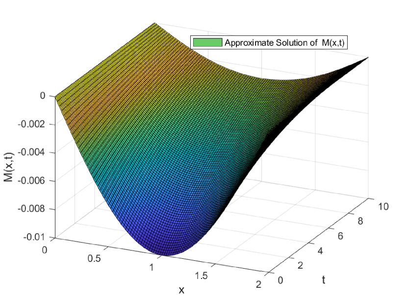
(a)

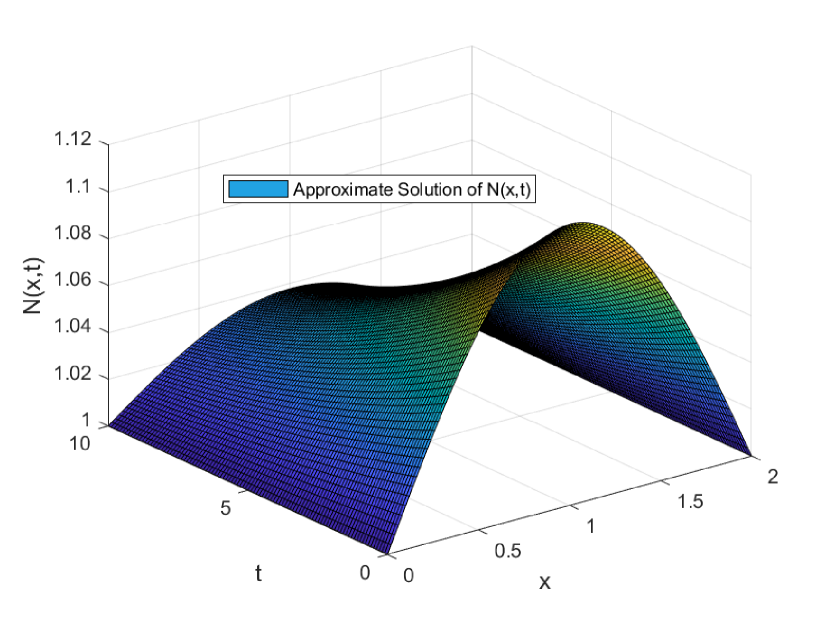
(b)

Figure 3.1: Approximate solution of $M(x,t)$ and $N(x,t)$ of (3.3) by using the present method for $(x,t)\in[0,2]\times[0,2]$

In Figure (3.1) we have employed a three-dimensional graphical depiction of approximate solutions of $M(x,t)$ and $N(x,t)$ at different time levels for better understanding. The graphical representations agree with the results that we have obtained in the tables. Eventually, it makes sense clearly that the method is more applicable to solving such nonlinear parabolic PDE systems.
In Figure (3.2), we have presented the error graph of $M(x,t)$ and $N(x,t)$ at time $t=10$, where the absolute errors are computed between two different time increments, say $\Delta t=0.2$, $\Delta t=0.4$ and $\Delta t=0.1$, $\Delta t=0.2$.

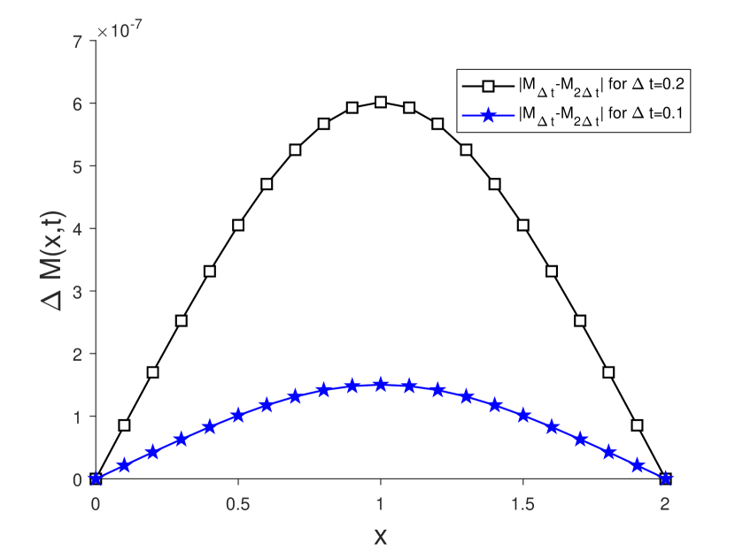
(a)

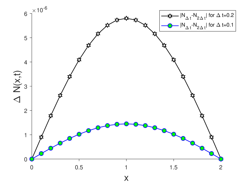
(b)

Figure 3.2: Absolute error of $M(x,t)$ and $N(x,t)$ from equation (3.3) for different time increment at time $t=10$.

The $L_{2}$ norm and $L_{\infty}$ norm, are presented in Table (3.3), which shows that the comparative errors are reduced significantly according to the reduction of the size of the time increments.

Table 3.3: The $L_{2}$ and $L_{\infty}$ norm at $t=10$ for $M(x,t)$ of equation (3.3).

$\Delta t$	$M(x,t)$		$N(x,t)$
	$L_{2}$ norm	$L_{\infty}$ norm	$L_{2}$ norm	$L_{\infty}$ norm
0.40	-	-	-	-
0.20	0.00000138	0.00000060	0.00001359	0.00000580
0.10	0.00000035	0.00000015	0.00000340	0.00000145

Test Problem 2: The Gray-Scott Model is one of the most important models whose wave formations are similar to many waves formed in real life such as butterfly wings, gesticulation, damping, turning patterns, embryos, multiple spots, and so on [29, 46]. Let us consider the following model,

$$\left.\begin{array}[]{lcl}\displaystyle\frac{\partial M}{\partial t}=\varepsilon_{1}\frac{\partial^{2}M}{\partial x^{2}}-f(M,N)+p(1-M)\\ \displaystyle\frac{\partial N}{\partial t}=\varepsilon_{2}\frac{\partial^{2}N}{\partial x^{2}}+f(M,N)-(p+q)N\\ \end{array}\right\}$$ (3.12)

where $f(M,N)=MN^{2}$. The boundary conditions and the initial conditions are considered as follows:

$$\left.\begin{array}[]{lcl}\displaystyle M(-50,t)=M(50,t)=1\\ \displaystyle N(-50,t)=N(50,t)=0\\ \end{array}\right\}$$ (3.15)

and

$$\left.\begin{array}[]{lcl}\displaystyle M(x,0)=1-0.5sin^{100}(\pi(x-50)/100)\\ \displaystyle N(x,0)=0.25sin^{100}(\pi(x-50)/100)\\ \end{array}\right\}$$ (3.18)

The domain of the model is $[-50,50]$. The values of the parameters are taken as

$\varepsilon_{1}=1$, $\varepsilon_{2}=0.01$, $p=0.01$, $q=0.12$

Here for computational purposes, we have used $7$ modified Bernstein polynomials. By applying the modified Galerkin method, we have used the backward difference method to transform the system of ordinary differential equations into the recurrent relations which is therefore solved by Picard iterative procedure. Numerical data of $M(x,t)$ and $N(x,t)$ of (3.3) are also presented in tabulated form in the following table at different time steps.

Table 3.4: Numerical results of concentrations $M(x,t)$ and $N(x,t)$ ate different time levels with $\Delta t=0.1$ and first 7 modified Bernstein polynomials.

x	$M(x,t)$			$N(x,t)$
	$t=1$	$t=10$	$t=20$	$t=1$	$t=10$	$t=20$
-50.0	1.0000	1.0000	1.0000	0.0000	0.0000	0.0000
-40.0	0.9725	0.9746	0.9767	0.0140	0.0164	0.0209
-30.0	1.0155	1.0201	1.0192	-0.0071	-0.0072	-0.0094
-20.0	1.0288	1.0056	0.9866	-0.0144	-0.0073	-0.0061
-10.0	0.8770	0.8515	0.8284	0.0623	0.0850	0.1148
0.0	0.7753	0.7563	0.7355	0.1139	0.1447	0.1922
10.0	0.8770	0.8515	0.8284	0.0623	0.0850	0.1148
20.0	1.0288	1.0056	0.9866	-0.0144	-0.0073	-0.0061
30.0	1.0155	1.0201	1.0192	-0.0071	-0.0072	-0.0094
40.0	0.9725	0.9746	0.9767	0.0140	0.0164	0.0209
50.0	1.0000	1.0000	1.0000	0.0000	0.0000	0.0000

The table shows that the numerical values of concentrations $M$ and $N$ change very slowly with varying values of $x$. It happens in every time step.

The results obtained by applying our proposed scheme are presented in Figure (3.3).

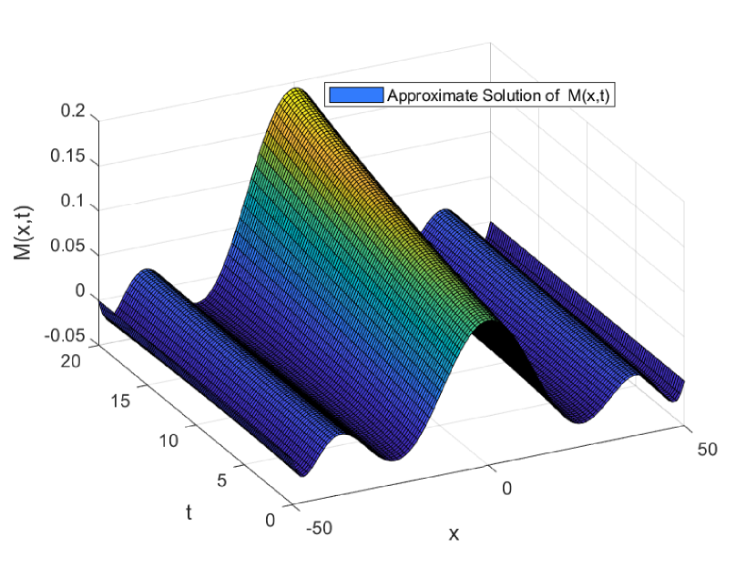
(a)

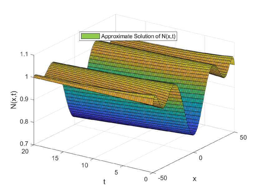
(b)

Figure 3.3: Absolute errors of $M(x,t)$ and $N(x,t)$ of (3.12) by using the present method for $(x,t)\in[-50,50]\times[0,20]$

Figure (3.3) is deployed to provide pictorial representations of the numerical concentrations $M$ and $N$ at different time levels. The results that are obtained in the table are shown graphically. The graphs are obtained for different time levels. The graphical presentation shows that the changes in concentrations are sufficiently small for different time levels.

The $L_{2}$ norm, and $L_{\infty}$ norms, are presented in table (3.5), which shows that the comparative errors are reduced significantly according to the reduction of the size of the time increments. However, the order of convergences increased noticeably along with the reduction of the time length.

Table 3.5: The $L_{2}$ and $L_{\infty}$ norm at $t=10$ for $M(x,t)$ of equation (3.12).

$\Delta t$	$M(x,t)$		$N(x,t)$
	$L_{2}$ norm	$L_{\infty}$ norm	$L_{2}$ norm	$L_{\infty}$ norm
0.40	-	-	-	-
0.20	0.00110596	0.00080091	0.00105161	0.00051358
0.10	0.00055524	0.00040251	0.00052415	0.00025600

In Figure (3.4), we have presented the error graph of $M(x,t)$ and $N(x,t)$ at time $t=10$, where the absolute errors are computed between two different time increments say $\Delta t=0.2$, $\Delta t=0.4$ and $\Delta t=0.1$, $\Delta t=0.2$.

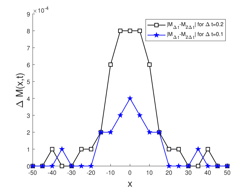
(a)

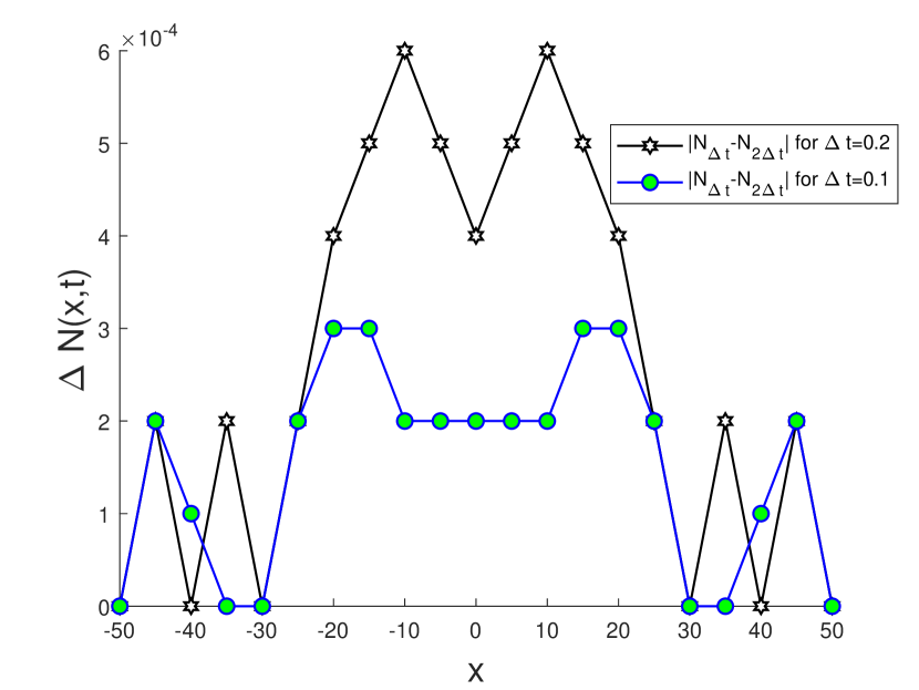
(b)

Figure 3.4: Approximate solution of $M(x,t)$ and $N(x,t)$ of (3.3) by using the present method for $(x,t)\in[0,2]\times[0,2]$

Conclusion

This research study has provided numerical approximations of nonlinear reaction-diffusion systems with specified boundary and initial conditions through the employment of the modified Galerkin method. To generate the trial solution, modified Bernstein Polynomials have been used. The simplification of the weighted residual leads to a system of ordinary differential equations which is then transformed into the recurrent relation by applying the backward difference formula. At this stage, we have used Picard’s iterative procedure to approximate the trial solution. After successful derivation, we applied our proposed method to several models in order to test their applicability and effectiveness. We have solved and displayed the results both numerically and graphically. From those figures and numerical results, it is indisputable that our proposed method is an unconditionally stable, efficient, highly modular, and easily expandable method that can be applied to any type of system of nonlinear parabolic partial differential equations regardless of the type of the boundary conditions, type of non-linearity of the functions, coefficients are constants or function of independent variables.

References

- [1] Biancalani, T., Fanelli, D., & Di Patti, F., (2010). Stochastic Turing patterns in the Brusselator model. Physical Review E, 81(4), 046215.
- [2] Wazwaz, A.-M.(2000). The decomposition method applied to systems of partial differential equations and to the reaction-diffusion Brusselator model. Applied mathematics and computation, 110(2-3).,251-264.
- [3] Muhammad Khan, F., Ali, A., Shah, K., Khan, A., Mahariq, I., et al. (2022). Analytical Approximation of Brusselator Model via LADM. Mathematical Problems in Engineering,2022, 01-14.
- [4] Alfifi, H. Y., Feedback control for a diffusive and delayed Brusselator model: Semi-analytical solutions. Symmetry, 13(4), 725.
- [5] Din, Q. (2018). A novel chaos control strategy for discrete-time Brusselator models. Journal of Mathematical Chemistry, 56(10), 3045-3075.
- [6] Ahmed, N., SS, T., Imran, M., Rafiq, M., Rehman, M., & Younis, M. (2019). Numerical analysis of auto-catalytic glycolysis model. AIP Advances, 9(8), 085213.
- [7] Ouannas, A., Batiha, I. M., Bekiros, S., Liu, J., Jahanshahi, H., Aly, A. A. & Alghtani, A. H. (2021). Synchronization of the glycolysis reaction-diffusion model via linear control law. Entropy, 23(11), 1516.
- [8] Iron, D., Wei, J., & Winter, M. (2004). Stability analysis of Turing patterns generated by the Schnakenberg model. Journal of mathematical biology, 49(4), 358-390.
- [9] Liu, P., Shi, J., Wang, Y., and Feng, X. (2013). Bifurcation analysis of reaction-diffusion Schnakenberg model. Journal of Mathematical Chemistry, 51(8),2001-2019.
- [10] Khan, F. M., Ali, A., Hamadneh, N., Abdullah & Alam, M. N. (2021). Numerical Investigation of Chemical Schnakenberg Mathematical Model. Journal of Nanomaterials, 2021, 1-8.
- [11] Beentjes, C. H. (2015). Pattern formation analysis in the Schnakenberg model (tech. rep.). Technical Report, University of Oxford, UK.
- [12] Gray, P. & Scott, S.(1983). Autocatalytic reactions in the isothermal, continuous stirred tank reactor: isolas and other forms of multistability. Chemical Engineering Science, 38(1), 29-43.
- [13] Sel’Kov, E. (1968). Self-Oscillations in Glycolysis 1. A Simple Kinetic Model. European Journal of Biochemistry, 4(1), 79-86.
- [14] Pearson, J. E. (1993). Complex patterns in a simple system. Science, 261(5118), 189-192.
- [15] Mazin, W., Rasmussen, K., Mosekilde, E., Borckmans, P. & Dewel, G. (1996). Pattern formation in the bistable Gray-Scott model. Mathematics and Computers in Simulation, 40(3-4), 371-396.
- [16] Doelman, A., Kaper, T. J., & Zegeling, P. A. (1997). Pattern formation in the one-dimensional Gray-Scott model. Nonlinearity, 10(2), 523.
- [17] Ueyama, D. (1999). Dynamics of self-replicating patterns in the one-dimensional Gray-Scott model. Hokkaido mathematical journal, 28(1), 175-210.
- [18] McGough, J. S. & Riley, K. (2004). Pattern formation in the Gray–Scott model. Nonlinear analysis: real world applications, 5(1), 105-121.
- [19] Doelman, A., Gardner, R., A., & Kaper, T., J. (1998). Stability analysis of singular patterns in the 1D Gray-Scott model: a matched asymptotics approach. Physica D: Nonlinear Phenomena, 122(1-4), 1-36.
- [20] Dkhil, F., Logak, E., & Nishiura, Y. (2004). Some analytical results on the Gray–Scott model. Asymptotic Analysis, 39(3-4), 225-261.
- [21] Nishiura, Y., & Ueyama, D. (2001). Spatio-temporal chaos for the Gray–Scott model. Physica D: Nonlinear Phenomena, 150(3-4), 137-162.
- [22] Nishiura, Y., & Ueyama, D. (2000). Self-replication, self-destruction, and spatio-temporal chaos in the Gray-Scott model. Physical Review Letters, 15(3), 281-289.
- [23] Wei, J. (2001). Pattern formations in two-dimensional Gray–Scott model: existence of single-spot solutions and their stability. Physica D: Nonlinear Phenomena, 148(1-2), 20-48.
- [24] Zhang, K., Wong, J. C.-F. & Zhang, R., (2008). Second-order implicit–explicit scheme for the Gray–Scott model. Journal of Computational and Applied Mathematics, 213(2), 559-581.
- [25] Mach, J. (2012). Application of the nonlinear Galerkin FEM method to the solution of the reaction diffusion equations.
- [26] Zhang, R., Zhu, J., Loula, A. F. & Yu, X. (2016). A new nonlinear Galerkin finite element method for the computation of reaction diffusion equations. Journal of Mathematical Analysis and Applications, 434(1), 136-148.
- [27] Mach, J. (2010). Quantitative analysis of numerical solution for the Gray-Scott model. SNA’10, 110.
- [28] Singh, S. (2023). Numerical investigation of wave pattern evolution in Gray–Scott model using discontinuous Galerkin finite element method. Advances in Mathematical and Computational Modeling of Engineering Systems, 47-58.
- [29] Tok-Onarcan, A., Adar, N., & Dag, I. (2019). Wave simulations of Gray-Scott reaction-diffusion system, 42(16), 5566-5581.
- [30] Owolabi, K. M. & Patidar, K. C. (2014). Numerical solution of singular patterns in one-dimensional Gray-Scott-like models. International Journal of Nonlinear Sciences and Numerical Simulation, 15(7-8), 437-462.
- [31] Kaur, N. & Joshi, V. (2022). Numerical solution to the Gray-Scott Reaction-Diffusion equation using Hyperbolic B-spline. Journal of Physics: Conference Series, 2267(1), 012072.
- [32] Thornton, A. & Marchant, T. R. (2008). Semi-analytical solutions for a Gray–Scott reaction–diffusion cell with an applied electric field. Chemical engineering science, 63(2), 495-502.
- [33] Chen, W., & Ward, M. J. (2011). The stability and dynamics of localized spot patterns in the two-dimensional Gray–Scott model. SIAM Journal on Applied Dynamical Systems, 10(2), 582-666.
- [34] Joshi, V. & Kaur, N. (2020). Numerical Solution of Gray Scott Reaction-Diffusion Equation using Lagrange Polynomial. Journal of Physics: Conference Series, 1531(1), 012058.
- [35] Che, H., Wang, Y.-L., & Li, Z.-Y. (2022). Novel patterns in a class of fractional reaction–diffusion models with the Riesz fractional derivative. Mathematics and Computers in Simulation, 202, 149-163.
- [36] Mittal, R., Kumar, S. & Jiwari, R. (2022). A cubic B-spline quasi-interpolation algorithm to capture the pattern formation of coupled reaction-diffusion models. Engineering with Computers, 38(2), 1375-1391.
- [37] Lewis, P. E. & Ward, J. P. (1991). The finite element method: principles and applications, Addison-Wesley Wokingham.
- [38] Hossan, M. S., Hossain, A. S. & Islam, M. S. (2020). Numerical Solutions of Black-Scholes Model by Du Fort-Frankel FDM and Galerkin WRM. International Journal of Mathematical Research, 9(1), 1-10.
- [39] Shirin, A., Islam, M., et al. (2013). Numerical solutions of Fredholm integral equations using Bernstein polynomials. arXiv preprint arXiv:1309.6311.
- [40] Cicelia, J. E. (2014). Solution of weighted residual problems by using Galerkin’s method. Indian Journal of Science and Technology, 7(3), 52-54.
- [41] Farzana, H., Islam, M. S., & Bhowmik, S. K. (2015). Computation of eigenvalues of the fourth order Sturm-Liouville BVP by Galerkin weighted residual method. British Journal of Mathematics and Computer Science, 9, 73-85.
- [42] Kang, Z., Wang, Z., Zhou, B. & Xue, S. (2020). Galerkin weighted residual method for axially functionally graded shape memory alloy beams. Journal of Mechanics, 36(3), 331-345.
- [43] Arani, A. A. A., Arefmanesh, A., & Niroumand, A. (2018). Investigation of fully developed flow and heat transfer through n-sided polygonal ducts with round corners using the Galerkin weighted residual method. Int. J. Nonlinear Anal. Appl, 9(1), 175-193.
- [44] Temam, R. (2012). Infinite-dimensional dynamical systems in mechanics and physics (Vol. 68). Springer Science & Business Media.
- [45] Manaa, S. A., Rasheed, J. (2013). Successive and finite difference method for Gray Scott model. Science Journal of University of Zakho, 1(2), 862-873.
- [46] Jiwari, R., Singh, S., & Kumar, A. (2017). Numerical simulation to capture the pattern formation of coupled reaction-diffusion models. Chaos, Solitons & Fractals, 103, 422-439.