An implicit DG solver for incompressible two-phase flows with an artificial compressibility formulation

Abstract

We propose an implicit Discontinuous Galerkin (DG) discretization for incompressible two-phase flows using an artificial compressibility formulation. Conservative level set (CLS) method is employed in combination with a reinitialization procedure to capture the moving interface. A projection method based on the L-stable TR-BDF2 method is adopted for the time discretization of the Navier-Stokes equations and of the level set method. Adaptive Mesh Refinement (AMR) is employed to enhance the resolution in correspondence of the interface between the two fluids. The effectiveness of the proposed approach is shown in a number of classical benchmarks, such as the Rayleigh-Taylor instability and the rising bubble test case, for which a specific analysis on the influence of different choices of the mixture viscosity is carried out.

⁽¹⁾ MOX - Dipartimento di Matematica, Politecnico di Milano
Piazza Leonardo da Vinci 32, 20133 Milano, Italy
giuseppe.orlando@polimi.it

Keywords: Navier-Stokes equations, incompressible flows, two-phase flows, artificial compressibility, Discontinuous Galerkin methods.

1 Introduction

Two-phase flows are common in many engineering and industrial applications. An evolving interface delimits the bulk regions of the single phases. Many techniques have been developed over the years to capture the motion of the interface. Two classes of methods are commonly used to locate the interface: interface-tracking and interface-capturing. Interface-tracking schemes employ either Arbitrary Lagrangian–Eulerian (ALE) methods on a mesh that deforms with the interface [15, 26] or marker and cell methods [44]. Interface-capturing techniques are instead based on fixed spatial grids with an interface function which captures the interface. A full survey on interface-capturing methods goes beyond the scope of this work and we refer e.g. to [32] for a review of these techniques. Interface capturing methods include the level set (LS) method [38, 39], which represents the interface as an iso-surface of the so-called level set function. Classically, the level set function is defined as the signed distance function. However, this choice leads to non conservative methods. A number of approaches have been developed to overcome this issue; in this work, we employ the conservative level set (CLS) method, originally proposed in [34, 33], and briefly summarized in Section 2.2. CLS includes a reinitialization equation to maintain the shape of the level set, which will be also discussed in Section 2.2.
Changing fluid properties, such as density and viscosity, and surface tension at the interface lead to discontinuities that make the discretization of the Navier-Stokes equations particularly challenging. The Discontinuous Galerkin (DG) method has been widely employed in the field of Computational Fluid Dynamics, see e.g. [8, 20, 28], and is a natural candidate for the discretization of the governing equations of two-phase flows. Several approaches have been proposed in the literature combining the DG method and the level set method, see among many others [21, 22, 40, 41]. In this paper, we propose an extension of the solver for single-phase incompressible Navier-Stokes equations with an artificial compressibility formulation presented in [35, 37], so as to overcome well know issues of projection methods. The time discretization is therefore based on the TR-BDF2 scheme [4, 9, 25, 37], which is a second order two-stage method. A brief review of the TR-BDF2 method will be given in Section 3, whereas we refer to [9, 25] for a detailed analysis of the scheme. The solver is implemented in the framework of the open source numerical library deal.II [2], which supports native non-conforming $h-$adaptation. We will exploit these capabilities to enhance the resolution in the regions close to the interface between the two fluids.
The paper is structured as follows: the model equations and their non-dimensional formulation are reviewed in Section 2. The time discretization approach is outlined and discussed in Section 3. The spatial discretization is presented in Section 4. The application of the proposed method to a number of significant benchmarks is reported in Section 5. Here, we also analyze the impact of different possible choices for the mixture viscosity when the interface undergoes large deformations. Finally, some conclusions and perspectives for future work are presented in Section 6.

2 The model equations

Let $\Omega\subset\mathbb{R}^{d},2\leq d\leq 3$ be a connected open bounded set with a sufficiently smooth boundary $\partial\Omega$ and denote by $\mathbf{x}$ the spatial coordinates and by $t$ the temporal coordinate. The two fluids in $\Omega$ are considered immiscible and they are contained in the subdomains $\Omega_{1}(t)$ and $\Omega_{2}(t)$, respectively, so that $\overline{\Omega_{1}(t)}\cup\overline{\Omega_{2}(t)}=\overline{\Omega}$. The moving interface between the two fluids is denoted by $\Gamma(t)$, defined as $\Gamma(t)=\partial\Omega_{1}(t)\cap\partial\Omega_{2}(t)$. We consider the classical unsteady, isothermal, incompressible Navier-Stokes equations with gravity, which read as follows [27]:

$$\rho(\mathbf{x})\left[\frac{\partial\mathbf{u}}{\partial t}+\left(\mathbf{u}\cdot\nabla\right)\mathbf{u}\right] = -\nabla p+\operatorname{\nabla\cdot}\left[2\mu(\mathbf{x})\mathbf{D}(\mathbf{u})\right]+\rho(\mathbf{x})\mathbf{g}$$

$$\operatorname{\nabla\cdot}\mathbf{u} = 0,$$ (1)

for $\mathbf{x}\in\Omega$, $t\in(0,T_{f}]$, supplied with suitable initial and boundary conditions. Here $T_{f}$ is the final time, $\mathbf{u}$ is the fluid velocity, $p$ is the pressure, $\rho$ is the fluid density and $\mu$ is the dynamic viscosity. We assume that both the density and the viscosity are discontinuous functions

$$\rho(\mathbf{x})=\begin{cases}\rho_{1}\quad\text{in }\Omega_{1}(t)\\ \rho_{2}\quad\text{in }\Omega_{2}(t)\\ \end{cases}\qquad\text{and}\qquad\mu(\mathbf{x})=\begin{cases}\mu_{1}\quad\text{in }\Omega_{1}(t)\\ \mu_{2}\quad\text{in }\Omega_{2}(t)\\ \end{cases}$$ (2)

with $\rho_{1},\rho_{2},\mu_{1},$ and $\mu_{2}$ constant values. Moreover, $\mathbf{g}$ is the gravitational acceleration and $\mathbf{D}(\mathbf{u})$ denotes the symmetric part of the gradient of the velocity, defined as

$$\mathbf{D}(\mathbf{u})=\frac{1}{2}\left[\nabla\mathbf{u}+\left(\nabla\mathbf{u}\right)^{T}\right].$$ (3)

In the following, for the sake of simplicity in the notation, we omit the explicit dependence on space and time for the different quantities. Surface tension effects are taken into accounts through the following balance of forces at the interface $\Gamma$:

$$\left[\mathbf{u}\right]_{\Gamma}=\mathbf{0}\qquad\left[-p\mathbf{I}+2\mu\mathbf{D}(\mathbf{u})\right]_{\Gamma}\mathbf{n}_{\Gamma}=\sigma\kappa\mathbf{n}_{\Gamma},$$ (4)

where $\mathbf{n}_{\Gamma}$ is the outward unit normal to $\Gamma$, $\left[\Psi\right]_{\Gamma}=\Psi\rvert_{\Gamma\cap\Omega_{1}}-\Psi\rvert_{\Gamma\cap\Omega_{2}}$ denotes the jump of $\Psi$ across the interface $\Gamma$, $\sigma$ is the constant surface tension coefficient, and $\kappa=-\operatorname{\nabla\cdot}\mathbf{n}_{\Gamma}$ is the curvature. The first condition implies the continuity of the velocity along $\Gamma$, whereas the second condition describes the balance of forces at the interface. A common way to handle the term with surface tension is to introduce the following volumetric force [27]:

$$\mathbf{f}_{\sigma}=\sigma\kappa\mathbf{n}_{\Gamma}\delta(\Gamma),$$ (5)

where $\delta(\Gamma)$ is the Dirac delta distribution supported on the interface. Hence, system (2) can be rewritten as follows:

$$\rho\left[\frac{\partial\mathbf{u}}{\partial t}+\left(\mathbf{u}\cdot\nabla\right)\mathbf{u}\right] = -\nabla p+\operatorname{\nabla\cdot}\left[2\mu\mathbf{D}(\mathbf{u})\right]+\rho\mathbf{g}+\mathbf{f}_{\sigma}$$

$$\operatorname{\nabla\cdot}\mathbf{u} = 0.$$ (6)

A level set approach [38, 49] is employed to capture the interface $\Gamma$. The interface between the two fluids is considered sharp and is described as the zero level set of a smooth function. Hence, the following relation holds:

$$\frac{\partial\varphi}{\partial t}+\mathbf{u}\cdot\nabla\varphi=0,$$ (7)

where $\varphi$ is the level set function. A common choice [49] is to consider as level set the signed distance function to $\Gamma$. In order to fix the notation, we consider $\varphi<0$ in $\Omega_{2}$ and $\varphi>0$ in $\Omega_{1}$. Therefore, we define

$$\varphi=\begin{cases}-\text{dist}(\mathbf{x},\Gamma)\qquad&\text{if }\mathbf{x}\in\Omega_{2}\\ 0&\text{if }\mathbf{x}\in\Gamma\\ \text{dist}(\mathbf{x},\Gamma)\qquad&\text{if }\mathbf{x}\in\Omega_{1}\\ \end{cases}$$ (8)

The unit normal vector can be evaluated at each point as follows [16, 38]:

$$\mathbf{n}_{\Gamma}=\frac{\nabla\varphi}{\left|\nabla\varphi\right|},\qquad\mathbf{x}\in\Gamma,$$ (9)

so that (7) is equivalent to

$$\frac{\partial\varphi}{\partial t}+\left(\mathbf{u}\cdot\mathbf{n}_{\Gamma}\right)\left|\nabla\varphi\right|=0.$$ (10)

Relation (10) shows that the deformation of the level set function is due only to the normal component of the velocity. Moreover, we can express the density and the dynamic viscosity through the Heaviside function $H$

$$\rho = \rho_{2}+\left(\rho_{1}-\rho_{2}\right)H(\varphi)$$ (11)

$$\mu = \mu_{2}+\left(\mu_{1}-\mu_{2}\right)H(\varphi)$$ (12)

The whole system of equations reads therefore as follows:

$$\rho\left[\frac{\partial\mathbf{u}}{\partial t}+\left(\mathbf{u}\cdot\nabla\right)\mathbf{u}\right] = -\nabla p+\operatorname{\nabla\cdot}\left[2\mu\mathbf{D}(\mathbf{u})\right]+\rho\mathbf{g}+\mathbf{f}_{\sigma}$$

$$\operatorname{\nabla\cdot}\mathbf{u} = 0$$ (13)

$$\frac{\partial\varphi}{\partial t}+\mathbf{u}\cdot\nabla\varphi = 0.$$

System (2) can be rewritten in conservative form. First of all, thanks to the incompressibility constraint $\operatorname{\nabla\cdot}\mathbf{u}=0$, we can rewrite (7) as

$$\frac{\partial\varphi}{\partial t}+\operatorname{\nabla\cdot}\left(\varphi\mathbf{u}\right)=0.$$ (14)

Moreover, one can verify that (7), in combination with the incompressibility constraint, implies mass conservation. Indeed, we get

$$\frac{\partial\rho}{\partial t}+\operatorname{\nabla\cdot}\left(\rho\mathbf{u}\right)=\frac{\partial\rho}{\partial t}+\mathbf{u}\cdot\nabla\rho = \left(\rho_{1}-\rho_{2}\right)\left(\frac{\partial H(\varphi)}{\partial t}+\mathbf{u}\cdot\nabla H(\varphi)\right)$$ (15)

$$= \left(\rho_{1}-\rho_{2}\right)\delta(\varphi)\left(\frac{\partial\varphi}{\partial t}+\mathbf{u}\cdot\nabla\varphi\right)=0,$$

where we exploited the relation $\frac{dH(\varphi)}{d\varphi}=\delta(\varphi)$ [46], with $\delta(\varphi)$ denoting the Dirac delta distribution with support equal to the function $\varphi$ which implicitly describes the surface. It is appropriate to stress the fact that the differential operators involving the Heaviside function $H(\varphi)$ have to be intended in a proper distributional sense. Finally, as discussed in [30], we can rewrite

$$\mathbf{f}_{\sigma}=\operatorname{\nabla\cdot}\left[\sigma\left(\mathbf{I}-\mathbf{n}_{\Gamma}\otimes\mathbf{n}_{\Gamma}\right)\delta(\Gamma)\right],$$ (16)

where, once more, the divergence operator should be intended in a distributional sense. Hence, the conservative form of (2) is

$$\frac{\partial\left(\rho\mathbf{u}\right)}{\partial t}+\operatorname{\nabla\cdot}\left(\rho\mathbf{u}\otimes\mathbf{u}\right) = -\nabla p+\operatorname{\nabla\cdot}\left[2\mu\mathbf{D}(\mathbf{u})\right]+\rho\mathbf{g}+\mathbf{f}_{\sigma}$$

$$\operatorname{\nabla\cdot}\mathbf{u} = 0$$ (17)

$$\frac{\partial\varphi}{\partial t}+\operatorname{\nabla\cdot}\left(\varphi\mathbf{u}\right) = 0.$$

The Continuum Surface Force (CSF) approach, introduced in [10], is employed to treat density, viscosity, and surface tension term. A regularized Heaviside $H_{\varepsilon}(\varphi)$ is introduced, so as to obtain

$$\rho\approx\rho_{2}+\left(\rho_{1}-\rho_{2}\right)H_{\varepsilon}(\varphi)$$ (18)

$$\mu\approx\mu_{2}+\left(\mu_{1}-\mu_{2}\right)H_{\varepsilon}(\varphi).$$ (19)

It is important at this stage to point out the relation between $\delta(\Gamma)$ and $\delta(\varphi)$. As discussed in [17], the following relation holds:

$$\delta(\Gamma)=\delta(\varphi)\left|\nabla\varphi\right|,$$ (20)

so that we can rewrite

$$\mathbf{f}_{\sigma}=\sigma\kappa\mathbf{n}_{\Gamma}\delta(\varphi)\left|\nabla\varphi\right|=\operatorname{\nabla\cdot}\left[\sigma\left(\mathbf{I}-\mathbf{n}_{\Gamma}\otimes\mathbf{n}_{\Gamma}\right)\delta(\varphi)\left|\nabla\varphi\right|\right].$$ (21)

Hence, the CSF approximation of the surface tension term reads as follows:

$$\mathbf{f}_{\sigma}\approx\operatorname{\nabla\cdot}\left[\sigma\left(\mathbf{I}-\mathbf{n}_{\Gamma}\otimes\mathbf{n}_{\Gamma}\right)\delta_{\varepsilon}(\varphi)\left|\nabla\varphi\right|\right]=\operatorname{\nabla\cdot}\left[\sigma\left(\mathbf{I}-\mathbf{n}_{\Gamma}\otimes\mathbf{n}_{\Gamma}\right)\frac{dH_{\varepsilon}}{d\varphi}(\varphi)\left|\nabla\varphi\right|\right].$$ (22)

Since the seminal proposals in [13, 50] (see also the review in [23]), projection methods have become very popular for the discretization of incompressible Navier-Stokes equations. However, difficulties arise in choosing boundary conditions for the Poisson equation which is to be solved at each time step to compute the pressure. An alternative that allows to avoid or reduce some of these problems is the so-called artificial compressibility formulation, originally introduced in [12] and employed in [7, 37] among many others. In this formulation, the incompressibility constraint is relaxed and a time evolution equation for the pressure is introduced. This kind of approach has been adopted for incompressible flows with variable density, see e.g. [6, 31], and we aim here to consider an artificial compressibility formulation for immiscible, isothermal two-phase flows with gravity. The model equations can be therefore rewritten as follows:

$$\frac{\partial\left(\rho\mathbf{u}\right)}{\partial t}+\operatorname{\nabla\cdot}\left(\rho\mathbf{u}\otimes\mathbf{u}\right) = -\nabla p+\operatorname{\nabla\cdot}\left[2\mu\mathbf{D}(\mathbf{u})\right]+\rho\mathbf{g}+\mathbf{f}_{\sigma}$$

$$\frac{1}{\rho_{0}c^{2}}\frac{\partial p}{\partial t}+\operatorname{\nabla\cdot}\mathbf{u} = 0$$ (23)

$$\frac{\partial\varphi}{\partial t}+\operatorname{\nabla\cdot}\left(\varphi\mathbf{u}\right) = 0,$$

where $c$ is the artificial speed of sound and $\rho_{0}$ is a reference density. Finally, since we are relaxing the incompressibility constraint, we consider (7) for the level set motion, which is valid for the transport of $\varphi$ independently of the constraints on the velocity $\mathbf{u}$. Moreover, this choice is justified by the results reported in [35] for a rising bubble test case, for which a non-conservative formulation leads to less diffusion in the treatment of the interface. Hence, the final form of the system under consideration reads as follows:

$$\frac{\partial\left(\rho\mathbf{u}\right)}{\partial t}+\operatorname{\nabla\cdot}\left(\rho\mathbf{u}\otimes\mathbf{u}\right) = -\nabla p+\operatorname{\nabla\cdot}\left[2\mu\mathbf{D}(\mathbf{u})\right]+\rho\mathbf{g}+\mathbf{f}_{\sigma}$$

$$\frac{1}{\rho_{0}c^{2}}\frac{\partial p}{\partial t}+\operatorname{\nabla\cdot}\mathbf{u} = 0$$ (24)

$$\frac{\partial\varphi}{\partial t}+\mathbf{u}\cdot\nabla\varphi = 0,$$

Before proceeding to describe the time and space discretization schemes, we perform a dimensional analysis to derive a non-dimensional version of system (2).

2.1 Dimensional analysis

In this Section, we derive a non-dimensional formulation for system (2). We denote with the symbol $*$ non-dimensional quantities. We introduce a reference length and velocity, denoted by $L_{ref}$ and $U_{ref}$, respectively, so as to obtain

$$\mathbf{x}=L_{ref}\mathbf{x}^{*}\qquad\mathbf{u}=U_{ref}\mathbf{u}^{*}\qquad t=\frac{L_{ref}}{U_{ref}}t^{*}.$$ (25)

Moreover, we choose as reference density and viscosity those associated to the heavier fluid, which is conventionally considered in $\Omega_{1}$. For the sake of simplicity, we also assume $\rho_{0}=\rho_{1}$. The reference pressure $p_{ref}$ is taken equal to $p_{ref}=\rho_{1}U_{ref}^{2}$. Hence, we get

$$\rho=\rho_{1}\rho^{*}\qquad\mu=\mu_{1}\mu^{*}\qquad p=\rho_{1}U_{ref}^{2}p^{*}\qquad\kappa=\frac{1}{L_{ref}}\kappa^{*}\qquad\varphi=L_{ref}\varphi^{*}.$$ (26)

Introducing the appropriate non-dimensional quantities, we obtain

$$\frac{\rho_{1}U_{ref}^{2}}{L_{ref}}\frac{\partial^{*}\left(\rho^{*}\mathbf{u}^{*}\right)}{\partial^{*}t^{*}}+\frac{\rho_{1}U_{ref}^{2}}{L_{ref}}\nabla^{*}\cdot\left(\rho^{*}\mathbf{u}^{*}\otimes\mathbf{u}^{*}\right) = -\frac{\rho_{1}U_{ref}^{2}}{L_{ref}}\nabla^{*}p^{*}+\frac{\mu_{1}U_{ref}}{L_{ref}}\nabla^{*}\cdot\left[2\mu^{*}\mathbf{D}(\mathbf{u}^{*})\right]$$

$$- \rho_{1}\rho^{*}g\mathbf{k}$$

$$+ \frac{1}{L_{ref}^{2}}\nabla^{*}\cdot\left[\sigma\left(\mathbf{I}-\mathbf{n}_{\Gamma}\otimes\mathbf{n}_{\Gamma}\right)\delta^{*}_{\varepsilon}(\varphi^{*})\left|\nabla^{*}\varphi^{*}\right|\right]$$

$$\frac{\rho_{1}U_{ref}^{3}}{\rho_{1}L_{ref}}\frac{1}{c^{2}}\frac{\partial^{*}p^{*}}{\partial^{*}t^{*}}+\frac{U_{ref}}{L_{ref}}\nabla^{*}\cdot\mathbf{u}^{*} = 0$$ (27)

$$U_{ref}\frac{\partial^{*}\varphi^{*}}{\partial^{*}t^{*}}+U_{ref}\mathbf{u}^{*}\cdot\nabla^{*}\varphi^{*} = 0,$$

where $\mathbf{k}$ is the upward pointing unit vector in the standard Cartesian reference frame. System (2.1) reduces to

$$\frac{\partial^{*}\left(\rho^{*}\mathbf{u}^{*}\right)}{\partial^{*}t^{*}}+\nabla^{*}\cdot\left(\rho^{*}\mathbf{u}^{*}\otimes\mathbf{u}^{*}\right) = -\nabla^{*}p^{*}+\frac{1}{Re}\nabla^{*}\cdot\left[2\mu^{*}\mathbf{D}(\mathbf{u}^{*})\right]$$

$$- \frac{1}{Fr^{2}}\rho^{*}\mathbf{k}$$

$$+ \frac{1}{We}\nabla^{*}\cdot\left[\left(\mathbf{I}-\mathbf{n}_{\Gamma}\otimes\mathbf{n}_{\Gamma}\right)\delta^{*}_{\varepsilon}(\varphi^{*})\left|\nabla^{*}\varphi^{*}\right|\right]$$

$$M^{2}\frac{\partial^{*}p^{*}}{\partial^{*}t^{*}}+\nabla^{*}\cdot\mathbf{u}^{*} = 0$$ (28)

$$\frac{\partial^{*}\varphi^{*}}{\partial^{*}t^{*}}+\mathbf{u}^{*}\cdot\nabla^{*}\varphi^{*} = 0,$$

where

$$Re=\frac{\rho_{1}U_{ref}L_{ref}}{\mu_{1}}\qquad Fr=\frac{U_{ref}}{\sqrt{gL_{ref}}}\qquad We=\frac{\rho_{1}U_{ref}^{2}L_{ref}}{\sigma}\qquad M=\frac{U_{ref}}{c}$$ (29)

denote the Reynolds number, the Froude number, the Weber number, and the Mach number, respectively. In the following, with a slight abuse of notation, we omit the symbol $*$ to mark non-dimensional quantities and we consider therefore the following system of equations:

$$\frac{\partial\left(\rho\mathbf{u}\right)}{\partial t}+\operatorname{\nabla\cdot}\left(\rho\mathbf{u}\otimes\mathbf{u}\right) = -\nabla p+\frac{1}{Re}\operatorname{\nabla\cdot}\left[2\mu\mathbf{D}(\mathbf{u})\right]$$

$$- \frac{1}{Fr^{2}}\rho\mathbf{k}+\frac{1}{We}\operatorname{\nabla\cdot}\left[\left(\mathbf{I}-\mathbf{n}_{\Gamma}\otimes\mathbf{n}_{\Gamma}\right)\delta_{\varepsilon}(\varphi)\left|\nabla\varphi\right|\right]$$

$$M^{2}\frac{\partial p}{\partial t}+\operatorname{\nabla\cdot}\mathbf{u} = 0$$ (30)

$$\frac{\partial\varphi}{\partial t}+\mathbf{u}\cdot\nabla\varphi = 0,$$

where

$$\rho = \frac{\rho_{2}}{\rho_{1}}+\left(1-\frac{\rho_{2}}{\rho_{1}}\right)H_{\varepsilon}(\varphi)$$ (31)

$$\mu = \frac{\mu_{2}}{\mu_{1}}+\left(1-\frac{\mu_{2}}{\mu_{1}}\right)H_{\varepsilon}(\varphi).$$ (32)

2.2 The conservative level set method

The traditional level set method lacks of volume conservation properties [18]. The conservative level set (CLS) method [33, 34, 53] is a popular alternative to add conservation properties to level set schemes. The idea is to replace the signed distance function defined in (8) with a regularized Heaviside function:

$$\phi(\mathbf{x},t)=\frac{1}{1+e^{-\varphi(\mathbf{x},t)/\varepsilon}},$$ (33)

where $\varepsilon$ helps smoothing the transition of the discontinuous physical properties between the two subdomains and it is also known as interface thickness. Since

$$\nabla\phi=\frac{1}{\varepsilon}\frac{e^{-\varphi/\varepsilon}}{\left(1+e^{-\varphi/\varepsilon}\right)^{2}}\nabla\varphi$$ (34)

we can compute the outward unit normal $\mathbf{n}_{\Gamma}$ exactly as in (9). From definition (33), it follows that

$$\Gamma(t)=\left\{\mathbf{x}\in\overline{\Omega}:\phi(\mathbf{x},t)=\frac{1}{2}\right\}.$$ (35)

This new level set function needs to be reinitialized in order to keep the property of being a regularized Heaviside function [34]. This goal is achieved by solving the following PDE [33, 34]:

$$\frac{\partial\phi}{\partial\tau}+\operatorname{\nabla\cdot}\left(u_{c}\phi\left(1-\phi\right)\mathbf{n}_{\Gamma}\right)=\operatorname{\nabla\cdot}\left(\beta\varepsilon u_{c}\left(\nabla\phi\cdot\mathbf{n}_{\Gamma}\right)\mathbf{n}_{\Gamma}\right),$$ (36)

where $\tau$ is an artificial pseudo-time variable, $u_{c}$ is an artificial compression velocity, and $\beta$ is a constant. It is important to notice that $\mathbf{n}_{\Gamma}$ does not change during the reinizialization procedure, but is computed using the initial value of the level set function. The relation (36) has been originally introduced as an intermediate step between the level set advection and the Navier-Stokes equations to keep the shape of the profile [33] and to stabilize the advection [34]. Two fluxes are considered: a compression flux which acts where $0<\phi<1$ and in normal direction to the interface, represented by $u_{c}\phi\left(1-\phi\right)\mathbf{n}_{\Gamma}$, and a diffusion flux, represented by $\beta\varepsilon u_{c}\left(\nabla\phi\cdot\mathbf{n}_{\Gamma}\right)\mathbf{n}_{\Gamma}$. The reinitialization is crucial for the overall stability of the algorithm, but it also introduces errors in the solution [34, 40]. Hence, it is important to avoid unnecessary reinitialization. For this purpose, unlike the formulation proposed e.g. in [34] and [40], we introduce the coefficient $\beta$ to tune the amount of diffusion so as to keep it as small as possible. The choices for the different parameters will be specified in Section 5. Finally, we stress the fact that, in this method, we are already using a smooth version of Heaviside function so that

$$H_{\varepsilon} = \phi$$ (37)

$$\delta(\Gamma)\approx\frac{dH_{\varepsilon}}{d\phi}\left|\nabla\phi\right| = \left|\nabla\phi\right|$$ (38)

3 The time discretization

In this Section, we outline the time discretization strategy for system (2.1). Our goal here is to extend the projection method based on the TR-BDF2 scheme developed in [37]. We now briefly recall for the convenience of the reader the formulation of the TR-BDF2. This second order implicit method has been originally introduced in [4] as a combination of the Trapezoidal Rule (or Crank-Nicolson) method and of the Backward Differentiation Formula method of order 2 (BDF2). Let $\Delta t=T_{f}/N$ be a discrete time step and $t^{n}=n\Delta t,n=0,\dots,N$, be discrete time levels for a generic time dependent problem $\bm{u}^{\prime}=\mathcal{N}(\bm{u})$. Hence, the incremental form of the TR-BDF2 scheme can be described in terms of two stages, the first one from $t^{n}$ to $t^{n+\gamma}=t^{n}+\gamma\Delta t$, and the second one from $t^{n+\gamma}$ to $t^{n+1}$, as follows:

$$\frac{\bm{u}^{n+\gamma}-\bm{u}^{n}}{\gamma\Delta t} = \frac{1}{2}\mathcal{N}\left(\bm{u}^{n+\gamma}\right)+\frac{1}{2}\mathcal{N}\left(\bm{u}^{n}\right)$$ (39)

$$\frac{\bm{u}^{n+1}-\bm{u}^{n+\gamma}}{\left(1-\gamma\right)\Delta t} = \frac{1}{2-\gamma}\mathcal{N}\left(\bm{u}^{n+1}\right)+\frac{1-\gamma}{2\left(2-\gamma\right)}\mathcal{N}\left(\bm{u}^{n+\gamma}\right)+\frac{1-\gamma}{2\left(2-\gamma\right)}\mathcal{N}\left(\bm{u}^{n}\right).$$ (40)

Here, $\bm{u}^{n}$ denotes the approximation at time $n=0,\dots,N$. Notice that, in order to guarantee L-stability, one has to choose $\gamma=2-\sqrt{2}$ [25]. We refer to [9, 25] for a more exhaustive discussion on the TR-BDF2 method.

We start by considering the equation in system (2.1) associated to the level set. In order to avoid a full coupling with the Navier-Stokes equations, we perform a linearization in velocity, so that the first stage for the level set update reads as follows:

$$\frac{\phi^{n+\gamma}-\phi^{n}}{\gamma\Delta t}+\frac{1}{2}\mathbf{u}^{n+\frac{\gamma}{2}}\cdot\nabla\phi^{n+\gamma}=-\frac{1}{2}\mathbf{u}^{n+\frac{\gamma}{2}}\cdot\nabla\phi^{n},$$ (41)

where the approximation $\mathbf{u}^{n+\frac{\gamma}{2}}$ is defined by extrapolation as

$$\mathbf{u}^{n+\frac{\gamma}{2}}=\left(1+\frac{\gamma}{2\left(1-\gamma\right)}\right)\mathbf{u}^{n}-\frac{\gamma}{2\left(1-\gamma\right)}\mathbf{u}^{n-1}.$$ (42)

Following then the projection approach described in [14, 37] and applying (39), the momentum predictor equation for the first stage reads as follows:

$$\frac{\rho^{n+\gamma}\mathbf{u}^{n+\gamma,*}-\rho^{n}\mathbf{u}^{n}}{\gamma\Delta t}$$

$$+ \frac{1}{2}\operatorname{\nabla\cdot}\left(\rho^{n+\gamma}\mathbf{u}^{n+\gamma,*}\otimes\mathbf{u}^{n+\frac{\gamma}{2}}\right)-\frac{1}{2}\frac{1}{Re}\operatorname{\nabla\cdot}\left[2\mu^{n+\gamma}\mathbf{D}(\mathbf{u}^{n+\gamma,*})\right]=$$

$$- \frac{1}{2}\operatorname{\nabla\cdot}\left(\rho^{n}\mathbf{u}^{n}\otimes\mathbf{u}^{n+\frac{\gamma}{2}}\right)+\frac{1}{2}\frac{1}{Re}\operatorname{\nabla\cdot}\left[2\mu^{n}\mathbf{D}(\mathbf{u}^{n})\right]-\nabla p^{n}$$

$$+ \frac{1}{2}\frac{1}{We}\operatorname{\nabla\cdot}\left[\left(\mathbf{I}-\mathbf{n}_{\Gamma}^{n+\gamma}\otimes\mathbf{n}_{\Gamma}^{n+\gamma}\right)\delta_{\varepsilon}(\phi^{n+\gamma})\left|\nabla\phi^{n+\gamma}\right|\right]$$

$$+ \frac{1}{2}\frac{1}{We}\operatorname{\nabla\cdot}\left[\left(\mathbf{I}-\mathbf{n}_{\Gamma}^{n}\otimes\mathbf{n}_{\Gamma}^{n}\right)\delta_{\varepsilon}(\phi^{n})\left|\nabla\phi^{n}\right|\right]$$

$$- \frac{1}{2}\frac{1}{Fr^{2}}\rho^{n+\gamma}\mathbf{k}-\frac{1}{2}\frac{1}{Fr^{2}}\rho^{n}\mathbf{k}.$$

Notice once more that, in order to avoid solving a non-linear system at each time step, $\mathbf{u}^{n+\frac{\gamma}{2}}$ is employed in the momentum advection terms. We set then $\delta p^{n+\gamma}=p^{n+\gamma}-p^{n}$ and impose

$$\rho^{n+\gamma}\frac{\mathbf{u}^{n+\gamma}-\mathbf{u}^{n+\gamma,*}}{\gamma\Delta t}=-\nabla\delta p^{n+\gamma}$$

$$M^{2}\frac{\delta p^{n+\gamma}}{\gamma\Delta t}+\operatorname{\nabla\cdot}\mathbf{u}^{n+\gamma}=0.$$ (44)

Substituting the first equation into the second in (3), one obtains the Helmholtz equation

$$M^{2}\frac{\delta p^{n+\gamma}}{\gamma^{2}\Delta t^{2}}-\operatorname{\nabla\cdot}\left(\frac{\nabla\delta p^{n+\gamma}}{\rho^{n+\gamma}}\right)=-\frac{1}{\gamma\Delta t}\operatorname{\nabla\cdot}\mathbf{u}^{n+\gamma,*}.$$ (45)

Once this equation is solved, the final velocity update for the first stage is given by

$$\mathbf{u}^{n+\gamma}=\mathbf{u}^{n+\gamma,*}-\gamma\Delta t\frac{\nabla\delta p^{n+\gamma}}{\rho^{n+\gamma}}.$$ (46)

The second TR-BDF2 stage is performed in a similar manner applying (40). We first focus on the level set update:

$$\frac{\phi^{n+1}-\phi^{n+\gamma}}{\left(1-\gamma\right)\Delta t}+a_{33}\mathbf{u}^{n+\frac{3}{2}\gamma}\cdot\nabla\phi^{n+1}=-a_{32}\mathbf{u}^{n+\gamma}\cdot\nabla\phi^{n+\gamma}-a_{31}\mathbf{u}^{n}\cdot\nabla\phi^{n},$$ (47)

where

$$a_{31}=\frac{1-\gamma}{2\left(2-\gamma\right)}\qquad a_{32}=\frac{1-\gamma}{2\left(2-\gamma\right)}\qquad a_{33}=\frac{1}{2-\gamma}.$$ (48)

Again, in order to avoid a full coupling with the Navier-Stokes equations, an approximation is introduced in the advection term, so that $\mathbf{u}^{n+\frac{3}{2}\gamma}$ is defined by extrapolation as

$$\mathbf{u}^{n+\frac{3}{2}\gamma}=\left(1+\frac{1+\gamma}{\gamma}\right)\mathbf{u}^{n+\gamma}-\frac{1-\gamma}{\gamma}\mathbf{u}^{n}.$$ (49)

Then, we define the second momentum predictor:

$$\frac{\rho^{n+1}\mathbf{u}^{n+1,*}-\rho^{n+\gamma}\mathbf{u}^{n+\gamma}}{\left(1-\gamma\right)\Delta t}$$

$$+ a_{33}\operatorname{\nabla\cdot}\left(\rho^{n+1}\mathbf{u}^{n+1,*}\otimes\mathbf{u}^{n+\frac{3}{2}\gamma}\right)-a_{33}\frac{1}{Re}\operatorname{\nabla\cdot}\left[2\mu^{n+1}\mathbf{D}(\mathbf{u}^{n+1,*})\right]=$$

$$- a_{32}\operatorname{\nabla\cdot}\left(\rho^{n+\gamma}\mathbf{u}^{n+\gamma}\otimes\mathbf{u}^{n+\gamma}\right)+a_{32}\frac{1}{Re}\operatorname{\nabla\cdot}\left[2\mu^{n+\gamma}\mathbf{D}(\mathbf{u}^{n+\gamma})\right]$$

$$- a_{31}\operatorname{\nabla\cdot}\left(\rho^{n}\mathbf{u}^{n}\otimes\mathbf{u}^{n}\right)+a_{31}\frac{1}{Re}\operatorname{\nabla\cdot}\left[2\mu^{n}\mathbf{D}(\mathbf{u}^{n})\right]-\nabla p^{n+\gamma}$$

$$+ a_{33}\frac{1}{We}\operatorname{\nabla\cdot}\left[\left(\mathbf{I}-\mathbf{n}_{\Gamma}^{n+1}\otimes\mathbf{n}_{\Gamma}^{n+1}\right)\delta_{\varepsilon}(\phi^{n+1})\left|\nabla\phi^{n+1}\right|\right]$$

$$+ a_{32}\frac{1}{We}\operatorname{\nabla\cdot}\left[\left(\mathbf{I}-\mathbf{n}_{\Gamma}^{n+\gamma}\otimes\mathbf{n}_{\Gamma}^{n+\gamma}\right)\delta_{\varepsilon}(\phi^{n+\gamma})\left|\nabla\phi^{n+\gamma}\right|\right]$$

$$+ a_{31}\frac{1}{We}\operatorname{\nabla\cdot}\left[\left(\mathbf{I}-\mathbf{n}_{\Gamma}^{n}\otimes\mathbf{n}_{\Gamma}^{n}\right)\delta_{\varepsilon}(\phi^{n})\left|\nabla\phi^{n}\right|\right]$$

$$- a_{33}\frac{1}{Fr^{2}}\rho^{n+1}\mathbf{k}-a_{32}\frac{1}{Fr^{2}}\rho^{n+\gamma}\mathbf{k}-a_{31}\frac{1}{Fr^{2}}\rho^{n}\mathbf{k}.$$

Notice that $\mathbf{u}^{n+\frac{3}{2}\gamma}$ is employed in the non-linear momentum advection term. We set then $\delta p^{n+1}=p^{n+1}-p^{n+\gamma}$ and impose

$$\rho^{n+1}\frac{\mathbf{u}^{n+1}-\mathbf{u}^{n+1,*}}{(1-\gamma)\Delta t}=-\nabla\delta p^{n+1}$$

$$M^{2}\frac{\delta p^{n+1}}{(1-\gamma)\Delta t}+\operatorname{\nabla\cdot}\mathbf{u}^{n+1}=0.$$ (51)

Substituting the first equation into the second in (3), one obtains the Helmholtz equation

$$M^{2}\frac{\delta p^{n+1}}{(1-\gamma)^{2}\Delta t^{2}}-\operatorname{\nabla\cdot}\left(\frac{\nabla\delta p^{n+1}}{\rho^{n+1}}\right)=-\frac{1}{(1-\gamma)\Delta t}\operatorname{\nabla\cdot}\mathbf{u}^{n+1,*}.$$ (52)

The final velocity update then reads as follows:

$$\mathbf{u}^{n+1}=\mathbf{u}^{n+1,*}-(1-\gamma)\Delta t\frac{\nabla\delta p^{n+1}}{\rho^{n+1}}.$$ (53)

Finally, we focus on the reinitialization procedure described in Equation 36, which is performed after each stage of the level set update and before computing the momentum predictor. We consider an implicit treatment of the diffusion term $\operatorname{\nabla\cdot}\left(\beta\varepsilon u_{c}\left(\nabla\phi\cdot\mathbf{n}_{\Gamma}\right)\mathbf{n}_{\Gamma}\right)$ and a semi-implicit treatment of the compression term $u_{c}\operatorname{\nabla\cdot}\left(\phi\left(1-\phi\right)\mathbf{n}_{\Gamma}\right)$. Hence, the semi-discrete formulation reads as follows:

$$\frac{\phi^{k+1,*}-\phi^{k,*}}{\Delta\tau}+\operatorname{\nabla\cdot}\left(u_{c}\phi^{k+1,*}\left(1-\phi^{k,*}\right)\mathbf{n}_{\Gamma}\right)=\operatorname{\nabla\cdot}\left(\beta\varepsilon u_{c}\left(\nabla\phi^{k+1,*}\cdot\mathbf{n}_{\Gamma}\right)\mathbf{n}_{\Gamma}\right),$$ (54)

where $\Delta\tau$ is the pseudo time step. Moreover, $\phi^{0,*}=\phi^{n+\gamma}$ after the first TR-BDF2 stage and $\phi^{0,*}=\phi^{n+1}$ after the second TR-BDF2 stage. We recall once more that $\mathbf{n}_{\Gamma}=\frac{\nabla\phi^{0,*}}{\left|\nabla\phi^{0,*}\right|}$ and it does not change during the reinitialization. Following [40], we define the total reinitialization time $\tau_{fin}$ as a fraction of the time step $\Delta t$, namely

$$\tau_{fin}=\eta\Delta t.$$ (55)

$\eta=0$ corresponds to no reinitialization, whereas $\eta=1$ yields an amount of reinitialization which can modify the values of level set function of the same order of magnitude of which they have been modified during the previous advection step. For most applications, $\eta\approx 0.5$ seems to provide an appropriate amount of reinitialization [40]. A pseudo time step such that two to five reinitialization steps are performed typically ensures stable solutions and leads to the updated level set function [29].

4 The spatial discretization

For the spatial discretization, we consider discontinuous finite element approximations. We consider a decomposition of the domain $\Omega$ into a family of hexahedra $\mathcal{T}_{h}$ (quadrilaterals in the two-dimensional case) and denote each element by $K$. The skeleton $\mathcal{E}$ denotes the set of all element faces and $\mathcal{E}=\mathcal{E}^{I}\cup\mathcal{E}^{B}$, where $\mathcal{E}^{I}$ is the subset of interior faces and $\mathcal{E}^{B}$ is the subset of boundary faces. Suitable jump and average operators can then be defined as customary for finite element discretizations. A face $e\in\mathcal{E}^{I}$ shares two elements that we denote by $K^{+}$ with outward unit normal $\mathbf{n}^{+}$ and $K^{-}$ with outward unit normal $\mathbf{n}^{-}$, whereas for a face $e\in\mathcal{E}^{B}$ we denote by $\mathbf{n}$ the outward unit normal. For a scalar function $\Psi$ the jump is defined as

$$\left[\left[\Psi\right]\right]=\Psi^{+}\mathbf{n}^{+}+\Psi^{-}\mathbf{n}^{-}\quad\text{if }e\in\mathcal{E}^{I}\qquad\left[\left[\Psi\right]\right]=\Psi\mathbf{n}\quad\text{if }e\in\mathcal{E}^{B}.$$ (56)

The average is defined as

$$\left\{\left\{\Psi\right\}\right\}=\frac{1}{2}\left(\Psi^{+}+\Psi^{-}\right)\quad\text{if }e\in\mathcal{E}^{I}\qquad\left\{\left\{\Psi\right\}\right\}=\Psi\quad\text{if }e\in\mathcal{E}^{B}.$$ (57)

Similar definitions apply for a vector function $\bm{\Psi}$:

$$\left[\left[\bm{\Psi}\right]\right]=\bm{\Psi}^{+}\cdot\mathbf{n}^{+}+\bm{\Psi}^{-}\cdot\mathbf{n}^{-}\quad\text{if }e\in\mathcal{E}^{I}\qquad\left[\left[\bm{\Psi}\right]\right]=\bm{\Psi}\cdot\mathbf{n}\quad\text{if }e\in\mathcal{E}^{B}$$ (58)

$$\left\{\left\{\bm{\Psi}\right\}\right\}=\frac{1}{2}\left(\bm{\Psi}^{+}+\bm{\Psi}^{-}\right)\quad\text{if }e\in\mathcal{E}^{I}\qquad\left\{\left\{\bm{\Psi}\right\}\right\}=\bm{\Psi}\quad\text{if }e\in\mathcal{E}^{B}.$$ (59)

For vector functions, it is also useful to define a tensor jump as:

$$\left<\left<\bm{\Psi}\right>\right>=\bm{\Psi}^{+}\otimes\mathbf{n}^{+}+\bm{\Psi}^{-}\otimes\mathbf{n}^{-}\quad\text{if }\Gamma\in\mathcal{E}^{I}\qquad\left<\left<\bm{\Psi}\right>\right>=\bm{\Psi}\otimes\mathbf{n}\quad\text{if }\Gamma\in\mathcal{E}^{B}.$$ (60)

We now introduce the following finite element spaces:

$$Q_{k}=\left\{v\in L^{2}(\Omega):v\rvert_{K}\in\mathbb{Q}_{k}\quad\forall K\in\mathcal{T}_{h}\right\}$$

and

$$\mathbf{Q}_{k}=\left[Q_{k}\right]^{d},$$

where $\mathbb{Q}_{k}$ is the space of polynomials of degree $k$ in each coordinate direction. Considering the well-posedness analyses in [47, 51], the finite element spaces that will be used for the discretization of velocity and pressure are $\mathbf{V}_{h}=\mathbf{Q}_{k}$ and $W_{h}=Q_{k-1}\cap L^{2}_{0}(\Omega)$, respectively, where $k\geq 2$. For what concerns the level set function, we consider instead $X_{h}=Q_{r}$ with $r\geq 2$, so that its gradient is at least a piecewise linear polynomial. We then denote by $\psi_{i}(\mathbf{x})$ the basis functions for the finite element spaces associated to the scalar variable, i.e. $W_{h}$ and $X_{h}$, and by $\bm{\psi}_{i}(\mathbf{x})$ the basis functions for the space $V_{h}$, the finite element space chosen for the discretization of the velocity. Hence, we get

$$\mathbf{u}\approx\sum_{j=1}^{\text{dim}(\mathbf{V}_{h})}u_{j}(t)\bm{\psi}_{j}(\mathbf{x})\qquad p\approx\sum_{j=1}^{\text{dim}(W_{h})}p_{j}(t)\psi_{j}(\mathbf{x})\qquad\phi\approx\sum_{j=1}^{\text{dim}(X_{h})}\phi_{j}(t)\psi_{j}(\mathbf{x})$$ (61)

The shape functions correspond to the products of Lagrange interpolation polynomials for the support points of $(k+1)$-order Gauss-Lobatto quadrature rule in each coordinate direction. Given these definitions, the weak formulation of the level set update for the first stage is obtained multiplying equation (41) by a test function $w\in X_{h}$:

$$\sum_{K\in\mathcal{T}_{h}}\int_{K}\frac{\phi^{n+\gamma}}{\gamma\Delta t}wd\Omega+\frac{1}{2}\sum_{K\in\mathcal{T}_{h}}\int_{K}\mathbf{u}^{n+\frac{\gamma}{2}}\cdot\nabla\phi^{n+\gamma}wd\Omega$$

$$+ \frac{1}{2}\sum_{e\in\mathcal{E}}\int_{e}\left\{\left\{\phi^{n+\gamma}\mathbf{u}^{n+\frac{\gamma}{2}}\right\}\right\}\cdot\left[\left[w\right]\right]d\Sigma-\frac{1}{2}\sum_{e\in\mathcal{E}}\int_{e}\left\{\left\{\mathbf{u}^{n+\frac{\gamma}{2}}\right\}\right\}\cdot\left[\left[\phi^{n+\gamma}w\right]\right]d\Sigma$$

$$+ \frac{1}{2}\sum_{e\in\mathcal{E}}\int_{e}\frac{\lambda^{n+\frac{\gamma}{2}}}{2}\left[\left[\phi^{n+\gamma}\right]\right]\cdot\left[\left[w\right]\right]d\Sigma$$

$$= \sum_{K\in\mathcal{T}_{h}}\int_{K}\frac{\phi^{n}}{\gamma\Delta t}wd\Omega-\frac{1}{2}\sum_{K\in\mathcal{T}_{h}}\int_{K}\mathbf{u}^{n+\frac{\gamma}{2}}\cdot\nabla\phi^{n}wd\Omega$$

$$- \frac{1}{2}\sum_{e\in\mathcal{E}}\int_{e}\left\{\left\{\phi^{n}\mathbf{u}^{n+\frac{\gamma}{2}}\right\}\right\}\cdot\left[\left[w\right]\right]d\Sigma-\frac{1}{2}\sum_{e\in\mathcal{E}}\int_{e}\left\{\left\{\mathbf{u}^{n+\frac{\gamma}{2}}\right\}\right\}\cdot\left[\left[\phi^{n}w\right]\right]d\Sigma$$

$$- \frac{1}{2}\sum_{e\in\mathcal{E}}\int_{e}\frac{\lambda^{n+\frac{\gamma}{2}}}{2}\left[\left[\phi^{n}\right]\right]\cdot\left[\left[w\right]\right]d\Sigma,$$

where

$$\lambda^{n+\frac{\gamma}{2}}=\max\left(\left|\left(\mathbf{u}^{n+\frac{\gamma}{2}}\right)^{+}\cdot\mathbf{n}^{+}\right|,\left|\left(\mathbf{u}^{n+\frac{\gamma}{2}}\right)^{-}\cdot\mathbf{n}^{-}\right|\right).$$ (63)

Following [8], the numerical approximation of the non-conservative term is based on a double integration by parts. The algebraic form can be obtained taking $w=\psi_{i},i=1,\dots,\text{dim}(X_{h})$ and exploiting the representation in (61), so as to obtain in compact form

$$\left(\frac{1}{\gamma\Delta t}\mathbf{M}_{\phi}+\frac{1}{2}\mathbf{A}_{\phi}^{n+\gamma}\right)\makebox{\large$\bm{\phi}$}^{n+\gamma}=\mathbf{F}_{\phi}^{n},$$ (64)

where $\makebox{\large$\bm{\phi}$}^{n+\gamma}$ denotes the vector of the degrees of freedom associated to the level set. Moreover, we have set

$$\mathbf{M}_{\phi_{ij}} = \sum_{K\in\mathcal{T}_{h}}\int_{K}\psi_{j}\psi_{i}d\Omega$$ (65)

$$\mathbf{A}_{\phi_{ij}}^{n+\gamma} = \sum_{K\in\mathcal{T}_{h}}\int_{K}\mathbf{u}^{n+\frac{\gamma}{2}}\cdot\nabla\psi_{j}\psi_{i}d\Omega$$ (66)

$$+ \sum_{e\in\mathcal{E}}\int_{e}\left\{\left\{\mathbf{u}^{n+\frac{\gamma}{2}}\psi_{j}\right\}\right\}\cdot\left[\left[\psi_{i}\right]\right]d\Sigma-\sum_{e\in\mathcal{E}}\int_{e}\left\{\left\{\mathbf{u}^{n+\frac{\gamma}{2}}\right\}\right\}\cdot\left[\left[\psi_{j}\psi_{i}\right]\right]d\Sigma$$

$$+ \sum_{e\in\mathcal{E}}\int_{e}\frac{\lambda^{n+\frac{\gamma}{2}}}{2}\left[\left[\psi_{j}\right]\right]\cdot\left[\left[\psi_{i}\right]\right]d\Sigma$$

and

$$\mathbf{F}_{\phi}^{n} = \sum_{K\in\mathcal{T}_{h}}\int_{K}\frac{\phi^{n}}{\gamma\Delta t}\psi_{i}d\Omega+\frac{1}{2}\sum_{K\in\mathcal{T}_{h}}\int_{K}\mathbf{u}^{n+\frac{\gamma}{2}}\cdot\nabla\phi^{n}\psi_{i}d\Omega$$

$$- \frac{1}{2}\sum_{e\in\mathcal{E}}\int_{e}\left\{\left\{\phi^{n}\mathbf{u}^{n+\frac{\gamma}{2}}\right\}\right\}\cdot\left[\left[\psi_{i}\right]\right]d\Sigma+\frac{1}{2}\sum_{e\in\mathcal{E}}\int_{e}\left\{\left\{\mathbf{u}^{n+\frac{\gamma}{2}}\right\}\right\}\cdot\left[\left[\phi^{n}\psi_{i}\right]\right]d\Sigma$$

$$- \frac{1}{2}\sum_{e\in\mathcal{E}}\int_{e}\frac{\lambda^{n+\frac{\gamma}{2}}}{2}\left[\left[\phi^{n}\right]\right]\cdot\left[\left[\psi_{i}\right]\right]d\Sigma.$$

Consider now the variational formulation for equation (3). Take $\mathbf{v}\in\mathbf{V}_{h}$ so as to obtain after integration by parts

$$\sum_{K\in\mathcal{T}_{h}}\int_{K}\frac{1}{\gamma\Delta t}\rho^{n+\gamma}\mathbf{u}^{n+\gamma,*}\cdot\mathbf{v}d\Omega-\frac{1}{2}\sum_{K\in\mathcal{T}_{h}}\int_{K}\rho^{n+\gamma}\mathbf{u}^{n+\gamma,*}\otimes\mathbf{u}^{n+\frac{\gamma}{2}}:\nabla\mathbf{v}d\Omega$$

$$+ \frac{1}{2}\sum_{e\in\mathcal{T}_{h}}\int_{e}\left\{\left\{\rho^{n+\gamma}\mathbf{u}^{n+\gamma,*}\otimes\mathbf{u}^{n+\frac{\gamma}{2}}\right\}\right\}:\left<\left<\mathbf{v}\right>\right>d\Sigma$$

$$+ \frac{1}{2}\sum_{e\in\mathcal{T}_{h}}\int_{e}\frac{\lambda^{n+\frac{\gamma}{2}}}{2}\left<\left<\rho^{n+\gamma}\mathbf{u}^{n+\frac{\gamma}{2}}\right>\right>:\left<\left<\mathbf{v}\right>\right>d\Sigma$$

$$+ \frac{1}{2Re}\sum_{K\in\mathcal{T}_{h}}\int_{K}2\mu^{n+\gamma}\mathbf{D}(\mathbf{u}^{n+\gamma,*}):\nabla\mathbf{v}$$

$$- \frac{1}{2Re}\sum_{e\in\mathcal{E}}\int_{e}\left\{\left\{2\mu^{n+\gamma}\mathbf{D}(\mathbf{u}^{n+\gamma,*})\right\}\right\}:\left<\left<\mathbf{v}\right>\right>d\Sigma$$

$$- \frac{1}{2Re}\sum_{e\in\mathcal{E}}\int_{e}\left<\left<\mathbf{u}^{n+\gamma,*}\right>\right>:\left\{\left\{2\mu^{n+\gamma}\mathbf{D}(\mathbf{v})\right\}\right\}d\Sigma$$

$$+ \frac{1}{2Re}\sum_{e\in\mathcal{E}}\int_{e}C_{u}\left\{\left\{\mu^{n+\gamma}\right\}\right\}_{H}\left<\left<\mathbf{u}^{n+\gamma,*}\right>\right>:\left<\left<\mathbf{v}\right>\right>d\Sigma$$

$$= \sum_{K\in\mathcal{T}_{h}}\int_{K}\frac{1}{\gamma\Delta t}\rho^{n}\mathbf{u}^{n}\cdot\mathbf{v}d\Omega+\frac{1}{2}\sum_{K\in\mathcal{T}_{h}}\int_{K}\rho^{n}\mathbf{u}^{n}\otimes\mathbf{u}^{n+\frac{\gamma}{2}}:\nabla\mathbf{v}d\Omega$$

$$- \frac{1}{2}\sum_{e\in\mathcal{T}_{h}}\int_{e}\left\{\left\{\rho^{n}\mathbf{u}^{n}\otimes\mathbf{u}^{n+\frac{\gamma}{2}}\right\}\right\}:\left<\left<\mathbf{v}\right>\right>d\Sigma-\frac{1}{2}\int_{e}\frac{\lambda^{n+\frac{\gamma}{2}}}{2}\left<\left<\rho^{n}\mathbf{u}^{n}\right>\right>:\left<\left<\mathbf{v}\right>\right>d\Sigma$$

$$- \frac{1}{2Re}\sum_{K\in\mathcal{T}_{h}}\int_{K}2\mu^{n}\mathbf{D}(\mathbf{u}^{n}):\nabla\mathbf{v}+\frac{1}{2Re}\sum_{e\in\mathcal{E}}\int_{e}\left\{\left\{2\mu^{n}\mathbf{D}(\mathbf{u}^{n})\right\}\right\}:\left<\left<\mathbf{v}\right>\right>d\Sigma$$

$$+ \sum_{K\in\mathcal{T}_{h}}\int_{K}p^{n}\operatorname{\nabla\cdot}\mathbf{v}d\Omega-\sum_{e\in\mathcal{E}}\int_{e}\left\{\left\{p^{n}\right\}\right\}\left[\left[\mathbf{v}\right]\right]d\Sigma$$

$$- \frac{1}{2Fr^{2}}\sum_{K\in\mathcal{T}_{h}}\int_{K}\rho^{n+\gamma}\mathbf{k}\cdot\mathbf{v}d\Omega-\frac{1}{2Fr^{2}}\sum_{K\in\mathcal{T}_{h}}\int_{K}\rho^{n}\mathbf{k}\cdot\mathbf{v}d\Omega$$

$$- \frac{1}{2We}\sum_{K\in\mathcal{T}_{h}}\int_{K}\left(\mathbf{I}-\mathbf{n}_{\Gamma}^{n+\gamma}\otimes\mathbf{n}_{\Gamma}^{n+\gamma}\right)\delta_{\varepsilon}(\phi^{n+\gamma})\left|\nabla\phi^{n+\gamma}\right|:\nabla\mathbf{v}d\Omega$$

$$+ \frac{1}{2We}\sum_{e\in\mathcal{E}}\int_{e}\left\{\left\{\left(\mathbf{I}-\mathbf{n}_{\Gamma}^{n+\gamma}\otimes\mathbf{n}_{\Gamma}^{n+\gamma}\right)\delta_{\varepsilon}(\phi^{n+\gamma})\left|\nabla\phi^{n+\gamma}\right|\right\}\right\}:\left<\left<\mathbf{v}\right>\right>d\Sigma$$

$$- \frac{1}{2We}\sum_{K\in\mathcal{T}_{h}}\int_{K}\left(\mathbf{I}-\mathbf{n}_{\Gamma}^{n}\otimes\mathbf{n}_{\Gamma}^{n}\right)\delta_{\varepsilon}(\phi^{n})\left|\nabla\phi^{n}\right|:\nabla\mathbf{v}d\Omega$$

$$+ \frac{1}{2We}\sum_{e\in\mathcal{E}}\int_{e}\left\{\left\{\left(\mathbf{I}-\mathbf{n}_{\Gamma}^{n}\otimes\mathbf{n}_{\Gamma}^{n}\right)\delta_{\varepsilon}(\phi^{n})\left|\nabla\phi^{n}\right|\right\}\right\}:\left<\left<\mathbf{v}\right>\right>d\Sigma,$$

where

$$\left\{\left\{\mu^{n+\gamma}\right\}\right\}_{H}=\frac{2}{\frac{1}{\mu^{n+\gamma,+}}+\frac{1}{\mu^{n+\gamma,-}}}.$$ (69)

Here, following e.g. [1], we employ the harmonic average of the viscosity coefficient for the penalization term. Notice that the approximation of the advection term employs an upwind flux, whereas the approximation of the diffusion term is based on the Symmetric Interior Penalty (SIP) [3]. Notice also that no penalization terms have been introduced for the variables computed at previous time steps in the diffusion terms. Following [19, 37], we set for each face $e$ of a cell $K$

$$\sigma^{\mathbf{u}}_{e,K}=\left(k+1\right)^{2}\frac{\text{diam}(e)}{\text{diam}(K)}$$ (70)

and we define the penalization constant for the SIP method as

$$C_{u}=\frac{1}{2}\left(\sigma^{\mathbf{u}}_{e,K^{+}}+\sigma^{\mathbf{u}}_{e,K^{-}}\right)\quad\text{if }e\in\mathcal{E}^{I},\qquad C_{u}=\sigma^{\mathbf{u}}_{e,K}\quad\text{if }e\in\mathcal{E}^{B}.$$ (71)

Finally, we stress the fact that a centered flux has been employed for the surface tension terms. The algebraic formulation is then computed considering $\mathbf{v}=\bm{\psi}_{i},i=1,\dots,\text{dim}(\mathbf{V}_{h})$ and the representation in (61) for the velocity. Hence, we obtain

$$\left(\frac{1}{\gamma\Delta t}\mathbf{M}_{\mathbf{u}}^{n+\gamma}+\frac{1}{2Re}\mathbf{A}_{\mathbf{u}}^{n+\gamma}+\frac{1}{2}\mathbf{C}_{\mathbf{u}}^{n+\gamma}\right)\mathbf{U}^{n+\gamma,*}=\mathbf{F}_{u}^{n},$$ (72)

where $\mathbf{U}^{n+\gamma,*}$ denotes the vector of degrees of freedom for the velocity. Moreover, we have set

$$\mathbf{M}_{\mathbf{u}_{ij}}^{n+\gamma} = \sum_{K\in\mathcal{T}_{h}}\int_{K}\rho^{n+\gamma}\bm{\psi}_{j}\bm{\psi}_{i}d\Omega$$ (73)

$$\mathbf{C}_{\mathbf{u}_{ij}}^{n+\gamma} = -\sum_{K\in\mathcal{T}_{h}}\int_{K}\rho^{n+\gamma}\bm{\psi}_{j}\otimes\mathbf{u}^{n+\frac{\gamma}{2}}:\nabla\bm{\psi}_{i}d\Omega$$

$$+ \sum_{e\in\mathcal{T}_{h}}\int_{e}\left\{\left\{\rho^{n+\gamma}\bm{\psi}_{j}\otimes\mathbf{u}^{n+\frac{\gamma}{2}}\right\}\right\}:\left<\left<\bm{\psi}_{j}\right>\right>d\Sigma$$

$$+ \sum_{e\in\mathcal{T}_{h}}\int_{e}\frac{\lambda^{n+\frac{\gamma}{2}}}{2}\left<\left<\rho^{n+\gamma}\bm{\psi}_{j}\right>\right>:\left<\left<\bm{\psi}_{i}\right>\right>d\Sigma$$

$$\mathbf{A}_{\mathbf{u}_{ij}}^{n+\gamma} = \sum_{K\in\mathcal{T}_{h}}\int_{K}2\mu^{n+\gamma}\mathbf{D}\left(\bm{\psi}_{j}\right):\nabla\bm{\psi}_{i}d\Omega$$ (75)

$$- \sum_{e\in\mathcal{E}}\int_{e}\left\{\left\{2\mu^{n+\gamma}\mathbf{D}(\bm{\psi}_{j})\right\}\right\}:\left<\left<\bm{\psi}_{i}\right>\right>d\Sigma$$

$$- \sum_{e\in\mathcal{E}}\int_{e}\left<\left<\bm{\psi}_{j}^{n+\gamma,*}\right>\right>:\left\{\left\{2\mu^{n+\gamma}\mathbf{D}(\bm{\psi}_{i})\right\}\right\}d\Sigma$$

$$+ \sum_{e\in\mathcal{E}}\int_{e}C_{u}\left\{\left\{\mu^{n+\gamma}\right\}\right\}_{H}\left<\left<\bm{\psi}_{j}\right>\right>:\left<\left<\bm{\psi}_{i}\right>\right>d\Sigma$$

and

$$\mathbf{F}_{\mathbf{u}}^{n} = \sum_{K\in\mathcal{T}_{h}}\int_{K}\frac{1}{\gamma\Delta t}\rho^{n}\mathbf{u}^{n}\cdot\bm{\psi}_{i}d\Omega+\frac{1}{2}\sum_{K\in\mathcal{T}_{h}}\int_{K}\rho^{n}\mathbf{u}^{n}\otimes\mathbf{u}^{n+\frac{\gamma}{2}}:\nabla\bm{\psi}_{i}d\Omega$$

$$- \frac{1}{2}\sum_{e\in\mathcal{T}_{h}}\int_{e}\left\{\left\{\rho^{n}\mathbf{u}^{n}\otimes\mathbf{u}^{n+\frac{\gamma}{2}}\right\}\right\}:\left<\left<\bm{\psi}_{i}\right>\right>d\Sigma$$

$$- \frac{1}{2}\sum_{e\in\mathcal{T}_{h}}\int_{e}\frac{\lambda^{n+\frac{\gamma}{2}}}{2}\left<\left<\rho^{n}\mathbf{u}^{n}\right>\right>:\left<\left<\bm{\psi}_{i}\right>\right>d\Sigma$$

$$- \frac{1}{2Re}\sum_{K\in\mathcal{T}_{h}}\int_{K}2\mu^{n}\mathbf{D}(\mathbf{u}^{n}):\nabla\bm{\psi}_{i}+\frac{1}{2Re}\sum_{e\in\mathcal{E}}\int_{e}\left\{\left\{2\mu^{n}\mathbf{D}(\mathbf{u}^{n})\right\}\right\}:\left<\left<\bm{\psi}_{i}\right>\right>d\Sigma$$

$$+ \sum_{K\in\mathcal{T}_{h}}\int_{K}p^{n}\operatorname{\nabla\cdot}\bm{\psi}_{i}d\Omega-\sum_{e\in\mathcal{E}}\int_{e}\left\{\left\{p^{n}\right\}\right\}\left[\left[\bm{\psi}_{i}\right]\right]d\Sigma$$

$$- \frac{1}{2Fr^{2}}\sum_{K\in\mathcal{T}_{h}}\int_{K}\rho^{n+\gamma}\mathbf{k}\cdot\bm{\psi}_{i}d\Omega-\frac{1}{2Fr^{2}}\sum_{K\in\mathcal{T}_{h}}\int_{K}\rho^{n}\mathbf{k}\cdot\bm{\psi}_{i}d\Omega$$

$$- \frac{1}{2We}\sum_{K\in\mathcal{T}_{h}}\int_{K}\left(\mathbf{I}-\mathbf{n}_{\Gamma}^{n+\gamma}\otimes\mathbf{n}_{\Gamma}^{n+\gamma}\right)\delta_{\varepsilon}(\phi^{n+\gamma})\left|\nabla\phi^{n+\gamma}\right|:\nabla\bm{\psi}_{i}d\Omega$$

$$+ \frac{1}{2We}\sum_{e\in\mathcal{E}}\int_{e}\left\{\left\{\left(\mathbf{I}-\mathbf{n}_{\Gamma}^{n+\gamma}\otimes\mathbf{n}_{\Gamma}^{n+\gamma}\right)\delta_{\varepsilon}(\phi^{n+\gamma})\left|\nabla\phi^{n+\gamma}\right|\right\}\right\}:\left<\left<\bm{\psi}_{i}\right>\right>d\Sigma$$

$$- \frac{1}{2We}\sum_{K\in\mathcal{T}_{h}}\int_{K}\left(\mathbf{I}-\mathbf{n}_{\Gamma}^{n}\otimes\mathbf{n}_{\Gamma}^{n}\right)\delta_{\varepsilon}(\phi^{n})\left|\nabla\phi^{n}\right|:\nabla\bm{\psi}_{i}d\Omega$$

$$+ \frac{1}{2We}\sum_{e\in\mathcal{E}}\int_{e}\left\{\left\{\left(\mathbf{I}-\mathbf{n}_{\Gamma}^{n}\otimes\mathbf{n}_{\Gamma}^{n}\right)\delta_{\varepsilon}(\phi^{n})\left|\nabla\phi^{n}\right|\right\}\right\}:\left<\left<\bm{\psi}_{i}\right>\right>d\Sigma.$$

For what concerns the projection step, we apply again the SIP method. We multiply (45) by a test function $q\in Q_{h}$, we apply Green’s theorem and we get

$$\sum_{K\in\mathcal{T}_{h}}\int_{K}\frac{M^{2}}{\gamma^{2}\Delta t^{2}}\delta p^{n+\gamma}qd\Omega+\sum_{K\in\mathcal{T}_{h}}\int_{K}\frac{\nabla\delta p^{n+\gamma}}{\rho^{n+\gamma}}\cdot\nabla qd\Omega$$

$$- \sum_{e\in\mathcal{E}}\int_{e}\left\{\left\{\frac{\nabla\delta p^{n+\gamma}}{\rho^{n+\gamma}}\right\}\right\}\cdot\left[\left[q\right]\right]d\Sigma-\sum_{e\in\mathcal{E}}\int_{e}\left[\left[\delta p^{n+\gamma}\right]\right]\cdot\left\{\left\{\frac{\nabla q}{\rho^{n+\gamma}}\right\}\right\}d\Sigma$$

$$+ \sum_{e\in\mathcal{E}}\int_{e}C_{p}\left[\left[\frac{\delta p^{n+\gamma}}{\rho^{n+\gamma}}\right]\right]\cdot\left[\left[q\right]\right]d\Sigma$$

$$= \sum_{K\in\mathcal{T}_{h}}\int_{K}\frac{1}{\gamma\Delta t}\mathbf{u}^{n+\gamma,**}\cdot\nabla qd\Omega-\sum_{e\in\mathcal{E}}\int_{e}\frac{1}{\gamma\Delta t}\left\{\left\{\mathbf{u}^{n+\gamma,*}\right\}\right\}\cdot\left[\left[q\right]\right]d\Sigma,$$

where we set

$$\sigma^{p}_{e,K}=k^{2}\frac{\text{diam}(e)}{\text{diam}(K)},$$ (78)

so that

$$C_{p}=\frac{1}{2}\left(\sigma^{p}_{e,K^{+}}+\sigma^{p}_{e,K^{-}}\right)\quad\text{if }e\in\mathcal{E}^{I},\qquad C_{p}=\sigma^{p}_{e,K}\quad\text{if }e\in\mathcal{E}^{B}.$$ (79)

The algebraic formulation is once more obtained taking $q=\psi_{i},i=1,\dots,\text{dim}(W_{h})$ and considering the expansion for $p^{n+\gamma}$ reported in (61). Hence, we get

$$\left(\frac{M^{2}}{\gamma^{2}\Delta t^{2}}\mathbf{M}_{p}^{n+\gamma}+\mathbf{K}_{p}\right)\mathbf{P}^{n+\gamma}=\mathbf{F}_{p}^{n}.$$ (80)

Here, $\mathbf{P}^{n+\gamma}$ denotes the vector of the degrees of freedom for the pressure. Moreover, we set

$$\mathbf{M}_{p_{ij}}^{n+\gamma} = \sum_{K\in\mathcal{T}_{h}}\int_{K}\psi_{j}\psi_{i}d\Omega$$ (81)

$$\mathbf{K}_{p_{ij}} = \sum_{K\in\mathcal{T}_{h}}\int_{K}\nabla\psi_{j}\cdot\nabla\psi_{i}d\Omega-\sum_{e\in\mathcal{E}}\int_{e}\left\{\left\{\frac{\nabla\psi_{j}}{\rho^{n+\gamma}}\right\}\right\}\cdot\left[\left[\psi_{i}\right]\right]d\Sigma$$ (82)

$$- \sum_{e\in\mathcal{E}}\int_{e}\left[\left[\psi_{j}\right]\right]\cdot\left\{\left\{\frac{\nabla\psi_{i}}{\rho^{n+\gamma}}\right\}\right\}d\Sigma+\sum_{e\in\mathcal{E}}\int_{e}C_{p}\left[\left[\frac{\psi_{j}}{\rho^{n+\gamma}}\right]\right]\cdot\left[\left[\psi_{i}\right]\right]d\Sigma$$

and

$$\mathbf{F}_{p}^{n} = \sum_{K\in\mathcal{T}_{h}}\int_{K}\frac{1}{\gamma\Delta t}\mathbf{u}^{n+\gamma,*}\cdot\nabla qd\Omega-\sum_{e\in\mathcal{E}}\int_{e}\frac{1}{\gamma\Delta t}\left\{\left\{\mathbf{u}^{n+\gamma,**}\right\}\right\}\cdot\left[\left[q\right]\right]d\Sigma.$$ (83)

The second TR-BDF2 stage can be described in a similar manner according to the formulations reported in (47), (3), and (52).
 
Finally, we consider the weak formulation for the reinitialization equation for the level set function (54):

$$\sum_{K\in\mathcal{T}_{h}}\int_{K}\frac{\phi^{k+1,*}}{\Delta\tau}wd\Omega-\sum_{K\in\mathcal{T}_{h}}\int_{K}u_{c}\phi^{k+1,*}\left(1-\phi^{k,*}\right)\mathbf{n}_{\Gamma}\cdot\nabla wd\Omega$$

$$+ \sum_{e\in\mathcal{E}}\int_{e}u_{c}\left\{\left\{\phi^{k+1,*}\left(1-\phi^{k,*}\right)\mathbf{n}_{\Gamma}\right\}\right\}\cdot\left[\left[w\right]\right]d\Sigma+\sum_{e\in\mathcal{E}}\int_{e}\frac{\tilde{\lambda}^{k}}{2}\left[\left[\phi^{k+1,*}\right]\right]\cdot\left[\left[w\right]\right]d\Sigma$$

$$+ \sum_{K}\int_{K}u_{c}\beta\varepsilon\left(\nabla\phi^{k+1,*}\cdot\mathbf{n}_{\Gamma}\right)\mathbf{n}_{\Gamma}\cdot\nabla wd\Omega$$

$$- \sum_{e\in\mathcal{E}}\int_{e}u_{c}\beta\varepsilon\left\{\left\{\left(\nabla\phi^{k+1,*}\cdot\mathbf{n}_{\Gamma}\right)\mathbf{n}_{\Gamma}\right\}\right\}\cdot\left[\left[w\right]\right]d\Sigma$$

$$- \sum_{e\in\mathcal{E}}\int_{e}u_{c}\beta\varepsilon\left\{\left\{\left(\nabla v\cdot\mathbf{n}_{\Gamma}\right)\mathbf{n}_{\Gamma}\right\}\right\}\cdot\left[\left[\phi^{k+1,*}\right]\right]d\Sigma+\sum_{e\in\mathcal{E}}\int_{e}C_{\phi}\left[\left[\phi^{k+1,*}\right]\right]\cdot\left[\left[w\right]\right]d\Sigma$$

$$= \sum_{K\in\mathcal{T}_{h}}\int_{K}\frac{\phi^{k,*}}{\Delta\tau}wd\Omega,$$

where

$$\tilde{\lambda}^{k}=\max\left(\left|\left(1-\left(\phi^{k,*}\right)^{+}\right)\mathbf{n}_{\Gamma}^{+}\cdot\mathbf{n}^{+}\right|,\left|\left(1-\left(\phi^{k,*}\right)^{-}\right)\mathbf{n}_{\Gamma}^{-}\cdot\mathbf{n}^{-}\right|\right).$$ (85)

Moreover, we set

$$\sigma^{\phi}_{e,K}=\left(r+1\right)^{2}\frac{\text{diam}(e)}{\text{diam}(K)},$$ (86)

so that

$$C_{\phi}=\frac{1}{2}\left(\sigma^{\phi}_{e,K^{+}}+\sigma^{\phi}_{e,K^{-}}\right)\quad\text{if }e\in\mathcal{E}^{I},\qquad C_{\phi}=\sigma^{\phi}_{e,K}\quad\text{if }e\in\mathcal{E}^{B}.$$ (87)

One can notice that, following [40], an upwind flux has been employed for the compression term and the SIP has been adopted for the diffusive term. Finally, the algebraic form is obtained considering $w=\Psi_{i},i=1,\dots,\text{dim}(X_{h})$ and the representation in (61) so as to obtain

$$\left(\frac{1}{\Delta\tau}\mathbf{M}_{\phi}+u_{c}\mathbf{C}_{\phi}+\mathbf{A}_{\phi}\right)=\mathbf{F}_{\phi}.$$ (88)

Here

$$\mathbf{C}_{\phi_{ij}} = -\sum_{K\in\mathcal{T}_{h}}\int_{K}\left(1-\phi^{k,*}\right)\mathbf{n}_{\Gamma}\psi_{j}\cdot\nabla\psi_{i}d\Omega$$ (89)

$$+ \sum_{e\in\mathcal{T}_{h}}\int_{e}\left\{\left\{\left(1-\phi^{k,*}\right)\mathbf{n}_{\Gamma}\psi_{j}\right\}\right\}:\left[\left[\psi_{i}\right]\right]d\Sigma+\sum_{e\in\mathcal{T}_{h}}\int_{e}\frac{\tilde{\lambda}^{k}}{2}\left[\left[\psi_{j}\right]\right]:\left[\left[\psi_{i}\right]\right]d\Sigma$$

$$\mathbf{A}_{\phi} = \sum_{K\in\mathcal{T}_{h}}\int_{K}u_{c}\beta\varepsilon\left(\nabla\psi_{j}\cdot\mathbf{n}_{\Gamma}\right)\mathbf{n}_{\Gamma}\cdot\nabla\psi_{i}d\Omega$$ (90)

$$- \sum_{e\in\mathcal{E}}\int_{e}u_{c}\beta\varepsilon\left\{\left\{\left(\nabla\psi_{j}\cdot\mathbf{n}_{\Gamma}\right)\mathbf{n}_{\Gamma}\right\}\right\}\cdot\left[\left[\psi_{i}\right]\right]d\Sigma$$

$$- \sum_{e\in\mathcal{E}}\int_{e}u_{c}\beta\varepsilon\left[\left[\psi_{j}\right]\right]\cdot\left\{\left\{\left(\nabla\psi_{i}\cdot\mathbf{n}_{\Gamma}\right)\mathbf{n}_{\Gamma}\right\}\right\}d\Sigma$$

$$+ \sum_{e\in\mathcal{E}}\int_{e}C_{\phi}\left[\left[\psi_{j}\right]\right]\cdot\left[\left[\psi_{i}\right]\right]d\Sigma.$$

5 Numerical experiments

The numerical method outlined in the previous Sections has been validated in a number of classical test cases for incompressible two-phase flows using the numerical library deal.II [2], whose adaptive mesh refinement capabilities will be employed to enhance resolution close to the interface. We set $h=\min\left\{\text{diam}(K)|K\in\mathcal{T}_{h}\right\}$ and we define two Courant numbers, one based on the flow velocity, denoted by $C_{u}$, and one based on the Mach number, denoted by $C$:

$$C_{u}=k\frac{\Delta tU}{h}\qquad C=k\frac{1}{M}\frac{\Delta t}{h},$$ (91)

where $U$ is the magnitude of the flow velocity. For the sake of convenience of the reader, we recall here that $k$ and $k-1$ are the polynomial degrees of the finite element spaces chosen for the discretization of velocity and pressure, respectively, whereas $r$ is the polynomial degree of the finite element space chosen for the discretization of the level set function. We consider $k=r=2$ in all the numerical experiments.

5.1 Rayleigh-Taylor instability

The Rayleigh-Taylor instability is a well known test case in which an heavier fluid penetrates a lighter fluid under the action of gravity. We consider the configuration presented e.g. in [5, 24, 42], for which $\rho_{1}=$1.225\text{\,}\mathrm{kg}\text{\,}{\mathrm{m}}^{-3}$$ and $\rho_{2}=$0.1694\text{\,}\mathrm{kg}\text{\,}{\mathrm{m}}^{-3}$$, corresponding to the density of air and helium, respectively, whereas $\mu_{1}=\mu_{2}=$0.003\,13\text{\,}\mathrm{kg}\text{\,}{\mathrm{m}}^{-1}\text{\,}{\mathrm{s}}^{-1}$$. The effect of surface tension is neglected. Moreover, following [52], we consider as reference length the computational width of the box $W$ and as reference time the time scale of wave growth, equal to $t_{ref}=\sqrt{\frac{W}{Ag}}$, where $g=$9.81\text{\,}\mathrm{m}\text{\,}{\mathrm{s}}^{-2}$$ and $A=\frac{\rho_{1}-\rho_{2}}{\rho_{1}+\rho_{2}}$ is the Atwood number. Hence, we obtain the following relations:

$$U_{ref}=\sqrt{AgW}\qquad Re=\frac{\rho_{1}\sqrt{AgW}W}{\mu_{1}}\qquad Fr=\sqrt{A}.$$ (92)

We consider $W=$1\text{\,}\mathrm{m}$$ so as to obtain a computational domain $\Omega=\left(0,1\right)\times\left(0,4\right)$. Hence, we get $A\approx 0.757,t_{ref}\approx$0.367\text{\,}\mathrm{s}$,U_{ref}\approx$2.725\text{\,}\mathrm{m}\text{\,}{\mathrm{s}}^{-1}$,Re\approx 1066.55,$ and $Fr\approx 0.87$. We take $M=0.008$, corresponding to $c\approx$343\text{\,}\mathrm{m}\text{\,}{\mathrm{s}}^{-1}$$, namely the speed of sound in air. The final time is $T_{f}=2.45$. No-slip boundary conditions are prescribed on top and bottom walls, whereas periodic boundary conditions are imposed along the horizontal direction. The pressure is prescribed to be zero on the upper wall. The initial velocity field is zero, whereas the initial level set function is

$$\phi(0)=\frac{1}{1+\exp\left(\frac{2+0.05\cos(2\pi x)-y}{\varepsilon}\right)}.$$ (93)

The computational grid is composed by $160\times 640$ elements, whereas the time step is $\Delta t\approx 1.63\times 10^{-3}$, yielding a maximum advective Courant number $C\approx 1.36$ and an acoustic Courant number $C\approx 32.7.$ Finally, we set $\varepsilon=h=\frac{1}{160},\Delta\tau=0.05h,u_{c}=0.0125u_{max},$ and $\beta=1$, where $u_{max}$ is the maximum fluid velocity. The choice to relate $u_{c}$ with $u_{max}$ is rather common in the literature, see e.g. [11, 45]. Figure 1 shows the development of the interface at $t=T_{f}$, where one can easily notice the expected main behaviour of the Rayleigh-Taylor instability: as the heavier fluid penetrates the lighter one, the interface begins to roll up along the sides of the spike giving the typical “mushroom” shape. Obtained results are similar to those in literature, see e.g. [24, 42, 48]. Moreover, for the sake of completeness, we report in Figure 2 the evolution of the relative variation of the area for the lighter fluid, defined as

$$\frac{\left|\Omega_{2}(t)-\Omega_{2}(0)\right|}{\Omega_{2}(0)}.$$ (94)

The maximum relative variation is 0.034 %, showing that CLS method preserves the area quite well.

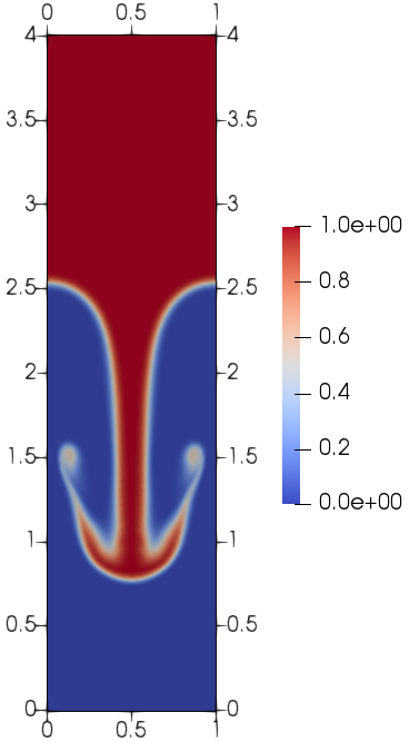
Figure 1: Rayleigh-Taylor instability, contour plot of the level set function at $t=T_{f}$.

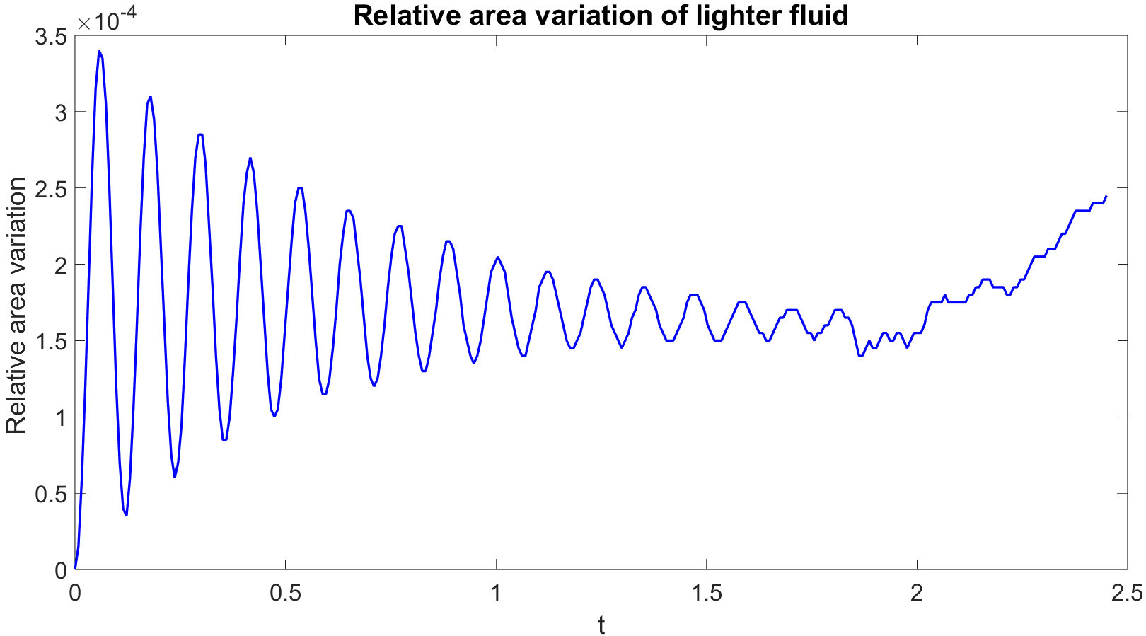
Figure 2: Rayleigh-Taylor instability, evolution of the relative variation of the area for the lighter fluid.

An interesting analysis regards the influence of the Atwood number. We fix $\rho_{2}=$0.408\text{\,}\mathrm{kg}\text{\,}{\mathrm{m}}^{-3}$$, so as to obtain $A\approx 0.5$. As a consequence, we obtain $t_{ref}\approx$0.451\text{\,}\mathrm{s}$,U_{ref}\approx$2.215\text{\,}\mathrm{m}\text{\,}{\mathrm{s}}^{-1}$,Re\approx 867.05,Fr\approx 0.71,$ and $M=0.006$. We set the final time $T_{f}=2$, so that the same final dimensional time of the previous configuration is achieved. The chosen time step is $\Delta t=2.5\cdot 10^{-3}$. One can easily notice from Figure 3 that, with higher Atwood number, the roll up effect is enhanced. This points out the earlier appearance of the Kelvin-Helmholtz instability, due to the development of short wavelength perturbations along the fluid interface.

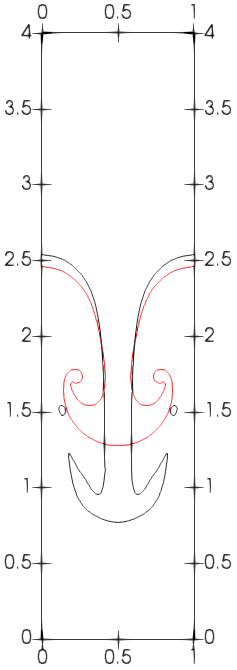
Figure 3: Rayleigh-Taylor instability, comparison between $A\approx 0.757$ and $A\approx 0.5$. The black line shows the interface for $A\approx 0.757$, whereas the red line refers to the interface for $A\approx 0.5$.

The deal.II library supports non-conforming mesh adaptation. We employ the $h$-adaptive version of the scheme for the latter configuration. More specifically, we define for each element $K$ the quantity

$$\eta_{K}=\max_{i\in\mathcal{N}_{K}}\left|\nabla\phi\right|_{i},$$ (95)

which acts as local refinement indicator. Here $\mathcal{N}_{K}$ denotes the set of nodes over the element $K$. We allow to refine when $\eta_{K}$ exceeds $10$ and to coarsen below $5$. The initial grid is composed by $80\times 320$ elements and we allow up to two local refinements, so as to obtain $h=\frac{1}{320}$ and a maximum resolution which would correspond to a $320\times 1280$ uniform grid. As one can notice from Figure 4, the refinement criterion is able to increase the resolution only in correspondence of the interface between the two fluids. The final grid consists of $43147$ elements, corresponding to around 40 % of elements of the fixed uniform grid. Figure 5 shows a comparison of the interface between the simulations with uniform and adaptive grid both at $t=\frac{T_{f}}{2}$ and $t=T_{f}$. One can easily notice that at $t=\frac{T_{f}}{2}$ the two interfaces are indistinguishable, whereas at $t=T_{f}$ a slightly different development of the instability appears. Since we are analyzing a fluid mechanic instability, every small variation in the flow corresponds to large variations, and, therefore, it is difficult to say which solution is the more reliable. Similar results and considerations have been reported for a Kelvin-Helmholtz instability in [36].

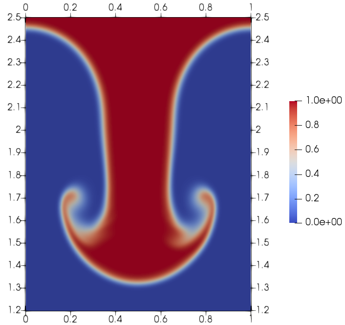
a)

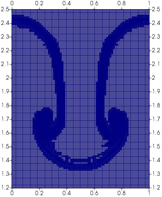
b)

Figure 4: Rayleigh-Taylor instability at $A\approx 0.5$, a) contour plot of the level set function at $t=T_{f}$, b) computational grid at $t=T_{f}$.

a)

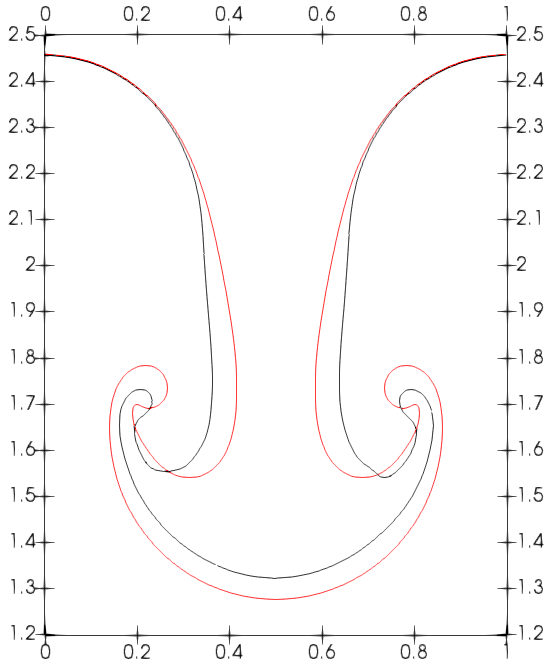
b)

Figure 5: Rayleigh-Taylor instability, comparison at $A\approx 0.5$ between the fixed grid simulation and the adaptive grid one: a) results at $t=\frac{T_{f}}{2}$, b) results at $t=T_{f}$. The black lines show the interface obtained with the adaptive grid, whereas the red lines refer to the interface obtained with the fixed grid.

5.2 Rising bubble benchmark

The rising bubble benchmark is a well-established test case for the validation of numerical methods for incompressible two-phase flows [27]. More specifically, the evolution of the shape, position and velocity of the center of mass of a rising bubble is compared against the reference solution in [27]. Two configurations are considered with the corresponding physical parameters and non-dimensional numbers listed in Table 1 and 2, respectively. The bubble occupies the subdomain $\Omega_{2}$. Following [27], we set $L_{ref}=2r_{0}=$0.5\text{\,}\mathrm{m}$$ and $U_{ref}=\sqrt{gL_{ref}}=$0.7\text{\,}\mathrm{m}\text{\,}{\mathrm{s}}^{-1}$$. We consider as domain $\Omega=\left(0,L_{x}\right)\times\left(0,L_{y}\right)$, with $L_{x}=2$ and $L_{y}=4$, whereas the final time is $T_{f}=4.2.$ No-slip boundary conditions are imposed on the top and bottom boundaries, whereas periodic conditions are prescribed in the horizontal direction. The initial velocity field is zero. Finally, the initial level set function is described by the following relation:

$$\phi(0)=\frac{1}{1+\exp\left(\frac{R-\sqrt{\left(x-x_{0}\right)^{2}+\left(y-y_{0}\right)^{2}}}{\varepsilon}\right)},$$ (96)

with $R=1,x_{0}=y_{0}=1$. We compute as reference quantities the position $\mathbf{x}_{c}$, the velocity $\mathbf{u}_{c}$ of the center of mass, and the so-called degree of circularity $\chi$, defined respectively as

$$\mathbf{x}_{c} = \frac{\int_{\Omega_{2}}\mathbf{x}d\Omega}{\int_{\Omega_{2}}d\Omega}=\frac{\int_{\Omega_{2}}\mathbf{x}d\Omega}{\left|\Omega_{2}\right|}$$ (97)

$$\mathbf{u}_{c} = \frac{\int_{\Omega_{2}}\mathbf{u}d\Omega}{\int_{\Omega_{2}}d\Omega}=\frac{\int_{\Omega_{2}}\mathbf{u}d\Omega}{\left|\Omega_{2}\right|}$$ (98)

$$\chi = \frac{2\sqrt{\pi\left|\Omega_{2}\right|}}{P_{b}},$$ (99)

where $\Omega_{2}$ is the subdomain occupied by the bubble, $\left|\Omega_{2}\right|$ is the area of the bubble, and $P_{b}$ is its perimeter. The degree of circularity is the ratio between the perimeter of a circle with the same area of the bubble and the current perimeter of the bubble itself. For a perfectly circular bubble, the degree of circularity is equal to one and then decreases as the bubble deforms itself. Since $\phi$ is a regularized Heaviside function, we can compute the reference quantities as follows:

$$\mathbf{x}_{c} \approx \frac{\int_{\Omega}\mathbf{x}\left(1-\phi\right)d\Omega}{\int_{\Omega}\left(1-\phi\right)d\Omega}$$ (100)

$$\mathbf{u}_{c} \approx \frac{\int_{\Omega}\mathbf{u}\left(1-\phi\right)d\Omega}{\int_{\Omega}\left(1-\phi\right)d\Omega}$$ (101)

$$\chi \approx \frac{2\sqrt{\pi\int_{\Omega}\left(1-\phi\right)d\Omega}}{\int_{\Omega}\left|\nabla\phi\right|d\Omega}.$$ (102)

Test case	$\rho_{1}\left[$\text{\,}\mathrm{kg}\text{\,}{\mathrm{m}}^{-3}$\right]$	$\rho_{2}\left[$\text{\,}\mathrm{kg}\text{\,}{\mathrm{m}}^{-3}$\right]$	$\mu_{1}\left[$\text{\,}\mathrm{kg}\text{\,}{\mathrm{m}}^{-1}\text{\,}{\mathrm{s}}^{-1}$\right]$	$\mu_{2}\left[$\text{\,}\mathrm{kg}\text{\,}{\mathrm{m}}^{-1}\text{\,}{\mathrm{s}}^{-1}$\right]$	$g\left[$\text{\,}\mathrm{m}\text{\,}{\mathrm{s}}^{-2}$\right]$	$\sigma\left[$\text{\,}\mathrm{kg}\text{\,}{\mathrm{s}}^{-2}$\right]$
Config. 1	$1000$	$100$	$10$	$1$	$0.98$	$24.5$
Config. 2	$1000$	$1$	$10$	$0.1$	$0.98$	$1.96$

Table 1: Physical parameters defining the configurations from rising bubble test case (data from [27].

Test case	$Re$	$Fr$	$We$	$\rho_{2}/\rho_{1}$	$\mu_{2}/\mu_{1}$
Config. 1	$35$	$1$	$10$	$10^{-1}$	$10^{-1}$
Config. 2	$35$	$1$	$125$	$10^{-3}$	$10^{-2}$

Table 2: Non-dimensional numbers defining the configurations from rising bubble test case (data from [27]).

We start with the first configuration and we set $M=0.0005$, corresponding to $c=$1400\text{\,}\mathrm{m}\text{\,}{\mathrm{s}}^{-1}$$, which is of the order of magnitude of the speed of sound in water. The computational grid is composed by $320\times 640$ elements, leading to $h=\frac{1}{160}$, whereas the time step is $\Delta t=6\cdot 10^{-3}$, yielding a maximum advective Courant number $C_{u}\approx 1.4$ and an acoustic Courant number $C=1920$. Finally, we set $\varepsilon=h,\Delta\tau=0.05h,u_{c}=0.05u_{max}$ and $\beta=0.5$. We point out here the fact that results in the Figures have been compared with the results of Group 2 in [27]. Figure 6 shows the shape of the bubble at $t=T_{f}$ and one can easily notice that we are able to recover the reference shape of the bubble. Figure 7 reports the evolution of the degree of circularity. A good qualitative agreement is established, with only slightly lower values for our numerical results. Figure 8 reports the evolution of the vertical coordinate of the position of the center of mass. For a quantitative point of view, the center of mass reaches $y_{c}=2.156$, which is in good agreement with the value $y_{c}=2.162\pm 0.002$ reported in [27]. Finally, Figure 9 shows the evolution of the vertical coordinate of the velocity of the center of mass. The maximum rise velocity of the center of mass is $v_{c}=0.3461$, which is again in good agreement with the value $v_{c}=0.3456\pm 0.0003$ present in [27].

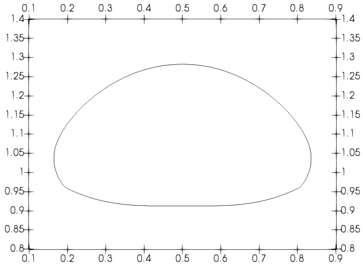
a)

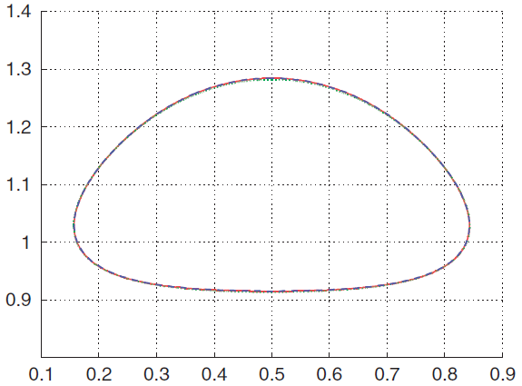
b)

Figure 6: Rising bubble benchmark, configuration 1, shape of bubble at $t=T_{f}$: a) numerical simulation, b) results from [27]. Bounds have been rescaled by $L_{ref}$ for the sake of comparison with reference results.

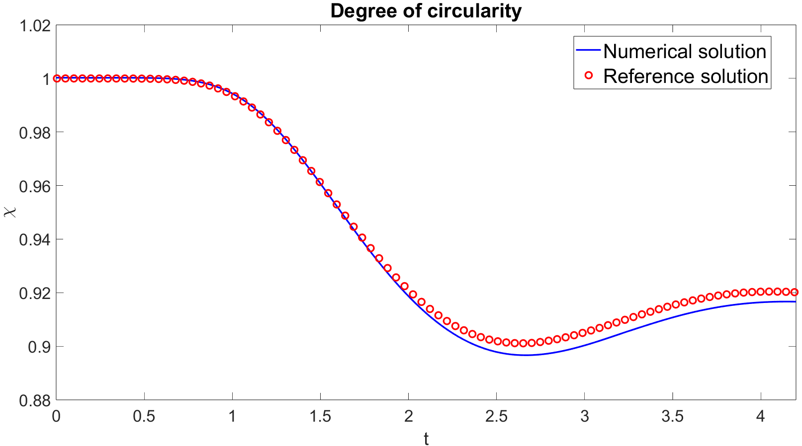
Figure 7: Rising bubble benchmark, configuration 1, degree of circularity. Reference results are from [27].

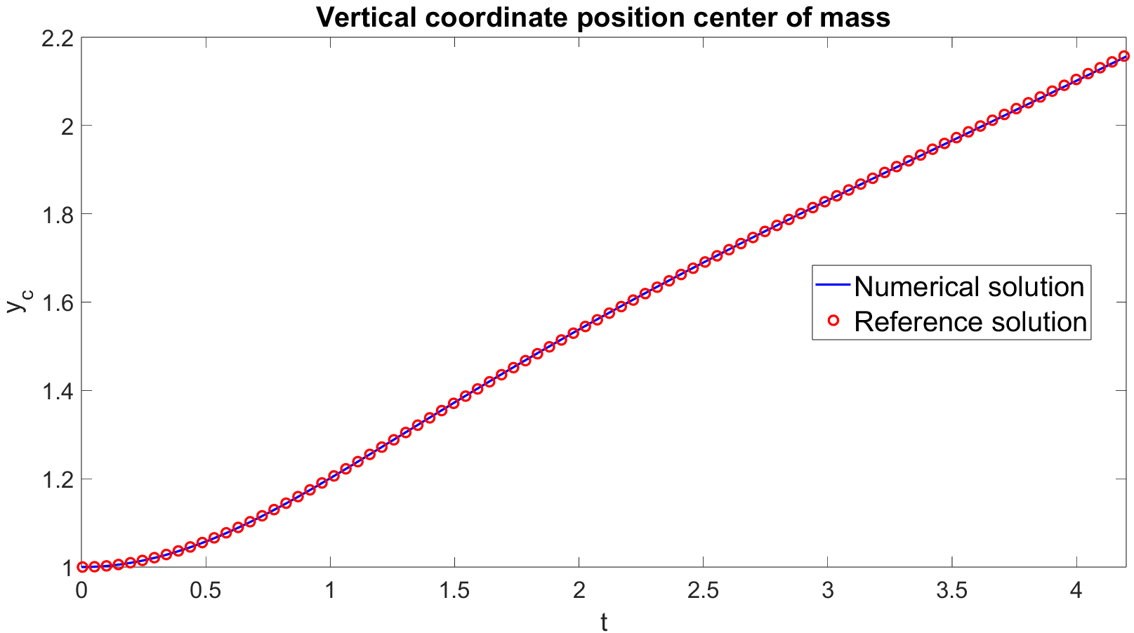
Figure 8: Rising bubble benchmark, configuration 1, vertical coordinate of the position of the center of mass. Reference results are from [27] and reference data have been multiplied by $L_{ref}$ for the sake of comparison.

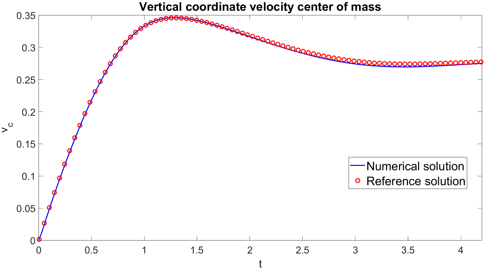
Figure 9: Rising bubble benchmark, configuration 1, vertical coordinate of the velocity of the center of mass. Reference results are from [27] and reference data have been multiplied by $U_{ref}$ for the sake of comparison.

We analyze now the second configuration. The time step is $\Delta t=5\cdot 10^{-3}$, yielding a maximum advective Courant number $C_{u}\approx 1.4$ and an acoustic Courant number $C=1600$. We also set $\varepsilon=h=\frac{1}{160},\Delta\tau=0.05h=3.125\times 10^{-4},u_{c}=0.0125u_{max}$ and $\beta=2$. Figure 10 shows the shape of the bubble at $t=T_{f}$. The bubble develops a non-convex shape with thin filaments. The solutions given in [27] are different and, in some cases, the thin filaments tend to break off, although it is unclear if such a phenomenon should be observed in the current two-dimensional setting. The obtained profile is however in good agreement with that of Group 2 in [27]. Figure 11, 12, 13 show the evolution of the degree of circularity, the vertical coordinate of the position of the center of mass, and the vertical coordinate of the velocity of the center of mass, respectively. A good qualitative agreement is established for the quantities of interest, even though deviations from the chosen reference solution are visible. In particular, differences appear for the degree of circularity starting from $t\approx 2.5$, when the thin filaments start developing. Moreover, the second peak for the rising velocity reaches a lower value. As mentioned above, there is no clear agreement concerning the thin filamentary regions, and, therefore, their development can strongly affect computations of the reference quantities and can lead to different numerical results.

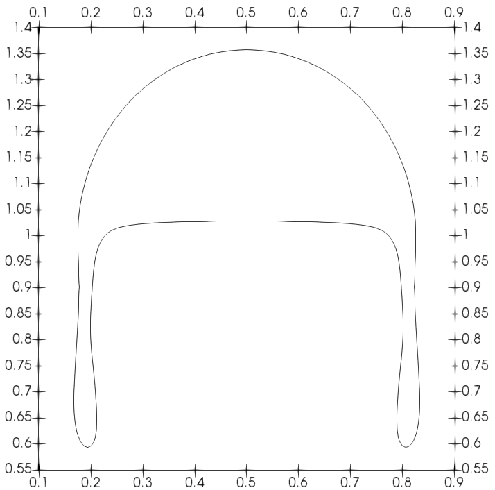
a)

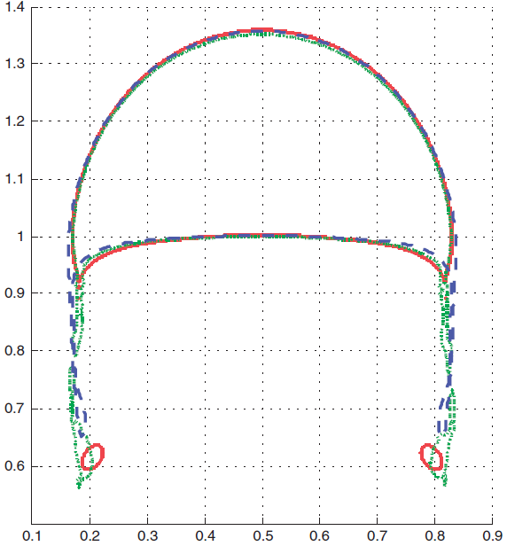
b)

Figure 10: Rising bubble benchmark, configuration 2, shape of bubble at $t=T_{f}$: a) numerical simulation, b) results from [27]. Bounds have been rescaled by $L_{ref}$ for the sake of comparison with the reference results.

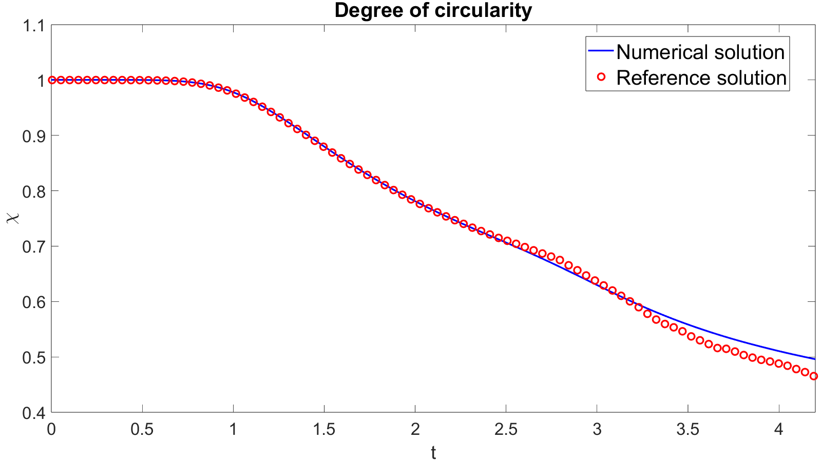
Figure 11: Rising bubble benchmark, configuration 2, degree of circularity. Reference results are from [27].

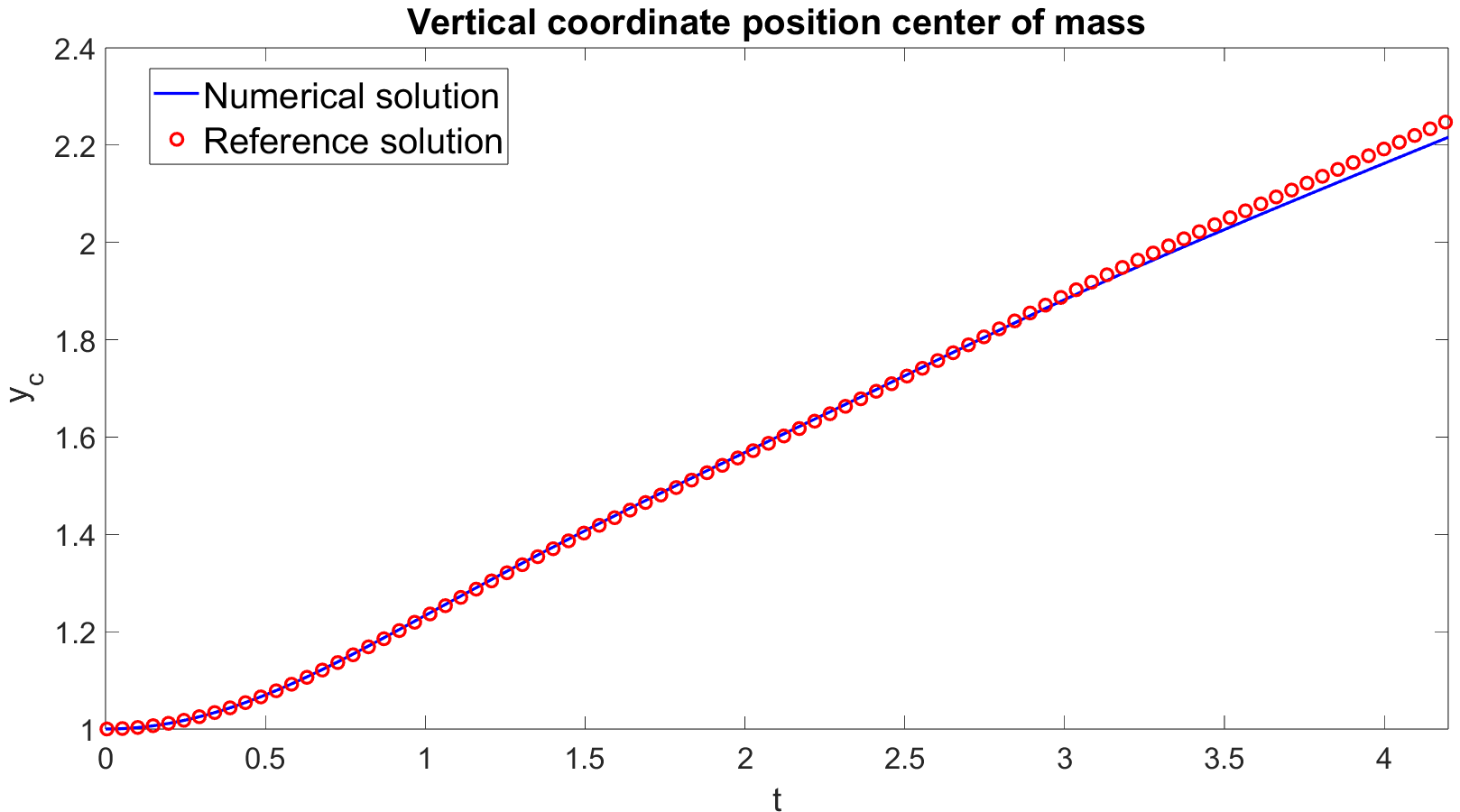
Figure 12: Rising bubble benchmark, configuration 2, vertical coordinate of the position of the center of mass. Reference results are from [27] and reference data have been multiplied by $L_{ref}$ for the sake of comparison.

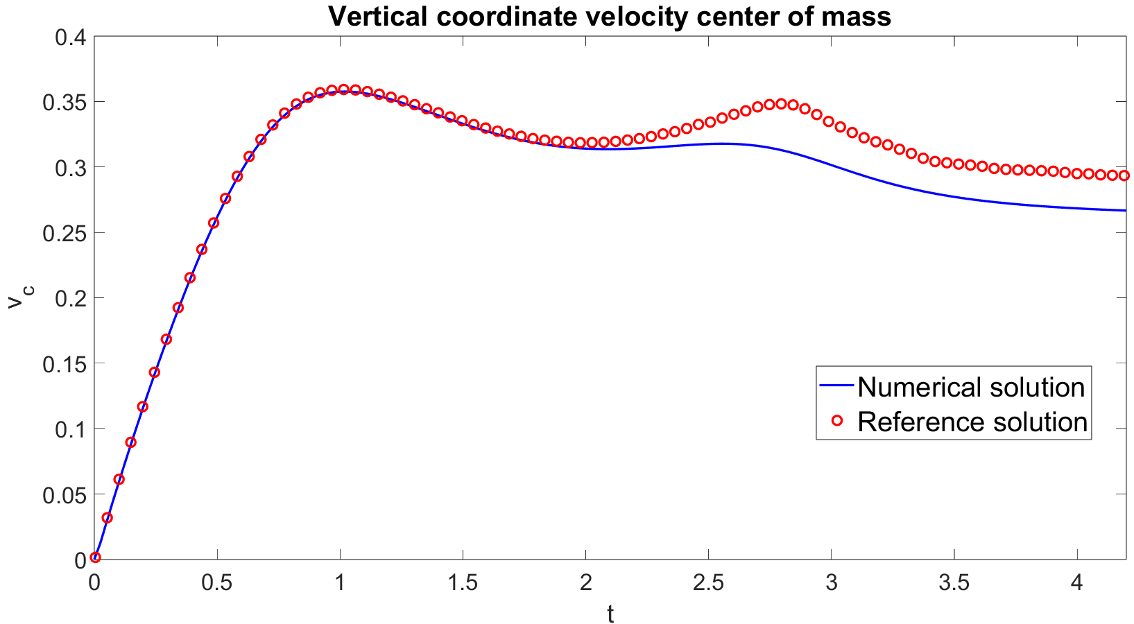
Figure 13: Rising bubble benchmark, configuration 2, vertical coordinate of the velocity of the center of mass. Reference results are from [27] and reference data have been multiplied by $U_{ref}$ for the sake of comparison.

We employ now Adaptive Mesh Refinement (AMR) to increase the resolution in correspondence of the interface. We consider the same refinement criterion (95) and the same thresholds for $\eta_{K}$ adopted in Section 5.1 and we allow up two local refinements, so as to obtain $h=\frac{1}{640}$ and a maximum resolution which would correspond to a $1280\times 2560$ uniform grid. Figure 14 shows both the shape of the bubble and the computational grid at $t=T_{f}$. One can notice that the resolution is enhanced close to the interface between the two fluids. The final grid consists of $283094$ elements. Figure 15 reports a comparison for the quantities of interest between the fixed grid simulation and the adaptive one. The results show that we have reached grid independence, since only the degree of circularity slightly differs between the two simulations, whereas the profiles of the vertical coordinates of both velocity and position of the center of mass are visually indistinguishable.

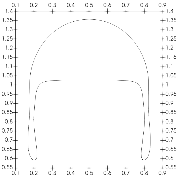
a)

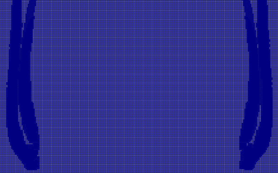
b)

Figure 14: Rising bubble benchmark, configuration 2 with adaptive mesh refinement, a) shape of bubble at $t=T_{f}$, b) computational grid at $t=T_{f}$ (close-up to thin filamentary regions).

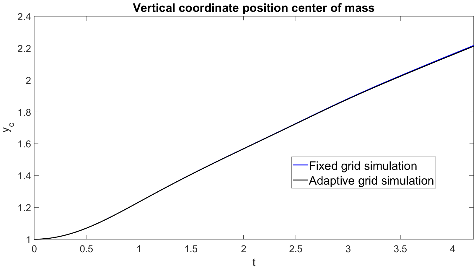
a)

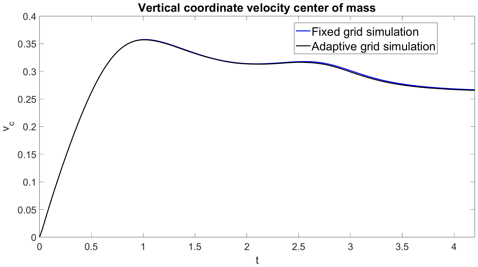
b)

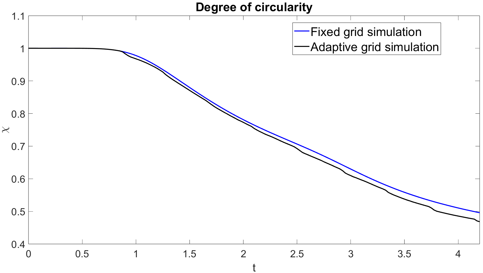
c)

Figure 15: Rising bubble benchmark, configuration 2 with adaptive mesh refinement, a) vertical coordinate position of the center of mass, b) vertical coordinate velocity of the center of mass, c) degree of circularity. The blue lines denote the results obtained with the uniform grid, whereas the black lines report the results obtained with the adaptive grid.

A significant difference in the development of the thin filamentary regions depends on the modelling of the viscosity coefficient $\mu$, as pointed out in [43] for diffuse interface models. A popular alternative to the linear interpolation model defined in (32) is the so-called harmonic interpolation, defined as

$$\frac{1}{\mu}=H_{\varepsilon}(\varphi)+\frac{\mu_{1}}{\mu_{2}}\left(1-H_{\varepsilon}(\varphi)\right).$$ (103)

This choice yields results which are more similar to Group 1 in [27], where a break-up occurs (see Figure 17). For what concerns the quantities of interest, we notice from Figure 17 that, since the thin elongated filaments break themselves, the degree of circularity is higher. Moreover, both the second peak of the rising velocity and the final position of the center of mass are significantly higher. The following analysis further confirms how challenging is defining a reference benchmark solution when the bubble undergoes large deformations.

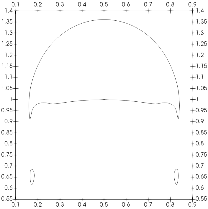
Figure 16: Rising bubble benchmark, configuration 2, shape of bubble at $t=T_{f}$ using the harmonic interpolation for the viscosity.

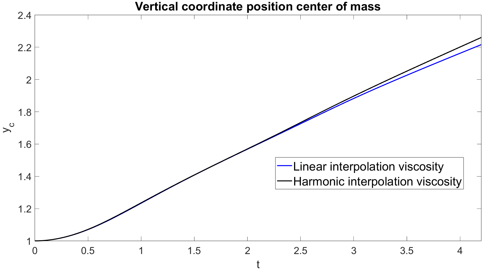
a)

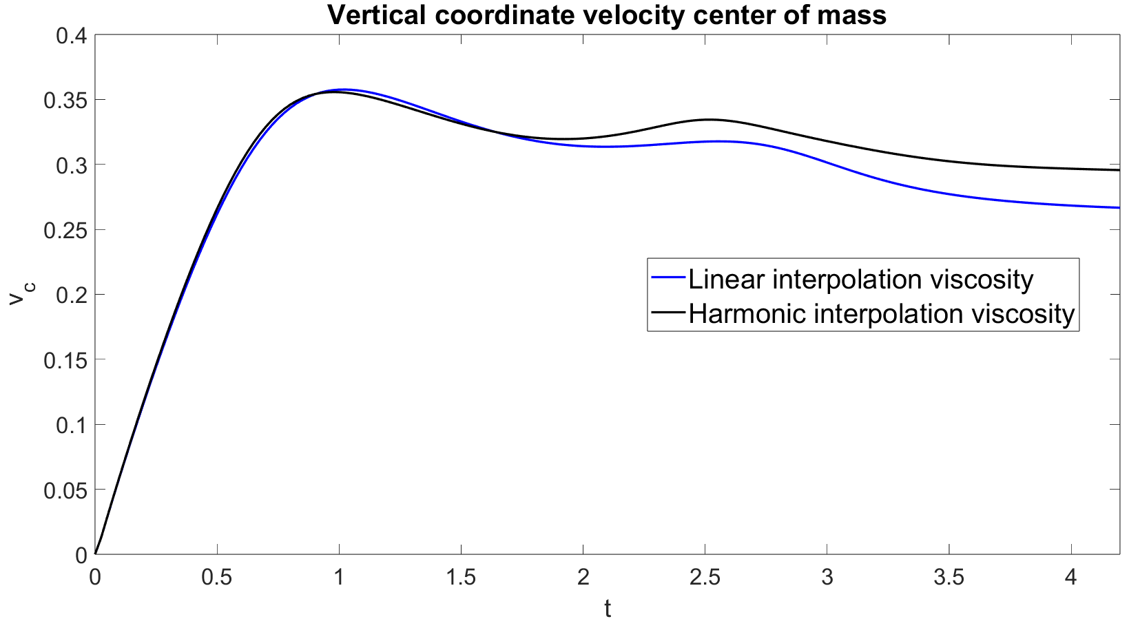
b)

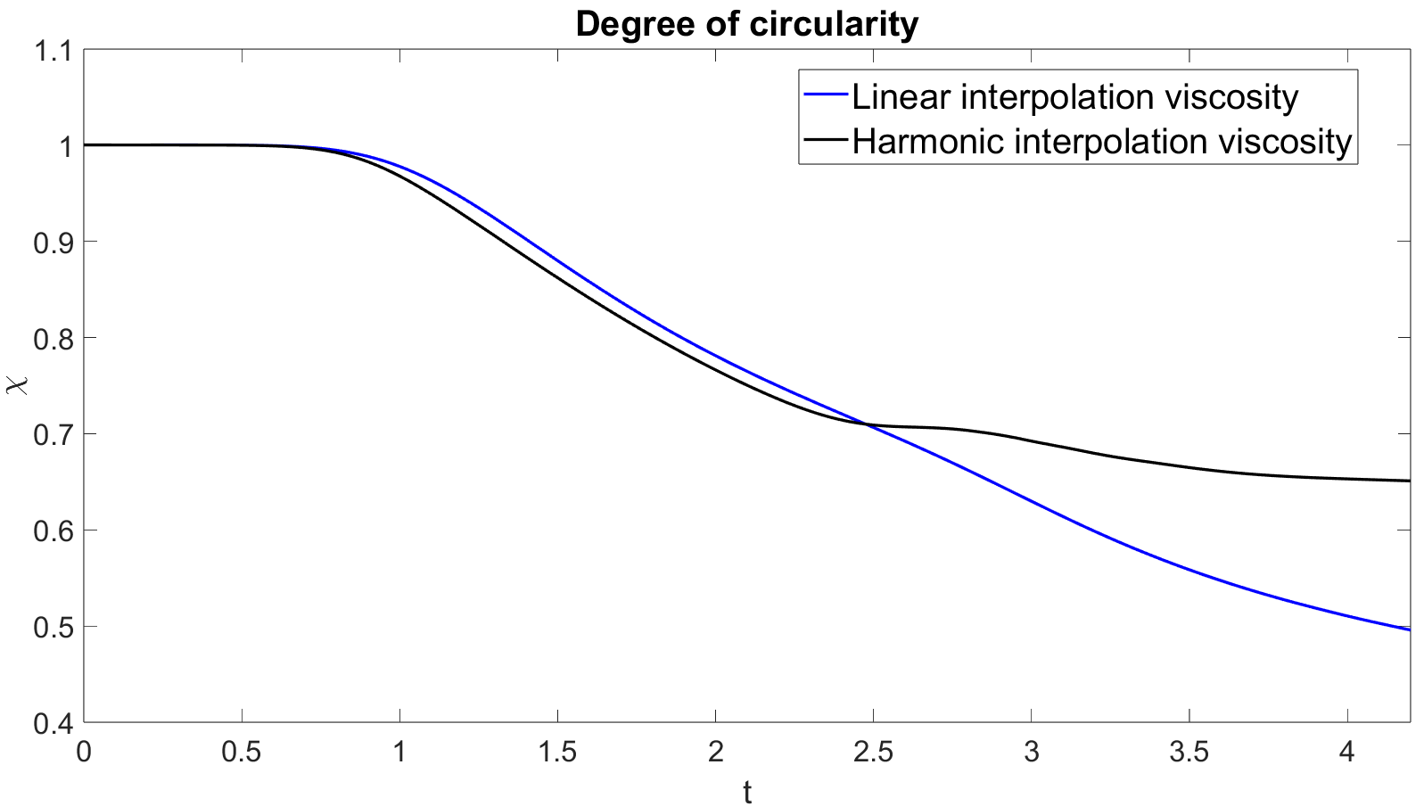
c)

Figure 17: Rising bubble benchmark, configuration 2, comparison between linear interpolation and harmonic interpolation for the viscosity: a) vertical coordinate of the position of the center of mass, b) vertical coordinate of the velocity of the center of mass, c) degree of circularity. The blue lines denote the results with the linear interpolation, whereas the black lines report the results with the harmonic interpolation.

6 Conclusions

Building on the experience of [35, 37], we have proposed an implicit Discontinuous Galerkin discretization for incompressible two-phase flows. While discretizations of incompressible two-phase flows equations have been proposed in many other papers, we have presented here an approach based on an artificial compressibility formulation in order to avoid some well known issues of projection methods. The time discretization is obtained by a projection method based on the L-stable TR-BDF2 method. The implementation has been carried out in the framework of the numerical library deal.II, whose mesh adaptation capabilities have been exploited to increase the resolution in correspondence of the interface between the two fluids. The effectiveness of the proposed approach has been shown in a number of classical benchmarks. In particular, for the rising bubble test case, the influence of some possible choices for the mixture viscosity when the interface undergoes large deformations has been established, following an analysis previously carried out for diffuse interface models. In future work, we aim to exploit the possibility of considering well resolved interfaces for an analysis on the evolution equations of interfacial quantities, as well as an extension of analogous approaches to fully compressible flows.

References

- [1] P.F. Antonietti, I. Mazzieri, A. Quarteroni, and F. Rapetti. Non-conforming high order approximations of the elastodynamics equation. Computer Methods in Applied Mechanics and Engineering, 209:212–238, 2012.
- [2] D. Arndt, W. Bangerth, M. Feder, M. Fehling, R. Gassmöller, T. Heister, L. Heltai, M. Kronbichler, M. Maier, P. Munch, J-P. Pelteret, S. Sticko, B. Turcksin, and D. Wells. The deal.II Library, Version 9.4. Journal of Numerical Mathematics, 0, 2022.
- [3] D.N. Arnold. An interior penalty finite element method with discontinuous elements. SIAM Journal of Numerical Analysis, 19:742–760, 1982.
- [4] R.E. Bank, W.M. Coughran, W. Fichtner, E.H. Grosse, D.J. Rose, and R.K. Smith. Transient simulation of silicon devices and circuits. IEEE Transactions on Computer-Aided Design of Integrated Circuits and Systems, 4(4):436–451, 1985.
- [5] C. Bassi, A. Abbà, L. Bonaventura, and L. Valdettaro. Large eddy simulation of non-Boussinesq gravity currents with a DG method. Theoretical and Computational Fluid Dynamics, 34:231–247, 2020.
- [6] F. Bassi, L.A. Botti, A. Colombo, and F.C. Massa. Assessment of an Implicit Discontinuous Galerkin Solver for Incompressible Flow Problems with Variable Density. Applied Sciences, 12(21):11229, 2022.
- [7] F. Bassi, A. Crivellini, D.A. Di Pietro, and S. Rebay. An artificial compressibility flux for the discontinuous Galerkin solution of the incompressible Navier-Stokes equations. Journal of Computational Physics, 218:794–815, 2006.
- [8] F. Bassi and S. Rebay. A high-order accurate discontinuous finite element method for the numerical solution of the compressible Navier-Stokes equations. Journal of Computational Physics, 131(2):267–279, 1997.
- [9] L. Bonaventura and A. Della Rocca. Unconditionally strong stability preserving extensions of the TR-BDF2 method. Journal of Scientific Computing, 70:859–895, 2017.
- [10] J.U. Brackbill, D.B. Kothe, and C. Zemach. A continuum method for modeling surface tension. Journal of Computational Physics, 100(2):335–354, 1992.
- [11] P.H. Chiu and Y.T. Lin. A conservative phase field method for solving incompressible two-phase flows. Journal of Computational Physics, 230(1):185–204, 2011.
- [12] A.J. Chorin. A numerical method for solving incompressible viscous flow problems. Journal of Computational Physics, 2:12–26, 1967.
- [13] A.J. Chorin. Numerical solution of the Navier-Stokes equations. Mathematics of computation, 22(104):745–762, 1968.
- [14] A. Della Rocca. Large-Eddy Simulations of Turbulent Reacting Flows with Industrial Applications. PhD thesis, Politecnico di Milano, 2 2018.
- [15] W. Dettmer, P.H. Saksono, and D. Perić. On a finite element formulation for incompressible Newtonian fluid flows on moving domains in the presence of surface tension. Communications in Numerical Methods in Engineering, 19(9):659–668, 2003.
- [16] D.A. Di Pietro, S. Lo Forte, and N. Parolini. Mass preserving finite element implementations of the level set method. Applied Numerical Mathematics, 56(9):1179–1195, 2006.
- [17] R. Estrada and R.P. Kanwal. Applications of distributional derivatives to wave propagation. IMA Journal of Applied Mathematics, 26(1):39–63, 1980.
- [18] R. Fedkin and S. Osher. The Level Set Methods and Dynamic Implicit Surfaces. Springer Nature, 2003.
- [19] N. Fehn, M. Kronbichler, C. Lehrenfeld, G. Lube, and P. Schroeder. High-order DG solvers for under-resolved turbulent incompressible flows: A comparison of and methods. International Journal of Numerical Methods in Fluids, 91:533–556, 2019.
- [20] N. Fehn, W.A. Wall, and M. Kronbichler. On the stability of projection methods for the incompressible Navier-Stokes equations based on high-order discontinuous Galerkin discretizations. Journal of Computational Physics, 351:392–421, 2017.
- [21] P. Gao, J. Ouyang, and W. Zhou. Development of a finite element/discontinuous Galerkin/level set approach for the simulation of incompressible two phase flow. Advances in Engineering Software, 118:45–59, 2018.
- [22] J. Grooss and J.S. Hesthaven. A level set discontinuous Galerkin method for free surface flows. Computer Methods in Applied Mechanics and Engineering, 195(25-28):3406–3429, 2006.
- [23] J.L. Guermond, P. Minev, and J. Shen. An overview of projection methods for incompressible flows. Computer Methods in Applied Mechanics and Engineering, 195(44-47):6011–6045, 2006.
- [24] M. Haghshenas, J.A. Wilson, and R. Kumar. Algebraic coupled level set-volume of fluid method for surface tension dominant two-phase flows. International Journal of Multiphase Flow, 90:13–28, 2017.
- [25] M.E. Hosea and L.F. Shampine. Analysis and implementation of TR-BDF2. Applied Numerical Mathematics, 20(1-2):21–37, 1996.
- [26] T.J.R. Hughes, W.K. Liu, and T.K. Zimmermann. Lagrangian-Eulerian finite element formulation for incompressible viscous flows. Computer Methods in Applied Mechanics and Engineering, 29(3):329–349, 1981.
- [27] S. Hysing, S. Turek, D. Kuzmin, N. Parolini, E. Burman, S. Ganesan, and L. Tobiska. Quantitative benchmark computations of two-dimensional bubble dynamics. International Journal for Numerical Methods in Fluids, 60(11):1259–1288, 2009.
- [28] G. Karniadakis and S. Sherwin. Spectral/hp element methods for computational fluid dynamics. Oxford University Press on Demand, 2005.
- [29] M. Kronbichler, A. Diagne, and H. Holmgren. A fast massively parallel two-phase flow solver for microfluidic chip simulation. The International Journal of High Performance Computing Applications, 32(2):266–287, 2018.
- [30] B. Lafaurie, C. Nardone, R. Scardovelli, S. Zaleski, and G. Zanetti. Modelling merging and fragmentation in multiphase flows with surfer. Journal of Computational Physics, 113(1):134–147, 1994.
- [31] Juan Manzanero, Gonzalo Rubio, David A Kopriva, Esteban Ferrer, and Eusebio Valero. An entropy-stable discontinuous Galerkin approximation for the incompressible Navier-Stokes equations with variable density and artificial compressibility. Journal of Computational Physics, 408:109241, 2020.
- [32] S. Mirjalili, S.S. Jain, and M. Dodd. Interface-capturing methods for two-phase flows: An overview and recent developments. Center for Turbulence Research Annual Research Briefs, 2017(117-135):13, 2017.
- [33] E. Olsson and G. Kreiss. A conservative level set method for two phase flow. Journal of Computational Physics, 210(1):225–246, 2005.
- [34] E. Olsson, G. Kreiss, and S. Zahedi. A conservative level set method for two phase flow ii. Journal of Computational Physics, 225(1):785–807, 2007.
- [35] G. Orlando. Modelling and simulations of two-phase flows including geometric variables. PhD thesis, Politecnico di Milano, 2023. http://hdl.handle.net/10589/198599.
- [36] G. Orlando, T. Benacchio, and L. Bonaventura. An IMEX-DG solver for atmospheric dynamics simulations with adaptive mesh refinement. Journal of Computational and Applied Mathematics, 427:115124, 2023.
- [37] G. Orlando, A. Della Rocca, P.F. Barbante, L. Bonaventura, and N. Parolini. An efficient and accurate implicit DG solver for the incompressible Navier-Stokes equations. International Journal for Numerical Methods in Fluids, 94(9):1484–1516, 2022.
- [38] S. Osher and R.P. Fedkiw. Level set methods and dynamic implicit surfaces, volume 1. Springer New York, 2005.
- [39] S. Osher and J.A. Sethian. Fronts propagating with curvature-dependent speed: Algorithms based on Hamilton-Jacobi formulations. Journal of Computational Physics, 79(1):12–49, 1988.
- [40] M. Owkes and O. Desjardins. A discontinuous Galerkin conservative level set scheme for interface capturing in multiphase flows. Journal of Computational Physics, 249:275–302, 2013.
- [41] F. Pochet, K. Hillewaert, P. Geuzaine, J.F. Remacle, and E. Marchandise. A 3d strongly coupled implicit discontinuous Galerkin level set-based method for modeling two-phase flows. Computers & Fluids, 87:144–155, 2013.
- [42] S. Popinet and S. Zaleski. A front-tracking algorithm for accurate representation of surface tension. International Journal for Numerical Methods in Fluids, 30(6):775–793, 1999.
- [43] M. Řehoř. Diffuse interface models in theory of interacting continua. PhD thesis, 2018.
- [44] M. Rudman. Volume-tracking methods for interfacial flow calculations. International Journal for Numerical Methods in Fluids, 24(7):671–691, 1997.
- [45] H. Rusche. Computational fluid dynamics of dispersed two-phase flows at high phase fractions. PhD thesis, Imperial College London (University of London), 2003.
- [46] S. Salsa. Partial differential equations in action: from modelling to theory, volume 99. Springer, 2016.
- [47] D. Schötzau, C. Schwab, and A. Toselli. Stabilized DGFEM for incompressible flows. Mathematical Models and Methods in Applied Sciences, 13:1413–1436, 2003.
- [48] T.W.H. Sheu, C.H. Yu, and P.H. Chiu. Development of a dispersively accurate conservative level set scheme for capturing interface in two-phase flows. Journal of Computational Physics, 228(3):661–686, 2009.
- [49] M. Sussman, P. Smereka, and S. Osher. A level set approach for computing solutions to incompressible two-phase flow. Journal of Computational physics, 114(1):146–159, 1994.
- [50] R. Temam. Sur l’approximation de la solution des équations de Navier-Stokes par la méthode des pas fractionnaires (ii). Archive for rational mechanics and analysis, 33:377–385, 1969.
- [51] A. Toselli. Discontinuous Galerkin approximations for the Stokes problem. Mathematical Models and Methods in Applied Sciences, 12:1565–1597, 2002.
- [52] G. Tryggvason. Numerical simulations of the rayleigh-taylor instability. Journal of Computational Physics, 75(2):253–282, 1988.
- [53] S. Zahedi. Numerical methods for fluid interface problems. PhD thesis, KTH Royal Institute of Technology, 2011.