Alleviating Matthew Effect of Offline Reinforcement Learning
in Interactive Recommendation

Abstract.

Offline reinforcement learning (RL), a technology that offline learns a policy from logged data without the need to interact with online environments, has become a favorable choice in decision-making processes like interactive recommendation. Offline RL faces the value overestimation problem. To address it, existing methods employ conservatism, e.g., by constraining the learned policy to be close to behavior policies or punishing the rarely visited state-action pairs. However, when applying such offline RL to recommendation, it will cause a severe Matthew effect, i.e., the rich get richer and the poor get poorer, by promoting popular items or categories while suppressing the less popular ones. It is a notorious issue that needs to be addressed in practical recommender systems.

In this paper, we aim to alleviate the Matthew effect in offline RL-based recommendation. Through theoretical analyses, we find that the conservatism of existing methods fails in pursuing users’ long-term satisfaction. It inspires us to add a penalty term to relax the pessimism on states with high entropy of the logging policy and indirectly penalizes actions leading to less diverse states. This leads to the main technical contribution of the work: Debiased model-based Offline RL (DORL) method. Experiments show that DORL not only captures user interests well but also alleviates the Matthew effect. The implementation is available via https://github.com/chongminggao/DORL-codes.

1. Introduction

Recommender systems, a powerful tool for helping users select preferred items from massive items, are continuously investigated by e-commerce companies. Previously, researchers tried to dig up static user interests from historical data by developing supervised learning-based recommender models. With the recent development of deep learning and the rapid growth of available data, fitting user interests is not a bottleneck for now.

A desired recommendation policy should be able to satisfy users for a long time (Wang et al., 2022b). Therefore, it is natural to involve Reinforcement Learning (RL) which is a type of Machine Learning concerned with how an intelligent agent can take actions to pursue a long-term goal (Afsar et al., 2022; Cai et al., 2023a; Liu et al., 2023; Cai et al., 2023b). In this setting, the recommendation process is formulated as a sequential decision process where the recommender interacts with users and receives users’ online feedback (i.e., rewards) to optimize users’ long-term engagement, rather than fitting a model on a set of samples based on supervised learning (Chen et al., 2022; Zou et al., 2019; Xue et al., 2023). However, it is expensive and impractical to learn a policy from scratch with real users, which becomes the main obstacle that impedes the deployment of RL to recommender systems.

One remedy is to leverage historical interaction sequences, i.e., recommendation logs, to conduct offline RL (also called batch RL) (Levine et al., 2020). The objective is to learn an online policy that makes counterfactual decisions to perform better than the behavior policies induced by the offline data. However, without real-time feedback, directly employing conventional online RL algorithms in offline scenarios will result in poor performance due to the value overestimation problem in offline RL. The problem is induced when the function approximator of the agent tries to extrapolate values (e.g., Q-values in Q-learning (Watkins and Dayan, 1992)) for the state-action pairs that are not well-covered by logged data. More specifically, since the RL model usually maximizes the expected value or trajectory reward, it will intrinsically prefer overestimated values induced by the extrapolation error, and the error will be compounded in the bootstrapping process when estimating Q-values, which results in unstable learning and divergence (Kumar et al., 2019). In recommendation, this may lead to an overestimation of user preferences for items that infrequently appear in the offline logs.

This is the core challenge for offline RL algorithms because of the inevitable mismatch between the offline dataset and the learned policy (Wang et al., 2020a). To solve this problem, offline RL algorithms incorporate conservatism into the policy design. Model-free offline RL algorithms directly incorporate conservatism by constraining the learned policy to be close to the behavior policy (Fujimoto et al., 2019b; Kumar et al., 2019), or by penalizing the learned value functions from being over-optimistic upon out-of-distribution (OOD) decisions (Kumar et al., 2020). Model-based offline RL algorithms learn a pessimistic model as a proxy of the environment, which results in a conservative policy (Kidambi et al., 2020; Yu et al., 2020). This philosophy guarantees that offline RL models can stick to offline data without making OOD actions, which has been proven to be effective in lots of domains, such as robotic control (Ebert et al., 2018) or games (Agarwal et al., 2020).

However, applying conservatism to recommender systems gives rise to a severe Matthew effect (Liu and Huang, 2021), which can be summarized as “the rich get richer and the poor get poorer”. In recommendation, it means that the popular items or categories in previous data will get larger opportunities to be recommended later, whereas the unpopular ones get neglected. This is catastrophic since users desire diverse recommendations and the repetition of certain contents will incur the filter bubble issue, which in turn hurts users’ satisfaction even though users favored them before (Gao et al., 2022a, d; Tomlein et al., 2021; Zhang et al., 2023). We will show the Matthew effect in the existing offline RL-based recommender (Fig. 3), and analyze how users’ satisfaction will be hurt (Fig. 2).

In this paper, we embrace the model-based RL paradigm. The basic idea is to learn a user model (i.e., world model) that captures users’ preferences, then use it as a pseudo-environment (i.e., simulated users) to produce rewards to train a recommendation policy. Compared to model-free RL, model-based RL has several advantages in recommendation. First and foremost, model-based RL is much more sample efficient (Yu et al., 2020). That it needs significantly fewer samples makes it more suitable for the highly sparse recommendation data. Second, explicitly learning the user model simplifies the problem and makes it easier to incorporate expert knowledge. For example, the user model can be implemented as any state-of-the-art recommendation model (e.g., DeepFM (Guo et al., 2017) in this work) or sophisticated generative adversarial frameworks (Xue et al., 2023; Zhao et al., 2021). Although some works have adopted this paradigm in their recommender systems (Gao et al., 2022a; Huang et al., 2022, 2020; Zou et al., 2020), they did not explicitly consider the value overestimation problem in offline RL, not to mention the Matthew effect in the solutions.

To address the value overestimation problem while reducing the Matthew effect, we propose a Debiased model-based Offline RL (DORL) method for recommendation. By theoretically analyzing the mismatch between real users’ long-term satisfaction and the preferences estimated from the offline data, DORL adds a penalty term that relaxes the pessimism on states with high entropy of the logging policy and indirectly penalizes actions leading to less diverse states. By introducing such a counterfactual exploration mechanism, DORL can alleviate the Matthew effect in final recommendations. Our contributions are summarized as:

• We point out that conservatism in offline RL can incur the Matthew effect in recommendation. We show this phenomenon in existing methods and how it hurts user satisfaction.

• After theoretically analyzing how existing methods fail in recommendation, we propose the DORL model that introduces a counterfactual exploration in offline data.

• We demonstrate the effectiveness of DORL in an interactive recommendation setting, where alleviating the Matthew effect increases users’ long-term experience.

2. Related Work

Here, we briefly review the Matthew effect in recommendation. We introduce the interactive recommendation and offline RL.

2.1. Matthew Effect in Recommendation

Liu and Huang (2021) confirmed the existence of the Matthew effect in YouTube’s recommendation system, and Wang et al. (2018) gave a quantitative analysis of the Matthew effect in collaborative filtering-based recommenders. A common way of mitigating the Matthew effect in recommendation is to take into account diversity (Anderson et al., 2020; Zheng et al., 2021a; Liang et al., 2021; Hansen et al., 2021). Another perspective on this problem is to remove popularity bias (Zheng et al., 2021b). We consider the Matthew effect in offline RL-based recommendation systems. we will analyze why this problem occurs and provide a novel way to address it.

2.2. Interactive Recommendation

The interactive recommendation is a setting where a model interacts with a user online (Wu et al., 2022; Gao et al., 2021; Lei et al., 2021). The model recommends items to the user and receives the user’s real-time feedback. This process is repeated until the user quits. The model will update its policy with the goal to maximize the cumulative satisfaction over the whole interaction process (instead of learning on I.I.D. samples). This setting well reflects the real-world recommendation scenarios, for example, a user will continuously watch short videos and leave feedback (e.g. click, add to favorite) until he chooses to quit.

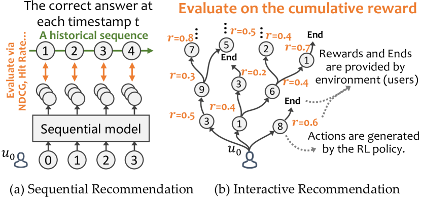
Figure 1. Illustration of evaluations in the traditional sequential recommendation and interactive recommendation settings.

Here, we emphasize the most notable difference between the interactive recommendation setting and traditional sequential recommendation settings (Xin et al., 2022, 2020). Fig. 1 illustrates the learning and evaluation processes in sequential and interactive recommendation settings. Sequential recommendation uses the philosophy of supervised learning, i.e., evaluating the top-$k$ results by comparing them with a set of “correct” answers in the test set and computing metrics such as Precision, Recall, NDCG, and Hit Rate. By contrast, interactive recommendation evaluates the results by accumulating the rewards along the interaction trajectories. There is no standard answer in interactive recommendation, which is challenging (Deffayet et al., 2023).

Interactive recommendation requires offline data of high quality, which hampers the development of this field for a long time. We overcome this problem by using the recently-proposed datasets that support interactive learning and off-policy evaluation (Gilotte et al., 2018).

2.3. Offline Reinforcement Learning

Recently, many offline RL models have been proposed to overcome the value overestimation problem. For model-free methods, BCQ (Fujimoto et al., 2019b) uses a generative model to constrain probabilities of state-action pairs the policy utilizes, thus avoiding using rarely visited data to update the value network; CQL (Kumar et al., 2020) contains a conservative strategy to penalize the overestimated Q-values for the state-action pairs that have not appeared in the offline data; GAIL (Ho and Ermon, 2016) utilizes a discriminator network to distinguish between expert policies with others for imitation learning. IQL (Kostrikov et al., 2022) enables the learned policy to improve substantially over the best behavior in the data through generalization, without ever directly querying a Q-function with unseen actions. For model-based methods, MOPO (Yu et al., 2020) learns a pessimistic dynamics model and use it to learn a conservative estimate of the value function; COMBO (Yu et al., 2021) learns the value function based on both the offline dataset and data generated via model rollouts, and it suppresses the value function on OOD data generated by the model. Almost all offline RL methods have a similar philosophy: to introduce conservatism or pessimism in the learned policy (Levine et al., 2020).

There are efforts to conduct offline RL in recommendation (Xiao and Wang, 2021; Gao et al., 2022a; Huang et al., 2020; Jeunen and Goethals, 2021; Chen et al., 2019). However, few works explicitly discuss the Matthew effect in recommendation. Chen et al. (2019) mentioned this effect in their experiment section, but their method is not tailored to overcome this issue.

3. Empirical Study on Matthew Effect

We conduct empirical studies in recommendation to show how the Matthew effect affects user satisfaction. When the Matthew effect is amplified, the recommender will repeatedly recommend the items with dominant categories. To illustrate the long-term effect on user experience, we explore the logs of the KuaiRand-27K video dataset (Gao et al., 2022c) and the LFM-1b music dataset (Schedl, 2016). KuaiRand-27K contains a 23 GB log recording 27,285 users’ 322,278,385 interactions on 32,038,725 videos with 62 categories, which are collected from April 8th, 2022 to May 8th, 2022. LFM-1b contains a 40GB log recording 120,322 users’ 1,088,161,692 listening events on 32,291,134 tracks with 3,190,371 artists, which are fetched from Last.FM in the range from January 2013 to August 2014.

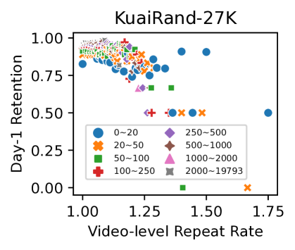
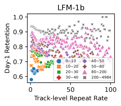
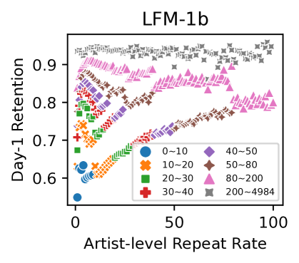
Figure 2. An increase in the repeat rate (i.e., the Matthew effect) negatively impacts user experience. In nearly all activity level groups marked by different colors and maker types, Day-1 Retention of users declines as the repeat rate rises.

Both the two datasets provide the timestamp of each event, hence we can assess the long-term effect of overexposure by investigating the change of Day-1 Retention. Day-1 Retention is defined as the probability of a user who returns to the app tomorrow after finishing today’s viewing/listening. This metric is more convincing than real-time signals (e.g., click, adding to favorite) in regard to reflecting the long-term effect on user satisfaction. We consider the item-level and category/artist-level repeat rates as the metrics to measure the Matthew effect. The item-level (or category-level) repeat rate of a user viewing videos on a certain day is defined as:

$$\frac{\text{the number of viewing events}}{\text{the number of unique videos (or unique categories)}}.$$

For example, if a user views 5 unique videos (which belong to 3 unique categories) 20 times in a day, then the item-level repeat rate is 20/5=4.0 and the category-level repeat rate is 20/3=6.67. The item-level and artist-level repeat rates for music listening are defined in a similar way. Note that in KuaiRand, video-level overexposure rarely appears because of the rule of video recommendation, i.e., the same video will not be recommended twice.

In this definition, user activity can become a confounder. For instance, a user who views 100 videos a day can be more active than a user who views only 10 videos a day, and thus is more likely to revisit the App the next day. Therefore, we control for this confounder by splitting the users w.r.t. the number of their daily viewing events. Groups with different user activity levels are marked by different colors and marker types. The results are shown in Fig. 2.

In short, Day-1 Retention reduces when the repeat rate increases in each group with a user activity level. This phenomenon can be observed for both the item-level and category/artist-level repeat rates within the video dataset and music dataset. The results show that users’ satisfaction will be hurt when the Matthew effect becomes severer.

4. Preliminary on Model-based RL

We introduce the basics of RL and model-based offline RL.

4.1. Basics of Reinforcement Learning

Reinforcement learning (RL) is the science of decision making. We usually formulate the problem as a Markov decision process (MDP): $M=(\mathcal{S},\mathcal{A},T,r,\gamma)$, where $\mathcal{S}$ and $\mathcal{A}$ represent the state space and action space, $T(s,a,s^{\prime})=P(s_{t+1}=s^{\prime}|s_{t}=s,a_{t}=a)$ is the transition probability from $(s,a)$ to $s^{\prime}$, $r(s,a)$ is the reward of taking action $a$ at state $s$, and $\gamma$ is the discount factor. Accordingly, the offline MDP can be denoted as $\widehat{M}=(\mathcal{S},\mathcal{A},\widehat{T},\hat{r},\gamma)$, where $\widehat{T}$ and $\hat{r}$ are the transition probability and reward function predicted by an offline model. In offline RL, the policy is trained on an offline dataset $\mathcal{D}$ which was collected by a behavior policy $\pi_{\beta}$ running in online environment $M$. By modifying the offline MDP $\widehat{M}$ to be conservative for overcoming the value overestimation issue, we will derive a modified MDP $\widetilde{M}=(\mathcal{S},\mathcal{A},\widehat{T},\widetilde{r},\gamma)$, where the modified reward $\widetilde{r}$ is modified from the predicted reward $\hat{r}$.

Since RL considers long-term utility, we can define the value function as $V_{M}^{\pi}(s)=\mathbb{E}_{\pi,T}[\sum_{t=0}^{\infty}\gamma^{t}r(s_{t},a_{t})|s_{0}=s]$, denoting the cumulative reward gain by policy $\pi$ after state $s$ in MDP $M$. Let $P_{T,t}^{\pi}$ be the probability of the agent’s being in state $s$ at time $t$, if the agent uses policy $\pi$ and transits with $T$. Defining $\rho_{T}^{\pi}(s,a)=(1-\gamma)\pi(a|s)\sum_{t=0}^{\infty}\gamma^{t}P_{T,t}^{\pi}(s)$ as the discounted distribution of state-action pair $(s,a)$ for policy $\pi$ over $T$, we can derive another form of the policy’s accumulated reward as $\eta_{M}(\pi)=\mathbb{E}_{(s,a)\sim\rho_{T}^{\pi}}[r(s,a)]$.

4.2. Model-Based Offline RL Framework

In this paper, we follow a state-of-the-art general Model-based Offline Policy Optimization framework, MOPO (Yu et al., 2020). The basic idea is to learn a dynamics model $\widehat{T}$ which captures the state transition $(s,a)\rightarrow s^{\prime}$ of the environment and estimates reward $\hat{r}(s,a)$ given state $s$ and action $a$. For addressing the distributional shift problem where values $V_{\widehat{M}}^{\pi}(s)$ are usually over-optimistically estimated, MOPO introduces a penalty function $p(s,a)$ on the estimated reward $\hat{r}(s,a)$ as:

(1) $$\tilde{r}(s,a)=\hat{r}(s,a)-\lambda p(s,a).$$

On the modified reward $\tilde{r}(s,a)$, the offline MDP $\widehat{M}$ will be modified to be a conservative MDP: $\widetilde{M}=(\mathcal{S},\mathcal{A},\widehat{T},\tilde{r},\gamma)$. MOPO learns its policy in this MDP: $\widetilde{M}$. By defining $\epsilon_{p}(\pi)=\mathbb{E}_{(s,a)\sim\rho_{\widehat{T}}^{\pi}}[p(s,a)]$, MOPO has the following theoretical guarantee:

Theorem 4.1.

If the penalizer $p(s,a)$ meets:

(2) $$\lambda\mathbb{E}_{(s,a)\sim\rho_{\widehat{T}}^{\pi}}[p(s,a)]\geq|\eta_{\widehat{M}}(\pi)-\eta_{M}(\pi)|,$$

then the best offline policy $\hat{\pi}$ trained in $\widetilde{M}$ satisfies:

(3) $$\eta_{M}(\hat{\pi})\geq\sup_{\pi}\{\eta_{M}(\pi)-2\lambda\epsilon_{p}(\pi)\}.$$

The proof can be found in (Yu et al., 2020). Eq. (2) requires the penalty to be a measurement of offline and online mismatch, thus $\epsilon_{p}(\pi)$ can be interpreted as how much policy $\pi$ will be affected by the offline extrapolation error. Eq. (3) is considered to be a theoretical guarantee for reward penalty in model-based offline RL. For example, with $\pi^{*}$ denoting optimal policy in online MDP $M$, we have $\eta_{M}(\hat{\pi})\geq\eta_{M}(\pi^{*})-2\lambda\epsilon_{p}(\pi^{*})$.

Remark: Through learning $\hat{\pi}$ offline in the conservative MDP $\widetilde{M}$ with Eq. (1), we can obtain the result that will not deviate too much from the result of learning an optimal policy $\pi^{*}$ online in the ground-truth MDP $M$. The deviation will not exceed $2\lambda\epsilon_{p}(\pi^{*})$.

However, there was no sufficient analysis on how to properly choose the penalty term $p(s,a)$. Next, We introduce how to adapt this framework to recommendation and reformulate the $p(s,a)$ according to the characteristic of the recommendation scenario.

5. Method

We implement the model-based offline RL framework in recommendation. we redesign the penalty to alleviate the accompanied Matthew effect. Then, we introduce the proposed DORL model.

5.1. Model-based RL in Recommendation

In recommendation, we cannot directly obtain a state from the environment, we have to model the state by capturing the interaction context and the user’s mood. Usually, a state $s\in\mathcal{S}$ is defined as the vector extracted from the user’s previously interacted items and corresponding feedback. After the system recommends an item as action $a\in\mathcal{A}$, the user will give feedback as a scale reward signal $r\coloneqq R(s,a)$. For instance, $r\in\{0,1\}$ indicates whether the user clicks the item, or $r\in\mathbb{R}^{+}$ reflects a user’s viewing time for a video. The state transition function (i.e., state encoder) $T$ can be written as $s^{\prime}\coloneqq f_{\omega}(s,a,r)$, where $f_{\omega}(s,a,r)$ autoregressively outputs the next state $s^{\prime}$ and can be implemented as any sequential models.

When learning offline, we cannot obtain users’ reactions to the items that are not covered by the offline dataset. we address this problem by using a user model (or reward model) $\widehat{R}(s,a)$ to learn users’ static interests. This model can be implemented as any state-of-the-art recommender such as DeepFM (Guo et al., 2017). The user model will generate an estimated reward $\hat{r}=\widehat{R}(s,a)$ representing a user’s intrinsic interest in an item. The transition function $\widehat{T}$ will be written as $s^{\prime}\coloneqq f_{\omega}(s,a,\hat{r})$. The offline MDP is defined as $\widehat{M}=(\mathcal{S},\mathcal{A},\widehat{T},\hat{r},\gamma)$. Since the estimated reward $\hat{r}$ can deviate from the ground-truth value $r$, we follow MOPO to use Eq. (1) to get the modified reward $\tilde{r}(s,a)=\hat{r}(s,a)-\lambda p(s,a)$. Afterward, we can train the recommendation policy on the modified reward $\tilde{r}$ by treating the user model as simulated users.

Now, the problem turns into designing the penalty term $p(s,a)$. To begin with, we extend the mismatch function in (Luo et al., 2018; Yu et al., 2020). We use $R$ and $\widehat{R}$ as the shorthand for $R(s,a)$ and $\widehat{R}(s,a)$, respectively.

Lemma 5.1.

Define the mismatch function $G_{\widehat{M}}^{\pi}(s,a)$ of a policy $\pi$ on the ground truth MDP $M$ and the estimated MDP $\widehat{M}$ as:

(4) $$\begin{split}&G_{\widehat{M}}^{\pi}(s,a)\coloneqq\mathbb{E}_{\hat{s}^{\prime}\sim\widehat{T},\hat{r}\sim\widehat{R}}[\gamma V_{M}^{\pi}(\hat{s}^{\prime})+\hat{r}]-\mathbb{E}_{s^{\prime}\sim T,r\sim R}[\gamma V_{M}^{\pi}(s^{\prime})+r]\\ &=\mathbb{E}_{\hat{r}\sim\widehat{R}}[\gamma V_{M}^{\pi}(f_{\omega}(s,a,\hat{r}))+\hat{r}]-\mathbb{E}_{r\sim R}[\gamma V_{M}^{\pi}(f_{\omega}(s,a,r))+r].\end{split}$$

It satisfies:

(5) $$\mathbb{E}_{(s,a)\sim\rho_{\widehat{T}}^{\pi}}[G_{\widehat{M}}^{\pi}(s,a)]=\eta_{\widehat{M}}(\pi)-\eta_{M}(\pi).$$

The mismatch function $G_{\widehat{M}}^{\pi}(s,a)$ extends the definition presented in (Yu et al., 2020), with the key distinction being the separation of state transition function into state $s$ and reward $r$. This is due to the fact that, in the context of recommendation systems, the stochastic nature of state probabilities arises solely from the randomness associated with their reward signals $r$. Consequently, when integrating along the state transition, it is essential to explicitly express the impact of reward $r$. The proof of Lemma 5 can be adapted from the proof procedure of the telescoping lemma in (Luo et al., 2018).

Following the philosophy of conservatism, we add a penalty term $p(s,a)$ according to the mismatch function $G_{\widehat{M}}^{\pi}(s,a)$ by assuming:

(6) $$\lambda p(s,a)\geq|G_{\widehat{M}}^{\pi}(s,a)|.$$

By combining Eq. (5) and Eq. (6), the condition in Eq. (2) is met, which provides the theoretical guarantee for the recommendation policy $\pi$ learned in the conservative MDP: $\widetilde{M}$.

Remark: Lemma 5 provides a perspective for designing the penalty term $p(s,a)$ that satisfies the theoretical guarantee in Theorem 3. According to Eq. (6), the problem of defining $p(s,a)$ turns into analyzing $G_{\widehat{M}}^{\pi}(s,a)$, which will be described in Section 5.3.

The original MOPO model uses the uncertainty of the dynamics model $P_{U}$ as the penalty, i.e., $p(s,a)=P_{U}$. However, penalizing uncertainty will encourage the model to pay more attention to items that are frequently recommended while neglecting the rarely recommended ones. This will accelerate the Matthew effect.

5.2. Matthew Effect

To quantify the Matthew effect in the results of recommendation, we use a metric: majority category domination (MCD), which is defined as the percentage of the recommended items that are labeled as the dominated categories in training data.

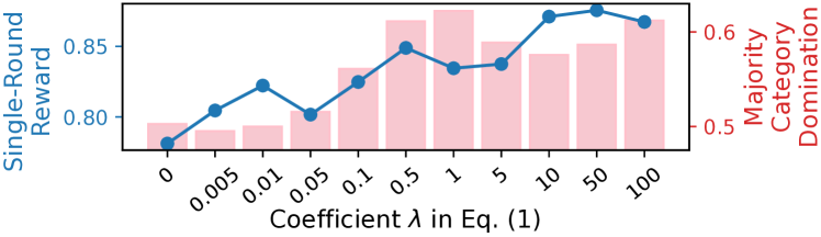
Figure 3. Effect of conservatism in recommendation.

We show the effect of conservatism of MOPO by varying the coefficient $\lambda$ of Eq. (1). The results on the KuaiRec dataset are shown in Fig. 3. With increasing $\lambda$, the model receives a higher single-round reward (the blue line), which means the policy captures users’ interest more accurately. On the other hand, MCD also increases (the red bars), which means the recommended items tend to be the most popular categories (those cover 80% items) in training data. I.e., the more conservative the policy is, the stronger the Matthew effect becomes.

When the results narrow down to these categories, users’ satisfaction will be hurt and the interaction process terminates early, which results in low cumulative rewards over the interaction sequence. More details will be described in Section 6.

5.3. Solution: Re-design the Penalty

To address this issue, we consider a more sophisticated manner to design the penalty term $p(s,a)$ in Eq. (1). We dissect the mismatch function in Eq. (4) as:

(7) $$\begin{split}|G_{\widehat{M}}^{\pi}(s,a)|\leq&\gamma|\mathbb{E}_{\hat{r}\sim\widehat{R}}[V_{M}^{\pi}(f_{\omega}(s,a,\hat{r}))]-\mathbb{E}_{r\sim R}[V_{M}^{\pi}(f_{\omega}(s,a,r))]|\\ &+|\mathbb{E}_{\hat{r}\sim\widehat{R}}r-\mathbb{E}_{r\sim R}r|\coloneqq\gamma d_{V}(\widehat{R},R)+d_{1}(\widehat{R},R),\end{split}$$

where $d_{1}(\widehat{R},R)$ represents the deviation of estimated reward $\widehat{R}$ from true reward $R$, $d_{V}(\widehat{R},R)$ measures the difference between the value functions $V_{M}^{\pi}$ of next state calculated offline (via $\widehat{R}$) and online (via $R$). Both of them can be seen as specific metrics measuring the distance between $\widehat{R}$ and $R$. While $d_{1}(\widehat{R},R)$ is straightforward, $d_{V}(\widehat{R},R)$ considers the long-term effect on offline learning and is hard to estimate. Based on the aforementioned analysis, a pessimistic reward model $\widehat{R}$ in MOPO will amplify the Matthew effect that reduces long-term satisfaction, thus resulting in a large $d_{V}(\widehat{R},R)$.

An intuitive way to solve this dilemma is to introduce exploration on states with high entropy of the logging policy. Without access to online user feedback, we can only conduct the counterfactual exploration in the offline data.

$\bullet$ An illustrative example. To illustrate the idea, we give an example in Fig. 4. The goal is to estimate a user’s preferences given the logged data induced by a behavior policy. In reality, the distribution of the logged data is dependent on the policies of previous recommenders. For convenience, we use a Gaussian distribution as the behavior policy in Fig. 4(a). Since previous recommenders cannot precisely reflect users’ ground-truth preferences, there is always a deviation between the behavior policy (the red line) and users’ ground-truth preferences (the blue line).

Besides, as the items are not equally exposed in the behavior policy, there will be high uncertainty in estimating the rarely appeared items (as shown in the filled area). Offline RL methods emphasize conservatism in estimation and penalize the uncertain samples, which results in the distribution that narrows down the preferences to these dominated items (the green line). This is how the Matthew effect appears.

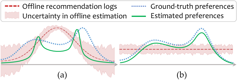
Figure 4. Estimating user preferences using behavior policies with a Gaussian distribution and a uniform distribution.

By contrast, using a uniform distribution to collect data can prevent biases and reduce uncertainty (Fig. 4(b)). Ideally, a policy learned on sufficient data collected uniformly can capture unbiased user preferences and produce recommendations without the Matthew effect, i.e., $\gamma d_{V}(\widehat{R},R)+d_{1}(\widehat{R},R)$ can reduce to $0$.

Therefore, an intuitive way to design penalty term $p(s,a)$ is to add a term: the discrepancy of behavior between the uniform distribution $\pi_{u}(\cdot|s)$ and the behavior policy $\pi_{\beta}(\cdot|s)$ given state $s$. We use the Kullback–Leibler divergence $D_{KL}(\pi_{\beta}(\cdot|s)||\pi_{u}(\cdot|s))$ to measure the distance, which can be written as:

(8) $$P_{E}\text{ := } -D_{KL}(\pi_{\beta}(\cdot|s)||\pi_{u}(\cdot|s))$$

$$= -\mathbb{E}_{a\sim\pi_{\beta}(\cdot|s)}[\log(\pi_{\beta}(a|s))-\log(\pi_{u}(a|s))]$$

$$= ~{}\mathcal{H}(\pi_{\beta}(\cdot|s))-\log(|\mathcal{A}|),$$

where $|\mathcal{A}|$ is a constant representing the number of items. Hence, the term $P_{E}$ depends on the entropy of the behavior policy $\pi_{\beta}(\cdot|s)$ given state $s$. The modified penalty term can be written as $p(s,a)=P_{U}+P_{E}$, and the modified reward model will be formulated as:

(9) $$\tilde{r}(s,a)=\hat{r}(s,a)-\lambda_{1}P_{U}+\lambda_{2}P_{E}.$$

Except for penalizing high uncertainty areas, the new model also penalizes policies with a low entropy at state $s$. Intuitively, if the behavior policy $\pi_{\beta}(\cdot|s)$ recommended only a few items at state $s$, then the true user preferences at state $s$ may be unrevealed. Under such circumstances, the entropy term $\mathcal{H}(\pi_{\beta}(\cdot|s))$ is low, hence we penalize the estimated reward $\hat{r}(s,a)$ by a large $P_{E}$.

The entropy penalizer does not depend on the chosen action but only on the state in which the agent is. Which means the effect of this penalty will be indirect and penalize actions that lead to less diverse states, because of the long-term optimization. Hence, The learned policy achieves the counterfactual exploration in the offline data, which in turn counteracts the Matthew effect in offline RL.

5.4. The DORL Method

Now, we provide a practical implementation motivated by the analysis above. The proposed model is named Debiased model-based Offline RL (DORL) model, whose framework is illustrated in Fig. 6.

$\bullet$ Penalty on entropy. We introduce how to compute $P_{E}$ in the entropy penalizer module.

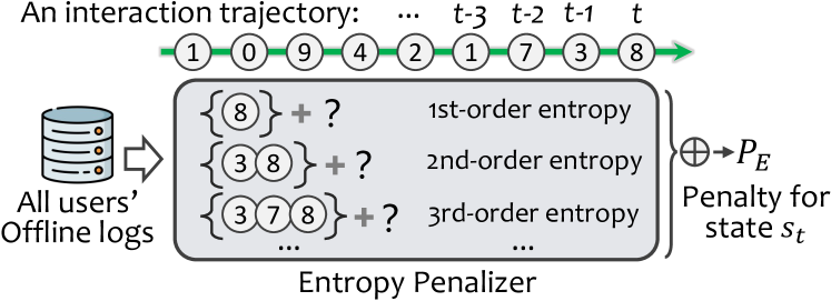
Figure 5. Illustration of the mechanism of entropy penalizer.

Fig. 5 shows a trajectory of the interaction process, where the current action at time $t$ is to recommend item 8. We define $P_{E}$ in Eq. (9) to be the summation of $k$-order entropy ($k=1,2,\cdots$). For example, when $k=3$, we search all users’ recommendation logs to collect all continuous sub-sequences with pattern $[\{3,7,8\},?]$, where “$?$” can match any item, and $\{3,7,8\}$ is a sorted set that can cover all of its enumeration, e.g., $[8,3,7]$ or $[7,3,8]$. On these sub-sequences, we can count the frequencies of action “$?$” to estimate the entropy of behavior policy $\pi_{\beta}$ given the previous three recommended items. Without losing generality, we normalize the entropy to range $(0,1]$.

$\bullet$ Penalty on uncertainty. We penalize both the epistemic uncertainty of the reward model and the aleatoric uncertainty of offline data. We use the variance of $K$ ensemble reward models $\{\widehat{R}_{\theta_{k}},k=1,2,\cdots,K\}$ to capture the epistemic uncertainty, which is commonly used to capture the uncertainty of the model in offline RL (Levine et al., 2020). Aleatoric uncertainty is data-dependent (Kendall and Gal, 2017). By formulating the user model as a Gaussian probabilistic model (GPM), we can directly predict the variance of the reward and take this predicted variance as aleatoric uncertainty. For the $k$-th model $\widehat{R}_{\theta_{k}}$, the loss function is:

(10) $$\mathcal{L}(\theta_{k})=\frac{1}{N}\sum_{i=1}^{N}\frac{1}{2\sigma^{2}_{\theta_{k}}(x_{i})}\|y_{i}-f_{\theta_{k}}(x_{i})\|^{2}+\frac{1}{2}\log\sigma^{2}_{\theta_{k}}(x_{i}),$$

where $N$ is the number of samples, $f_{\theta_{k}}(x_{i})$ and $\sigma^{2}_{\theta_{k}}(x_{i})$ are the predicted mean and variance of sample $x_{i}$, respectively. By combining epistemic uncertainty and aleatoric uncertainty, we formulate the uncertainty pernalizer $P_{U}$ in Eq. (9) as: $P_{U}\text{ := }\max_{k\in\{1,2,\cdots,K\}}\sigma^{2}_{\theta_{k}}.$ We define the fitted reward $\hat{r}$ as the mean of $K$ ensemble models: $\hat{r}(s,a)=\frac{1}{K}\sum_{k}{f_{\theta_{k}}(s,a)}$. The final modified reward $\tilde{r}(s,a)$ will be computed by Eq. (9).

The framework of the proposed DORL model is illustrated in Fig. 6. Without losing generality, we use DeepFM (Guo et al., 2017) as the backbone for the user model and implement the actor-critic method (Konda and Tsitsiklis, 1999) as the RL policy.

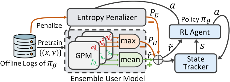
Figure 6. Illustration of Debiased Model-based Offline RL-based Recommendation (DORL) framework.

The state tracker $f_{\omega}(s,a,r)$ is a network modeling the transition function $T(s,a,s^{\prime})=P(s_{t+1}=s^{\prime}|s_{t}=s,a_{t}=a)$. It can be implemented as any sequential model such as recurrent neural network (RNN)-based models (Wang et al., 2022a), Convolutional models (Tang and Wang, 2018; Yuan et al., 2019), Transformer-based methods (Kang and McAuley, 2018; Gao et al., 2022a; Xin et al., 2022). Huang et al. (2022) investigated the performances of different state encoders in RL-based recommenders. We use a naive average layer as the state tracker since it requires the least training time but nonetheless outperforms many complex encoders (Huang et al., 2022). It can be written as:

(11) $$\vec{s}_{t+1}\coloneqq\frac{1}{N}\sum^{t}_{n=t-N+1}[\vec{e}_{a_{n}}\oplus\tilde{r}_{n}],$$

where $\oplus$ is the concatenation symbol, $\vec{s}_{t+1}$ is the vector representing the state at time $t+1$, $\vec{e}_{a_{n}}$ is the embedding vector of action $a_{n}$. $\tilde{r}_{n}$ is the reward value calculated by Eq. (9) and we normalize it to range (0,1] here. $N$ is the window size reflecting how many previous item-reward pairs are calculated.

6. Experiments

We introduce how we evaluate the proposed DORL model in the interactive recommendation setting. We want to investigate the following questions:

• (RQ1) How does DORL perform compared to state-of-the-art offline RL methods in the interactive recommendation setting?

• (RQ2) To what extent can DORL alleviate the Matthew effect and pursue long-term user experience?

• (RQ3) How does DORL perform in different environments with different user tolerance to repeated content?

6.1. Experimental Setup

We introduce the experimental settings with regard to environments and state-of-the-art offline RL methods.

6.1.1. Recommendation Environments

As mentioned in Section 2.2, in the interactive recommendation setting, we are interested in users’ long-term satisfaction rather than users’ fitting capabilities (Deffayet et al., 2023). Traditional recommendation datasets are too sparse or lack necessary information (e.g., timestamps, explicit feedback, item categories) to evaluate the interactive recommender systems. We create two recommendation environments on two recently-proposed datasets, KuaiRec and KuaiRand-Pure, which contain high-quality logs.

KuaiRec (Gao et al., 2022b) is a video dataset that contains a fully-observed user-item interaction matrix where 1,411 users have viewed all 3,327 videos and left feedback. By taking the fully-observed matrix as users’ true interest, we can give a reward for the model’s every recommendation (without missing entries like other datasets). We use the normalized viewing time (i.e., the ratio of viewing time to the video length) as the online reward.

KuaiRand-Pure (Gao et al., 2022c) is a video dataset that inserted 1,186,059 random recommendations involving 7,583 items into 27,285 users’ standard recommendation streams. These randomly exposed data can reflect users’ unbiased preferences, from which we can complete the matrix to emulate the fully-observed matrix in KuaiRec. This is an effective way to evaluate RL-based recommendation (Huang et al., 2022, 2020). We use the “is_click” signal to indicate users’ ground-truth interest, i.e., as the online reward.

In Section 3, we have shown that users’ experience can be hurt by the Matthew effect. To let the environments reflect this phenomenon, we follow (Gao et al., 2022a; Xu et al., 2022) to introduce a quit mechanism: when the model recommends more than $M$ items with the same category in previous $N$ rounds, the interaction terminates. Note that the same item will not be recommended twice in an interaction sequence. Since we evaluate the model via the cumulative rewards $\sum_{t}r_{t}$ over the interaction trajectory, quitting early (due to the Matthew effect) will lead to inferior performances. For now, the two environments can play the same role as the online users. Therefore, we can evaluate the model as the process shown in Fig. 1 (b).

The evaluation environments are used for assessing models and they are not available in the training stage. For the training purpose, both KuaiRec and KuaiRand provide additional recommendation logs. The statistics of the training data are illustrated in Table 1.

Table 1. Statistics of two datasets.

Datasets	Usage	#Users	#Items	#Interactions	#Categories
KuaiRec	Train	7,176	10,728	12,530,806	31
	Test	1,411	3,327	4,676,570	31
KuaiRand	Train	27,285	7,551	1,436,609	46
	Test	27,285	7,583	1,186,059	46

6.1.2. Baselines

We select two naive bandit-based algorithms, four model-free offline RL methods, and four model-based offline RL methods (including ours) in evaluation. We use the DeepFM model (Guo et al., 2017) as the backbone in the two bandit methods and four model-based methods. These baselines are:

• $\epsilon$-greedy, a naive bandit-based policy that outputs a random result with probability $\epsilon$ or outputs the deterministic results of DeepFM with probability $1-\epsilon$.

• UCB, a naive bandit-based policy that maintains an upper confidence bound for each item and follows the principle of optimism in the face of uncertainty.

• SQN, or Self-Supervised Q-learning (Xin et al., 2020), contains two output layers (heads): one for the cross-entropy loss and the other for RL. We use the RL head to generate final recommendations.

• BCQ, or Batch-Constrained deep Q-learning (Fujimoto et al., 2019b), adapts the conventional deep Q-learning to batch RL. We use the discrete-action version (Fujimoto et al., 2019a), whose core idea is to reject these uncertain data and update the policy using only the data of high confidence.

• CQL, or Conservative Q-Learning (Kumar et al., 2020), is a model-free RL method that adds a Q-value regularizer on top of an actor-critic policy.

• CRR, or Critic Regularized Regression (Wang et al., 2020b), is a model-free RL method that learns the policy by avoiding OOD actions.

• MBPO, a vanilla model-based policy optimization method that uses DeepFM as the user model to train an actor-critic policy.

• IPS (Swaminathan and Joachims, 2015) is a well-known statistical technique adjusting the target distribution by re-weighting each sample in the collected data. We implement IPS in a DeepFM-based user model, then learn the policy using an actor-critic method.

• MOPO, a model-based offline policy optimization method (Yu et al., 2020) that penalizes the uncertainty of the DeepFM-based user model and then learns an actor-critic policy.

6.2. Overall Performance Comparison (RQ1)

We evaluate all methods in two environments. For the four model-based RL methods (MBPO, IPS, MOPO, and our DORL), we use the same DeepFM model as the user model and fixed its parameters to make sure the difference comes only from the policies. We use the grid search technique on the key parameters to tune all methods in the two environments. For DORL, we search the combination of two key parameters $\lambda_{1}$ and $\lambda_{2}$ in Eq. (9). Both of them are searched in $\{0.001,0.005,0.01,0.05,0.1,0.5,1.0,5,10,50,100\}$. We report the results with $\lambda_{1}=0.01,\lambda_{2}=0.05$ for KuaiRand and $\lambda_{1}=0.05,\lambda_{2}=5$ for KuaiRec. All methods in two environments are evaluated with the quit parameters: $M=0,N=4$, and the maximum round is set to 30. The results are the average metrics of $100$ interaction trajectories.

Figure 7. Results of all methods in two environments.

Table 2. Average Results of all methods in the two environments. (Bold: Best; underline: runner-up).

Methods	KuaiRec				KuaiRand
	$\text{R}_{\text{tra}}$	$\text{R}_{\text{each}}$	Length	MCD	$\text{R}_{\text{tra}}$	$\text{R}_{\text{each}}$	Length	MCD
UCB	$3.606\pm 0.609$	$0.853\pm 0.114$	$4.219\pm 0.389$	$0.811\pm 0.058$	$1.651\pm 0.152$	$0.372\pm 0.028$	$4.431\pm 0.212$	$0.789\pm 0.024$
$\epsilon$-greedy	$3.515\pm 0.731$	$0.828\pm 0.129$	$4.219\pm 0.405$	$0.823\pm 0.048$	$1.711\pm 0.126$	$0.351\pm 0.025$	$4.880\pm 0.270$	$0.773\pm 0.024$
SQN	$4.673\pm 1.215$	$\mathbf{0.913\pm 0.055}$	$5.111\pm 1.288$	$0.686\pm 0.093$	$0.912\pm 0.929$	$0.182\pm 0.058$	$4.601\pm 3.712$	$0.621\pm 0.187$
CRR	$4.163\pm 0.253$	$0.895\pm 0.037$	$4.654\pm 0.215$	$0.865\pm 0.017$	$1.481\pm 0.124$	$0.226\pm 0.015$	$6.561\pm 0.352$	$0.733\pm 0.019$
CQL	$2.506\pm 1.767$	$0.684\pm 0.228$	$3.224\pm 1.365$	$0.386\pm 0.385$	$2.032\pm 0.107$	$0.226\pm 0.012$	$9.000\pm 0.000$	$0.778\pm 0.000$
BCQ	$2.123\pm 0.081$	$0.708\pm 0.027$	$3.000\pm 0.000$	$0.667\pm 0.000$	$0.852\pm 0.052$	$0.425\pm 0.016$	$2.005\pm 0.071$	$0.998\pm 0.024$
MBPO	$12.043\pm 1.312$	$0.770\pm 0.029$	$15.646\pm 1.637$	$0.362\pm 0.047$	$10.933\pm 0.946$	$0.431\pm 0.021$	$25.345\pm 1.819$	$0.306\pm 0.040$
IPS	$12.833\pm 1.353$	$0.767\pm 0.023$	$16.727\pm 1.683$	$\mathbf{0.215\pm 0.064}$	$3.629\pm 0.676$	$0.216\pm 0.014$	$16.821\pm 3.182$	$\mathbf{0.201\pm 0.116}$
MOPO	$11.427\pm 1.750$	$0.892\pm 0.051$	$12.809\pm 1.850$	$0.479\pm 0.062$	$10.934\pm 0.963$	$\mathbf{0.437\pm 0.019}$	$25.002\pm 1.891$	$0.343\pm 0.029$
Ours	$\mathbf{20.494\pm 2.671}$	$0.767\pm 0.026$	$\mathbf{26.712\pm 3.419}$	$0.379\pm 0.015$	$\mathbf{11.850\pm 1.036}$	$0.428\pm 0.022$	$\mathbf{27.609\pm 2.121}$	$0.296\pm 0.036$

The results are shown in Fig. 7, where all policies are learned with 200 epochs. After learning in each epoch, we will evaluate all methods with $100$ episodes (i.e., interaction trajectories) in the two interactive environments. The first row shows the cumulative reward, which directly reflects the long-term satisfaction in our interactive recommendation setting. The second row and third rows dissect the cumulative reward into two parts: the length of the interaction trajectory and the single-round reward, respectively. For a better comparison, we average the results in 200 epochs and show them in Table 2. Besides the three metrics, we also report the majority category domination (MCD) in Table 2.

From the results, we observe that the four model-based RL methods (MBPO, IPS, MOPO, and DORL) significantly outperform the four model-free RL methods (SQN, CRR, CQL, and BCQ) with respect to trajectory length and cumulative reward. This is because model-based RL is much more sample efficient than model-free RL. In recommendation, the training data is highly sparse. Model-free RL learns directly from the recommendation logs that we have split into different sequences according to the exit rule described above. However, it is extremely difficult to capture the exit mechanism from the sparse logs. By contrast, the model-based RL can leverage the user model to construct as many interaction sequences as possible during training, which guarantees that the policy can distill useful knowledge from the limited offline samples. That is why we embrace model-based RL in recommendation.

For model-based RL methods, MOPO shows an obvious improvement compared to the vanilla method MBPO in terms of single-round reward. It is because MBPO does not consider the OOD actions in the offline data that will incur extrapolation errors in the policy. MOPO introduces the uncertainty penalizer to make the policy pay more attention to the samples of high confidence, which in turn makes the policy capture users’ interest more precisely. However, MOPO sacrifices many unpopular items because they appear less frequently and are considered uncertain samples. Therefore, the average length decreases, which in turn reduces the cumulative reward. Our method DORL overcomes this problem. From Fig. 7, we observe that DORL attains the maximal average cumulative reward after several epochs in both KuaiRec and KuaiRand due to that it reaches the largest interaction length. Compared to MOPO and MBPO, DORL sacrifices a little bit of the single-round reward due to its counterfactual exploration philosophy, meanwhile, this greatly improves the diversity and enlarges the length of interactions due. Therefore, it achieves the goal of maximizing users’ long-term experiences. After enhancing the vanilla MBPO with the IPS technique, the learned user model gives adjustments to the distribution of training data by re-weighting all items. IPS obtains a satisfactory performance in KuaiRec but receives abysmal performances in KuaiRand. This is due to its well-known high variance issue can incur estimation errors. Compared to IPS’s hard debiased mechanism, DORL’s soft debiased method is more suitable for model-based RL in recommendation.

For model-free RL methods, As discussed above, four model-free methods fail in two datasets due to limited offline samples. Though they can capture users’ interest by returning a high single-round reward (e.g., SQN and CRR in KuaiRec, and BCQ in KuaiRand), they cannot maintain a long interaction trajectory. For example, BCQ updates its policy only on those samples with high confidence, which results in a severe Matthew effect in the recommendation results (reflected by high MCD and short length). SQN’s performance oscillates with the largest magnitude since its network is updated by two heads. The RL head serves as a regularizer to the self-supervised head. When the objectives of the two heads conflict with each other, the performance becomes unstable. Therefore, these methods are not suitable for recommendation where offline data are sparse.

As for the naive bandit methods, UCB and $\epsilon$-greedy, they are designed to explore and exploit the optimal actions for the independent and identically distributed (IID) data. They do not even possess the capability to optimize long-term rewards at all. Therefore, they are inclined to recommend the same items when the model finishes exploring offline data, which leads to high MCD and short interactions. These naive policies are not suitable for pursuing long-term user experiences in recommendation.

6.3. Results on alleviating Matthew effect (RQ2)

Figure 8. Effect of penalizing entropy.

We have shown in Fig. 3 that penalizing uncertainty will result in the Matthew effect in recommendation. More specifically, increasing $\lambda_{1}$ can make the recommended items to be the most dominant ones in the training set, which results in a high MCD value. Here, we show how the introduced “counterfactual” exploration mechanism helps alleviate this effect. We conduct the experiments for different combinations of $(\lambda_{1},\lambda_{2})$ as described above, then we average the results along the $\lambda_{1}$ to show the influence of $\lambda_{2}$ alone.

The results are shown in Fig. 8. Obviously, increasing $\lambda_{2}$ can lengthen the interaction process and reduce majority category domination. I.e., When we penalize the entropy of behavior policy hard, (1) the recommender does not repeat the items with the same categories; (2) the recommended results will be diverse instead of focusing on dominated items. The results show the effectiveness of penalizing entropy in DORL in alleviating the Matthew effect.

6.4. Results with different environments (RQ3)

To validate that DORL can work robustly in different environment settings, we vary the window size $N$ in the exit mechanism and fix $M=10$ during the evaluation. The results are shown in Fig. 9. We only visualize the most important metric: the cumulative reward. When $N$ is small ($N=1$), other model-based methods can surpass our DORL. When $N$ gets larger ($N>3$), users’ tolerance for similar content (i.e., items with the same category) becomes lower, and the interaction process comes to be easier to terminate. Under such a circumstance, DORL outperforms all other policies, which demonstrates the robustness of DORL in different environments.

Figure 9. Results under different ending conditions

7. Conclusion

We point out that conservatism in offline RL can incur the Matthew effect in recommendation. We conduct studies to show that the Matthew effect hurts users’ long-term experiences in both the music and video datasets. Through theoretical analysis of the model-based RL framework, we show that the reason for amplifying the Matthew effect is the philosophy of suppressing uncertain samples. It inspires us to add a penalty term to make the policy emphasize the data induced by the behavior policies with high entropy. This will reintroduce the exploration mechanism that conservatism has suppressed, which alleviates the Matthew effect.

In the future, when fitting user interests is not a bottleneck anymore, researchers could consider higher-level goals, such as pursuing users’ long-term satisfaction (Zhang et al., 2022) or optimizing social utility (Ge et al., 2022). With the increase in high-quality offline data, we believe that offline RL can be better adapted to recommender systems to achieve these goals. During this process, many interesting yet challenging issues (such as the Matthew effect in this work) will be raised. After addressing these issues, we can create more intelligent recommender systems that benefit society.

References

- (1)
- Afsar et al. (2022) M Mehdi Afsar, Trafford Crump, and Behrouz Far. 2022. Reinforcement Learning based Recommender Systems: A Survey. Comput. Surveys 55, 7 (2022), 1–38.
- Agarwal et al. (2020) Rishabh Agarwal, Dale Schuurmans, and Mohammad Norouzi. 2020. An optimistic perspective on offline reinforcement learning. In International Conference on Machine Learning (ICML ’20). PMLR, 104–114.
- Anderson et al. (2020) Ashton Anderson, Lucas Maystre, Ian Anderson, Rishabh Mehrotra, and Mounia Lalmas. 2020. Algorithmic Effects on the Diversity of Consumption on Spotify. In Proceedings of The Web Conference 2020 (Taipei, Taiwan) (WWW ’20). 2155–2165.
- Cai et al. (2023a) Qingpeng Cai, Shuchang Liu, Xueliang Wang, Tianyou Zuo, Wentao Xie, Bin Yang, Dong Zheng, Peng Jiang, and Kun Gai. 2023a. Reinforcing User Retention in a Billion Scale Short Video Recommender System. arXiv preprint arXiv:2302.01724 (2023).
- Cai et al. (2023b) Qingpeng Cai, Zhenghai Xue, Chi Zhang, Wanqi Xue, Shuchang Liu, Ruohan Zhan, Xueliang Wang, Tianyou Zuo, Wentao Xie, Dong Zheng, et al. 2023b. Two-Stage Constrained Actor-Critic for Short Video Recommendation. arXiv preprint arXiv:2302.01680 (2023).
- Chen et al. (2019) Minmin Chen, Alex Beutel, Paul Covington, Sagar Jain, Francois Belletti, and Ed H. Chi. 2019. Top-K Off-Policy Correction for a REINFORCE Recommender System. In Proceedings of the Twelfth ACM International Conference on Web Search and Data Mining (Melbourne VIC, Australia) (WSDM ’19). 456–464.
- Chen et al. (2022) Minmin Chen, Can Xu, Vince Gatto, Devanshu Jain, Aviral Kumar, and Ed Chi. 2022. Off-Policy Actor-Critic for Recommender Systems. In Proceedings of the 16th ACM Conference on Recommender Systems (Seattle, WA, USA) (RecSys ’22). 338–349.
- Deffayet et al. (2023) Romain Deffayet, Thibaut Thonet, Jean-Michel Renders, and Maarten de Rijke. 2023. Offline Evaluation for Reinforcement Learning-based Recommendation: A Critical Issue and Some Alternatives. arXiv preprint arXiv:2301.00993 (2023).
- Ebert et al. (2018) Frederik Ebert, Chelsea Finn, Sudeep Dasari, Annie Xie, Alex Lee, and Sergey Levine. 2018. Visual foresight: Model-based deep reinforcement learning for vision-based robotic control. arXiv preprint arXiv:1812.00568 (2018).
- Fujimoto et al. (2019a) Scott Fujimoto, Edoardo Conti, Mohammad Ghavamzadeh, and Joelle Pineau. 2019a. Benchmarking batch deep reinforcement learning algorithms. arXiv preprint arXiv:1910.01708 (2019).
- Fujimoto et al. (2019b) Scott Fujimoto, David Meger, and Doina Precup. 2019b. Off-Policy Deep Reinforcement Learning without Exploration. In Proceedings of the 36th International Conference on Machine Learning (Proceedings of Machine Learning Research, Vol. 97), Kamalika Chaudhuri and Ruslan Salakhutdinov (Eds.). 2052–2062.
- Gao et al. (2022a) Chongming Gao, Wenqiang Lei, Jiawei Chen, Shiqi Wang, Xiangnan He, Shijun Li, Biao Li, Yuan Zhang, and Peng Jiang. 2022a. CIRS: Bursting Filter Bubbles by Counterfactual Interactive Recommender System. arXiv preprint arXiv:2204.01266 (2022).
- Gao et al. (2021) Chongming Gao, Wenqiang Lei, Xiangnan He, Maarten de Rijke, and Tat-Seng Chua. 2021. Advances and Challenges in Conversational Recommender Systems: A Survey. AI Open 2 (2021), 100–126.
- Gao et al. (2022b) Chongming Gao, Shijun Li, Wenqiang Lei, Jiawei Chen, Biao Li, Peng Jiang, Xiangnan He, Jiaxin Mao, and Tat-Seng Chua. 2022b. KuaiRec: A Fully-Observed Dataset and Insights for Evaluating Recommender Systems. In Proceedings of the 31st ACM International Conference on Information & Knowledge Management (Atlanta, GA, USA) (CIKM ’22). 540–550. https://doi.org/10.1145/3511808.3557220
- Gao et al. (2022c) Chongming Gao, Shijun Li, Yuan Zhang, Jiawei Chen, Biao Li, Wenqiang Lei, Peng Jiang, and Xiangnan He. 2022c. KuaiRand: An Unbiased Sequential Recommendation Dataset with Randomly Exposed Videos. In Proceedings of the 31st ACM International Conference on Information and Knowledge Management (Atlanta, GA, USA) (CIKM ’22). 3953–3957. https://doi.org/10.1145/3511808.3557624
- Gao et al. (2022d) Zhaolin Gao, Tianshu Shen, Zheda Mai, Mohamed Reda Bouadjenek, Isaac Waller, Ashton Anderson, Ron Bodkin, and Scott Sanner. 2022d. Mitigating the Filter Bubble While Maintaining Relevance: Targeted Diversification with VAE-Based Recommender Systems. In Proceedings of the 45th International ACM SIGIR Conference on Research and Development in Information Retrieval (Madrid, Spain) (SIGIR ’22). 2524–2531.
- Ge et al. (2022) Yingqiang Ge, Xiaoting Zhao, Lucia Yu, Saurabh Paul, Diane Hu, Chu-Cheng Hsieh, and Yongfeng Zhang. 2022. Toward Pareto Efficient Fairness-Utility Trade-off in Recommendation through Reinforcement Learning. In Proceedings of the Fifteenth ACM International Conference on Web Search and Data Mining (Virtual Event, AZ, USA) (WSDM ’22). 316–324.
- Gilotte et al. (2018) Alexandre Gilotte, Clément Calauzènes, Thomas Nedelec, Alexandre Abraham, and Simon Dollé. 2018. Offline A/B Testing for Recommender Systems. In WSDM ’18. 198–206.
- Guo et al. (2017) Huifeng Guo, Ruiming Tang, Yunming Ye, Zhenguo Li, and Xiuqiang He. 2017. DeepFM: A Factorization-Machine Based Neural Network for CTR Prediction. In Proceedings of the 26th International Joint Conference on Artificial Intelligence (Melbourne, Australia) (IJCAI’17). 1725–1731.
- Hansen et al. (2021) Christian Hansen, Rishabh Mehrotra, Casper Hansen, Brian Brost, Lucas Maystre, and Mounia Lalmas. 2021. Shifting Consumption towards Diverse Content on Music Streaming Platforms. In Proceedings of the 14th ACM International Conference on Web Search and Data Mining (Virtual Event, Israel) (WSDM ’21). 238–246.
- Ho and Ermon (2016) Jonathan Ho and Stefano Ermon. 2016. Generative Adversarial Imitation Learning. In Advances in Neural Information Processing Systems (NeurIPS ’16, Vol. 29), D. Lee, M. Sugiyama, U. Luxburg, I. Guyon, and R. Garnett (Eds.).
- Huang et al. (2022) Jin Huang, Harrie Oosterhuis, Bunyamin Cetinkaya, Thijs Rood, and Maarten de Rijke. 2022. State Encoders in Reinforcement Learning for Recommendation: A Reproducibility Study. In Proceedings of the 45th International ACM SIGIR Conference on Research and Development in Information Retrieval (Madrid, Spain) (SIGIR ’22). 2738–2748.
- Huang et al. (2020) Jin Huang, Harrie Oosterhuis, Maarten de Rijke, and Herke van Hoof. 2020. Keeping Dataset Biases out of the Simulation: A Debiased Simulator for Reinforcement Learning Based Recommender Systems. In RecSys ’20. 190–199.
- Jeunen and Goethals (2021) Olivier Jeunen and Bart Goethals. 2021. Pessimistic Reward Models for Off-Policy Learning in Recommendation. In Proceedings of the 15th ACM Conference on Recommender Systems (Amsterdam, Netherlands) (RecSys ’21). 63–74.
- Kang and McAuley (2018) Wang-Cheng Kang and Julian McAuley. 2018. Self-attentive sequential recommendation. In International Conference on Data Mining (ICDM ’18). IEEE, 197–206.
- Kendall and Gal (2017) Alex Kendall and Yarin Gal. 2017. What Uncertainties Do We Need in Bayesian Deep Learning for Computer Vision?. In Proceedings of the 31st International Conference on Neural Information Processing Systems (Long Beach, California, USA) (NeurIPS ’17). 5580–5590.
- Kidambi et al. (2020) Rahul Kidambi, Aravind Rajeswaran, Praneeth Netrapalli, and Thorsten Joachims. 2020. MOReL: Model-Based Offline Reinforcement Learning. In Advances in Neural Information Processing Systems (NeurIPS ’20, Vol. 33), H. Larochelle, M. Ranzato, R. Hadsell, M.F. Balcan, and H. Lin (Eds.). 21810–21823.
- Konda and Tsitsiklis (1999) Vijay Konda and John Tsitsiklis. 1999. Actor-critic algorithms. Advances in neural information processing systems 12 (1999).
- Kostrikov et al. (2022) Ilya Kostrikov, Ashvin Nair, and Sergey Levine. 2022. Offline Reinforcement Learning with Implicit Q-Learning. In International Conference on Learning Representations (ICLR ’22).
- Kumar et al. (2019) Aviral Kumar, Justin Fu, Matthew Soh, George Tucker, and Sergey Levine. 2019. Stabilizing off-policy q-learning via bootstrapping error reduction. Advances in Neural Information Processing Systems 32 (2019).
- Kumar et al. (2020) Aviral Kumar, Aurick Zhou, George Tucker, and Sergey Levine. 2020. Conservative Q-Learning for Offline Reinforcement Learning. In Advances in Neural Information Processing Systems (NeurIPS ’20, Vol. 33), H. Larochelle, M. Ranzato, R. Hadsell, M.F. Balcan, and H. Lin (Eds.). 1179–1191.
- Lei et al. (2021) Wenqiang Lei, Chongming Gao, and Maarten de Rijke. 2021. RecSys 2021 Tutorial on Conversational Recommendation: Formulation, Methods, and Evaluation (RecSys ’21). Association for Computing Machinery, New York, NY, USA, 842–844. https://doi.org/10.1145/3460231.3473325
- Levine et al. (2020) Sergey Levine, Aviral Kumar, George Tucker, and Justin Fu. 2020. Offline reinforcement learning: Tutorial, review, and perspectives on open problems. arXiv preprint arXiv:2005.01643 (2020).
- Liang et al. (2021) Yile Liang, Tieyun Qian, Qing Li, and Hongzhi Yin. 2021. Enhancing Domain-Level and User-Level Adaptivity in Diversified Recommendation. In Proceedings of the 44th International ACM SIGIR Conference on Research and Development in Information Retrieval (Virtual Event, Canada) (SIGIR ’21). 747–756.
- Liu et al. (2023) Shuchang Liu, Qingpeng Cai, Bowen Sun, Yuhao Wang, Ji Jiang, Dong Zheng, Kun Gai, Peng Jiang, Xiangyu Zhao, and Yongfeng Zhang. 2023. Exploration and Regularization of the Latent Action Space in Recommendation. arXiv preprint arXiv:2302.03431 (2023).
- Liu and Huang (2021) Ying Chieh Liu and Min Qi Huang. 2021. Examining the Matthew Effect on YouTube Recommendation System. In International Conference on Technologies and Applications of Artificial Intelligence (TAAI ’21). 146–148. https://doi.org/10.1109/TAAI54685.2021.00035
- Luo et al. (2018) Yuping Luo, Huazhe Xu, Yuanzhi Li, Yuandong Tian, Trevor Darrell, and Tengyu Ma. 2018. Algorithmic framework for model-based deep reinforcement learning with theoretical guarantees. arXiv preprint arXiv:1807.03858 (2018).
- Schedl (2016) Markus Schedl. 2016. The LFM-1b Dataset for Music Retrieval and Recommendation. In Proceedings of the 2016 ACM on International Conference on Multimedia Retrieval (New York, New York, USA) (ICMR ’16). 103–110.
- Swaminathan and Joachims (2015) Adith Swaminathan and Thorsten Joachims. 2015. Counterfactual Risk Minimization: Learning from Logged Bandit Feedback. In International Conference on Machine Learning (ICML ’15). PMLR, 814–823.
- Tang and Wang (2018) Jiaxi Tang and Ke Wang. 2018. Personalized Top-N Sequential Recommendation via Convolutional Sequence Embedding. In Proceedings of the Eleventh ACM International Conference on Web Search and Data Mining (Marina Del Rey, CA, USA) (WSDM ’18). 565–573.
- Tomlein et al. (2021) Matus Tomlein, Branislav Pecher, Jakub Simko, Ivan Srba, Robert Moro, Elena Stefancova, Michal Kompan, Andrea Hrckova, Juraj Podrouzek, and Maria Bielikova. 2021. An Audit of Misinformation Filter Bubbles on YouTube: Bubble Bursting and Recent Behavior Changes. In RecSys ’21. 1–11.
- Wang et al. (2018) Hao Wang, Zonghu Wang, and Weishi Zhang. 2018. Quantitative analysis of Matthew effect and sparsity problem of recommender systems. In 2018 IEEE 3rd International Conference on Cloud Computing and Big Data Analysis (ICCCBDA). 78–82. https://doi.org/10.1109/ICCCBDA.2018.8386490
- Wang et al. (2020a) Ruosong Wang, Dean P Foster, and Sham M Kakade. 2020a. What are the statistical limits of offline RL with linear function approximation? arXiv preprint arXiv:2010.11895 (2020).
- Wang et al. (2022a) Shiqi Wang, Chongming Gao, Min Gao, Junliang Yu, Zongwei Wang, and Hongzhi Yin. 2022a. Who Are the Best Adopters? User Selection Model for Free Trial Item Promotion. IEEE Transactions on Big Data (2022).
- Wang et al. (2022b) Yuyan Wang, Mohit Sharma, Can Xu, Sriraj Badam, Qian Sun, Lee Richardson, Lisa Chung, Ed H. Chi, and Minmin Chen. 2022b. Surrogate for Long-Term User Experience in Recommender Systems. In Proceedings of the 28th ACM SIGKDD Conference on Knowledge Discovery and Data Mining (Washington DC, USA) (KDD ’22). 4100–4109.
- Wang et al. (2020b) Ziyu Wang, Alexander Novikov, Konrad Zolna, Josh S Merel, Jost Tobias Springenberg, Scott E Reed, Bobak Shahriari, Noah Siegel, Caglar Gulcehre, Nicolas Heess, et al. 2020b. Critic Regularized Regression. Advances in Neural Information Processing Systems 33 (2020), 7768–7778.
- Watkins and Dayan (1992) Christopher JCH Watkins and Peter Dayan. 1992. Q-learning. Machine learning 8, 3 (1992), 279–292.
- Wu et al. (2022) Junda Wu, Zhihui Xie, Tong Yu, Handong Zhao, Ruiyi Zhang, and Shuai Li. 2022. Dynamics-Aware Adaptation for Reinforcement Learning Based Cross-Domain Interactive Recommendation (SIGIR ’22). 290–300.
- Xiao and Wang (2021) Teng Xiao and Donglin Wang. 2021. A general offline reinforcement learning framework for interactive recommendation. In Proceedings of the AAAI Conference on Artificial Intelligence (AAAI ’21, Vol. 35). 4512–4520.
- Xin et al. (2020) Xin Xin, Alexandros Karatzoglou, Ioannis Arapakis, and Joemon M. Jose. 2020. Self-Supervised Reinforcement Learning for Recommender Systems. In Proceedings of the 43rd International ACM SIGIR Conference on Research and Development in Information Retrieval (SIGIR ’20). 931–940.
- Xin et al. (2022) Xin Xin, Tiago Pimentel, Alexandros Karatzoglou, Pengjie Ren, Konstantina Christakopoulou, and Zhaochun Ren. 2022. Rethinking Reinforcement Learning for Recommendation: A Prompt Perspective. In Proceedings of the 45th International ACM SIGIR Conference on Research and Development in Information Retrieval (Madrid, Spain) (SIGIR ’22). 1347–1357.
- Xu et al. (2022) Shuyuan Xu, Juntao Tan, Zuohui Fu, Jianchao Ji, Shelby Heinecke, and Yongfeng Zhang. 2022. Dynamic Causal Collaborative Filtering. In Proceedings of the 31st ACM International Conference on Information & Knowledge Management (Atlanta, GA, USA) (CIKM ’22). 2301–2310.
- Xue et al. (2023) Wanqi Xue, Qingpeng Cai, Ruohan Zhan, Dong Zheng, Peng Jiang, and Bo An. 2023. ResAct: Reinforcing Long-term Engagement in Sequential Recommendation with Residual Actor (ICLR ’23).
- Yu et al. (2021) Tianhe Yu, Aviral Kumar, Rafael Rafailov, Aravind Rajeswaran, Sergey Levine, and Chelsea Finn. 2021. Combo: Conservative offline model-based policy optimization. Advances in Neural Information Processing Systems 34 (2021), 28954–28967.
- Yu et al. (2020) Tianhe Yu, Garrett Thomas, Lantao Yu, Stefano Ermon, James Y Zou, Sergey Levine, Chelsea Finn, and Tengyu Ma. 2020. MOPO: Model-based Offline Policy Optimization. In Advances in Neural Information Processing Systems (NeurIPS ’20, Vol. 33), H. Larochelle, M. Ranzato, R. Hadsell, M.F. Balcan, and H. Lin (Eds.). 14129–14142.
- Yuan et al. (2019) Fajie Yuan, Alexandros Karatzoglou, Ioannis Arapakis, Joemon M. Jose, and Xiangnan He. 2019. A Simple Convolutional Generative Network for Next Item Recommendation. In Proceedings of the Twelfth ACM International Conference on Web Search and Data Mining (Melbourne VIC, Australia) (WSDM ’19). 582–590.
- Zhang et al. (2022) Qihua Zhang, Junning Liu, Yuzhuo Dai, Yiyan Qi, Yifan Yuan, Kunlun Zheng, Fan Huang, and Xianfeng Tan. 2022. Multi-Task Fusion via Reinforcement Learning for Long-Term User Satisfaction in Recommender Systems. In Proceedings of the 28th ACM SIGKDD Conference on Knowledge Discovery and Data Mining (Washington DC, USA) (KDD ’22). 4510–4520.
- Zhang et al. (2023) Yuan Zhang, Xue Dong, Weijie Ding, Biao Li, Peng Jiang, and Kun Gai. 2023. Divide and Conquer: Towards Better Embedding-based Retrieval for Recommender Systems From a Multi-task Perspective. arXiv preprint arXiv:2302.02657 (2023).
- Zhao et al. (2021) Xiangyu Zhao, Long Xia, Lixin Zou, Hui Liu, Dawei Yin, and Jiliang Tang. 2021. UserSim: User Simulation via Supervised Generative Adversarial Network. In WWW ’21. 3582–3589.
- Zheng et al. (2021a) Yu Zheng, Chen Gao, Liang Chen, Depeng Jin, and Yong Li. 2021a. DGCN: Diversified Recommendation with Graph Convolutional Networks. In Proceedings of the Web Conference 2021 (Ljubljana, Slovenia) (WWW ’21). 401–412.
- Zheng et al. (2021b) Yu Zheng, Chen Gao, Xiang Li, Xiangnan He, Yong Li, and Depeng Jin. 2021b. Disentangling User Interest and Conformity for Recommendation with Causal Embedding. In Proceedings of the Web Conference 2021 (Ljubljana, Slovenia) (WWW ’21). 2980–2991.
- Zou et al. (2019) Lixin Zou, Long Xia, Zhuoye Ding, Jiaxing Song, Weidong Liu, and Dawei Yin. 2019. Reinforcement Learning to Optimize Long-Term User Engagement in Recommender Systems. In Proceedings of the 25th ACM SIGKDD International Conference on Knowledge Discovery & Data Mining (Anchorage, AK, USA) (KDD ’19). 2810–2818.
- Zou et al. (2020) Lixin Zou, Long Xia, Pan Du, Zhuo Zhang, Ting Bai, Weidong Liu, Jian-Yun Nie, and Dawei Yin. 2020. Pseudo Dyna-Q: A Reinforcement Learning Framework for Interactive Recommendation. In WSDM ’20. 816–824.