A Call to Reflect on Evaluation Practices for Age Estimation:
Comparative Analysis of the State-of-the-Art and a Unified Benchmark

Abstract

Comparing different age estimation methods poses a challenge due to the unreliability of published results stemming from inconsistencies in the benchmarking process. Previous studies have reported continuous performance improvements over the past decade using specialized methods; however, our findings challenge these claims. This paper identifies two trivial, yet persistent issues with the currently used evaluation protocol and describes how to resolve them. We describe our evaluation protocol in detail and provide specific examples of how the protocol should be used. We utilize the protocol to offer an extensive comparative analysis for state-of-the-art facial age estimation methods. Surprisingly, we find that the performance differences between the methods are negligible compared to the effect of other factors, such as facial alignment, facial coverage, image resolution, model architecture, or the amount of data used for pretraining. We use the gained insights to propose using FaRL as the backbone model and demonstrate it’s efficiency. The results emphasize the importance of consistent data preprocessing practices for reliable and meaningful comparisons. We make our source code public.

1 Introduction

Age estimation, a fundamental problem in computer vision, has received significant interest in recent years. However, a closer examination of the evaluation process reveals two underlying issues. First, no standardized data splits are defined for most public datasets, and the used data splits are rarely made public, making the results irreproducible. Second, novel methods often modify multiple components of the age estimation system, making it unclear which modification is responsible for the performance gains.

This paper aims to critically analyze the evaluation practices in age estimation research, highlight the issues, and appeal to the community to follow good evaluation practices to resolve them. We benchmark and fairly compare recent deep-learning methods for age estimation from facial images. We focus on state-of-the-art methods that adapt a generic architecture by changing its last layer or the loss function to suit the age estimation task. Although this may appear restrictive, it is essential to note that most of the methods proposed in the field fall into this category. By comparing methods that modify only a small part of the network, we aim to ensure a fair evaluation, as the remaining setup can be kept identical. Besides the usual intra-class performance, we also evaluate their cross-dataset generalization, which has been neglected in the age prediction literature so far. Surprisingly, we find that the influence of the loss function and the decision layer on the results, usually the primary component that distinguishes different methods, is negligible compared to other factors.

Contributions

• We show that existing evaluation practices in age estimation do not provide consistent results. This leads to obstacles for researchers aiming to advance prior work and for practitioners striving to pinpoint the most effective approach for their application.

• We define a proper evaluation protocol, offer an extensive comparative analysis for state-of-the-art facial age estimation methods, and publish our code.

• We show that the performance difference caused by using a different decision layer or training loss is significantly smaller than that caused by other parts of the prediction pipeline. We identify that the amount of data used for pre-training is the most influential factor and use the observation to propose using FaRL [30] as the backbone architecture. We demonstrate its effectiveness on public age estimation datasets.

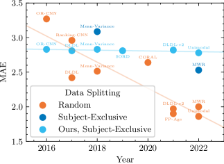
Figure 1: Mean Absolute Error (MAE) $\downarrow$ of age estimation methods on the MORPH dataset, as reported in the existing literature and measured by us, viewed over time. Random splitting remains the prevalent data splitting strategy. The consistent performance improvements over time are attributed in the literature to specialized loss functions for age estimation. Subject-exclusive data splitting is rarely employed. With unified subject-exclusive data splitting and all factors except the loss function fixed, all evaluated methods yield comparable results, failing to achieve the performance gains promised by the random splitting.

2 Critique of Current Evaluation Practices

2.1 Data Splits

Publications focused on age estimation evaluate their methods on several datasets [20, 1, 4, 23, 29, 24, 21]. The most commonly used of these is the MORPH [23] dataset. However, the evaluation procedures between the publications are not unified. For instance, OR-CNN [21] randomly divides the dataset into two parts: 80% for training and 20% for testing. No mention is made of a validation set for model selection. Random splitting (RS) protocol is also used in [19, 28, 3, 12, 13, 5], but the specific data splits differ between studies as they are rarely made public. Since the dataset contains multiple images per person (many captured at the same age), the same individual can be present in both the training and testing sets. This overlap introduces a bias, resulting in overly optimistic evaluation outcomes. The degree of data leakage can vary when using random splitting, making certain data splits more challenging than others. Further, this fundamentally changes the entire setup; rarely will one want to deploy the age estimation system on the people present in the training data. Consequently, comparison of different methods and discerning which method stands out as the most effective based on the published results becomes problematic.

Only some publications [22, 27] recognize this bias introduced by the splitting strategy and address it by implementing subject-exclusive (SE) splitting. This approach ensures that all images of an individual are exclusively in the (i) training (ii) validation (iii) testing part.

To assess how prevalent random splitting (RS) on the MORPH dataset truly is, we conducted a survey of all age estimation papers presented at the CVPR and ICCV since 2013 (see Appendix). We found 16 papers focused on age estimation, of which nine use RS, two use SE, five use specialized splits, and three do not utilize MORPH. We further surveyed other research conferences and journals, namely: IJCAI, BMVC, ACCV, IEEE TIP, Pattern Recognit. Lett., Pattern Anal. Appl., and find eight influential age estimation papers that use MORPH. Of those, seven use RS, and one uses a specialized split.

Altogether, we discover that only $\approx 10\%$ of papers that utilize MORPH use the SE protocol. This finding is concerning, as MORPH [23] is the most popular dataset used to compare age estimation approaches. Other datasets do not provide a reliable benchmark either, as standardized data splits are provided only for two public age estimation datasets: (i) the ChaLearn Looking at People Challenge 2016 (CLAP2016) dataset [1], which is relatively small, consisting of fewer than 8000 images (ii) the Cross-Age Celebrity Dataset (CACD2000) [4], which has noisy training annotations and is not intended for age estimation. Comparing methods using only these datasets is, therefore, not satisfactory either. Other popular datasets, AgeDB dataset [20] and Asian Face Age Dataset (AFAD) [21], also consist of multiple images per person, requiring SE splitting. However, they lack any data splits accepted by the community and often are used with the RS protocol. As such, they suffer from the same issues as MORPH [23].

2.2 Pipeline Components

To fairly compare multiple methods, the same experimental setup should be used for each of them. The current state-of-the-art age estimation approaches follow a common processing pipeline encompassing four key components: (i) data preprocessing (ii) model architecture (iii) the decision layer and the loss function (iv) the specific data for training the model and evaluating its performance. While novel approaches introduce distinct component (iii), they frequently alter multiple components simultaneously, complicating the attribution of perfomance improvements to the claimed modifications.

To compare different loss functions, e.g., [21, 3, 22, 17, 16, 12, 13, 10], the components (i), (ii), and (iv) should be kept constant while varying component (iii), allowing us to isolate the impact of the selected method on the performance. This seems trivial, yet the age estimation community mostly ignores it. Further, many publications hand-wave the other components and do not precisely specify them, making future comparisons meaningless. It’s important to question whether the reported enhancement in a research paper truly stems from the novel loss function it proposes or if it could be attributed to a different modification. We strongly advocate that each component be addressed in isolation and that the experimental setup be precisely described.

Over the past decade, numerous novel age estimation methods have been introduced, promising continuous performance improvements every year. However, motivated by these findings, we raise the question: how reliable are the published age estimation results? In Sec. 3 we aim to establish a proper evaluation protocol and use it in Sec. 4 to the methods [25, 12, 13, 22, 17, 10, 21] reliably. Figure 1 illustrates the contrast between the performance of state-of-the-art methods as reported in their respective studies and the outcomes achieved through the implementation of our proposed evaluation protocol.

3 Evaluation Protocol

We identified two trivial yet persistent issues that prevent a reliable comparison of age estimation methods. In this section, we address the initial challenge concerning consistent data partitioning. We provide clear guidelines for the evaluation protocol to ensure replicable and fair assessments. Specifically, the protocol should establish a reproducible approach for defining the data used in both (i) training and (ii) performance evaluation. When specifying the training data, one needs to state whether the training dataset is the sole source of information, or if the model was pretrained with additional data. Additionally, the evaluation can be subdivided based on the data used for model evaluation into intra-dataset, and cross-dataset results. We describe how to evaluate models in these settings below.

Intra-dataset performance

To evaluate intra-dataset performance, a single dataset is used for both training and evaluation of the age estimation system. In this case one should (i) randomly split the dataset into subject-exclusive training, validation, and test set  (ii) train the model on the training set (iii) measure the model’s performance on the validation set (iv) possibly revert back to step (ii) and train the model again (v) evaluate the model’s performance on the test set (vi) publish the results on the test set along with a detailed description of the system components and the data used. If the dataset consists of limited number of examples, it is possible to create multiple splits of the data into training, validation and test set through step (i). Following this, steps (ii) through (v) are iterated $n$ times, where $n$ is the number of generated splits. It is advisable to present the average test performance along with its standard deviation when reporting the results.

Cross-dataset performance

To evaluate cross-dataset performance, the data split in step (i) of the aforementioned evaluation process is generated from a collection of multiple datasets, ensuring that the complete chosen dataset must be employed entirely for evaluation, effectively constituting the designated test set. The remaning steps of the evaluation procedute remain unaltered.

Regardless of the scenario, whether it is intra-dataset or cross-dataset, each system needs to be evaluated against the test data only once, and the results published. All prior model development and hyperparameter tuning must be based solely on the results on the validation set. Furthermore, it should be indicated whether the training data are the only source of information used for training, or whether the model was pretrained with additional data. In the letter scenario, a detailed description of the additional data and their utilization should also be provided.

4 Comparative Method Analysis

This section applies the evaluation protocol to compare state-of-the-art age estimation methods. We maintain a consistent preprocessing procedure, model architecture, and dataset while selectively altering the decision layer and loss function to incorporate modifications proposed in prominent works such as [25, 12, 13, 22, 17, 10, 21].

4.1 Methodology

Datasets

We evaluate the methods using a total of 7 datasets: AgeDB [20], AFAD [21], CACD2000 [4], CLAP2016 [1], FG-NET [15], MORPH [23], and UTKFace [29]. We also utilize the IMDB-WIKI dataset [24] for pre-training (see the Appendix) with clean labels from Franc and Čech [11].

Data Splits

For the CLAP2016 and CACD2000 datasets, we use the single data split provided by the dataset authors. For the remaining datasets, we create five subject-exclusive (SE) data splits. To generate the split, we partition the dataset such that $60\%$ of the dataset is used for training, $20\%$ for model selection (validation), and $20\%$ for evaluating the model performance (test). Additionally, we ensure that each partition has the same age distribution. Due to its small size, we only use FG-NET for evaluation. We make our data splits public.

Model Architecture & Weight Initialization

We use ResNet-50 [14] as the backbone architecture. We always start the training of the methods from the same initialization. We run the experiments with (i) random initialization (ii) weights pre-trained on ImageNet (TorchVision’s IMAGENET1K_V2) (iii) weights pre-trained on ImageNet and then further pre-trained on IMDB-WIKI (age estimation) with cross-entropy. After the pre-training, the last layer of the model is replaced with a layer specific to the desired method. The models are then fine-tuned on the downstream dataset. It is important to note that for the baseline cross-entropy, we also replace the final layer prior to fine-tuning. This ensures that the experimental setup remains identical to that of the other methods.

Training Details

We utilize the Adam optimizer with the parameters $\beta_{1}=0.9$, $\beta_{2}=0.999$. For pre-training on the IMDB-WIKI dataset, we set the learning rate to ${\alpha=10^{-3}}$ and train the model for a total of 100 epochs. For fine-tuning on the remaining datasets we reduce the learning rate to ${\alpha=10^{-4}}$ and train the model for 50 epochs. We use a batch size of 100. The best model is selected based on the MAE metric computed on the validation set. We utilize two data augmentations during training, (i) horizontal mirroring (ii) cropping out an 80% to 100% portion of the bounding box and resizing it to the model input shape. We acknowledge that with additional hyperparameter tuning, the performance of the models could likely be improved. However, our training parameters are reasonable and serve to compare the methods as if employed out-of-the-box.

Preprocessing

We use the RetinaFace model developed by Deng et al. [8] for face detection and facial landmark detection. We use complete facial coverage, i.e., the images encompass the entire head. We resize the images to a resolution of $256\times 256$ pixels and normalize the pixel values of the images. To this end, we subtract the mean and divide by the standard deviation of the color channels computed over ImageNet [7]. For details of the pre-processing pipeline and the reasoning behind their choice, see the Appendix.

4.2 Results

We use the Mean Absolute Error (MAE) calculated on the test data as the performance measure. To determine whether any method is consistently better than others, we employ the Friedman test and the Nemenyi critical difference test as described by Demšar [6]. The main statistic used in the test is the average ranking ($1$ is best) of a method computed on multiple datasets. Differences in the average ranking are then used to decide whether a method is significantly better than others or whether the improvement is due to randomness (null hypothesis). We use a significance level (p-value) of $\alpha=5\%$.

Intra-Dataset Performance

The intra-dataset results can be seen in Tab. 6, highlighted with a grey background. Using the Friedman test and the Nemenyi test, we can conclude that with pre-training, none of the methods is significantly better than the cross-entropy. In other words, we do not observe any systematic improvement using any of the methods over the standard approach.

When starting from random initialization, we notice that training with the Unimodal loss [17] tends to be unstable. Excluding the Unimodal loss [17] from the evaluation, we apply the Friedman test and the Nemenyi test. The results indicate that OR-CNN [21], DLDL [12], and the Mean-Variance loss [22] demonstrate a significant performance improvement over the cross-entropy. In scenarios with limited data availability, where pre-training is not possible, it is, thus, advisable to utilize one of the aforementioned methods. With the IMDB-WIKI pre-training, the average ranking ($1$ is best) of each method for intra-dataset performance is (i) Cross-Entropy: $3.50$ (ii) OR-CNN [21]: $3.83$ (iii) DLDL [12]: $2.67$ (iv) DLDL-v2 [13]: $3.92$ (v) SORD [10]: $3.00$ (vi) Mean-Variance [22]: $5.92$ (vii) Unimodal [17]: $5.17$ .

Cross-Dataset Generalization

Cross-dataset results, shown in Tab. 6 with white background, were obtained by assessing the performance of models on datasets that were not used for their training. E.g., a model trained on MORPH is evaluated on all of the other datasets. The cross-dataset performance is (unsurprisingly) significantly worse than the intra-dataset performance for all of the methods. Using the Friedman test and the Nemenyi test, we can conclude that there is no significant difference in generalization capability between any of the methods [21, 12, 13, 10, 22, 17] and the cross-entropy, regardless of pre-training. With the IMDB-WIKI pre-training, the average ranking ($1$ is best) of each method for cross-dataset performance is (i) Cross-Entropy: $4.42$ (ii) OR-CNN [21]: $3.35$ (iii) DLDL [12]: $3.62$ (iv) DLDL-v2 [13]: $3.93$ (v) SORD [10]: $3.40$ (vi) Mean-Variance [22]: $4.47$ (vii) Unimodal [17]: $4.81$ .

None of the methods perform well when evaluated on a different dataset than the one they were trained on. The best cross-dataset results are achieved by training on either UTKFace or CLAP2016. The worst performance across databases is observed when models are trained on AFAD or MORPH. This discrepancy can be attributed to UTKFace and CLAP2016 having a broader range of images, which allows them to generalize effectively to other datasets. Conversely, the limited diversity in MORPH or AFAD datasets, such as AFAD mainly comprising images of people of Asian ethnicity and around $80\%$ of MORPH being composed of individuals of African American ethnicity, contributes to the poor knowledge transfer. The significant decrease in the performance of models trained on the MORPH dataset when applied to other age estimation datasets underscores the importance of not relying solely on the MORPH dataset as the benchmark for age estimation. To ensure a reliable evaluation of different methods, it is crucial to incorporate results from alternative datasets as well.

5 Component Analysis

In this section, we analyze the influence of the backbone architecture and the data preparation pipeline on model performance. When altering a system component, we maintain all other components at their defaults, presented as the Cross-Entropy approach in Sec. 4. We use the gained insight to propose a strong baseline age estimation model using the FaRL [30] backbone.

5.1 Model Architecture

Multiple different backbone architectures can be found in the age estimation literature. Among these architectures, VGG16 [13, 28, 27, 22, 17, 10] and ResNet-50 [3, 2, 19] stand out as the most common choice. We evaluate the influence of the architecture choice on the obtained results and present our findings in Tab. 5. We observe that the selection of the model has a more pronounced impact on the performance than the choice of the age estimation method itself.

5.2 Data Preparation Pipeline

Age estimation models require only a specific region of an image, specifically the person’s face, as input, rather than the entire image. However, the influence of this selection process on the model’s performance is not apriori known. Additionally, facial images used for age estimation can differ in terms of scale and resolution since they originate from various sources and as such need to be resized to a uniform resolution. In this section, we examine the impact of the aforementioned data preparation pipeline on the performance of age estimation models.

Facial Alignment

Numerous studies lack an explanation of their facial alignment procedure. Others merely mention the utilization of facial landmarks. To assess whether a standardized alignment is needed for a fair comparison of multiple methods, we adopt three distinct alignment procedures and evaluate their effect on model performance. Firstly, we (i) perform no alignment and employ the bounding box proposed by the facial detection model [8] as the simplest approach. Secondly (ii) we utilize the proposed bounding box but rotate it to horizontally align the eyes. Lastly (iii) we use alignment procedure, which normalizes the rotation, positioning, and scale, and is described in the Appendix. A visual representation of these facial alignment methods is depicted in Fig. 2. The performance of models trained using the various alignment procedures is presented in Tab. 1. When working with pre-aligned datasets like AFAD, we observe that procedure (iii) does not yield significant improvements compared to the simpler variants (i) or (ii). Similar results are obtained on datasets collected under standardized conditions, such as the MORPH dataset. However, when dealing with in-the-wild datasets like AgeDB and CLAP2016, we find that alignment procedure (iii) leads to noticeable improvements over the simpler methods. Interestingly, on the UTKFace dataset, which also contains in-the-wild images, approach (ii) of solely rotating the proposed bounding boxes achieves superior outcomes compared to approach (iii). In summary, the disparities among the various alignment procedures are not substantial. Hence, it can be argued that any facial alignment technique that effectively normalizes the position, rotation, and scale of the faces would yield comparable results.

Facial Coverage

While facial alignment defines the positioning, orientation, and scale of facial landmarks, the extent to which the face is visible in an image also needs to be specified. We refer to this notion as facial coverage. It measures how much of the face is shown in an image and can range from minimal coverage, where only the eyes and mouth are visible, to complete coverage, where the entire head is visible. Determining the optimal compromise between complete facial coverage and minimal coverage is not immediately clear. Complete facial coverage provides a comprehensive view of the face, allowing age estimation algorithms to consider a broader range of facial cues. On the other hand, partial coverage may help reduce overfitting by eliminating irrelevant facial cues and features with high variance. For a visual demonstration of various facial coverage levels, refer to Fig. 3. Surprisingly, the concept of facial coverage has received limited attention in age estimation literature. Consequently, the extent of facial coverage utilized in previous studies can only be inferred from the images presented in those works. For instance, Berg et al. [2] seemingly employ minimal coverage, showing slightly more than just the mouth and eyes. The majority of other works [21, 27, 12, 13, 3, 17] tend to adopt partial coverage, where a significant portion of the face, including the chin and forehead, is visible, but not the entire head. In the works of Pan et al. [22], Rothe et al. [25], and Zhang et al. [28], the entire head is shown.

The performance of models trained with the different coverage levels is presented in Tab. 2. Generally, complete facial coverage, which includes the entire head in the model input, yields the best results across the majority of datasets. However, in cases such as the AFAD dataset or the MORPH dataset, partial coverage performs better. It is important to note that the AFAD dataset contains preprocessed images that do not capture the entire head. Consequently, using complete facial coverage with this dataset results in the presence of black bars and a decrease in the effective pixel resolution of the face. Therefore, it is expected that increased facial coverage would yield inferior results compared to partial coverage on this dataset. The smallest coverage, limited to the facial region up to the eyes and mouth, consistently performs the worst. It can be concluded that with sufficient pixel resolution, the full facial coverage is superior.

Input Resolution

To investigate the influence of input resolution on age estimation, we performed experiments using multiple resolutions on all datasets: specifically, $256\times 256$, $128\times 128$, and $64\times 64$ pixels. The performance of the models trained with different input resolutions is presented in Tab. 3. Our findings indicate that an increase in image resolution consistently results in improved model performance across all datasets. Hence, the best performance was achieved with a resolution of $256\times 256$ pixels. However, it remains uncertain whether further increases in image resolution would yield even more impressive results.

Input Transform

We also examined the input transformation proposed by Lin et al. [18], which involves converting a face image into a tanh-polar representation. This approach has shown great performance in face semantic segmentation. Lin et al. then modified the network for age estimation, reporting impressive results [19]. We explored the potential benefits of applying this transformation for age estimation. However, our findings indicate that the transformation does not improve the results compared to the baseline, as shown in Tab. 4. Therefore, we conclude that the improved age estimation performance observed by Lin et al. [19] does not arise from the use of a different representation, but rather from pre-training on semantic segmentation or their specialized model architecture.

(a) Crop.

(b) Rotation.

(c) Rot., Trans., Scale.

Figure 2: Comparison of different alignment methods using the average face from the FG-NET dataset.

(a) Eyes & Mouth.

(b) Chin & Forehead.

(c) Head.

Figure 3: Comparison of different facial coverage levels using the average face from the FG-NET dataset.

Dataset	Alignment
	Crop	Rotation	Rot. + Trans. + Scale
AgeDB	5.93	5.92	5.84
AFAD	3.12	3.11	3.11
CACD2000	4.01	4.00	4.00
CLAP2016	4.68	4.57	4.49
MORPH	2.81	2.78	2.79
UTKFace	4.49	4.42	4.44

Table 1: MAE $\downarrow$ of ResNet-50 models with different facial alignment. The models were pre-trained on IMDB-WIKI.

Dataset	Facial Coverage
	Eyes & Mouth	Chin & Forehead	Head
AgeDB	6.06	5.84	5.81
AFAD	3.17	3.11	3.14
CACD2000	4.02	4.00	3.96
CLAP2016	5.06	4.49	4.49
MORPH	2.88	2.79	2.81
UTKFace	4.63	4.44	4.38

Table 2: MAE $\downarrow$ of ResNet-50 models with different facial coverages. The models were pre-trained on IMDB-WIKI.

Dataset	Image Resolution
	$64\times 64$	$128\times 128$	$256\times 256$
AgeDB	8.43	6.90	5.81
AFAD	3.36	3.25	3.14
CACD2000	5.01	4.55	3.96
CLAP2016	11.34	5.90	4.49
MORPH	3.33	3.07	2.81
UTKFace	5.83	4.81	4.38

Table 3: MAE $\downarrow$ of ResNet-50 models with different image resolutions. The models were pre-trained on IMDB-WIKI.

Dataset	Transform
	No Transform	RoI Tanh-polar [18]
AgeDB	5.81	5.93
AFAD	3.14	3.15
CACD2000	3.96	4.07
CLAP2016	4.49	4.71
MORPH	2.81	2.80
UTKFace	4.38	4.39

Table 4: MAE $\downarrow$ of ResNet-50 models with different input transformations. The models were pre-trained on IMDB-WIKI.

Backbone	Dataset
	AgeDB	AFAD	CACD2000	CLAP2016	MORPH	UTKFace
ResNet-50	5.81	3.14	3.96	4.49	2.81	4.38
EfficientNet-B4	5.76	3.20	4.00	4.06	2.87	4.23
ViT-B-16	9.07	4.04	6.22	8.55	4.35	6.88
VGG-16	6.02	3.22	3.92	4.65	2.88	4.64

Table 5: Intra-dataset MAE $\downarrow$ with different backbone architectures. The models were pre-trained on IMDB-WIKI [24].

5.3 FaRL Backbone

In our investigation, we observed that adjustments to the decision layer and loss function, referred to as component (iii) in Sec. 2.2, have minimal impact on the final model performance. Conversely, substantial performance disparities arise when modifying components (i), (ii), or (iv). Notably, the model architecture and pretraining data emerge as the most influential factors. Based on this insight, we opt against creating a specialized loss function to enhance the age estimation system. Instead, we leverage the FaRL backbone by Zheng et al. [30], utilizing a ViT-B-16 [9] model. The FaRL model is trained through a combination of (i) contrastive loss on image-text pairs and (ii) prediction of masked image patches. Training takes place on an extensive collection of facial images from the image-text pair LAION dataset [26]. We retain the features extracted by FaRL without altering the model’s weights. We employ a simple multilayer perceptron (MLP) over the FaRL-extracted features, consisting of 2 layers with 512 neurons each, followed by ReLU activation. Cross-entropy serves as the chosen loss function. For each downstream dataset, we pretrain the MLP on IMDB-WIKI or initialize it to random weights. We choose the preferred option based on validation loss on the downstream dataset. As previously, we replace the final layer before fine-tuning on downstream datasets.

Remarkably, this straightforward modification outperformed all other models on AgeDB, CLAP2016, and UTKFace datasets. It also achieved superior results on AFAD, matched the performance of other models on CACD2000, but demonstrated worse performance on MORPH. Overall, applying the Friedman and Nemenyi tests revealed statistically significant improvements of this model over others in both intra-dataset and cross-dataset evaluations, see Tab. 6. We attribute the poor performance of FaRL on MORPH to the fact that the distributions of images in LAION [26] and MORPH [23] are vastly different. As we do not finetune the feature representation of FaRL [30], it is possible that the representation learned on LAION is superior on the other datasets but deficient on MORPH.

We do not assert this model to be the ultimate solution, but the results achieved with the FaRL backbone offer a robust and straightforward baseline for a comparison with future age estimation systems.

6 Discussion and Conclusions

In this paper, we aimed to establish a fair comparison framework for evaluating various approaches for age estimation. We conducted a comprehensive analysis on seven different datasets, namely AgeDB [20], AFAD [21], CACD2000 [4], CLAP2016 [1], FG-NET [15], MORPH [23], and UTKFace [29], comparing the models based on their Mean Absolute Error (MAE). To determine if any method outperformed the others, we employed the Friedman test and the Nemenyi critical difference test. When pre-training the models on a large dataset, we did not observe any statistically significant improvement by using the specialized loss functions designed for age estimation. With random model initialization, we observed some improvement over the baseline cross-entropy on small datasets. Specifically, the Mean-Variance loss [22], OR-CNN [21], and DLDL [12] demonstrated better performance. These improvements can be attributed to the regularization provided by these methods.

Previously published results reported continuous performance improvements over time (as depicted in Fig. 1). However, our findings challenge these claims. We argue that the reported improvements can be attributed to either the random data splitting strategy or hyperparameter tuning to achieve the best test set performance. Furthermore, our analysis of the data preparation pipeline (see Appendix for details) revealed that factors such as the extent of facial coverage, input resolution, and the facial alignment procedure exert a more significant impact on the achieved results compared to the choice of the age estimation method itself. Guided by this insight, we proposed to use the FaRL [30] model as a backbone for age estimation and demonstrated its effectiveness. In summary:

• We show that existing evaluation practices in age estimation do not provide a consistent comparison of the state-of-the-art methods. We define a proper evaluation protocol which addresses the issue.

• We show that improvements in age estimation results over recent years can not be attributed to the specialized loss functions introduced in [21, 12, 13, 10, 22, 17], as is claimed in the published literature.

• Using the insight gained from analyzing different components of the age estimation pipeline, we construct a prediction model with the FaRL [30] backbone and demonstrate its effectiveness.

• To facilitate reproducibility and simple future comparisons, we have made our implementation framework and the exact data splits publicly available. github.com/anonymous.

Training Dataset Evaluation Dataset AgeDB AFAD CACD2000 CLAP2016 FG-NET MORPH UTKFace IMDB Imag. Rand. IMDB Imag. Rand. IMDB Imag. Rand. IMDB Imag. Rand. IMDB Imag. Rand. IMDB Imag. Rand. IMDB Imag. Rand. AgeDB Cross-Entropy 5.81 7.20 7.65 7.83 12.61 14.70 5.90 8.10 8.73 6.83 10.86 12.41 10.82 16.27 18.87 4.83 6.74 6.93 8.45 11.88 11.82 Regression 6.23 6.54 7.60 8.05 12.13 14.19 6.76 7.56 8.74 8.32 9.95 12.32 10.56 13.83 18.00 5.64 6.66 6.94 9.42 10.42 12.14 OR-CNN [21] 5.78 6.51 7.52 7.47 11.86 13.80 6.05 7.71 8.55 6.64 10.18 11.74 9.74 13.82 17.40 4.73 6.61 7.05 8.20 10.75 11.41 DLDL [12] 5.80 6.95 7.46 7.81 1.85 14.92 5.99 7.96 8.52 6.51 10.84 11.48 9.23 15.63 16.95 4.74 6.34 6.82 7.97 11.87 11.24 DLDL-v2 [13] 5.80 6.87 7.58 7.61 12.98 16.19 5.91 8.15 8.61 6.48 10.88 12.50 9.91 15.36 19.01 4.92 7.53 7.20 7.97 11.61 12.30 SORD [10] 5.81 6.93 7.58 7.81 12.80 15.42 5.96 7.90 8.77 6.61 10.37 12.22 9.72 14.76 17.85 4.76 6.58 7.14 8.12 11.53 11.60 Mean-Var. [22] 5.85 6.69 7.33 7.26 12.40 14.35 6.00 7.89 8.35 6.70 10.50 11.90 10.55 14.32 17.43 4.99 6.87 7.33 8.25 10.77 11.64 Unimodal [17] 5.90 7.11 15.49 8.37 13.11 20.87 6.22 8.24 16.11 6.73 11.14 21.31 10.15 16.13 32.77 4.84 6.78 17.42 8.23 11.86 23.09 FaRL + MLP 5.64 - - 7.82 - - 7.41 - - 9.32 - - 9.15 - - 4.73 - - 9.92 - - AFAD Cross-Entropy 15.70 17.31 18.05 3.14 3.17 3.32 9.54 11.18 11.21 8.96 10.23 10.32 10.92 11.38 11.96 6.80 6.83 8.19 12.10 13.07 13.29 Regression 13.67 15.91 17.21 3.17 3.16 3.30 8.72 10.51 10.72 8.33 9.91 10.02 11.20 11.89 12.35 6.27 7.34 7.99 11.23 12.83 12.96 OR-CNN [21] 12.08 15.65 16.72 3.16 3.17 3.28 8.87 11.05 10.89 7.85 9.73 9.92 10.63 11.94 12.58 6.68 6.85 7.81 10.50 12.43 12.74 DLDL [12] 14.12 15.70 17.21 3.14 3.16 3.25 9.40 10.70 11.06 8.68 9.54 9.98 11.31 11.64 12.07 7.04 6.75 7.82 11.52 12.43 12.82 DLDL-v2 [13] 13.90 16.33 17.78 3.15 3.17 3.28 9.46 10.68 11.02 8.60 9.76 10.32 10.83 11.81 12.64 6.92 6.79 7.94 11.29 12.61 13.18 SORD [10] 14.30 16.08 17.49 3.14 3.15 3.24 9.45 10.70 11.09 8.64 9.79 10.10 11.21 11.63 12.19 6.87 6.82 7.93 11.59 12.79 13.10 Mean-Var. [22] 12.54 15.07 16.68 3.16 3.16 3.26 8.98 10.33 10.75 7.93 9.33 9.78 10.96 12.24 12.43 6.61 6.76 7.88 10.57 12.00 12.62 Unimodal [17] 13.99 15.89 20.97 3.20 3.24 9.30 9.23 10.68 14.56 8.64 9.79 14.51 11.31 11.83 18.29 7.07 7.32 12.53 11.26 12.33 17.47 FaRL + MLP 16.41 - - 3.12 - - 10.95 - - 8.57 - - 12.24 - - 6.62 - - 11.64 - - CACD2000 Cross-Entropy 9.66 11.84 10.60 10.70 8.50 13.08 3.96 4.59 4.89 8.42 8.64 10.51 17.45 23.64 20.86 7.21 12.20 10.39 11.16 11.38 12.61 Regression 10.91 10.44 10.76 10.23 7.23 11.66 4.06 4.52 4.83 8.84 7.75 9.98 17.55 19.50 19.60 8.61 8.81 11.79 11.34 10.38 11.78 OR-CNN [21] 10.43 11.02 11.85 9.66 9.48 12.17 4.01 4.60 4.74 8.57 8.85 10.29 18.47 24.32 20.85 7.52 10.04 11.05 11.17 12.30 12.27 DLDL [12] 9.84 10.79 11.28 10.09 9.30 13.20 3.96 4.42 4.76 8.39 8.49 9.99 18.38 18.99 21.52 7.27 9.16 11.01 11.19 11.94 12.27 DLDL-v2 [13] 9.90 12.31 11.20 8.03 11.50 11.51 3.96 4.57 4.69 7.67 8.88 9.43 18.11 22.89 19.02 7.20 13.46 9.73 10.52 12.32 11.47 SORD [10] 9.77 10.90 11.04 10.35 9.55 11.95 3.96 4.42 4.70 8.38 8.51 9.89 18.05 20.84 21.73 7.23 8.98 11.59 11.18 12.06 12.22 Mean-Var. [22] 10.81 11.42 10.83 9.71 10.82 11.49 4.07 4.60 4.78 8.88 9.20 10.08 20.48 22.68 20.14 8.14 12.59 11.72 11.74 12.29 12.23 Unimodal [17] 10.46 11.04 46.26 10.63 9.85 25.74 4.10 4.73 37.41 9.19 8.92 30.96 19.37 19.75 15.84 8.94 11.64 32.63 11.89 11.75 32.98 FaRL + MLP 11.32 - - 9.08 - - 3.96 - - 8.57 - - 19.63 - - 6.56 - - 11.27 - - CLAP2016 Cross-Entropy 7.35 10.15 12.26 5.41 7.03 5.34 6.65 8.11 9.11 4.49 5.96 8.73 5.92 9.28 12.02 4.96 6.61 6.90 5.74 7.21 8.58 Regression 7.51 8.52 11.74 6.07 5.19 5.95 6.86 7.24 9.45 4.65 4.77 7.89 4.85 6.31 10.14 5.09 5.49 8.83 6.02 5.93 8.66 OR-CNN [21] 6.83 8.74 11.24 5.83 5.92 5.44 6.73 7.25 8.65 4.13 4.60 7.38 5.09 6.47 9.22 4.92 5.78 6.52 5.43 5.95 7.68 DLDL [12] 7.20 9.33 11.39 5.57 6.90 5.85 6.85 7.64 9.26 4.18 5.10 7.39 5.26 7.44 9.18 4.89 5.92 6.52 5.51 6.37 7.87 DLDL-v2 [13] 7.14 9.42 12.36 5.47 5.95 6.45 6.69 7.99 9.34 4.23 4.87 8.52 5.22 7.04 8.75 4.85 6.04 7.29 5.53 6.12 8.23 SORD [10] 7.19 9.60 12.16 5.47 7.74 6.62 6.63 8.09 9.66 4.27 5.34 7.81 5.59 7.77 7.62 4.92 6.01 6.62 5.48 6.46 8.08 Mean-Var. [22] 7.08 9.16 12.58 5.18 6.30 5.38 6.64 7.37 9.94 4.28 4.87 7.95 5.45 6.69 11.14 4.96 7.38 7.49 5.52 6.16 8.65 Unimodal [17] 7.01 9.77 20.71 5.58 6.10 5.54 6.47 8.20 13.08 4.17 5.39 13.83 5.13 6.39 15.13 4.80 6.05 10.02 5.44 6.67 15.27 FaRL + MLP 7.50 - - 4.34 - - 6.57 - - 3.38 - - 4.95 - - 4.47 - - 4.85 - - MORPH Cross-Entropy 9.66 11.73 12.63 6.69 7.78 10.36 8.53 10.83 10.11 6.90 8.96 10.64 9.45 11.96 15.38 2.81 2.96 3.01 8.97 10.81 11.92 Regression 10.48 12.99 12.56 6.60 6.65 10.66 9.82 11.47 9.68 7.83 9.27 10.67 9.24 10.13 16.69 2.83 2.74 2.97 9.40 10.97 12.06 OR-CNN [21] 9.35 11.65 12.82 6.78 7.78 11.81 8.39 11.34 10.23 6.84 8.73 11.05 9.58 11.09 17.47 2.83 2.85 2.99 8.82 10.37 12.06 DLDL [12] 9.41 12.00 12.66 6.58 7.78 11.76 8.58 11.92 10.10 6.85 9.26 11.15 9.44 11.43 16.94 2.81 2.92 2.98 8.80 10.81 12.46 DLDL-v2 [13] 9.79 11.49 12.68 6.60 8.22 12.45 8.79 10.98 9.81 6.98 8.98 11.22 9.52 11.63 17.57 2.82 2.93 3.00 8.97 10.70 12.47 SORD [10] 9.48 11.84 12.73 6.54 7.91 11.19 8.73 11.18 10.13 6.84 8.99 10.72 9.34 11.08 15.90 2.81 2.91 2.99 8.83 10.85 11.97 Mean-Var. [22] 9.70 11.62 12.93 6.68 7.81 10.41 8.65 10.59 10.11 7.03 8.80 10.56 9.51 11.45 15.81 2.83 2.89 2.95 8.94 10.59 11.95 Unimodal [17] 9.93 12.31 17.44 6.63 7.04 8.18 8.68 10.11 12.03 7.19 8.95 12.38 9.80 12.17 17.83 2.78 2.90 8.66 9.07 10.75 15.45 FaRL + MLP 8.40 - - 4.67 - - 7.45 - - 6.21 - - 9.28 - - 3.04 - - 8.93 - - UTKFace Cross-Entropy 6.61 8.88 9.58 5.51 6.42 6.75 6.56 9.10 8.98 4.82 7.34 7.50 4.78 6.62 7.64 5.09 6.61 7.35 4.38 4.75 5.32 Regression 7.01 7.79 8.83 5.96 6.26 6.43 6.77 7.87 8.61 5.24 5.93 6.67 4.41 5.07 7.27 5.41 5.95 6.71 4.72 4.53 5.34 OR-CNN [21] 6.71 8.29 8.75 5.56 6.74 6.52 6.61 8.89 8.37 4.95 6.79 6.70 4.54 5.71 6.55 5.26 6.07 6.76 4.40 4.43 5.15 DLDL [12] 6.65 8.60 9.00 5.42 6.68 6.19 6.52 9.01 8.84 4.81 7.19 7.46 4.85 5.87 7.28 5.16 6.25 7.03 4.39 4.66 5.30 DLDL-v2 [13] 6.79 8.43 8.91 5.45 6.65 5.82 6.61 9.39 8.50 4.98 7.27 6.85 4.79 5.93 7.44 5.46 6.24 6.79 4.42 4.60 5.19 SORD [10] 6.61 8.96 9.11 5.42 7.18 6.32 6.52 9.42 8.69 4.82 7.87 7.18 4.83 6.15 7.55 5.14 6.36 7.28 4.36 4.68 5.25 Mean-Var. [22] 6.79 8.36 8.53 5.41 6.54 6.32 6.55 8.55 8.32 5.04 6.81 6.32 5.05 6.30 6.90 5.37 6.15 6.39 4.42 4.57 5.05 Unimodal [17] 6.68 8.66 22.42 5.35 7.68 16.64 6.58 9.28 17.17 4.86 7.60 18.83 4.55 6.25 22.98 5.22 5.96 16.44 4.47 4.78 21.01 FaRL + MLP 7.16 - - 4.69 - - 6.93 - - 4.02 - - 5.07 - - 4.76 - - 3.87 - -

Table 6: Intra-dataset and cross-dataset Mean Absolute Error (MAE) $\downarrow$ of ResNet-50 models. Results marked as Initialization: IMDB are of models that are initialized to ImageNet weights, then trained with Cross-Entropy on IMDB-WIKI [24] and then finetuned on the downstream dataset. Imag. signifies initialization to weights pre-trained on ImageNet. Rand. denotes random initialization.

References

- [1] E. Agustsson, R. Timofte, S. Escalera, X. Baro, I. Guyon, and R. Rothe. Apparent and real age estimation in still images with deep residual regressors on appa-real database. In 12th IEEE International Conference and Workshops on Automatic Face and Gesture Recognition (FG), 2017. IEEE, 2017.
- [2] A. Berg, M. Oskarsson, and M. O’Connor. Deep ordinal regression with label diversity. In 2020 25th International Conference on Pattern Recognition (ICPR), pages 2740–2747, Los Alamitos, CA, USA, jan 2021. IEEE Computer Society.
- [3] Wenzhi Cao, Vahid Mirjalili, and Sebastian Raschka. Rank consistent ordinal regression for neural networks with application to age estimation. Pattern Recognition Letters, 140:325–331, 2020.
- [4] Bor-Chun Chen, Chu-Song Chen, and Winston H. Hsu. Cross-age reference coding for age-invariant face recognition and retrieval. In David Fleet, Tomas Pajdla, Bernt Schiele, and Tinne Tuytelaars, editors, Computer Vision – ECCV 2014, pages 768–783, Cham, 2014. Springer International Publishing.
- [5] Shixing Chen, Caojin Zhang, Ming Dong, Jialiang Le, and Mike Rao. Using ranking-cnn for age estimation. In 2017 IEEE Conference on Computer Vision and Pattern Recognition (CVPR), pages 742–751, 2017.
- [6] Janez Demšar. Statistical comparisons of classifiers over multiple data sets. The Journal of Machine learning research, 7:1–30, 2006.
- [7] Jia Deng, Wei Dong, Richard Socher, Li-Jia Li, Kai Li, and Li Fei-Fei. Imagenet: A large-scale hierarchical image database. In 2009 IEEE Conference on Computer Vision and Pattern Recognition, pages 248–255, 2009.
- [8] Jiankang Deng, Jia Guo, Evangelos Ververas, Irene Kotsia, and Stefanos Zafeiriou. Retinaface: Single-shot multi-level face localisation in the wild. In Proceedings of the IEEE/CVF Conference on Computer Vision and Pattern Recognition, pages 5203–5212, 2020.
- [9] Alexey Dosovitskiy, Lucas Beyer, Alexander Kolesnikov, Dirk Weissenborn, Xiaohua Zhai, Thomas Unterthiner, Mostafa Dehghani, Matthias Minderer, Georg Heigold, Sylvain Gelly, Jakob Uszkoreit, and Neil Houlsby. An image is worth 16x16 words: Transformers for image recognition at scale. In 9th International Conference on Learning Representations, ICLR 2021, Virtual Event, Austria, May 3-7, 2021. OpenReview.net, 2021.
- [10] Raúl Díaz and Amit Marathe. Soft labels for ordinal regression. In 2019 IEEE/CVF Conference on Computer Vision and Pattern Recognition (CVPR), pages 4733–4742, 2019.
- [11] Vojtech Franc and Jan Cech. Learning cnns from weakly annotated facial images. Image and Vision Computing, 2018.
- [12] Bin-Bin Gao, Chao Xing, Chen-Wei Xie, Jianxin Wu, and Xin Geng. Deep label distribution learning with label ambiguity. IEEE Transactions on Image Processing, 26(6):2825–2838, 2017.
- [13] Bin-Bin Gao, Hong-Yu Zhou, Jianxin Wu, and Xin Geng. Age estimation using expectation of label distribution learning. In Proceedings of the Twenty-Seventh International Joint Conference on Artificial Intelligence, IJCAI-18, pages 712–718. International Joint Conferences on Artificial Intelligence Organization, 7 2018.
- [14] Kaiming He, Xiangyu Zhang, Shaoqing Ren, and Jian Sun. Deep residual learning for image recognition. In 2016 IEEE Conference on Computer Vision and Pattern Recognition (CVPR), pages 770–778, 2016.
- [15] A. Lanitis, C.J. Taylor, and T.F. Cootes. Toward automatic simulation of aging effects on face images. IEEE Transactions on Pattern Analysis and Machine Intelligence, 24(4):442–455, 2002.
- [16] Ling Li and Hsuan-Tien Lin. Ordinal regression by extended binary classification. In Advances in Neural Information Processing Systems, page 865 – 872, 2007. Cited by: 195.
- [17] Qiang Li, Jingjing Wang, Zhaoliang Yao, Yachun Li, Pengju Yang, Jingwei Yan, Chunmao Wang, and Shiliang Pu. Unimodal-concentrated loss: Fully adaptive label distribution learning for ordinal regression. In Proceedings of the IEEE/CVF Conference on Computer Vision and Pattern Recognition (CVPR), pages 20513–20522, June 2022.
- [18] Yiming Lin, Jie Shen, Yujiang Wang, and Maja Pantic. Roi tanh-polar transformer network for face parsing in the wild. Image and Vision Computing, 112, 2021.
- [19] Yiming Lin, Jie Shen, Yujiang Wang, and Maja Pantic. Fp-age: Leveraging face parsing attention for facial age estimation in the wild. IEEE Transactions on Image Processing, 2022.
- [20] Stylianos Moschoglou, Athanasios Papaioannou, Christos Sagonas, Jiankang Deng, Irene Kotsia, and Stefanos Zafeiriou. Agedb: the first manually collected, in-the-wild age database. In Proceedings of the IEEE Conference on Computer Vision and Pattern Recognition Workshop, volume 2, 2017.
- [21] Zhenxing Niu, Mo Zhou, Le Wang, Xinbo Gao, and Gang Hua. Ordinal regression with multiple output cnn for age estimation. In 2016 IEEE Conference on Computer Vision and Pattern Recognition (CVPR), pages 4920–4928, 2016.
- [22] Hongyu Pan, Hu Han, Shiguang Shan, and Xilin Chen. Mean-variance loss for deep age estimation from a face. In 2018 IEEE/CVF Conference on Computer Vision and Pattern Recognition, pages 5285–5294, 2018.
- [23] K. Ricanek and T. Tesafaye. Morph: a longitudinal image database of normal adult age-progression. In 7th International Conference on Automatic Face and Gesture Recognition (FGR06), pages 341–345, 2006.
- [24] Rasmus Rothe, Radu Timofte, and Luc Van Gool. Deep expectation of real and apparent age from a single image without facial landmarks. International Journal of Computer Vision, 126(2-4):144–157, 2018.
- [25] Rasmus Rothe, Radu Timofte, and Luc Van Gool. Dex: Deep expectation of apparent age from a single image. In 2015 IEEE International Conference on Computer Vision Workshop (ICCVW), pages 252–257, 2015.
- [26] Christoph Schuhmann, Romain Beaumont, Richard Vencu, Cade W Gordon, Ross Wightman, Mehdi Cherti, Theo Coombes, Aarush Katta, Clayton Mullis, Mitchell Wortsman, Patrick Schramowski, Srivatsa R Kundurthy, Katherine Crowson, Ludwig Schmidt, Robert Kaczmarczyk, and Jenia Jitsev. LAION-5b: An open large-scale dataset for training next generation image-text models. In Thirty-sixth Conference on Neural Information Processing Systems Datasets and Benchmarks Track, 2022.
- [27] Nyeong-Ho Shin, Seon-Ho Lee, and Chang-Su Kim. Moving window regression: A novel approach to ordinal regression. In Proceedings of the IEEE/CVF Conference on Computer Vision and Pattern Recognition (CVPR), pages 18760–18769, June 2022.
- [28] Yunxuan Zhang, Li Liu, Cheng Li, and Chen-Change Loy. Quantifying facial age by posterior of age comparisons. In Gabriel Brostow Tae-Kyun Kim, Stefanos Zafeiriou and Krystian Mikolajczyk, editors, Proceedings of the British Machine Vision Conference (BMVC), pages 108.1–108.12. BMVA Press, September 2017.
- [29] Zhifei Zhang, Yang Song, and Hairong Qi. Age progression/regression by conditional adversarial autoencoder. In IEEE Conference on Computer Vision and Pattern Recognition (CVPR). IEEE, 2017.
- [30] Yinglin Zheng, Hao Yang, Ting Zhang, Jianmin Bao, Dongdong Chen, Yangyu Huang, Lu Yuan, Dong Chen, Ming Zeng, and Fang Wen. General facial representation learning in a visual-linguistic manner. In Proceedings of the IEEE/CVF Conference on Computer Vision and Pattern Recognition (CVPR), pages 18697–18709, June 2022.