Manifold Filter-Combine Networks

Abstract

We introduce a class of manifold neural networks (MNNs) that we call Manifold Filter-Combine Networks (MFCNs), which aims to further our understanding of MNNs, analogous to how the aggregate-combine framework helps with the understanding of graph neural networks (GNNs). This class includes a wide variety of subclasses that can be thought of as the manifold analog of various popular GNNs. We then consider a method, based on building a data-driven graph, for implementing such networks when one does not have global knowledge of the manifold, but merely has access to finitely many points sampled from some probability distribution on the manifold. We provide sufficient conditions for the network to provably converge to its continuum limit as the number of sample points tends to infinity. Unlike previous work (which focused on specific graph constructions and assumed that the data was drawn from the uniform distribution), our rate of convergence does not directly depend on the number of filters used. Moreover, it exhibits linear dependence on the depth of the network rather than the exponential dependence obtained previously. Additionally, we provide several examples of interesting subclasses of MFCNs and of the rates of convergence that are obtained under specific graph constructions.

68T07, 53Z50, 65T99 58J50

1 Introduction

Geometric deep learning [7, 6] is an emerging field that aims to extend the success of deep learning from data such as images, with a regular grid-like structure, to more irregular domains such as graphs and manifolds. As part of the rise of geometric deep learning, graph neural networks (GNNs) have rapidly emerged as an extremely active area of research in data science [56, 52] and are also used in industrial applications such as Google Maps[18] and Amazon’s product recommender system[42]. However, there has been much less work on the development of Manifold Neural Networks (MNNs) and much of the existing literature focuses on two-dimensional surfaces embedded in three-dimensional space [30, 5, 31, 39]. In this paper, we consider the more general setting of a compact, connected, $d$-dimensional Riemannian manifold $\mathcal{M}$ embedded in $D$-dimensional space.

One of the principal challenges in extending deep learning to graphs and manifolds is developing a proper notion of convolution, which is non-trivial because there is no natural notion of translation. In the graph setting, a popular family of solutions, known as spectral methods, define convolution via the eigendecomposition of the graph Laplacian (or another suitable matrix). A limitation of this method is that explicitly computing eigendecompositions is expensive for large graphs. To overcome this obstacle, spectral graph neural networks such as ChebNet [17] and CayleyNet [28] define convolution in terms of polynomials of the graph Laplacian $\mathbf{L}=\mathbf{D}-\mathbf{A}$. This leads to filters of the form $h(\mathbf{L})\mathbf{x}$ where $h$ is a polynomial and $\mathbf{x}$ is a signal defined on the vertices of the graph.

With this notion of convolution, one may consider networks with layerwise update rules of the form:

(1) $$\mathbf{x}^{(\ell+1)}=\sigma\left(h^{(\ell)}(\mathbf{L})\mathbf{x}^{(\ell)}\right),$$

where $\sigma$ is a pointwise, nonlinear activation function. If one is given multiple initial graph signals $\mathbf{x}_{1},\ldots,\mathbf{x}_{C}$ organized into a data matrix $\mathbf{X}=(\mathbf{x}_{1},\ldots,\mathbf{x}_{C})$ and uses multiple filters in each layer, then the layerwise update rule can be extended to

(2) $$\mathbf{x}^{(\ell+1)}_{k}=\sigma\left(\sum_{j=1}^{C}h^{(\ell)}_{j,k}(\mathbf{L})\mathbf{x}^{(\ell)}_{j}\right).$$

If one assumes that each filter $h^{\ell}_{j,k}$ belongs to a parameterized family of functions such as Chebyshev polynomials, one could then attempt to learn the optimal parameters from training data.

Inspired by this approach, Wang, Ruiz, and Ribeiro [45, 46] have introduced manifold neural networks with layerwise update rules similar to (2). In particular, they assume that they are given $C$ functions $f_{1},\ldots,f_{C}:\mathcal{M}:\rightarrow\mathbb{R}$ and utilize a layerwise update rule of

(3) $$f^{(\ell+1)}_{k}=\sigma\left(\sum_{j=1}^{C}h^{(\ell)}_{j,k}(\mathcal{L}_{\text{LB}})f^{(\ell)}_{j}\right),$$

where $\mathcal{L}_{\text{LB}}=-\text{div}\circ\nabla$ is the Laplace-Beltrami operator, the natural analog of the graph Laplacian in the manifold setting. They then provide an analysis of the stability of such networks to absolute and relative perturbations of the Laplace-Beltrami operator.

However, many popular graph neural networks take an approach different from (2). Rather than using multiple learnable filters for each input channel and then summing across channels, they instead filter each graph signal with a pre-designed operator (or operators) and then learn relationships between the filtered input signals. For example, the Graph Convolutional Network (GCN) [26] performs a predesigned aggregation

$$\mathbf{X}\rightarrow\widehat{\mathbf{A}}\mathbf{X}$$

where $\widehat{\mathbf{A}}=(\mathbf{D}+\mathbf{I})^{-1/2}(\mathbf{A}+\mathbf{I})(\mathbf{D}+\mathbf{I})^{-1/2}$ and utilizes a right-multiplication by a trainable weight matrix $\mathbf{\Theta}$ to learn relationships between the channels. This leads to the layerwise update rule

(4) $$\mathbf{X}^{(\ell+1)}=\sigma(\widehat{\mathbf{A}}\mathbf{X}^{(\ell)}\Theta^{(\ell)}),$$

where $\sigma$ is as in (1). This raises an intriguing question:

Question 1.1.

How should manifold neural networks be designed? Should they follow the lead of (2) and (3) and utilize multiple learnable filters for each input channel with a predesigned summation over channels or should they utilize predesigned filtering operations and incorporate learning via cross-feature operations analogous to (4)?

It is likely that the answer to this question will vary depending on the dataset and the task of interest. Networks with multiple learnable filters for each channel are more general and will have greater expressive power. On the other hand, networks that, for example, use a common (either learnable or designed) filter bank shared across all channels are a more constrained family of networks. This constraint imposes a certain structure on the network and reduces the number of trainable parameters, which may provide a useful inductive bias in certain settings and may be particularly useful in low-data environments.

Another critical challenge in the development of manifold neural networks is that in many applications one does not have global knowledge of the manifold. Instead, one is given a collection of points $\{x_{j}\}_{j=1}^{n}$ in some high-dimensional Euclidean space $\mathbb{R}^{D}$ and makes the modeling assumption that the points $x_{j}$ lie on some $d$-dimensional manifold for $d\ll D$. This assumption, known as the manifold hypothesis, is frequently used in the analysis of biomedical data arising from, e.g., single-cell imaging [32, 41, 1]. This leads us to the following question:

Question 1.2.

How can one implement a manifold neural network when one does not have global knowledge of the manifold but only has access to finitely many sample points?

In order to help answer this question, several works such as [13, 47, 48, 49] have used an approach based on Laplacian eigenmaps [2] (see also [15]) where one builds a data-driven graph $\mathbf{G}_{n}$ such that the eigenvectors and eigenvalues of the graph Laplacian approximate the eigenfunctions and eigenvalues of the Laplace-Beltrami Operator. They show that if the graph is constructed properly, then a graph neural network of the form (2) will converge to a continuum limit of the form (3) as the number of sample points, $n$, tends to infinity. However, these results are limited in the sense that (i) they assume specific graph constructions (ii) their rates of convergence depend exponentially on the depth of the network, (iii) they assume that points $x_{j}$ are sampled uniformly from the manifold.

1.1 Contributions

In this work, we introduce a new framework for understanding MNNs that we call Manifold Filter-Combine Networks. The manifold filter-combine paradigm is meant to parallel the aggregate-combine framework commonly considered in the GNN literature (see, e.g., [54]) and naturally leads one to consider many interesting classes of MNNs which may be thought of as the manifold counterparts of various popular GNNs. We then provide sufficient conditions for such networks to converge to a continuum limit as the number of sample points, $n$, tends to infinity. We note that unlike previous work on the convergence of MNNs, our results may be applied to settings where the data points are generated from a non-uniform probability distribution which greatly increases the applicability of our theory to real-world data.

More specifically, the contributions of this work are:

1. We introduce Manifold Filter-Combine Networks as a novel framework for understanding MNNs. This framework readily leads one to many interesting classes of MNNs such as the manifold equivalent of Kipf and Welling’s GCN [25], learnable variations of the manifold scattering transform [36, 12], and many others.

2. In Theorem 2.2, we provide sufficient conditions for the individual filters used in an MNN to provably converge to a continuum limit as $n\rightarrow\infty$ if the filtering is done via a spectral approach. Here the rate of convergence depends on the rates at which the eigenvectors/eigenvalues of the graph Laplacian approximate the eigenfunctions/eigenvalues of the continuum Laplacian as well as the rate at which discrete inner products approximate continuum inner products. Notably, unlike previous results on the convergence of spectral filters and MNNs, Theorem 2.2 does not assume that the data points are sampled uniformly from the manifold.

3. In Theorem 3.7, we prove that if the individual filters converge as $n\rightarrow\infty$, then so does the entire MNN. The rate of convergence will depend on (i) the rate of convergence of the individual filters; (ii) the weights used in the network; (iii) the depth of the network. Importantly, we note that our dependence on the depth of the network is linear, rather than the exponential dependence obtained in previous work. Additionally, our rate does not directly depend on the number of filters used per layer. We also note that Theorem 3.7 does not assume that the filters have any particular form. Therefore, if one were to prove results analogous to Theorem 2.2 for non-spectral filters, then Theorem 3.7 would immediately imply the convergence of networks constructed from those filters.

4. We then provide several corollaries to Theorem 3.7, which give concrete examples of our results in special cases of interest in Corollaries 3.8, 3.9, 3.10, and 3.11. These results may be summarized as follows:

   • If the filters are implemented spectrally, then the discretization error of the entire MFCN tends to zero at a rate depending on how fast the eigenvalues/eigenvectors of the Laplacian corresponding to the data-driven graph $\mathbf{G}_{n}$ converge to the eigenvalues/eigenfunctions of the continuum Laplacian and how fast discrete inner products converge to continuum inner products.

   • If $\mathbf{G}_{n}$ is constructed via a Gaussian kernel and the filters are implemented spectrally, then (up to log factors) the discretization error is $\mathcal{O}(n^{-2/(d+6)})$.

   • If $\mathbf{G}_{n}$ is constructed via a $k$-NN graph or an $\epsilon$-graph and the filters are implemented spectrally, then (up to log factors) the discretization error is $\mathcal{O}(n^{-1/(d+4)})$.

1.2 Notation

We let $\mathcal{M}$ be a compact, connected, $d$-dimensional Riemannian manifold and let $\mu$ be a probability distribution on $\mathcal{M}$ with density $\rho$. We let $\mathbf{L}^{2}(\mathcal{M})$ denote the set of functions that are square integrable with respect to $\mu$ and $\mathcal{C}(\mathcal{M})$ denote the set of continuous functions on $\mathcal{M}$. We let $\mathcal{L}_{\rho}$ denote the differential operator which is to be thought of as a weighted Laplacian and let $\{\phi_{i}\}_{i=1}^{\infty}$ denote an orthonormal basis of eigenfunctions $\mathcal{L}_{\rho}\phi_{i}=\lambda_{i}\phi_{i}.$ We will use these eigenfunctions to define Fourier coefficients denoted by $\widehat{f}(i).$

In much of our analysis, we will assume that $\mathcal{M}$ is unknown and that we only have access to a function $f\in\mathcal{C}(\mathcal{M})$ evaluated at sample points $\{x_{j}\}_{j=1}^{n}\subseteq\mathbb{R}^{D}$. In this setting, we will let $P_{n}:\mathcal{C}(\mathcal{M})\rightarrow\mathbb{R}^{n}$ be the normalized evaluation operator

(5) $$(P_{n}f)(j)=\frac{1}{\sqrt{n}}f(x_{j}),$$

and let $\mathbf{G}_{n}$ denote a graph whose vertices are the sample points $x_{j}$. We will let $\mathbf{L}_{n}$ denote the graph Laplacian associated to $\mathbf{G}_{n}$ and let $\phi_{i}^{n}$ be an orthonormal basis of eigenvectors, $\mathbf{L}_{n}\phi_{i}^{n}=\lambda^{n}_{i}\phi_{i}^{n},$ $0=\lambda^{n}_{1}\leq\lambda^{n}_{2}\leq\ldots\leq\lambda^{n}_{n}$. Analogous to the continuous setting, we will use the $\phi_{i}^{n}$ to define discrete Fourier coefficients $\widehat{\mathbf{x}}(i)$.

In this paper, we consider a family of neural networks to process functions defined on $\mathcal{M}$. Towards this end, we will let $F=(f_{1},\ldots,f_{C})$ denote a row-vector valued function and let $F^{(\ell)}$ denote the hidden representation in the $\ell$-th layer of our network, with $F^{(0)}=F$. When we approximate our network on $\mathbf{G}_{n}$, we will instead assume that we are given an $n\times C$ data matrix $\mathbf{X}=(\mathbf{x}_{1},\ldots,\mathbf{x}_{C}$).

1.3 Organization

The rest of this paper is organized as follows. In Section 2, we will provide an overview of spectral convolution on manifolds, explain how to implement such convolutions on point clouds, and state a theorem providing sufficient criteria for the discrete point-cloud implementation to converge to the continuum limit as the number of sample points tends to infinity. In Section 3, we introduce manifold-filter combine networks, discuss several examples of networks contained in our framework, and state a theorem showing that a discrete point cloud implementation converges to the continuum limit as well as several corollaries focusing on specific graph constructions. We will conduct numerical experiments in Section 4, before providing a brief conclusion in Section 5. In the appendices, we will provide proofs of our theoretical results and additional details on our experiments.

2 Spectral Convolution on Manifolds

As alluded to in the introduction, the extension of convolutional methods to the manifold setting is non-trivial because there is no natural notion of translation. Many possible solutions to this problem have been proposed including methods based on parallel transport [39], local patches [30, 5, 31], or Fréchet means [10]. In this section, we will focus on spectral methods that rely on a generalized Fourier transform defined in terms of the eigendecomposition of a differential operator such as the Laplace-Beltrami operator.

We let $\mathcal{M}$ be a compact $d$-dimensional Riemannian manifold without boundary, and let $\mu$ be a probability distribution on $\mathcal{M}$ with a density (with respect to the Riemannian volume form) $\rho:\mathcal{M}\rightarrow[0,\infty)$. As in [9], we will assume throughout that there exist constants $\rho_{\text{min}}$ and $\rho_{\text{max}}$ such that

$$0<\rho_{\text{min}}\leq\rho\leq\rho_{\text{max}}<\infty$$

and that $\rho$ is at least $\mathcal{C}^{2,\nu},$ i.e., that its second derivatives are at least $\nu$-Hölder continuous. We will let $\mathbf{L}^{2}(\mathcal{M})$ denote the set of functions for which

$$\|f\|_{\mathbf{L}^{2}(\mathcal{M})}^{2}=\int_{\mathcal{M}}|f|^{2}d\mu<\infty,$$

and let

$$\langle f,g\rangle_{\mathbf{L}^{2}(\mathcal{M})}=\int_{\mathcal{M}}fgd\mu$$

denote the inner product on $\mathbf{L}^{2}(\mathcal{M})$. We let $\mathcal{L}_{\rho}$ be a differential operator which can be thought of as a weighted Laplacian. In particular, if $\rho$ is constant, then $\mathcal{L}_{\rho}$ will be a constant multiple of the Laplace-Beltrami operator. In the case where $\rho$ is non-constant, $\mathcal{L}_{\rho}$ can be thought of as an operator which characterizes both geometry and density. (Specific examples will be discussed in Examples 2.6 and 2.7.) We will assume that $\mathcal{L}_{\rho}$ has an orthonormal basis (with respect to $\langle\cdot,\cdot\rangle_{\mathbf{L}^{2}(\mathcal{M})}$) of eigenfunctions $\{\phi_{i}\}_{i=1}^{\infty}$ with $\mathcal{L}_{\rho}\phi_{i}=\lambda_{i}\phi_{i}$, $\lambda_{i}\geq 0$. This implies that for $f\in\mathbf{L}^{2}(\mathcal{M})$, we may write

(6) $$f=\sum_{i=1}^{\infty}\widehat{f}(i)\phi_{i},$$

where, for $1\leq i<\infty$, $\widehat{f}(i)$ is the generalized Fourier coefficient defined by $\langle f,\phi_{i}\rangle_{\mathbf{L}^{2}(\mathcal{M})}$.

Motivated by the convolution theorem in real analysis, we will define manifold convolution as multiplication in the Fourier domain. In particular, given a bounded measurable function $w:[0,\infty)\rightarrow\mathbb{R}$, we define a spectral convolution operator, $w(\mathcal{L}_{\rho}):\mathbf{L}^{2}(\mathcal{M})\rightarrow\mathbf{L}^{2}(\mathcal{M})$ by

(7) $$w(\mathcal{L}_{\rho})f=\sum_{i=1}^{\infty}w(\lambda_{i})\widehat{f}(i)\phi_{i}.$$

By Plancherel’s theorem, we may observe that

(8) $$\|w(\mathcal{L}_{\rho})f\|_{\mathbf{L}^{2}(\mathcal{M})}=\left(\sum_{i=1}^{\infty}|w(\lambda_{i})|^{2}|\widehat{f}(i)|^{2}\right)^{1/2}\leq\|w\|_{\mathbf{L}^{\infty}([0,\infty))}\|f\|_{\mathbf{L}^{2}(\mathcal{M})}.$$

Additionally, we note that since these spectral convolution operators are defined in terms of a function $w:[0,\infty)\rightarrow\mathbb{R}$, one may verify that the $w(\mathcal{L}_{\rho})$ does not depend on the choice of the orthonormal basis $\{\phi_{i}\}_{i=1}^{\infty}$. (See for example Remark 1 of [12].) In our analysis of such filters, similar to [48] and [13], we will assume that $w$ is Lipschitz, and let $A_{\text{Lip}}(w)$ denote the smallest constant such that for all $a,b\in[0,\infty)$ we have

$$|w(a)-w(b)|\leq A_{\text{Lip}}(w)|a-b|.$$

Definition 2.1 (Bandlimited functions and bandlimited spectral filters).

Let $\kappa>0$, let $f\in\mathbf{L}^{2}(\mathcal{M})$, and let $w(\mathcal{L}_{\rho})$ be a spectral filter. We say that $f$ is $\kappa$-bandlimited if $\widehat{f}(i)=0$ for all $i>\kappa$. Similarly, $w(\mathcal{L}_{\rho})$ is said to be $\kappa$-bandlimited if $w(\lambda_{i})=0$ for all $i>\kappa.$

2.1 Implementation of Spectral Filters on Point Clouds

In many applications of interest, one does not know the manifold $\mathcal{M}$. Instead, one is given access to finitely many sample points $x_{1},\ldots,x_{n}\in\mathbb{R}^{D}$ and makes the modeling assumption that these sample points lie upon (or near) an unknown $d$-dimensional Riemannian manifold for some $d\ll D$. In this setup, it is non-trivial to actually implement a neural network since one does not have global knowledge of the manifold. Here, we will use an approach based on manifold learning [15, 2, 3] where we construct a data-driven graph $\mathbf{G}_{n}$, whose vertices are the sample points $x_{1},\ldots,x_{n}$, and use the eigenvectors and eigenvalues of the graph Laplacian $\mathbf{L}_{n}$ to approximate the eigenfunctions and eigenvalues of $\mathcal{L}_{\rho}$. As we will discuss below, there are numerous methods for constructing $\mathbf{G}_{n}$ including $k$-nn graphs, $\epsilon$-graphs, and graphs derived from Gaussian kernels.

More specifically, we let $\{\phi_{i}^{n}\}_{i=1}^{n}$ be an orthonormal basis (with respect to the standard $\ell^{2}$ inner product $\langle\cdot,\cdot\rangle_{2}$) of eigenvectors, $\mathbf{L}_{n}\phi_{i}^{n}=\lambda_{i}^{n}\phi_{i}^{n},$ $0=\lambda_{1}^{n}\leq\lambda_{2}^{n}\leq\ldots\leq\lambda_{n}^{n}$, and analogous to (6) we will let

$$\mathbf{x}=\sum_{i=1}^{n}\widehat{\mathbf{x}}(i)\phi_{i}^{n},\quad\widehat{\mathbf{x}}(i)=\langle\mathbf{x},\phi^{n}_{i}\rangle_{2}$$

for $\mathbf{x}\in\mathbb{R}^{n}$. We then define a discrete approximation of $w(\mathcal{L}_{\rho})$ by

$$w(\mathbf{L}_{n})\mathbf{x}=\sum_{i=1}^{\infty}w(\lambda^{n}_{i})\widehat{\mathbf{x}}(i)\phi^{n}_{i}.$$

Our hope is that if $\mathbf{G}_{n}$ is constructed properly, then $\|w(\mathbf{L}_{n})P_{n}f-P_{n}w(\mathcal{L}_{\rho})f\|_{2}$ will converge to zero as $n$ tends to infinity, where $P_{n}:\mathcal{C}(\mathcal{M})\rightarrow\mathbb{R}^{n}$ is the normalized evaluation operator defined as in (5). Notably, in order to bound $\|w(\mathbf{L}_{n})P_{n}f-P_{n}w(\mathcal{L}_{\rho})f\|_{2}$ we must account for three sources of discretization error:

1. The graph eigenvalue $\lambda_{i}^{n}$ does not exactly equal the manifold eigenvalue $\lambda_{i}$. Intuitively, this should yield an error on the order of $\alpha_{i,n}A_{\text{Lip}}(w)$, where $\alpha_{i,n}=|\lambda_{i}-\lambda_{i}^{n}|$.

2. The graph eigenvector $\phi_{i}^{n}$ does not exactly equal $P_{n}\phi_{i}$, the discretization of the true continuum eigenfunction. One may anticipate this yielding errors of the order $\beta_{i,n}$, where $\beta_{i,n}=\|\phi_{i}^{n}-P_{n}\phi_{i}\|_{2}$.

3. The discrete Fourier coefficient $\widehat{\mathbf{x}}(i)$ is not exactly equal to $\widehat{f}(i)$. Since Fourier coefficients are defined in terms of inner products, one expects this error to be controlled by a term $\gamma_{n}$ which describes how much discrete inner products $\langle P_{n}f,P_{n}g\rangle_{2}$ differ from continuum inner products $\langle f,g\rangle_{\mathbf{L}^{2}(\mathcal{M})}$.

Combining these sources of error, and letting $\alpha_{n}=\max_{i}\alpha_{i,n},\beta_{n}=\max_{i}\beta_{i,n}$, one anticipates that if either $f$ or $w(\mathcal{L}_{\rho})$ is $\kappa$-bandlimited, then the total error will be $\mathcal{O}(\kappa(\alpha_{n}A_{\text{Lip}}(w)+\beta_{n}+\gamma_{n}))$. This intuition is formalized in the following theorem. For a proof, please see Section B.

Theorem 2.2.

Let $w:[0,\infty)\rightarrow\mathbb{R}$, $\|w\|_{\mathbf{L}^{\infty}([0,\infty))}\leq 1$, let $f\in\mathbf{L}^{2}(\mathcal{M})$ be a continuous function, and assume that either $f$ or $w(\mathcal{L}_{\rho})$ is $\kappa$-bandlimited. Assume that there exist sequences of real numbers $\{\alpha_{n}\}_{n=1}^{\infty}$, $\{\beta_{n}\}_{n=1}^{\infty}$, $\{\gamma_{n}\}_{n=1}^{\infty}$, with $\lim_{n\rightarrow\infty}\alpha_{n}=\lim_{n\rightarrow\infty}\beta_{n}=\lim_{n\rightarrow\infty}\gamma_{n}=0,$ such that for all $1\leq i\leq\kappa$ and for $n$ sufficiently large, we have

(9) $$|\lambda_{i}-\lambda^{n}_{i}|\leq\alpha_{n},\quad\|P_{n}\phi_{i}-\phi_{i}^{n}\|_{2}\leq\beta_{n},\quad|\langle P_{n}f,P_{n}g\rangle_{2}-\langle f,g\rangle_{\mathbf{L}^{2}(\mathcal{M})}|\leq\gamma_{n}^{2}\|f\|_{\mathbf{L}^{4}(\mathcal{M})}\|g\|_{\mathbf{L}^{4}(\mathcal{M})},$$

Then for $n$ large enough such that (9) holds and $\alpha_{n}A_{\text{Lip}}(w),\beta_{n},\gamma_{n}\|\phi_{i}\|_{\mathbf{L}^{4}(\mathcal{M})}\leq 1$ for all $i\leq\kappa$, we have

(10) $$\|w(\mathbf{L}_{n})P_{n}f-P_{n}w(\mathcal{L}_{\rho})f\|_{2}\leq 6\kappa\left((A_{\text{Lip}}(w)\alpha_{n}+\beta_{n})\|f\|_{\mathbf{L}^{2}(\mathcal{M})}+\gamma_{n}\|f\|_{\mathbf{L}^{4}(\mathcal{M})}\right).$$

Furthermore, under the same assumptions on $n$, we have

(11) $$\|w(\mathbf{L}_{n})\mathbf{x}-P_{n}w(\mathcal{L}_{\rho})f\|_{2}\leq\|\mathbf{x}-P_{n}f\|_{2}+6\kappa\left((A_{\text{Lip}}(w)\alpha_{n}+\beta_{n})\|f\|_{\mathbf{L}^{2}(\mathcal{M})}+\gamma_{n}\|f\|_{\mathbf{L}^{4}(\mathcal{M})}\right)$$

for all $\mathbf{x}\in\mathbb{R}^{n}$. In particular, if $\mathbf{x}=P_{n}f$, (11) implies that

$$\lim_{n\rightarrow\infty}\|w(\mathbf{L}_{n})\mathbf{x}-P_{n}w(\mathcal{L}_{\rho})f\|_{2}=0.$$

Remark 2.3.

Inspecting the proof of Theorem 2.2, one may note that $A_{\text{Lip}}(w)$ may actually be replaced by the Lipschitz constant on the smallest interval containing all $\lambda_{i}$ and all $\lambda_{i}^{n}$, $1\leq i\leq\kappa$, where $\lambda_{i}\neq\lambda_{i}^{n}$. This means that, if $f$ is bandlimited, our result may be applied to any continuously differentiable function $w$. Moreover, for most common graph constructions, we have $\lambda_{1}=\lambda_{1}^{n}=0$ and $0<\lambda_{2},\lambda_{2}^{n}$. This implies that our theorem can be applied to any $w$ which is continuously differentiable on $(0,\infty)$ even if, for example, $\lim_{t\rightarrow 0^{+}}w^{\prime}(t)=+\infty$ (which is the case for certain wavelets, such as those considered in [36]). Additionally, we note that with minor modifications, results similar to Theorem 2.2 may be obtained for functions or filters that are approximately bandlimited in the sense that either $\sup_{k>\kappa}|w(\lambda_{k})|$ or $\sum_{k>\kappa}|\widehat{f}(k)|^{2}$ are sufficiently small. In these cases, we will have $\limsup_{n\rightarrow\infty}\|w(\mathbf{L}_{n})\mathbf{x}-P_{n}w(\mathcal{L}_{\rho})f\|_{2}\leq\sup_{k>\kappa}|w(\lambda_{k})|\|f\|_{\mathbf{L}^{2}(\mathcal{M})}$ or $\limsup_{n\rightarrow\infty}\|w(\mathbf{L}_{n})\mathbf{x}-P_{n}w(\mathcal{L}_{\rho})f\|_{2}\leq\|w\|_{\infty}\left(\sum_{k>\kappa}|\widehat{f}(k)|^{2}\right)^{1/2}$. In particular, results similar to Theorem 2.2 may be obtained for filters $w_{t}(\lambda)\coloneqq e^{-t\lambda}$, which correspond to the heat kernel.

In the following section, we will consider neural networks constructed from spectral filters and use Theorem 2.2 to show that discrete approximations of such networks converge to their continuum limit as $n\rightarrow\infty$. However, first, we will consider several examples of graph constructions where estimates for $\alpha_{n}$ and $\beta_{n}$ are known. Additionally, in order to estimate $\gamma_{n}$ (which does not depend on the graph construction), we will prove the following lemma which is a refined version of Lemma 5 of [12]. It builds upon the previous result in two ways. (i) It allows for the density $\rho$ to be non-constant. (ii) Its proof utilizes Bernstein’s inequality rather than Hoeffding’s inequality. This leads to a bound depending on the $\mathbf{L}^{4}$ norms of $f$ and $g$ rather than the $\mathbf{L}^{\infty}$ norms. For a proof, please see Section A.

Lemma 2.4.

For all $f,g\in\mathcal{C}(\mathcal{M})$, for sufficiently large $n$, with probability at least $1-\frac{2}{n^{9}}$, we have

$$|\langle P_{n}f,P_{n}g\rangle_{2}-\langle f,g\rangle_{\mathbf{L}^{2}(\mathcal{M})}|\leq 6\sqrt{\frac{\log(n)}{n}}\|f\|_{\mathbf{L}^{4}(\mathcal{M})}\|g\|_{\mathbf{L}^{4}(\mathcal{M})}.$$

Example 2.5 (Gaussian Kernels).

One simple way to construct a graph is with a Gaussian kernel. Specifically, given a bandwidth parameter $\epsilon$, we define a weighted adjacency matrix $\mathbf{W}_{n,\epsilon}$ whose entries are given by

$$[\mathbf{W}_{n,\epsilon}]_{i,j}=\frac{1}{n\epsilon^{1+d/2}}e^{-\|\mathbf{x}_{i}-\mathbf{x}_{j}\|_{2}^{2}/\epsilon}$$

and let $\mathbf{D}_{n,\epsilon}$ be the corresponding diagonal degree matrix. Then the associated graph Laplacian $\mathbf{L}_{n,\epsilon}$ is

$$\mathbf{L}_{n,\epsilon}=\mathbf{D}_{n,\epsilon}-\mathbf{W}_{n,\epsilon}.$$

In this case, if $\epsilon\sim n^{-2/(d+6)}$, and the data points $x_{i}$ are generated i.i.d. uniformly at random (i.e., with $\rho$ constant), then Theorem 5.4 of [11] implies that, under mild assumptions, we may take $\mathcal{L}_{\rho}=-\text{div}\circ\nabla$ to be the Laplace-Beltrami operator (corresponding to the normalized Riemannian volume form), and we may choose

(12) $$\alpha_{n}=C_{\mathcal{M}}n^{-\frac{2}{d+6}},\quad\beta_{n}=C_{\mathcal{M}}n^{-\frac{2}{d+6}}\sqrt{\log(n)},$$

with probability at least $1-\mathcal{O}(\frac{1}{n^{9}})$. Moreover, these results were extended to the case of non-uniform densities (with a random-walk normalized graph Laplacian) in Theorem 6.7 of the same paper (with eigenvectors normalized according to a weighted measure). Notably, because of the normalization techniques utilized in Theorem 6.7, $\mathcal{L}_{\rho}$ is still the Laplace Beltrami operator even in the case of a non-uniform density. (Please see [11] for full details on the non-uniform case.) Estimates such as (12) were used to analyze the convergence of the manifold scattering transform on Gaussian-kernel graphs in [12] and more general MNNs in [13] and [49].

While constructing a graph from a kernel is simple, it has the drawback of producing dense graphs which pose computational issues for large values of $n$. Therefore, we also consider two methods for constructing sparse graphs that have previously been analyzed in works such as [9, 22] and [23].

Example 2.6 ($\epsilon$-graphs).

Let $\epsilon>0,$ let $\eta:[0,\infty)\rightarrow[0,\infty)$ be a nonincreasing function supported on the interval $[0,1]$ such that $\eta(1/2)>0$ and the restriction of $\eta$ to $[0,1]$ is Lipschitz continuous. A weighted $\epsilon$-graph is constructed by placing an edge between all $x_{i},x_{j}$ such that $|x_{i}-x_{j}|\leq\epsilon$. Then, if $x_{i}$ and $x_{j}$ are connected by an edge, the corresponding entry in a weighted adjacency matrix is given by

$$[\mathbf{W}_{n,\epsilon}]_{i,j}=\eta\left(\frac{|x_{i}-x_{j}|}{\epsilon}\right).$$

The $\epsilon$-graph Laplacian is then given by

$$\mathbf{L}=\frac{c_{\eta}}{n\epsilon^{d+2}}\left(\mathbf{D}_{n,\epsilon}-\mathbf{W}_{n,\epsilon}\right),$$

where $c_{\eta}$ is the constant

$$c_{\eta}=\int_{\mathbb{R}^{d}}|y_{1}|^{2}\eta(|y|)dy,$$

and $y_{1}$ is the first coordinate of a vector $y\in\mathbb{R}^{d}$, and $\mathbf{D}_{n,\epsilon}$ is the weighted degree matrix corresponding to $\mathbf{W}_{n,\epsilon}$. Theorems 2.4 and 2.7 of [9] show, for example, that if $\epsilon$ is chosen as $\epsilon\sim\left(\frac{\log(n)}{n}\right)^{\frac{1}{d+4}}$, then, under mild assumptions, we may choose

$$\mathcal{L}_{\rho}f=-\frac{1}{2\rho}\text{div}(\rho^{2}\nabla f)$$

and set

(13) $$\alpha_{n}=C_{\mathcal{M}}\left(\frac{\log(n)}{n}\right)^{\frac{1}{d+4}},\quad\beta_{n}=C_{\mathcal{M}}\left(\frac{\log(n)}{n}\right)^{\frac{1}{d+4}}$$

with probability at least $1-\mathcal{O}(n^{-9})$. Estimates similar to (13) were used to analyze the convergence of MNNs on $\epsilon$-graphs in [43] and [49] (in the case where $\rho$ was constant).

The graph Laplacians of $\epsilon$-graphs are sparse by construction, and their sparsity is indirectly controlled by the length scale parameter $\epsilon$. To directly control the sparsity of the graph Laplacian in an adaptive manner without specifying a length scale, one may also consider $k$-NN graphs.

Example 2.7 ($k$-NN graphs).

For a positive integer $k$, symmetric $k$-Nearest Neighbor ($k$-NN) graphs are constructed by placing an edge between $x_{i}$ and $x_{j}$ if $x_{j}$ is one of the $k$ closest points to $x_{i}$ (with respect to the Euclidean distance) or if $x_{i}$ is one of the $k$ closest points to $x_{j}$. Then, the edges can be given weights in a manner similar to Example 2.6.

Formally, let $\epsilon_{k}(x_{i})$ denote the distance from $x_{i}$ to its $k$-th closest neighbor (with respect to Euclidean distance) and let $r_{k}(x_{i},x_{j})\coloneqq\max\{\epsilon_{k}(x_{i}),\epsilon_{k}(x_{j})\}.$ Then, if $x_{i}$ and $x_{j}$ are connected by an edge in the $k$-NN graph, the corresponding entry in a weighted adjacency matrix is given by

$$[\mathbf{W}_{n,k}]_{i,j}=\eta\left(\frac{|x_{i}-x_{j}|}{r_{k}(x_{i},x_{j})}\right)$$

where $\eta$ satisfies the same assumptions as in Example 2.6. Note that if $\eta(t)=\chi_{[0,1]}(t)$, then we obtain the standard unweighted $k$-NN graph. The $k$-NN graph Laplacian is then given by

$$\mathbf{L}_{n,k}=\frac{c_{\eta}}{n}\left(\frac{nc_{d}}{k}\right)^{1+2/d}\left(\mathbf{D}_{n,k}-\mathbf{A}_{n,k}\right),$$

where $c_{\eta}$ is defined as in Example 2.6, $c_{d}$ is the volume of the $d$-dimensional Euclidean unit ball, $\mathbf{W}_{n,k}$ is the unweighted adjacency matrix associated with the $k$-NN graph, and $\mathbf{D}_{n,k}$ is the corresponding degree matrix. If $\eta(t)=\chi_{[0,1]}(t)$, then $c_{\eta}=\frac{c_{d}}{d+2}$.

Theorems 2.5 and 2.9 of [9] show that, for example, if $k$ is chosen as $k\sim\log(n)^{\frac{d}{d+4}}n^{\frac{4}{d+4}}$, then, under mild assumptions, we may take

$$\mathcal{L}_{\rho}f=-\frac{1}{2\rho}\text{div}(\rho^{1-2/d}\nabla f)$$

and set

(14) $$\alpha_{n}=C_{\mathcal{M}}\left(\frac{\log(n)}{n}\right)^{\frac{1}{d+4}},\quad\beta_{n}=C_{\mathcal{M}}\left(\frac{\log(n)}{n}\right)^{\frac{1}{d+4}}$$

with probability at least $1-\mathcal{O}(n^{-9})$. Corollary 3.11 stated in Section 3 applies these estimates to establish the convergence of MFCNs for $k$-NN graphs. To the best of our knowledge, this is the first result to establish a quantitative rate of convergence for MNNs in this setting.

Comparing the examples above, we see that the rates of convergence are faster for dense graphs. Therefore, they may be preferable when $n$ is only moderately large, but one still desires a good approximation of the continuum. However, for very large $n$, dense graphs become expensive to store in memory. Therefore, one might instead prefer to utilize either $\epsilon$- or $k$-NN graphs. We also note that the theorems discussed above do not explicitly guarantee that $P_{n}\phi_{i}\approx\phi_{i}^{n}$. Instead, they show that $P_{n}\phi_{i}\approx\pm\phi_{i}^{n}$. However, as discussed earlier our spectral filters do not depend on the choice of orthonormal basis. Therefore, we may safely ignore this issue when applying Theorem 2.2.

3 Manifold Filter-Combine Networks

In this section, we introduce a novel framework for thinking about manifold neural networks. We will refer to the networks we consider as Manifold Filter-Combine Networks paralleling the aggregate-combine framework commonly used in the graph setting (see, e.g., [54]). Here, we will use the term filter, rather than aggregate because our filters may be arbitrary linear operators on $\mathbf{L}^{2}(\mathcal{M})$ (which in most examples will be defined in terms of some notion of convolution) and are not required to be localized averaging operations. Much of our analysis (except for Theorem 3.7) focuses on the case that the filtering step is implemented in the spectral domain. In this case, if $\rho$ is constant so that $\mathcal{L}_{\rho}$ is the normalized Laplace-Beltrami operator, the class of all MFCN coincides with the class of MNNs considered in previous work such as [48]. However, even in this case, we find that the filter-combine paradigm is a useful framework for thinking about MNNs since it naturally leads one to many interesting subclasses of networks and also allows us to obtain convergence rates that do not directly depend on the width of the network.

We will assume that our input data is a row-vector valued function $F\in\mathbf{L}^{2}(\mathcal{M},\mathbb{R}^{1\times C})$, $F=(f_{1},\ldots,f_{C})$, where each $f_{i}\in\mathbf{L}^{2}(\mathcal{M})$. Each hidden layer of the network will consist of the following five steps: (i) filtering each input channel $f_{k}$ by a family of linear operators $W_{j}$, $1\leq j\leq J$, (ii) For each fixed $j$, we combine the filtered feature functions $\tilde{f}_{j,k}=(W_{j}f_{k})$ into new feature functions $g_{j,k}$ where each $g_{j,k}$ is a linear combination of the $\tilde{f}_{j,k}$, (iii) For each fixed $k$, we perform a cross-channel convolution that maps $\{g_{j,k}\}_{j=1}^{J}$ to $\{\tilde{g}_{j,k}\}_{j=1}^{J^{\prime}}$ where each $\tilde{g}_{j,k}$ is a linear combination of the $g_{j,k}$, (iv) apply some non-linear, nonexpansive pointwise activation function $\sigma$ to each of the $\tilde{g}_{j,k}$, to obtain $h_{j,k}=\sigma\circ\tilde{g}_{j,k}$, (v) reshape the collection of functions $\{h_{i,j}\}_{1\leq i\leq\tilde{C},1\leq j\leq J^{\prime}}$ into $\{f^{\prime}_{i}\}_{i=1}^{C^{\prime}}$, where $C^{\prime}=\tilde{C}J^{\prime}$.

In many applications, it may be sufficient to use a common filter bank $\{W_{j}\}_{1\leq j\leq J}$ for all input channels. However, in other settings, it may be useful to give the network additional flexibility to learn different filters along different input signals. Therefore, for the sake of generality, we actually define the filtering step by $\tilde{f}_{j,k}=(W_{j,k}f_{k}),$ where for each fixed $k$, $\{W_{j,k}\}_{1\leq j\leq J}$ is a collection of linear operators (i.e., filters) to be applied to the input channel $f_{k}$.

Explicitly, we define our layerwise update rule in the following manner. Let $F^{(0)}=F,C_{0}=C$ and given $F^{(\ell)}=(f_{1}^{(\ell)},\ldots,f_{C_{\ell}}^{(\ell)})$, we define $F^{(\ell+1)}=(f_{1}^{(\ell+1)},\ldots,f_{C_{\ell+1}}^{(\ell+1)})$ via:

Filtering: $$\quad\tilde{f}^{(\ell)}_{j,k}=W^{(\ell)}_{j,k}f^{(\ell)}_{k},\quad 1\leq j\leq J_{\ell},1\leq k\leq C_{\ell}$$

Combine: $$\quad g_{j,k}^{(\ell)}=\sum_{i=1}^{C_{\ell}}\tilde{f}^{(\ell)}_{j,i}\theta^{(\ell,j)}_{i,k},\quad 1\leq j\leq J_{\ell},1\leq k\leq C^{\prime}_{\ell}$$

Cross-Channel Convolution: $$\quad\tilde{g}_{j,k}=\sum_{i=1}^{J_{\ell}}\alpha^{(\ell,k)}_{j,i}g_{i,k},1\leq j\leq J_{\ell}^{\prime},1\leq k\leq C^{\prime}_{\ell}$$

Activation: $$\quad h_{j,k}^{(\ell)}=\sigma^{(\ell)}\circ\tilde{g}_{j,k}^{(\ell)},\quad 1\leq j\leq J_{\ell}^{\prime},1\leq k\leq C^{\prime}_{\ell}$$

Reshaping: $$\quad f^{(\ell+1)}_{(j-1)C_{\ell}+k}=h^{(\ell)}_{j,k},1\leq j\leq J_{\ell}^{\prime},1\leq k\leq C^{\prime}_{\ell},$$

where $C_{\ell+1}=J^{\prime}_{\ell}C_{\ell}^{\prime},$ and the reshaping operator allows for multiple layers to be stacked upon each other. A graphical depiction of the operations performed in a layer of MFCN is given in Figure 1.

Importantly, we note one may effectively omit the combine step by setting the matrix $\Theta^{(\ell,j)}\coloneqq(\theta_{i,k}^{(\ell,j)})_{1\leq i,k\leq C_{\ell}}$ equal to the identity matrix for each $\ell$ and $j$. Similarly, one may omit the cross-channel convolutions by setting the matrices $(\alpha_{j,i}^{(\ell,k)})_{1\leq i,j\leq J_{\ell}}$ to the identity. Additionally, we note that since we allow for the possibility of using different filters along each channel, it is, in general, possible to write the same network as an MFCN in more than one way. For instance, if one fixes the cross channel convolutions equal to the identity, uses a shared filter bank $\{W^{(\ell)}_{j}\}_{1\leq j\leq J}$ (independent of $k$) and chooses the combine step to be independent of $j$ (i.e. $\theta_{i,k}^{(\ell,j)}=\theta_{i,k}^{(\ell)}$) then we have

(15) $$f^{(\ell+1)}_{(j-1)C_{\ell}+k}=\sigma^{(\ell)}\left(\sum_{i=1}^{C_{\ell}}W^{(\ell)}_{j}\theta^{(\ell)}_{i,k}f_{i}\right),$$

which may also be obtained by using filters of the form $\widetilde{W}^{(\ell)}_{(j-1)C_{\ell}+k,i}=W_{j}\theta^{(\ell)}_{i,k}$ and using a combine step with $\tilde{\theta}_{i,k}^{(\ell,j)}=1$. Therefore, the set of networks that may be obtained by setting $\theta_{i,k}^{(\ell,j)}=1$ is just as large as the set of all MFCN. A similar conclusion holds for the cross-channel convolutions. Therefore, in the case where all filters are implemented in the spectral domain, the class of MFCNs is actually the same as the class of MNNs considered in previous work such as [48] (see Example 3.1 below) except for the fact that we consider more general differential operators $\mathcal{L}_{\rho}$.

However, as alluded to earlier, we find that thinking of the filtering, combination, and cross-channel convolution steps separately is a useful framework for a couple of reasons. First, it facilitates our mathematical analysis of the convergence rate obtained in Corollary 3.8 and in particular allows us to produce rates that depend only linearly on the depth of the network and do not directly depend on the network’s width. Second, it highlights a variety of natural subclasses of networks that may be useful for various data sets or tasks of interest. For instance, each piece of the architecture can either be designed in advance or learned from data. Moreover, one may choose to use a common filter bank $W_{j}$, $1\leq j\leq J$ for all input functions and in all layers or one may choose to use different filters in each layer and/or for each signal. Below we will consider several examples of such classes, but first, we remark that our analysis does not depend on the order in which the steps are performed. Therefore, the theoretical guarantees obtained in Theorem 3.7 and Corollary 3.8 also apply, for example, to networks in which the cross-channel convolutions occur after the activation. Additionally, we note that one may make different choices in each layer. For example, one may use a hand-crafted filter bank in the first several layers and then a learnable filter bank in the later layers. Similarly, the activation functions may vary from one layer to the next. However, we will often depress the dependence of the activation function on the layer and simply write $\sigma$ in place of $\sigma^{(\ell)}$.

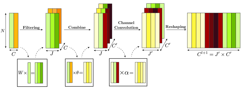
Figure 1: Manifold Filter-Combine Network architecture. Starting from a $C$-dimensional row vector-valued function, each layer in turn filters, combines, convolves channel-wise, applies a point-wise nonlinearity, and reshapes. For conciseness, we have omitted the point-wise activation in the figure.

Example 3.1 (Different Filters Along Each Channel).

If we set the cross-channel convolution equal to the identity, set $C_{\ell}^{\prime}=1$ and set $\theta_{i,k}^{(\ell,j)}=1$ then we obtain the layerwise update rule

If each of the $W_{j,k}^{(\ell)}=w^{(\ell)}_{j,k}(\mathcal{L}_{\rho})$ is a spectral filter (as defined in Section 2), we then obtain the layerwise update rule

$$f^{(\ell+1)}_{j}=\sigma\left(\sum_{k=1}^{C}w^{(\ell)}_{j,k}(\mathcal{L}_{\rho})f_{k}\right).$$

In the case where $\rho$ is constant and $\mathcal{L}_{\rho}$ is the Laplace-Beltrami operator, this coincides with the update rule which was introduced in [45] and has been subsequently studied in [44, 46, 48, 49, 13]. Notably, in this example the reshaping operator is the identity (since $C^{\prime}_{\ell}=1)$) and the filters $W_{j,k}^{(\ell)}$ depend on both the layer $\ell$ and the input channel $k$.

As mentioned above (see the discussion surrounding (15)), this class of networks is the most general and actually includes all MFCNs. However, considering, e.g., the filter and combine steps separately helps facilitate our analysis. For instance, our rate of convergence obtained in Theorem 3.7 depends on $\max_{j,k}(|\sum_{i=1}^{C_{\ell}}|\theta_{i,k}^{(\ell,j)}|),$ but unlike the results obtained in previous work does not directly depend on the width of the network. In particular, if we set $\theta_{i,k}^{(\ell,j)}=\frac{1}{C_{\ell}}$, then we have $\max_{j,k}(|\sum_{i=1}^{C_{\ell}}|\theta_{i,k}^{(\ell,j)}|)=1$.

Example 3.2 (Shared Filter Banks Along Each Channel).

In order to reduce the number of trainable parameters, it may be useful to utilize a (learned) filter bank which is shared across all input channels and a combination matrix which is shared across all filters. In this case, one obtains a layerwise update rule of the form (15). Such networks may loosely be thought of as a low-rank subset of the more general networks discussed in Example 3.1. (In this setting, since the filter banks are learned, there is still no need for cross-channel convolutions.)

Due to the irregularity of the data geometry, many popular GNNs such as the GCN of Kipf and Welling [25] use predesigned aggregations and incorporate learning through the combine steps. The next example discusses the analog of such networks on manifolds.

Example 3.3 (MCNs).

Set the cross-channel convolutions equal to the identity and let $J=J^{\prime}=1$. Let $\widetilde{A}$ be a fixed operator which should be thought of as either a low-pass filter or a localized averaging operator, and set $W^{(\ell)}_{i,1}=\widetilde{A}$ for all $i$. Let the matrix $\Theta^{(\ell)}=(\theta^{(\ell,1)}_{i,k})_{1\leq i\leq C_{\ell},1\leq k\leq C^{\prime}_{\ell}}$ be a learnable weight matrix. Then our layerwise update rule becomes $f_{k}^{\ell+1}=\sum_{i=1}^{C_{\ell}}\widetilde{A}f_{k}\theta_{i,k}^{(\ell,1)}$ which may be written compactly as $F^{(\ell+1)}=\sigma\left(\widetilde{A}F^{(\ell)}\Theta^{(\ell)}\right)$. Therefore, we obtain a network similar to the GCN of Kipf and Welling which we refer to as the manifold convolutional network (MCN). Notably, $\widetilde{A}$ can be designed in a variety of ways, but one possible choice is to define it in the spectral domain where $w$ is a non-increasing function such as an idealized low-pass filter $w(\lambda)=1_{\lambda\leq a}$ or setting $w(\lambda)=e^{-t\lambda}$ which corresponds to convolution against the heat kernel.

Additionally, one could consider the filter bank consisting of powers of $\widetilde{A},$ i.e. $W^{(\ell)}_{j}=\widetilde{A}^{j},$ $1\leq j\leq J$, use a different combine matrix in each channel, and employ a simple cross-channel convolution by setting $\alpha_{j,i}^{(\ell,k)}=1$. In this case, one obtains a layerwise update rule of the form $F^{(\ell+1)}=\sigma\left(\sum_{j=1}^{J}\widetilde{A}^{J}F^{(\ell)}\Theta^{(\ell,j)}\right)$, which can be thought of the manifold analog of the higher-order GCNs considered in work such as [27].

Similar to the above example, one could also consider the manifold analogs of other popular spectral GNNs such as ChebNet[17] or CayleyNet[28]. Our framework also includes several variations of the manifold scattering transform.

Example 3.4 (Hand-crafted Scattering Networks).

Let $\{W_{j}\}_{j=1}^{J}$ be a predesigned collection of filters, which are thought of as wavelets and do not depend on the layer or the input channel. Set the combine and cross-channel convolutions equal to the identity. One then obtains an entirely predesigned, multilayered network known as the manifold scattering transform. Such networks were considered in [36] in order to analyze the stability of and invariance properties of deep learning architectures defined on manifolds, building off of analogous work for Euclidean data [29, 16, 33, 8, 24, 51] and graphs [20, 19, 57, 21, 35, 4].

Example 3.5 (Learnable Scattering Networks).

For both Euclidean data and graphs, there have been a variety of papers that have introduced learning into the scattering framework.

In the Euclidean setting, [34] created a network that acts as a hybrid of the scattering transform and a CNN using predesigned, wavelet filter in some layers and learnable filters in others. Subsequent work by [55] introduced learning in a different way, incorporating cross-channel convolutions into an otherwise predesigned network. One may construct an analogous MFCN that corresponds to utilizing a predesigned filter bank $\{W_{j}\}_{j=1}^{J}$ which is shared across all channels, setting the combine step equal to the identity, and letting $\alpha_{j,i}^{(\ell,k)}$ be learnable. (Traditionally, scattering networks have used $|\cdot|$ as the activation function, but one could readily use other choices instead.)

In the graph setting, [50] incorporated learning into the scattering framework by utilizing predesigned wavelet filters, but learnable combine matrices (along with a few other features to boost performance). In a different approach, [40] sought to relax the graph scattering transform by replacing dyadic scales $2^{j}$ with an increasing sequence of scales $t_{j}$ which are learned from data via a selector matrix. To obtain an analogous MFCN, we set $W_{j}=e^{-j\mathcal{L}_{\rho}}$ for $0\leq j\leq J$, which diffuses the input signal over the manifold at different time-scales, corresponding to the diffusion module utilized in [40]. We then set the combination step equal to the identity and learn relationships between the diffusion scales via cross-channel convolutions (where the cross-channel convolutions utilized in [40] have a certain structure that encourages the network to behave in a wavelet-like manner). Additionally, as has previously been noted in [40], these two forms of learnable geometric scattering are compatible and one could readily utilize learnable combine steps while also using cross-channel convolutions to learn relationships between diffusion scales.

Lastly, we also note that our framework includes simple multilayer perceptrons.

Example 3.6 (Multilayer Perceptron).

If one sets $J_{\ell}=1$ and sets both $W_{1,k}^{(\ell)}$ and the cross-channel convolution to be the identity operator then one obtains a simple dense layer that does not utilize the geometry of the manifold. In some sense, this is contrary to our goal of developing networks that utilize the manifold structure of the data. However, including some simple dense layers might nevertheless be useful for, for example, reducing the number of channels in the network.

3.1 Implementation from point clouds

As alluded to earlier, in many applications one does not have global knowledge of the manifold $\mathcal{M}$ and merely has access to $n$ data points $\{x_{j}\}_{j=1}^{n}$ and evaluations of $F$ at those data points. This leads us to recall the normalized evaluation operator $(P_{n}f)(j)=\frac{1}{\sqrt{n}}f(x_{j})$ and approximate $F$ by an $n\times C$ data matrix $\mathbf{X}=(\mathbf{x}_{1},\ldots,\mathbf{x}_{C})$, where $\mathbf{x}_{k}=P_{n}f_{k}$. One may then implement an approximation of the network via the discrete update rules.

Filtering: $$\quad\tilde{\mathbf{x}}^{(\ell)}_{j,k}=\mathbf{W}^{(\ell)}_{j,k}\mathbf{x}^{(\ell)}_{k},\quad 1\leq j\leq J_{\ell},1\leq k\leq C_{\ell}$$

Combine: $$\quad\mathbf{y}_{j,k}^{(\ell)}=\sum_{i=1}^{C_{\ell}}\tilde{\mathbf{x}}^{(\ell)}_{j,i}\theta^{(\ell,j)}_{i,k},\quad 1\leq j\leq J_{\ell},1\leq k\leq C^{\prime}_{\ell}$$

Cross-Channel Convolution: $$\quad\tilde{\mathbf{y}}^{(\ell)}_{j,k}=\sum_{i=1}^{J_{\ell}}\alpha^{(\ell,k)}_{j,i}\mathbf{y}_{i,k},1\leq j\leq J_{\ell}^{\prime},1\leq k\leq C^{\prime}_{\ell}$$

Activation: $$\quad\mathbf{z}_{j,k}^{(\ell)}=\sigma\circ\tilde{\mathbf{y}}_{j,k}^{(\ell)},\quad 1\leq j\leq J_{\ell},1\leq k\leq C^{\prime}_{\ell}$$

Reshaping: $$\quad\mathbf{x}^{(\ell+1)}_{(j-1)C_{\ell}+k}=\mathbf{z}^{(\ell)}_{j,k},1\leq j\leq J_{\ell}^{\prime},1\leq k\leq C^{\prime}_{\ell}$$

where $\mathbf{W}_{j,k}^{(\ell)}$ is a matrix which acts as a discrete approximation of $W_{j,k}^{(\ell)}$.

The following theorem shows that the discrete implementation will converge to its continuum counterpart in the sense that $P_{n}F^{(\ell)}\approx\mathbf{X}^{(\ell)}$ if the matrices $\mathbf{W}_{j,k}^{(\ell)}$ are designed so that $\mathbf{W}_{j,k}^{(\ell)}P_{n}f_{k}^{(\ell)}\approx P_{n}W_{j,k}f_{k}^{(\ell)}$. For a proof, please see Appendix C.

Theorem 3.7.

Let $f\in\mathcal{C}(\mathcal{M})$, and suppose that for all $\ell$, there exists $\epsilon_{\ell,n}>0$ such that we have

$$\|P_{n}W_{j,k}^{(\ell)}f_{k}^{(\ell)}-\mathbf{W}^{(\ell)}_{j,k}\mathbf{x}^{(\ell)}_{k}\|_{2}\leq\|\mathbf{x}^{(\ell)}_{k}-P_{n}f_{k}^{\ell}\|_{2}+\epsilon_{\ell,n}$$

for all $1\leq k\leq C_{\ell}$. Let $A_{1}^{(\ell)}=\max_{j,k}(|\sum_{i=1}^{C_{\ell}}|\theta_{i,k}^{(\ell,j)}|),$ $A_{2}^{(\ell)}=\max_{j,k}(\sum_{i=1}^{J_{\ell}}|\alpha_{j,i}^{(\ell,k)}|)$ and assume that $\sigma$ is non-expansive, i.e. $|\sigma(x)-\sigma(y)|\leq|x-y|$. Then,

$$\|\mathbf{x}_{k}^{\ell}-P_{n}f_{k}^{\ell}\|_{2}\leq\sum_{i=0}^{\ell-1}\prod_{j=i}^{\ell-1}A_{1}^{(j)}A_{2}^{(j)}\epsilon_{i,n}.$$

Notably, Theorem 3.7 does not assume the filters are constructed in the spectral domain nor does it assume they have any particular form. It is a general result that shows that if individual filters converge, then so does the multilayer network. Moreover, if the weights $\alpha_{j,i}^{(\ell,k)}$ and $\theta_{j,i}^{(\ell,j)}$ are normalized so that the $A_{1}^{(j)}=A_{2}^{(j)}=1,$ then the rate of the convergence is linear in the depth of the network. This is in contrast to previous results in [13, 49] whose rate of convergence featured an explicit exponential dependence on the depth of the network. (A similar exponential dependence was also encountered in [38] where the limiting object is a graphon rather than a manifold.)

Combining Theorem 3.7 with Theorem 2.2 immediately leads to the following corollary which gives a quantitative rate of convergence for Manifold Filter-Combine Networks constructed utilizing spectral filters when either the filter or the input signals are bandlimited. Notably, if one proves theorems analogous to Theorem 2.2 for other classes of filters (constructed either by spectral or not spectral methods) such as the $\alpha$-FDT filters considered in [45] or the closely related $\gamma$-FDT filters considered in [46], then one may immediately obtain similar corollaries.

Corollary 3.8.

Assume that each $W_{j,k}^{(\ell)}$ is a spectral filter of the form $W_{j,k}^{(\ell)}=w_{j,k}^{(\ell)}(\mathcal{L}_{\rho})$ with $\|w_{j,k}^{(\ell)}\|_{\mathbf{L}^{\infty}([0,\infty))}\leq 1$, and the matrices $\mathbf{W}_{j,k}$ are given by $\mathbf{W}_{j,k}^{(\ell)}=w_{j,k}^{(\ell)}(\mathbf{L}_{n})$. As in Theorem 3.7, let $A_{1}^{(\ell)}=\max_{j,k}(|\sum_{i=1}^{C_{\ell}}|\theta_{i,k}^{(\ell,j)}|),$ $A_{2}^{(\ell)}=\max_{j,k}(\sum_{i=1}^{C_{\ell}}|\alpha_{j,i}^{(\ell,k)}|)$ and assume that $\sigma$ is non-expansive, i.e. $|\sigma(x)-\sigma(y)|\leq|x-y|$. Let $A^{(\ell)}_{\text{maxLip}}=\max_{j,k,}A_{\text{Lip}}(w^{(\ell)}_{j,k}).$ Assume that there exist sequences of real numbers $\{\alpha_{n}\}_{n=1}^{\infty}$, $\{\beta_{n}\}_{n=1}^{\infty}$, $\{\gamma_{n}\}_{n=1}^{\infty}$, with $\lim_{n\rightarrow\infty}\alpha_{n}=\lim_{n\rightarrow\infty}\beta_{n}=\lim_{n\rightarrow\infty}\gamma_{n}=0,$ such that for all $1\leq i\leq\kappa$ and for $n$ sufficiently large, we have

(16) $$|\lambda_{i}-\lambda^{n}_{i}|\leq\alpha_{n},\quad\|P_{n}\phi_{i}-\phi_{i}^{n}\|_{2}\leq\beta_{n},\quad|\langle P_{n}f,P_{n}g\rangle_{2}-\langle f,g\rangle_{\mathbf{L}^{2}(\mathcal{M})}|\leq\gamma_{n}^{2}\|f\|_{\mathbf{L}^{4}(\mathcal{M})}\|g\|_{\mathbf{L}^{4}(\mathcal{M})}.$$

Assume $n$ is large enough such that (16) holds and $\alpha_{n}A^{(i)}_{\text{maxLip}},\beta_{n},\gamma_{n}\|\phi_{j}\|_{\mathbf{L}^{4}(\mathcal{M})}\leq 1$ for all $i\leq\ell$ and $j\leq\kappa$. Then, the error in each channel of the $\ell$-th layer satisfies

$$\|\mathbf{x}_{k}^{\ell}-P_{n}f_{k}^{\ell}\|_{2}\leq\sum_{i=0}^{\ell-1}\prod_{j=i}^{\ell-1}A_{1}^{(j)}A_{2}^{(j)}6\kappa\max_{k^{\prime}}\left((A^{(i)}_{\text{maxLip}}\alpha_{n}+\beta_{n})\|f^{(i)}_{k^{\prime}}\|_{\mathbf{L}^{2}(\mathcal{M})}+\gamma_{n}\|f^{(i)}_{k^{\prime}}\|_{\mathbf{L}^{4}(\mathcal{M})}\right).$$

In particular, if we assume that we have $A_{1}^{(j)},A_{2}^{(j)},A^{(i)}_{\text{maxLip}}\leq 1$, for all $i$ and $j$ we have

$$\|\mathbf{x}_{k}^{\ell}-P_{n}f_{k}^{\ell}\|_{2}\leq C_{\mathcal{M}}\kappa\ell\left((\alpha_{n}+\beta_{n})\max_{k^{\prime},i}\|f^{(i)}_{k^{\prime}}\|_{\mathbf{L}^{2}(\mathcal{M})}+\gamma_{n}\max_{k^{\prime},i}\|f^{(i)}_{k^{\prime}}\|_{\mathbf{L}^{4}(\mathcal{M})}\right).$$

In Section 2.1, we provided several examples of $\alpha_{n},\beta_{n}$, and $\gamma_{n}$ for three graph constructions. Using Corollary 3.8 and Lemma 2.4, we immediately obtain the following three corollaries giving rates of convergence for each of these constructions.

Corollary 3.9.

Assume the same conditions on $W_{j,k}^{(\ell)}$, $\mathbf{W}_{j,k}$, $A_{1}^{(\ell)}$, $A_{2}^{(\ell)}$, $A^{(\ell)}_{\text{maxLip}}$, and $\sigma$ as in Corollary 3.8, and assume $A_{1}^{(j)},A_{2}^{(j)},A^{(i)}_{\text{maxLip}}\leq 1$. As in Example 2.5, assume that $\rho$ is constant so that $\mathcal{L}_{\rho}$ is the Laplace-Beltrami operator and assume $\mathbf{G}_{n}$ is constructed with a Gaussian kernel (using the same parameter choices as in Example 2.5). Then with probability $1-\mathcal{O}(\frac{1}{n^{9}})$, for large enough $n$, the error in each channel of the $\ell$-th layer of the MFCN satisfies

$$\|\mathbf{x}_{k}^{\ell}-P_{n}f_{k}^{\ell}\|_{2}\leq C_{\mathcal{M}}\kappa\ell\left(\frac{\sqrt{\log(n)}}{n^{2/(d+6)}}\max_{k^{\prime},i}\|f^{(i)}_{k^{\prime}}\|_{\mathbf{L}^{2}(\mathcal{M})}+\left(\frac{\log n}{n}\right)^{1/4}\max_{k^{\prime},i}\|f^{(i)}_{k^{\prime}}\|_{\mathbf{L}^{4}(\mathcal{M})}\right).$$

Corollary 3.10.

Assume the same conditions on $W_{j,k}^{(\ell)}$, $\mathbf{W}_{j,k}$, $A_{1}^{(\ell)}$, $A_{2}^{(\ell)}$, $A^{(\ell)}_{\text{maxLip}}$, and $\sigma$ as in Corollary 3.8, and assume $A_{1}^{(j)},A_{2}^{(j)},A^{(i)}_{\text{maxLip}}\leq 1$. As in Example 2.6, assume that $\mathcal{L}_{\rho}f=-\frac{1}{2\rho}\text{div}(\rho^{1-2/d}\nabla f)$ and that $\mathbf{G}_{n}$ is an $\epsilon$-graph (with $\epsilon$ chosen as in Example 2.6). Then with probability $1-\mathcal{O}(\frac{1}{n^{9}})$, for large enough $n$, the error in each channel of the $\ell$-th layer of the MFCN satisfies

$$\|\mathbf{x}_{k}^{\ell}-P_{n}f_{k}^{\ell}\|_{2}\leq C_{\mathcal{M}}\kappa\ell\left(\left(\frac{\log(n)}{n}\right)^{\frac{1}{d+4}}\max_{k^{\prime},i}\|f^{(i)}_{k^{\prime}}\|_{\mathbf{L}^{2}(\mathcal{M})}+\left(\frac{\log n}{n}\right)^{1/4}\max_{k^{\prime},i}\|f^{(i)}_{k^{\prime}}\|_{\mathbf{L}^{4}(\mathcal{M})}\right).$$

Corollary 3.11.

Assume the same conditions on $W_{j,k}^{(\ell)}$, $\mathbf{W}_{j,k}$, $A_{1}^{(\ell)}$, $A_{2}^{(\ell)}$, $A^{(\ell)}_{\text{maxLip}}$, and $\sigma$ as in Corollary 3.8, and assume $A_{1}^{(j)},A_{2}^{(j)},A^{(i)}_{\text{maxLip}}\leq 1$. As in Example 2.7, let $\mathcal{L}_{\rho}f=-\frac{1}{2\rho}\text{div}(\rho^{1-2/d}\nabla f)$ and assume that $\mathbf{G}_{n}$ is constructed as a $k$-NN (with $k$ chosen as in Example Example 2.7). Then with probability $1-\mathcal{O}(\frac{1}{n^{9}})$, for large enough $n$, the error in each channel of the $\ell$-th layer of the MFCN satisfies

$$\|\mathbf{x}_{k}^{\ell}-P_{n}f_{k}^{\ell}\|_{2}\leq C_{\mathcal{M}}\kappa\ell\left(\left(\frac{\log(n)}{n}\right)^{\frac{1}{d+4}}\max_{k^{\prime},i}\|f^{(i)}_{k^{\prime}}\|_{\mathbf{L}^{2}(\mathcal{M})}+\left(\frac{\log n}{n}\right)^{1/4}\max_{k^{\prime},i}\|f^{(i)}_{k^{\prime}}\|_{\mathbf{L}^{4}(\mathcal{M})}\right).$$

4 Numerical Experiments

In this section, we compare the performance of several different manifold filter-combine networks on the ModelNet dataset[53] which was previously considered in, e.g., [48] and on a single-cell data set which was previously considered in [12]. In particular, we focus on the MNN with different learnable filters in each channel (DLF), the MCN, a hand-crafted scattering network (Scattering), and a learnable scattering network (Learnable Scattering) discussed in Examples 3.1, 3.3, 3.4 and 3.5. The code for reproducing our experiments is available at https://github.com/KrishnaswamyLab/mfcn.

4.1 Data

We evaluate the different models on two datasets: the widely used ModelNet10 dataset and a single-cell dataset from melanoma patients.

ModelNet10

The ModelNet10 dataset consists of three-dimensional point clouds sampled from various objects belonging to the classes bathtub, bed, chair, desk, dresser, monitor, nightstand, sofa, table, and toilet. Examples of point clouds in the dataset are given in Fig. 2. For each point cloud, we preprocess the data by scaling the point coordinates (z-scaling), and then randomly sampling 100 points from the whole point cloud. We then create a graph via the constructions discussed in Examples 2.5, 2.6, and 2.7, i.e., Gaussian kernels (dense), $\epsilon$-graphs, and unweighted k-NN graphs. We use the $x$, $y$, and $z$ coordinates of the nodes as input signals. The ModelNet10 dataset comes with a predefined training set (3901 samples) and test set (799 samples). In our experiments, we randomly select 20% of the training set to use for validation. We then consider two regimes. In the full data regime, we use the entire remaining 80% of for training. In the subset data regime, we randomly select 1000 samples from that 80% to use for training. We repeat this procedure five times and report our accuracies in the format mean $\pm$ std.

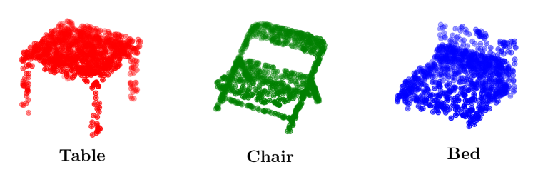
Figure 2: Examples of point clouds from the ModelNet10 dataset. 1000 points are shown per shape. In our experiments, we only used 100 samples per shape.

Melanoma

This dataset, which was originally collected in [37], includes single-cell protein measurements on immune cells obtained from melanoma patients and featurized using the log-transformed $\ell^{1}$-normalized protein expression feature data of the cell. 11,862 T lymphocytes from core tissue sections were taken from 54 patients diagnosed with various stages of melanoma and 30 proteins were measured per cell. All of the patients received checkpoint blockade immunotherapy, which licenses the patient’s T cells to kill tumor cells. Our goal is to characterize the immune status of patients prior to treatment and to predict which patients will respond well versus which patients will not.

In our context, each cell corresponds to a point in high-dimensional space, and a patient’s immunological state is characterized by the point cloud of the available cells. We may then view separating responders from non-responders as a binary manifold classification task. (For further details, please see [12] and the references within.) To increase the size of the data set, for each patient, we subsampled 400 cells from the original point cloud and repeated this procedure ten times, resulting in a total of 540 point clouds. However, in our training/testing/validation splits, we made sure to keep all point clouds from the same patient in the same split.

4.2 Models

In our experiments, we consider several manifold neural network architectures described below. For each model, we used two layers of manifold networks, followed by a multi-layer perceptron classifier consisting of a single hidden layer. For further details of our hyperparameter settings and training procedures please see Table 3 in Section D.

Scattering and Learnable Scattering

We follow the experimental procedure utilized in [14] and compute zeroth-, first-, and second-order scattering moments. More specifically, for $0\leq j\leq J$ and $1\leq q\leq Q$, we define first-order, $q$-th scattering moments by

$$Sf[j,q]\coloneqq\int_{\mathcal{M}}|W_{j}f(x)|^{q}dx=\|W_{j}f\|_{\mathbf{L}^{q}(\mathcal{M})}^{q},$$

where $W_{j}$ are spectral wavelet filters corresponding to the functions $w_{j}(\lambda)=e^{-2^{j-1}\lambda}-e^{-2^{j}\lambda}$ for $1\leq j\leq J$ and $w_{0}(\lambda)=1-e^{-\lambda}$. We define second-order moments, for $0\leq j<j^{\prime}\leq J$, by

$$Sf[j,j^{\prime},q]\coloneqq\int_{\mathcal{M}}|W_{j^{\prime}}|W_{j}f(x)||^{q}dx=\|W_{j^{\prime}}|W_{j}f|\|_{\mathbf{L}^{q}(\mathcal{M})}^{q}.$$

Zeroth-order moments are defined simply by

$$Sf[q]\coloneqq\int_{\mathcal{M}}|f(x)|^{q}dx=\|f\|_{\mathbf{L}^{q}(\mathcal{M})}^{q}.$$

In our experiments, we set $J=4$, $Q=4$. We considered one version of the scattering transform (Scattering Spectral) in which the wavelets were constructed using the first 20 eigenvalues and another (Scattering Approx) in which the heat-kernel is approximated via a lazy random walk matrix $\mathbf{P}=\frac{1}{2}(\mathbf{I}+\mathbf{A}\mathbf{D}^{-1})$. Additionally, we also considered a learnable version of the graph scattering transform (Learnable Scattering) in which we implemented the manifold analog of the learnable geometric scattering network introduced in [40]. (In this network, dyadic scales are replaced by a sequence of scales learned from data. Please see [40] for details.)

DLF

We used two layers of DLF, where each layer consists of $J_{\ell}$ spectral filters ($J_{1}=16,J_{2}=32)$. After applying the $J_{\ell}$ filters per input dimensions, we combined the channels by summation (i.e., $\theta^{(\ell,j)}_{i,k}=1$). Similarly to scattering, we used the first 20 eigenvalues and eigenvectors of the Laplacian matrix to compute our filters. We used a ReLU activation and the identity map for the cross-channel convolution. We used average pooling at the last layer to obtain the feature vector to be processed by the classifier. We considered two parameterizations of the filters $w(\lambda)$, one denoted DLF-MLP, where we parametrize each $w(\lambda)$ as a 2-layer MLP, and the other denoted DLF-POLY, in which we parameterize each $w(\lambda)$ as a degree-four polynomial of $e^{-\lambda}$ (which is the parameterization utilized in, e.g., [48]).

MCN

We used two layers of graph convolutional networks with $J_{l}$ ($J_{1}=16,J_{2}=32)$ hidden dimension applied to the input graph with ReLU activations. As in [25], our low-pass filter was implemented by $\hat{\mathbf{A}}=(\mathbf{D}+\mathbf{I})^{-1/2}(\mathbf{A}+\mathbf{I})(\mathbf{D}+\mathbf{I})^{-1/2}$ which is equivalent to applying the spectral filter $w(\lambda)=1-\lambda/2$ to the normalized graph Laplacian and then utilizing a renormalization trick in order to facilitate the learning process. We used a ReLU activation and the identity map for the cross-channel convolution. We used average pooling at the last layer to obtain the feature vector to be processed by the classifier.

4.3 Results

We compared the performance of the different models and graph construction based on the classification accuracy on the left-out test set. In Table 1, we report the mean and standard deviation of the test accuracy on ModelNet10 across the five different splits (5-folds) for both the full and subset data regimes.

Full Data Regime Subset Data Regime Graph type Dense Epsilon k-NN Dense Epsilon k-NN # params Time MCN 0.54 $\pm$ 0.02 0.63 $\pm$ 0.01 0.71 $\pm$ 0.02 0.44 $\pm$ 0.03 0.57 $\pm$ 0.02 0.64 $\pm$ 0.02 0.9K 181 s. DLF-MLP 0.75 $\pm$ 0.02 0.75 $\pm$ 0.02 0.73 $\pm$ 0.01 0.66 $\pm$ 0.01 0.7 $\pm$ 0.02 0.66 $\pm$ 0.03 19K 291 s. DLF-POLY 0.69 $\pm$ 0.01 0.69 $\pm$ 0.02 0.74 $\pm$ 0.01 0.63 $\pm$ 0.01 0.62 $\pm$ 0.02 0.69 $\pm$ 0.02 3.2K 303 s. Scattering Spectral 0.77 $\pm$ 0.01 0.74 $\pm$ 0.01 0.72 $\pm$ 0.03 0.72 $\pm$ 0.02 0.67 $\pm$ 0.02 0.62 $\pm$ 0.03 9.4K 368 s. Scattering Approx 0.81 $\pm$ 0.01 0.79 $\pm$ 0.0 0.7 $\pm$ 0.02 0.76 $\pm$ 0.02 0.75 $\pm$ 0.01 0.61 $\pm$ 0.01 9.4K 352 s. Learnable Scattering 0.82 $\pm$ 0.01 0.81 $\pm$ 0.01 0.78 $\pm$ 0.01 0.79 $\pm$ 0.01 0.76 $\pm$ 0.02 0.73 $\pm$ 0.02 9.5K 679 s.

Table 1: Test accuracies on ModelNet10 for the MCN, DLF, and Scattering methods. We report means and standard deviations. Models were evaluated for the dense, epsilon, and k-NN graph constructions. We trained the models on the full dataset (3192 training samples - full data regime) and on a subset of it (1000 training samples - subset data regime). Time refers to the training time of 20 epochs on the Epsilon graph in the subset data regime.

All of the models consistently perform much better than random chance (which is roughly $10\%$ accuracy since there are ten classes) but are all far from 100% accuracy. In particular, in the full data regime, accuracy levels range from 54% to 82% and from 44% to 79% in the subset data regime. Overall, Learnable Scattering is the best performing method, particularly on the Dense graphs and the Epsilon Graphs. We note that DLF-MLP outperforms DLF-POLY in four out of six cases, but has the drawback of requiring more parameters. On the $k$-NN graphs, MCN performs nearly as well as DLF, but is the least accurate method on the dense graph construction.

In Table 2, we report the mean and standard deviation of the test accuracy on the melanoma dataset across the five different splits (5-folds). Here we observe a more mixed picture. Learnable Scattering is the top performing method for the dense graph construction, where DLF-Poly and DLF-MLP are the top methods for Epsilon and k-NN graphs respectively. We note that the low effective number of samples also results in higher variance across folds. Additionally, we note that the results for the hand-crafted scattering network reported here are significantly lower than the 83% accuracy obtained in [12]. This discrepancy is likely due to the fact that [12] used a decision-tree to perform the final classification rather than dense layers. (Our setup also differs from that used in [12]in the sense that [12] did not perform any subsampling of the point clouds.)

Graph type Dense Epsilon KNN MCN 0.74 $\pm$ 0.1 0.64 $\pm$ 0.15 0.66 $\pm$ 0.16 DLF-MLP 0.64 $\pm$ 0.18 0.72 $\pm$ 0.08 0.75 $\pm$ 0.05 DLF-POLY 0.69 $\pm$ 0.17 0.77 $\pm$ 0.11 0.68 $\pm$ 0.08 Scattering (Spectral) 0.67 $\pm$ 0.06 0.65 $\pm$ 0.09 0.63 $\pm$ 0.05 Scattering (Approx) 0.69 $\pm$ 0.06 0.68 $\pm$ 0.02 0.64 $\pm$ 0.15 Learnable Scattering 0.75 $\pm$ 0.1 0.67 $\pm$ 0.14 0.7 $\pm$ 0.12

Table 2: Test accuracies on the Melanoma dataset for the MCN, DLF, and Scattering methods. We report means and standard deviations. Models were evaluated for the dense, epsilon, and k-NN graph constructions. We trained the models on a subsampled version of the dataset where each point clouds contains 400 points.

5 Conclusion

We have introduced a new framework for analyzing and implementing manifold neural networks that we call manifold filter-combine networks. This framework naturally allows us to think about many interesting classes of MNNs such as the manifold analogs of GCNs and several relaxed variations of the manifold scattering transform. Additionally, we have provided methods for implementing such networks when one does not have global knowledge of the manifold, but merely has access to $n$ sample points, that converge provably to their continuum limit as $n\rightarrow\infty$. In order to establish this result, we also prove a theorem establishing sufficient convergence conditions for the individual filters used in the network. Unlike related results in previous work, this result does not assume points are drawn from the uniform distribution and is not specific to any particular graph construction. Instead, it shows that if the eigenvectors and eigenvalues of the graph Laplacian converge (and additionally that discrete inner products converge to continuum inner products) then spectral filters constructed from the graph Laplacian will converge as well. This allows our results to be applied to a wide variety of graph constructions including those discussed in Examples 2.5, 2.6, and 2.7.

The flexibility of our setup is deliberate. The development of manifold neural networks is in its infancy, even compared to graph neural networks, and there are many questions about which networks will perform best in practice. Should networks use learnable filter banks similar to a CNN or predesigned averaging operations similar to a common aggregate-combine network? Are cross-channel convolutions a viable way to introduce learning in settings where there are no nontrivial relations between input channels?

In this work, we do not claim to provide an answer to the question “what are the best ways to design a manifold neural network?” which ultimately will need to be answered through thorough experimentation. The purpose of this paper is instead to facilitate this experimentation by providing a useful framework for thinking about MNNs. We also note several other important areas of future work. (i) In Examples 2.5, 2.6, and 2.7, we consider settings where the data points $\{x_{i}\}$ lie exactly on the manifold. Relaxing these assumptions would greatly increase the applicability of our theory to noisy real-world data. (ii) Most of the data sets used in the MNN literature focus on two-dimensional surfaces. Developing challenging and relevant benchmarks for learning on higher-dimensional manifolds would help facilitate the experimental exploration of various MNN architectures.

Appendix A The Proof of Lemma 2.4

Define random variables $\{X_{i}\}_{i=1}^{n}$ by $X_{i}\coloneqq f(x_{i})g(x_{i})$ and note that by definition we have

$$\langle P_{n}f,P_{n}g\rangle_{2}=\frac{1}{n}\sum_{i=1}^{n}f(x_{i})g(x_{i})=\frac{1}{n}\sum_{i=1}^{n}X_{i}.$$

Since the $x_{i}$ are sampled i.i.d. with density $\rho$, we have

$$\mathbb{E}[X_{i}]=\int_{\mathcal{M}}f(x)g(x)\rho(x)dx=\langle f,g\rangle_{\mathbf{L}^{2}(\mathcal{M})}.$$

Therefore, letting $\sigma^{2}\coloneqq\mathbb{E}[X_{i}^{2}]-\mathbb{E}[X_{i}]^{2}$ and $M\coloneqq\|fg-\mathbb{E}[X_{i}]\|_{\mathbf{L}^{\infty}(\mathcal{M})}$, we see that by Bernstein’s inequality, we have

$$\mathbb{P}(|\langle P_{n}f,P_{n}g\rangle_{2}-\langle f,g\rangle_{\mathbf{L}^{2}(\mathcal{M})}|>\eta) =\mathbb{P}\left(\left|\frac{1}{n}\sum_{i=1}^{n}X_{i}-\frac{1}{n}\sum_{i=1}^{n}\mathbb{E}[X_{i}]\right|>\eta\right)$$

$$=\mathbb{P}\left(\left|\sum_{i=1}^{n}X_{i}-\sum_{i=1}^{n}\mathbb{E}[X_{i}]\right|>n\eta\right)$$

$$\leq 2\exp\left(-\frac{\frac{1}{2}n\eta^{2}}{\sigma^{2}+\frac{1}{3}M\eta}\right).$$

Setting $\eta=6\sqrt{\dfrac{\sigma^{2}\log(n)}{n}}$, we see that for $n$ large enough so that $1+\dfrac{M\eta}{3\sigma^{2}}<2$, we have

$$\mathbb{P}(|\langle P_{n}f,P_{n}g\rangle_{2}-\langle f,g\rangle_{\mathbf{L}^{2}(\mathcal{M})}|>\eta) \leq 2\exp\left(-\frac{18\sigma^{2}\log(n)}{\sigma^{2}+\frac{1}{3}M\eta}\right)$$

$$=2\exp\left(-\frac{18\log(n)}{1+\frac{M\eta}{3\sigma^{2}}}\right)$$

$$<2\exp\left(-9\log(n)\right)$$

$$=\frac{2}{n^{9}}.$$

We note that $\sigma^{2}\leq\mathbb{E}[X_{i}^{2}]=\langle f^{2},g^{2}\rangle_{\mathbf{L}^{2}(\mathcal{M})}$. Therefore, by the Cauchy-Schwarz inequality, with probability at least $1-\frac{2}{n^{9}}$, we have

$$|\langle P_{n}f,P_{n}g\rangle_{2}-\langle f,g\rangle_{\mathbf{L}^{2}(\mathcal{M})}| \leq 6\sqrt{\frac{\sigma^{2}\log(n)}{n}}$$

$$\leq 6\sqrt{\frac{\log(n)}{n}}\sqrt{\langle f^{2},g^{2}\rangle_{\mathbf{L}^{2}(\mathcal{M})}}$$

$$\leq 6\sqrt{\frac{\log(n)}{n}}\|f\|_{\mathbf{L}^{4}(\mathcal{M})}\|g\|_{\mathbf{L}^{4}(\mathcal{M})}.$$

Appendix B The Proof of Theorem 2.2

Proof B.1.

We first note that if either $w$ or $f$ is $\kappa$-bandlimited, we have

$$\|w(\mathbf{L}_{n})P_{n}f-P_{n}w(\mathcal{L}_{\rho})f\|_{2}$$

$$= \left\|\sum_{i=1}^{\kappa}w(\lambda_{i}^{n})\langle P_{n}f,\phi_{i}^{n}\rangle_{2}\phi_{i}^{n}-\sum_{i=1}^{\kappa}w(\lambda_{i})\langle f,\phi_{i}\rangle_{\mathcal{M}}P_{n}\phi_{i}\right\|_{2}$$

(17) $$\leq \left\|\sum_{i=1}^{\kappa}(w(\lambda_{i}^{n})-w(\lambda_{i}))\langle P_{n}f,\phi_{i}^{n}\rangle_{2}\phi_{i}^{n}\right\|_{2}+\left\|\sum_{i=1}^{\kappa}w(\lambda_{i})(\langle P_{n}f,\phi_{i}^{n}\rangle_{2}\phi_{i}^{n}-\langle f,\phi_{i}\rangle_{\mathcal{M}}P_{n}\phi_{i})\right\|_{2}.$$

To bound the first term from (17), we note that by the triangle inequality, the Cauchy-Schwarz inequality, and the assumption that $n$ is large enough so that $A_{\text{Lip}}(w)\alpha_{n}\leq 1$, we have

$$\left\|\sum_{i=1}^{\kappa}(w(\lambda_{i}^{n})-w(\lambda_{i}))\langle P_{n}f,\phi_{i}^{n}\rangle_{2}\phi_{i}^{n}\right\|_{2}\leq \max_{1\leq i\leq\kappa}|w(\lambda_{i}^{n})-w(\lambda_{i})|\sum_{i=1}^{\kappa}\|P_{n}f\|_{2}\|\phi_{i}^{n}\|^{2}_{2}$$

$$\leq A_{\text{Lip}}(w)\alpha_{n}\sum_{i=1}^{\kappa}\|P_{n}f\|_{2}\|\phi_{i}^{n}\|^{2}_{2}$$

$$\leq A_{\text{Lip}}(w)\kappa\alpha_{n}\|P_{n}f\|_{2}$$

$$\leq \kappa\left(A_{\text{Lip}}(w)\alpha_{n}\|f\|_{\mathbf{L}^{2}(\mathcal{M})}+\gamma_{n}\|f\|_{\mathbf{L}^{4}(\mathcal{M})}\right),$$

where we use the fact that $\|\phi_{i}^{n}\|_{2}^{2}=1$ and that

(18) $$\|P_{n}f\|_{2}\leq\left(\|f\|_{\mathbf{L}^{2}(\mathcal{M})}^{2}+\gamma_{n}^{2}\|f\|_{\mathbf{L}^{4}(\mathcal{M})}^{2}\right)^{1/2}\leq\|f\|_{\mathbf{L}^{2}(\mathcal{M})}+\gamma_{n}\|f\|_{\mathbf{L}^{4}(\mathcal{M})}.$$

Now, turning our attention to the second term from (17), we have

$$\left\|\sum_{i=1}^{\kappa}w(\lambda_{i})(\langle P_{n}f,\phi_{i}^{n}\rangle_{2}\phi_{i}^{n}-\langle f,\phi_{i}\rangle_{\mathbf{L}^{2}(\mathcal{M})}P_{n}\phi_{i})\right\|_{2}$$

(19) $$\leq \left\|\sum_{i=1}^{\kappa}w(\lambda_{i})\langle P_{n}f,\phi_{i}^{n}\rangle_{2}(\phi_{i}^{n}-P_{n}\phi_{i})\right\|_{2}+\left\|\sum_{i=1}^{\kappa}w(\lambda_{i})(\langle P_{n}f,\phi_{i}^{n}\rangle_{2}-\langle f,\phi_{i}\rangle_{\mathbf{L}^{2}(\mathcal{M})}P_{n}\phi_{i}\right\|_{2}.$$

By the assumption (9), we have $\|\phi_{i}^{n}-P_{n}\phi_{i}\|_{2}\leq\beta_{n}$. Therefore, since $w$ is non-amplifying, we see

$$\left\|\sum_{i=1}^{\kappa}w(\lambda_{i})\langle P_{n}f,\phi_{i}^{n}\rangle_{2}(\phi_{i}^{n}-P_{n}\phi_{i})\right\|_{2} \leq\kappa\max_{1\leq i\leq\kappa}|\langle P_{n}f,\phi_{i}^{n}\rangle_{2}|\|\phi_{i}^{n}-P_{n}\phi_{i}\|_{2}$$

$$\leq\kappa\beta_{n}\|P_{n}f\|_{2}$$

(20) $$\leq\kappa\left(\beta_{n}\|f\|_{\mathbf{L}^{2}(\mathcal{M})}+\gamma_{n}\|f\|_{\mathbf{L}^{4}(\mathcal{M})}\right),$$

where the final inequality follows from (18) and the assumption that $n$ is large enough so that $\beta_{n}\leq 1$. Meanwhile, the second term from (19) can be bounded by

$$\left\|\sum_{i=1}^{\kappa}w(\lambda_{i})(\langle P_{n}f,\phi_{i}^{n}\rangle_{2}-\langle f,\phi_{i}\rangle_{\mathcal{M}})P_{n}\phi_{i}\right\|_{2}$$

$$\leq \sum_{i=1}^{\kappa}|w(\lambda_{i})||\langle P_{n}f,\phi_{i}^{n}\rangle_{2}-\langle f,\phi_{i}\rangle_{\mathcal{M}}|\|P_{n}\phi_{i}\|_{2}$$

$$\leq \sum_{i=1}^{\kappa}|\langle P_{n}f,\phi_{i}^{n}\rangle_{2}-\langle f,\phi_{i}\rangle_{\mathcal{M}}|\|P_{n}\phi_{i}\|_{2}$$

$$\leq \sum_{i=1}^{\kappa}|\langle P_{n}f,\phi_{i}^{n}\rangle_{2}-\langle P_{n}f,P_{n}\phi_{i}\rangle_{2}|\|P_{n}\phi_{i}\|_{2}+\sum_{i=1}^{\kappa}|\langle P_{n}f,P_{n}\phi_{i}\rangle_{2}-\langle f,\phi_{i}\rangle_{\mathcal{M}}|\|P_{n}\phi_{i}\|_{2}.$$

By the Cauchy-Schwarz inequality, (9), (18), and the assumption that $n$ is large enough so that $\beta_{n}\leq 1$, we have

$$|\langle P_{n}f,\phi_{i}^{n}\rangle_{2}-\langle P_{n}f,P_{n}\phi_{i}\rangle_{2}| \leq\|P_{n}f\|_{2}\|\phi_{i}^{n}-P_{n}\phi_{i}\|_{2}$$

$$\leq\beta_{n}\left(\|f\|_{\mathbf{L}^{2}(\mathcal{M})}+\gamma_{n}\|f\|_{\mathbf{L}^{4}(\mathcal{M})}\right)$$

$$\leq\left(\beta_{n}\|f\|_{\mathbf{L}^{2}(\mathcal{M})}+\gamma_{n}\|f\|_{\mathbf{L}^{4}(\mathcal{M})}\right).$$

And also by (9) and (18) we have

$$|\langle P_{n}f,P_{n}\phi_{i}\rangle_{2}-\langle f,\phi_{i}\rangle_{2}|\leq\gamma_{n}^{2}\|f\|_{\mathbf{L}^{4}(\mathcal{M})}\|\phi_{i}\|_{\mathbf{L}^{4}(\mathcal{M})},\quad\text{and}\quad\|P_{n}\phi_{i}\|_{2}\leq 1+\gamma_{n}\|\phi_{i}\|_{\mathbf{L}^{4}(\mathcal{M})}.$$

Since $\kappa$ is fixed and $\lim_{n\rightarrow\infty}\gamma_{n}=0,$ for sufficiently large $n$ we have $\gamma_{n}\|\phi_{i}\|_{\mathbf{L}^{4}(\mathcal{M})}\leq 1$ for all $i\leq\kappa.$ This implies

$$|\langle P_{n}f,P_{n}\phi_{i}\rangle_{2}-\langle f,\phi_{i}\rangle_{2}|\leq\gamma_{n}\|f\|_{\mathbf{L}^{4}(\mathcal{M})},\quad\text{and}\quad\|P_{n}\phi_{i}\|_{2}\leq 1+\gamma_{n}\|\phi_{i}\|_{\mathbf{L}^{4}(\mathcal{M})}\leq 2.$$

Therefore, the second term from (19) can be bounded by

$$\left\|\sum_{i=1}^{\kappa}w(\lambda_{i})(\langle P_{n}f,\phi_{i}^{n}\rangle_{2}-\langle f,\phi_{i}\rangle_{\mathcal{M}})P_{n}\phi_{i}\right\|_{2}$$

$$\leq \sum_{i=1}^{\kappa}|\langle P_{n}f,\phi_{i}^{n}\rangle_{2}-\langle P_{n}f,P_{n}\phi_{i}\rangle_{2}|\|P_{n}\phi_{i}\|_{2}+\sum_{i=1}^{\kappa}|\langle P_{n}f,P_{n}\phi_{i}\rangle_{2}-\langle f,\phi_{i}\rangle_{2}|\|P_{n}\phi_{i}\|_{2}$$

$$\leq \sum_{i=1}^{\kappa}\left(\beta_{n}\|f\|_{\mathbf{L}^{2}(\mathcal{M})}+\gamma_{n}\|f\|_{\mathbf{L}^{4}(\mathcal{M})}\right)\|P_{n}\phi_{i}\|_{2}+\sum_{i=1}^{\kappa}\gamma_{n}\|f\|_{\mathbf{L}^{4}(\mathcal{M})}\|P_{n}\phi_{i}\|_{2}$$

(21) $$\leq 4\kappa\left(\beta_{n}\|f\|_{\mathbf{L}^{2}(\mathcal{M})}+\gamma_{n}\|f\|_{\mathbf{L}^{4}(\mathcal{M})}\right).$$

Therefore, combining Equations (17) through (21) yields

$$\|w(\mathbf{L}_{n})P_{n}f-P_{n}w(\mathcal{L}_{\rho})f\|_{2}$$

$$\leq \left\|\sum_{i=1}^{\kappa}(w(\lambda_{i}^{n})-w(\lambda_{i}))\langle P_{n}f,\phi_{i}^{n}\rangle_{2}\phi_{i}^{n}\right\|_{2}+\left\|\sum_{i=1}^{\kappa}w(\lambda_{i})(\langle P_{n}f,\phi_{i}^{n}\rangle_{2}\phi_{i}^{n}-\langle f,\phi_{i}\rangle_{\mathcal{M}}P_{n}\phi_{i})\right\|_{2}$$

$$\leq \kappa(A_{\text{Lip}}(w)\alpha_{n}\|f\|_{\mathbf{L}^{2}(\mathcal{M})}+\gamma_{n}\|f\|_{\mathbf{L}^{4}(\mathcal{M})})+5\kappa\left(\beta_{n}\|f\|_{\mathbf{L}^{2}(\mathcal{M})}+\gamma_{n}\|f\|_{\mathbf{L}^{4}(\mathcal{M})}\right)$$

$$\leq 6\kappa\left((A_{\text{Lip}(w)}\alpha_{n}+\beta_{n})\|f\|_{\mathbf{L}^{2}(\mathcal{M})}+\gamma_{n}\|f\|_{\mathbf{L}^{4}(\mathcal{M})}\right)$$

thus completing the proof of (10).

To prove (11), we observe that since $\|w\|_{\mathbf{L}^{\infty}([0,\infty))}\leq 1,$ we have

(22) $$\|w(\mathbf{L}_{n})\mathbf{x}-w(\mathbf{L}_{n})P_{n}f\|_{2}\leq\|\mathbf{x}-P_{n}f\|_{2}$$

by the same reasoning as (8). Therefore, by the triangle inequality, we have

$$\|w(\mathbf{L}_{n})\mathbf{x}-P_{n}w(\mathcal{L}_{\rho})f\|_{2}\leq \|w(\mathbf{L}_{n})\mathbf{x}-w(\mathbf{L}_{n})P_{n}f\|_{2}+\|w(\mathbf{L}_{n})P_{n}f-P_{n}w(\mathcal{L}_{\rho})f\|_{2}$$

$$\leq \|\mathbf{x}-P_{n}f\|_{2}+6\kappa\left((A_{\text{Lip}(w)}\alpha_{n}+\beta_{n})\|f\|_{\mathbf{L}^{2}(\mathcal{M})}+\gamma_{n}\|f\|_{\mathbf{L}^{4}(\mathcal{M})}\right)$$

as desired.

Appendix C The Proof of Theorem 3.7

In order to prove Theorem 3.7, we need the following lemma which bounds the error in each step.

Lemma C.1.

The errors induced by the non-filtering steps of our network may be bounded by

(23) $$\|\mathbf{y}_{j,k}^{(\ell)}-P_{n}g_{j,k}^{(\ell)}\|_{2} \leq\max_{1\leq i\leq C_{\ell}}\|\tilde{\mathbf{x}}^{(\ell)}_{j,k}-P_{n}\tilde{f}^{(\ell)}_{j,k}\|_{2}\sum_{i=1}^{C_{\ell}}|\theta_{i,k}^{(\ell,j)}|,$$

(24) $$\|\tilde{\mathbf{y}}_{j,k}^{(\ell)}-P_{n}\tilde{g}_{j,k}^{(\ell)}\|_{2} \leq\max_{1\leq i\leq J_{\ell}}\|\mathbf{y}^{(\ell)}_{j,k}-P_{n}g^{(\ell)}_{j,k}\|_{2}\sum_{i=1}^{J_{\ell}}|\alpha_{j,i}^{(\ell,k)}|.$$

(25) $$\|\mathbf{z}^{(\ell)}_{j,k}-P_{n}h^{(\ell)}_{j,k}\|_{2} \leq\|\tilde{\mathbf{y}}^{(\ell)}_{j,k}-P_{n}\tilde{g}^{(\ell)}_{j,k}\|_{2}$$

Proof C.2.

To verify (23), we observe that

$$\|\mathbf{y}_{j,k}^{(\ell)}-P_{n}g_{j,k}^{(\ell)}\|_{2} =\left\|\sum_{i=1}^{C_{\ell}}\tilde{\mathbf{x}}^{(\ell)}_{j,k}\theta_{i,k}^{(\ell,j)}-P_{n}\tilde{f}^{(\ell)}_{j,k}\theta_{i,k}^{(\ell,j)}\right\|_{2}$$

$$\leq\sum_{i=1}^{C_{\ell}}|\theta_{i,k}^{(\ell,j)}|\|\tilde{\mathbf{x}}^{(\ell)}_{j,k}-P_{n}\tilde{f}^{(\ell)}_{j,k}\|_{2}$$

$$\leq\max_{1\leq i\leq C_{\ell}}\|\tilde{\mathbf{x}}^{(\ell)}_{j,k}-P_{n}\tilde{f}^{(\ell)}_{j,k}\|_{2}\sum_{i=1}^{C_{\ell}}|\theta_{i,k}^{(\ell,j)}|.$$

The proof of (24) is identical to the proof of (23). For (25), we see that since $\sigma$ is non-expansive we have

$$\|\mathbf{z}^{(\ell)}_{j,k}-P_{n}h^{(\ell)}_{j,k}\|^{2}_{2} =\sum_{i=1}^{n}|(\mathbf{z}^{(\ell)}_{j,k})(i)-(P_{n}h^{(\ell)}_{j,k})(i)|^{2}$$

$$=\sum_{i=1}^{n}|(\mathbf{z}^{(\ell)}_{j,k})(i)-h^{(\ell)}_{j,k}(x_{i})|^{2}$$

$$=\sum_{i=1}^{n}|\sigma((\tilde{\mathbf{y}}^{(\ell)}_{j,k})(i))-\sigma(\tilde{g}^{(\ell)}_{j,k}(x_{i}))|^{2}$$

$$\leq\sum_{i=1}^{n}|(\tilde{\mathbf{y}}^{(\ell)}_{j,k})(i)-\tilde{g}^{(\ell)}_{j,k}(x_{i})|^{2}$$

$$=\|\tilde{\mathbf{y}}^{(\ell)}_{j,k}-P_{n}\tilde{g}^{(\ell)}_{j,k}\|^{2}_{2}.$$

Proof C.3 (Proof of Theorem 3.7).

It follows from the definition of the reshaping operator that

$$\max_{k}\|\mathbf{x}_{k}^{(\ell+1)}-P_{n}f_{k}^{(\ell+1)}\|_{2}=\max_{j,k}\|\mathbf{z}^{(\ell)}_{p,r}-P_{n}h^{(\ell)}_{p,r}\|_{2}.$$

Therefore, by Lemma C.1 we have

$$\max_{k}\|\mathbf{x}_{k}^{(\ell+1)}-P_{n}f_{k}^{(\ell+1)}\|_{2}= \max_{j,k}\|\mathbf{z}^{(\ell)}_{p,r}-P_{n}h^{(\ell)}_{p,r}\|_{2}.$$

$$\leq \|P_{n}\tilde{g}^{(\ell)}_{j,k}-\tilde{\mathbf{y}}^{(\ell)}_{j,k}\|_{2}.$$

$$\leq A^{(\ell)}_{2}\max_{j,k}\|P_{n}g^{(\ell)}_{j,k}-\mathbf{y}^{(\ell)}_{j,k}\|_{2}$$

$$\leq A^{(\ell)}_{2}A^{(\ell)}_{1}\max_{j,k}\|P_{n}\tilde{f}^{(\ell)}_{j,k}-\tilde{\mathbf{x}}^{(\ell)}_{j,k}\|_{2}$$

$$\leq A^{(\ell)}_{2}A^{(\ell)}_{1}(\max_{k}\|\mathbf{x}_{k}^{(\ell)}-P_{n}f_{k}^{(\ell)}\|_{2}+\epsilon_{\ell,n})$$

Since $\|\mathbf{x}_{0}^{(\ell)}-P_{n}f^{(0)}_{k}\|_{2}=0$ for all $k$, we may use induction to conclude that

$$\|\mathbf{x}^{(\ell)}_{k}-P_{n}f^{(\ell)}_{k}\|_{2}\leq\sum_{i=0}^{\ell-1}\prod_{j=i}^{\ell-1}A_{1}^{(j)}A_{2}^{(j)}\epsilon_{i,n}.$$

Appendix D Training and Implementation Details

We trained all three models by minimizing the cross-entropy loss between predicted probabilities for each of the 10 categories and the ground truth category of each point cloud. We used the Adam optimizer for 200 epochs with a batch size of $32$. The learning rate was selected according to validation performance and was chosen among $0.01$ and $0.001$. For each model, we used two layers of manifold networks, followed by a multi-layer perceptron classifier consisting of a single hidden layer. The hyper-parameters specific to each model and graph construction scheme are given in Table 3.

Param.	Value	Description
Dense Graph
$\epsilon$	3	bandwidth
$d$	2	bandwidth exponent
Epsilon Graph
$\epsilon$	1	bandwidth
$d$	2	bandwidth exponent
k-NN Graph
$k$	5	Number of neighbors

(a) Hyperparameters for the graph construction schemes.

Param.	Value	Description
Scattering
$J_{l}$	8	Number of filters
$q$	(1,2,3,4)	scattering orders
$k_{\lambda}$	20	Number of eigenvalues
MCN
$J_{l}$	[16,32]	number of filters
DLF
$J_{l}$	[16,32]	dimension hidden layer
$k_{\lambda}$	20	Number of eigenvalues

(b) Hyperparameters for the MNN models.

Table 3: Hyperparameters used in our experiments

References

- [1] E.-a. D. Amir, K. L. Davis, M. D. Tadmor, E. F. Simonds, J. H. Levine, S. C. Bendall, D. K. Shenfeld, S. Krishnaswamy, G. P. Nolan, and D. Pe’er, visne enables visualization of high dimensional single-cell data and reveals phenotypic heterogeneity of leukemia, Nature biotechnology, 31 (2013), pp. 545–552.
- [2] M. Belkin and P. Niyogi, Laplacian eigenmaps for dimensionality reduction and data representation, Neural Computation, 15 (2003), pp. 1373–1396.
- [3] M. Belkin and P. Niyogi, Convergence of Laplacian eigenmaps, in Advances in Neural Information Processing Systems, 2007, pp. 129–136.
- [4] B. G. Bodmann and I. Emilsdottir, A scattering transform for graphs based on heat semigroups, with an application for the detection of anomalies in positive time series with underlying periodicities, arXiv preprint arXiv:2208.12773, (2022).
- [5] D. Boscaini, J. Masci, S. Melzi, M. M. Bronstein, U. Castellani, and P. Vandergheynst, Learning class-specific descriptors for deformable shapes using localized spectral convolutional networks, in Computer Graphics Forum, vol. 34,5, Wiley Online Library, 2015, pp. 13–23.
- [6] M. M. Bronstein, J. Bruna, T. Cohen, and P. Veličković, Geometric deep learning: Grids, groups, graphs, geodesics, and gauges, arXiv preprint arXiv:2104.13478, (2021).
- [7] M. M. Bronstein, J. Bruna, Y. LeCun, A. Szlam, and P. Vandergheynst, Geometric deep learning: going beyond Euclidean data, IEEE Signal Processing Magazine, 34 (2017), pp. 18–42.
- [8] J. Bruna and S. Mallat, Invariant scattering convolution networks, IEEE transactions on pattern analysis and machine intelligence, 35 (2013), pp. 1872–1886.
- [9] J. Calder and N. G. Trillos, Improved spectral convergence rates for graph laplacians on -graphs and k-nn graphs, Applied and Computational Harmonic Analysis, 60 (2022), pp. 123–175.
- [10] R. Chakraborty, J. Bouza, J. Manton, and B. C. Vemuri, Manifoldnet: A deep network framework for manifold-valued data, arXiv preprint arXiv:1809.06211, (2018).
- [11] X. Cheng and N. Wu, Eigen-convergence of Gaussian kernelized graph Laplacian by manifold heat interpolation, Applied and Computational Harmonic Analysis, 61 (2022), pp. 132–190, https://doi.org/https://doi.org/10.1016/j.acha.2022.06.003, https://www.sciencedirect.com/science/article/pii/S106352032200046X.
- [12] J. Chew, M. Hirn, S. Krishnaswamy, D. Needell, M. Perlmutter, H. Steach, S. Viswanath, and H.-T. Wu, Geometric scattering on measure spaces, arXiv preprint arXiv:2208.08561, (2022).
- [13] J. Chew, D. Needell, and M. Perlmutter, A convergence rate for manifold neural networks, arXiv preprint arXiv:2212.12606, (2022).
- [14] J. Chew, H. Steach, S. Viswanath, H.-T. Wu, M. Hirn, D. Needell, M. D. Vesely, S. Krishnaswamy, and M. Perlmutter, The manifold scattering transform for high-dimensional point cloud data, in Topological, Algebraic and Geometric Learning Workshops 2022, PMLR, 2022, pp. 67–78.
- [15] R. R. Coifman and S. Lafon, Diffusion maps, Applied and Computational Harmonic Analysis, 21 (2006), pp. 5–30.
- [16] W. Czaja and W. Li, Analysis of time-frequency scattering transforms, Applied and Computational Harmonic Analysis, (2017). In press.
- [17] M. Defferrard, X. Bresson, and P. Vandergheynst, Convolutional neural networks on graphs with fast localized spectral filtering, in Advances in Neural Information Processing Systems 29, 2016, pp. 3844–3852.
- [18] A. Derrow-Pinion, J. She, D. Wong, O. Lange, T. Hester, L. Perez, M. Nunkesser, S. Lee, X. Guo, B. Wiltshire, et al., Eta prediction with graph neural networks in google maps, in Proceedings of the 30th ACM International Conference on Information & Knowledge Management, 2021, pp. 3767–3776.
- [19] F. Gama, J. Bruna, and A. Ribeiro, Stability of graph scattering transforms, in Advances in Neural Information Processing Systems 33, 2019.
- [20] F. Gama, A. Ribeiro, and J. Bruna, Diffusion scattering transforms on graphs, in International Conference on Learning Representations, 2019.
- [21] F. Gao, G. Wolf, and M. Hirn, Geometric scattering for graph data analysis, in Proceedings of the 36th International Conference on Machine Learning, PMLR, vol. 97, 2019, pp. 2122–2131.
- [22] N. Garcia Trillos, Variational limits of k-nn graph-based functionals on data clouds, SIAM Journal on Mathematics of Data Science, 1 (2019), pp. 93–120.
- [23] N. García Trillos, M. Gerlach, M. Hein, and D. Slepčev, Error estimates for spectral convergence of the graph laplacian on random geometric graphs toward the laplace–beltrami operator, Foundations of Computational Mathematics, 20 (2020), pp. 827–887.
- [24] P. Grohs, T. Wiatowski, and H. Bölcskei, Deep convolutional neural networks on cartoon functions, in IEEE International Symposium on Information Theory, 2016, pp. 1163–1167.
- [25] T. Kipf and M. Welling, Semi-supervised classification with graph convolutional networks, Proc. of ICLR, (2016).
- [26] T. N. Kipf and M. Welling, Semi-supervised classification with graph convolutional networks, in International Conference on Learning Representations (ICLR), 2017.
- [27] S. Krishnagopal and L. Ruiz, Graph neural tangent kernel: Convergence on large graphs, arXiv preprint arXiv:2301.10808, (2023).
- [28] R. Levie, F. Monti, X. Bresson, and M. M. Bronstein, Cayleynets: Graph convolutional neural networks with complex rational spectral filters, IEEE Transactions on Signal Processing, 67 (2018), pp. 97–109.
- [29] S. Mallat, Group invariant scattering, Communications on Pure and Applied Mathematics, 65 (2012), pp. 1331–1398.
- [30] J. Masci, D. Boscaini, M. Bronstein, and P. Vandergheynst, Geodesic convolutional neural networks on riemannian manifolds, in Proceedings of the IEEE international conference on computer vision workshops, 2015, pp. 37–45.
- [31] J. Masci, D. Boscaini, M. M. Bronstein, and P. Vandergheynst, Geodesic convolutional neural networks on riemannian manifolds, in IEEE International Conference on Computer Vision Workshop (ICCVW), 2015.
- [32] K. R. Moon, D. van Dijk, Z. Wang, W. Chen, M. J. Hirn, R. R. Coifman, N. B. Ivanova, G. Wolf, and S. Krishnaswamy, Phate: a dimensionality reduction method for visualizing trajectory structures in high-dimensional biological data, BioRxiv, 120378 (2017).
- [33] F. Nicola and S. I. Trapasso, Stability of the scattering transform for deformations with minimal regularity, 2022, https://arxiv.org/abs/2205.11142.
- [34] E. Oyallon, E. Belilovsky, and S. Zagoruyko, Scaling the scattering transform: Deep hybrid networks, in Proceeding of the IEEE International Conference on Computer Vision, 2017, pp. 5619–5628.
- [35] M. Perlmutter, F. Gao, G. Wolf, and M. Hirn, Understanding graph neural networks with asymmetric geometric scattering transforms, arXiv preprint arXiv:1911.06253, (2019).
- [36] M. Perlmutter, F. Gao, G. Wolf, and M. Hirn, Geometric scattering networks on compact Riemannian manifolds, in Mathematical and Scientific Machine Learning Conference, 2020.
- [37] J. Ptacek, M. Vesely, D. Rimm, M. Hav, M. Aksoy, A. Crow, and J. Finn, 52 characterization of the tumor microenvironment in melanoma using multiplexed ion beam imaging (mibi), Journal for ImmunoTherapy of Cancer, 9 (2021), pp. A59–A59.
- [38] L. Ruiz, L. Chamon, and A. Ribeiro, Graphon neural networks and the transferability of graph neural networks, Advances in Neural Information Processing Systems, 33 (2020), pp. 1702–1712.
- [39] S. C. Schonsheck, B. Dong, and R. Lai, Parallel transport convolution: Deformable convolutional networks on manifold-structured data, SIAM Journal on Imaging Sciences, 15 (2022), pp. 367–386.
- [40] A. Tong, F. Wenkel, D. Bhaskar, K. Macdonald, J. Grady, M. Perlmutter, S. Krishnaswamy, and G. Wolf, Learnable filters for geometric scattering modules, 2022, https://arxiv.org/abs/2208.07458.
- [41] D. Van Dijk, R. Sharma, J. Nainys, K. Yim, P. Kathail, A. J. Carr, C. Burdziak, K. R. Moon, C. L. Chaffer, D. Pattabiraman, et al., Recovering gene interactions from single-cell data using data diffusion, Cell, 174 (2018), pp. 716–729.
- [42] Z. Wang and V. N. Ioannidis, How AWS uses graph neural networks to meet customer needs, 2022.
- [43] Z. Wang and A. Ruiz, Luana Ribeiro, Convergence of graph neural networks on relatively sparse graphs.
- [44] Z. Wang, L. Ruiz, M. Eisen, and A. Ribeiro, Stable and transferable wireless resource allocation policies via manifold neural networks, in ICASSP 2022-2022 IEEE International Conference on Acoustics, Speech and Signal Processing (ICASSP), IEEE, 2022, pp. 8912–8916.
- [45] Z. Wang, L. Ruiz, and A. Ribeiro, Stability of manifold neural networks to deformations, arXiv preprint arXiv:2106.03725, (2021).
- [46] Z. Wang, L. Ruiz, and A. Ribeiro, Stability of neural networks on manifolds to relative perturbations, arXiv preprint arXiv:2110.04702, (2021).
- [47] Z. Wang, L. Ruiz, and A. Ribeiro, Convolutional filtering on sampled manifolds, 2022, https://doi.org/10.48550/ARXIV.2211.11058, https://arxiv.org/abs/2211.11058.
- [48] Z. Wang, L. Ruiz, and A. Ribeiro, Convolutional neural networks on manifolds: From graphs and back, arXiv preprint arXiv:2210.00376, (2022).
- [49] Z. Wang, L. Ruiz, and A. Ribeiro, Geometric graph filters and neural networks: Limit properties and discriminability trade-offs, 2023, https://arxiv.org/abs/2305.18467.
- [50] F. Wenkel, Y. Min, M. Hirn, M. Perlmutter, and G. Wolf, Overcoming oversmoothness in graph convolutional networks via hybrid scattering networks, arXiv preprint arXiv:2201.08932, (2022).
- [51] T. Wiatowski and H. Bölcskei, A mathematical theory of deep convolutional neural networks for feature extraction, IEEE Transactions on Information Theory, 64 (2018), pp. 1845–1866.
- [52] Z. Wu, S. Pan, F. Chen, G. Long, C. Zhang, and S. Y. Philip, A comprehensive survey on graph neural networks, IEEE transactions on neural networks and learning systems, 32 (2020), pp. 4–24.
- [53] Z. Wu, S. Song, A. Khosla, F. Yu, L. Zhang, X. Tang, and J. Xiao, 3d shapenets: A deep representation for volumetric shapes, in Proceedings of the IEEE conference on computer vision and pattern recognition, 2015, pp. 1912–1920.
- [54] K. Xu, W. Hu, J. Leskovec, and S. Jegelka, How powerful are graph neural networks?, in International Conference on Learning Representations, 2019.
- [55] J. Zarka, F. Guth, and S. Mallat, Separation and concentration in deep networks, arXiv preprint arXiv:2012.10424, (2020).
- [56] J. Zhou, G. Cui, S. Hu, Z. Zhang, C. Yang, Z. Liu, L. Wang, C. Li, and M. Sun, Graph neural networks: A review of methods and applications, AI Open, 1 (2020), pp. 57–81, https://doi.org/https://doi.org/10.1016/j.aiopen.2021.01.001, https://www.sciencedirect.com/science/article/pii/S2666651021000012.
- [57] D. Zou and G. Lerman, Graph convolutional neural networks via scattering, Applied and Computational Harmonic Analysis, 49(3) (2019), pp. 1046–1074.