Temporal criticality in socio-technical systems

Abstract

Socio-technical systems, where technological and human elements interact in a goal-oriented manner, provide important, functional support to our societies. We draw specific attention to the concept of timeliness that has been ubiquitously and integrally adopted as a quality standard in the modus operandi of socio-technical systems, but remains an underappreciated aspect. We point out that a variety of incentives, often reinforced by competitive pressures, prompt system operators to myopically optimize for cost- and time-efficiencies, running the risk of inadvertently pushing the systems towards the proverbial ‘edge of a cliff’. Invoking a stylized model for operational delays, we argue that this cliff edge is a true critical point — identified as temporal criticality — implying that system efficiency and robustness to perturbation are in tension with each other. Specifically for firm-to-firm production networks, we suggest that the proximity to temporal criticality is a possible route for solving the fundamental “excess volatility puzzle” in economics. Further, in generality for optimizing socio-technical systems, we propose that system operators incorporate a measure of resilience in their welfare functions.

Socio-technical systems (STSs) are complex systems where human elements (individuals, groups and larger organisations), technology and infrastructure combine, and interact, in a goal-oriented manner. Their functionalities require designed or planned interactions among the system elements — humans and technology — often spread across geographical space. The pathways for these interactions are designed and planned with the aim of providing operational stability of STSs, and they are embedded within technological infrastructures [1]. Playing crucial roles in health services, transport, communications, energy provision, food supply, and, more generally, in the coordinated production of goods and services, they make our societies function. STSs exist at many different levels, from niche systems like neighborhood garbage disposal, to intermediate systems such as regional/national waste management, reaching up to systems of systems, e.g., global climate coordination in a world economy.

In spite of the design of the STSs with the intention of providing stable operations, emergence of non-trivial dynamical instabilities are commonplace [2]. Lately, analyzing STSs using tools and methods provided by network science has delivered important insights into such emergent behavior [3, 4]. Examples include the analysis of train [5, 6] or airline [7] operations, or the analysis of how firms manage their productions. For the first two cases, development and propagation of delays are archetypal emergent outcomes despite active mitigation measures. For the latter case, the complex interactions among firms trying to manage their productions and inventories, while simultaneously anticipating the actions of their clients and suppliers, can lead to emergent system dynamics, as demonstrated by the ‘bullwhip effect’, best illustrated through the well-known ‘beer game‘ [8]. Of particular interest for STSs is how minor and/or geographically local events can cascade and spread to lead to system-wide disruptions, including a collapse of entire systems, such as the grounding of an entire airline (e.g., Southwest airlines in April 2023; [9]), the cancellation of all train rides to reboot scheduling [6], a worldwide supply chain blockage due to natural disasters [10] or because of a singular tanker accident (e.g., in the Suez Canal in March 2021; [11]), a major financial crash happening without a compelling fundamental reason and on days without significant news (e.g., the ‘Black Monday’ October 19, 1987 stock market crash [12], or even the full-blown economic crisis of 2008 that emanated from the cracks in subprime loans, which represented a puny fraction of the US economy [13].

Since the origin of STSs as a conceptual framework in the 1950s [14, 15, 16], there has been an intense interest in describing and understanding the systems’ elements and their interactions, including the transition from one technology or system to another [17]. What is largely missing, however, is a focus on time as an operationally critical factor. Only in the last decade has it been realized that disruptions that travel over technological infrastructures or human-technology interaction pathways are aggravated or moderated by their propagation speed, which, given the systems’ geographical spread, gives rise to system-specific time scales [5, 18]. A pure focus on system-specific time scales, however, does not underscore the impact of adopting timeliness as a key quality standard for the operations of STSs. It is quite possible to have a grain shortage in Mombasa even though it is on a ship on its way from Odessa or Istanbul but has not arrived yet. Of paramount relevance in this context: Toyota’s famous ‘Just-in-Time’ and ‘Kanban’ schemes [19] have been path-breaking innovations for improving efficiency and reducing operational costs, and have been widely implemented around the world; nevertheless, they can potentially lead to major disruptions if an irreplaceable component (e.g., a microchip) lacks a critical quality: being in the factory on time.

The purpose of this perspective article is to place at the center stage the critical role the concept of timeliness plays in the operations of STSs, and with it, to emphasize a research agenda that focuses on possible implications, consequences and mitigation measures.

Optimizing for efficiencies in socio-technical systems. There exists a variety of incentives for STS operators, often reinforced by competitive pressures, to improve cost- and time-efficiencies in order to achieve superior operational results. In particular, timeliness as a quality standard plays an important role. For example, operators in charge of scheduling trains may have the goal to maximize the number of passengers to be transported by the network, i.e., to fit trains into ever tighter schedules. If every train runs as planned, this does indeed result in a larger number of passengers being transported. The elements of a train system are however interdependent in their functioning — a train may not be able to leave a station if another train has not arrived yet, since the crew for the departing train are those from the arriving one — so tighter schedules can only be implemented by reducing the temporal buffer that is usually kept for allowing the system to absorb possible delays, and/or by having a buffer of replacement crew in place at that station. An operator with an extra eye for cost-efficiency and experiencing well-running train services may, e.g., indeed consider reducing the replacement crew buffer, since the operator must incur costs to maintain this buffer.

A similar example exists in just-in-time supply chains. In this case, the temporal analogy is clear: to be cost-effective, firms tend to forego inventories of inputs (storage adds to firms’ costs) in favor of receiving it at the last minute (Just-in-Time). Hence, such firms may have to stop production if there is any delay at any level of its supply chain. There are, however, also other sources of optimization: consider for example a firm that, in order to obtain better contractual conditions, establishes a contract of exclusivity with one of its suppliers. Such lack of redundancy in the supply chain — often referred to as substitutability in production networks of firms [20] — increases the difficulty to find an alternative source for an input that is missing, and firms that keep low inventories or have poorly diversified supply chains are fragile to external shocks [21]. The effect of the disruption of Europe’s heavily Russia-centered supply of natural gas at the start of the Ukraine war is an example of this at the supranational level [22].

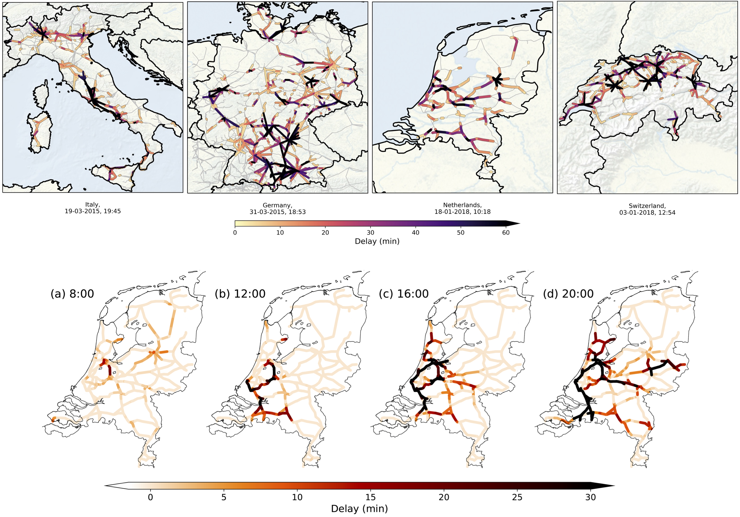
Figure 1: Examples of system-wide disruptions in rail transport: Italian, German, Dutch and Swiss Railways (top panel, from left to right). Italy: near-simultaneous occurrence of several problems in the Italian railways in March 2015 — a major one around Rome, affecting mostly intercity trains, and one between Milan and Venice. Germany: effect of cyclone ‘Niklas’ (31 March 2015) on the German railways. In particular, a specific train near Pegnitz (center-south) was severely damaged by a fallen tree and the rooftop of the Munich station was destroyed, along with multiple smaller incidents across the country. The high risk of more accidents and delays caused the Deutsche Bahn to cancel most of its train activity throughout the day, leaving passengers stranded in major cities like Hannover, Frankfurt, Kassel and Berlin. Netherlands: aftermath of storm ‘Friederike’ in January 2018 in the Netherlands, coinciding with an accident in the north of the country. Fallen trees and damaged overhead lines made the fire department force the Dutch railways to close at multiple stations—resulting in no train activity between the end of the morning and 14:00. Switzerland: in January 2018 (coinciding with storm Burglind/Eleanor in the north-west of Europe) a strong disruption in near Zürich (north) rapidly propagated towards the rest of the country. Albeit caused by external triggers such as weather conditions, power outage etc., system-wide disruptions like these often start localized and small, and systems’ internal operations may even contribute to the growth of disruptions to system-wide scales. System snapshots of the Dutch railways on February 3, 2012 (bottom panel). On that day winter weather conditions from the night before caused scattered service delays early morning [subpanel (a)]. Subsequently, the delays continued to worsen through the day, ultimately resulting in the loss of overview and an eventual shutdown of a significant part of the system [subpanels (b-d)]. Figures and the caption reproduced from Refs. [23] and [5] respectively.

Fragility of socio-technical systems. The overarching concept of fragility has emerged in the last 40 years as a generic property of constrained optimization problems or constraint satisfaction problems [24], like the well-known Traveling Salesman problem [25] or the Max Cut problem [26], also known as the Spin-Glass problem [25] in physics literature. Many problems in STSs are of similar nature: either through the efforts of system operators or by betting on the virtue of an invisible hand, such systems strive to achieve some kind of optimality, with a large amount of constraints. Indeed, optimizing cost and increasing service frequency constrained to reusing the crew from the incoming trains for outgoing trains, as well as input-output production networks – where each firm attempts to maximize profits by appropriately choosing its suppliers and production technologies to match demand from its customers while minimizing inventories – are real-world, and complex, examples of constrained optimization problems.

Such optimization problems typically exhibit fragility in the following sense: the optimal solutions evolve “chaotically” with the precise specification of the parameters of the problem. In other words, the optimal solution for one choice of parameters can become sub-optimal, or even suddenly disappear when these parameters are only slightly changed. Note that this statement can be made precise in the context of spin-glasses, for example, and holds in the limit of a large number of degrees of freedom (for example number of firms, of agents, or of assets, etc., see, e.g. [25]). Such parameter chaoticity is related to the existence of a large number of quasi-optimal solutions, that are nearly equally good in terms of their performance but very different from one another in terms of their realizations (e.g., the actual supplier-client connections in a production network) [27]. Moreover, in a large variety of cases, the optimal solution is found to be sitting, proverbially, “at the edge of a cliff”, in the sense that small perturbations may catastrophically degrade the performance of the system. Such perturbations can either be exogenous [10, 28], namely of origin external to the system, or endogenous [29], meaning they originate within the system. Returning to the train system, a global power failure, or a snowstorm, is clearly an exogenous perturbation, while a mechanical dysfunction of a single train (e.g., due to maintenance issues), or the unavailability of a single crew member, causing a delay, is an endogenous one that may reverberate through the entire system. The boundary between perturbations of exo- vs endogenous origins is, however, not always discernible [6], as seen in Fig. 1.

Operators of STSs therefore have a natural tendency to perceive certain safeguards ensuring stability and resilience as unnecessary hindrances to achieving ever higher efficiency. Further to this, this tendency is particularly strong when the STS has displayed stability for a long time, making such safety measures or regulations seem unjustified. Driven by the desire to optimize, they come to dismantle these safeguards, inadvertently edging the system critically close to collapse. This scenario resembles that of Self-Organized Criticality (SOC) [30, 31] (for the case of STSs, it is organized by the operators themselves that are part of the systems), illustrated by a sand pile that keeps growing until its slope becomes so steep that an avalanche occurs, (partly) collapsing the sand pile. This is also the mechanism proposed by Minsky to explain the recurrence of financial crises [32]: regulations limiting the risk of financial institutions are put in place after crashes, only to be progressively removed as the memory of the last crisis fades.

Further, in systems of systems such as a cluster of interdependent production firms, whose individual operations are intricate systems in themselves, it is foreseeable that competitive pressures force individual firms to aggressively optimize for their own cost and time efficiencies. When such myopic optimization is done simultaneously by many firms — essentially all of them because of competitive pressures — the entire production system will be pushed to the cliff edge (Fig. 2), and will become fragile. Arguably, the more myopic the optimizations, the higher the fragility of the system in its entirety.

Figure 2: A cartoon impression of a STS operator, prompted by incentives (financial or other), attempting to myopically optimizing the system, and in that process, inadvertently pushing the system towards the proverbial cliff edge.

“The trinity” for socio-technical systems: efficiency, fragility and criticality. The location of the constrained optimized solution at the edge of a cliff — that is at criticality — is a property of the whole system, not of its individual parts. Translated to STSs, the Minsky scenario is the following: stable times myopically lower the risk perception of the operators primarily caring about their specific sub-system, and induce them to optimize aggressively. For example, the dispatcher at a given train station might want to reduce the temporal buffer between the incoming and outgoing trains for improving efficiency, but when such local optimizations are implemented system-wide, they will (inadvertently, but structurally) embed fragility, in the sense that even a small delay of an incoming train at one station will cascade and reverberate through the entire system. In the case of production firms that need to buy raw materials from their suppliers in order to produce and sell to their clients, the problem can manifest itself in different ways. Firms may indeed organize their supply chain to reduce the number of redundancies, and may concentrate the sourcing of their inputs on a few key suppliers and goods. When these inputs cannot easily be substituted, either because of physical constraints in the firm’s production (e.g., a chemical plant cannot produce without having energy for its ovens) or because of the difficulty in sourcing them from another supplier (e.g., because of geographic constraints), then the entire economy can become fragile to exogenous shocks as well as prone to amplifying endogenous fluctuations. The first case, when firms cannot easily substitute different types of inputs in their production, is particularly acute when a firm cannot produce at all if a critical input is unavailable.

The degree of substitutability of the production system has been the subject of very animated debates regarding the impact to European economies of receiving less gas from Russia as a consequence of the war in Ukraine, see e.g. Ref. [33].

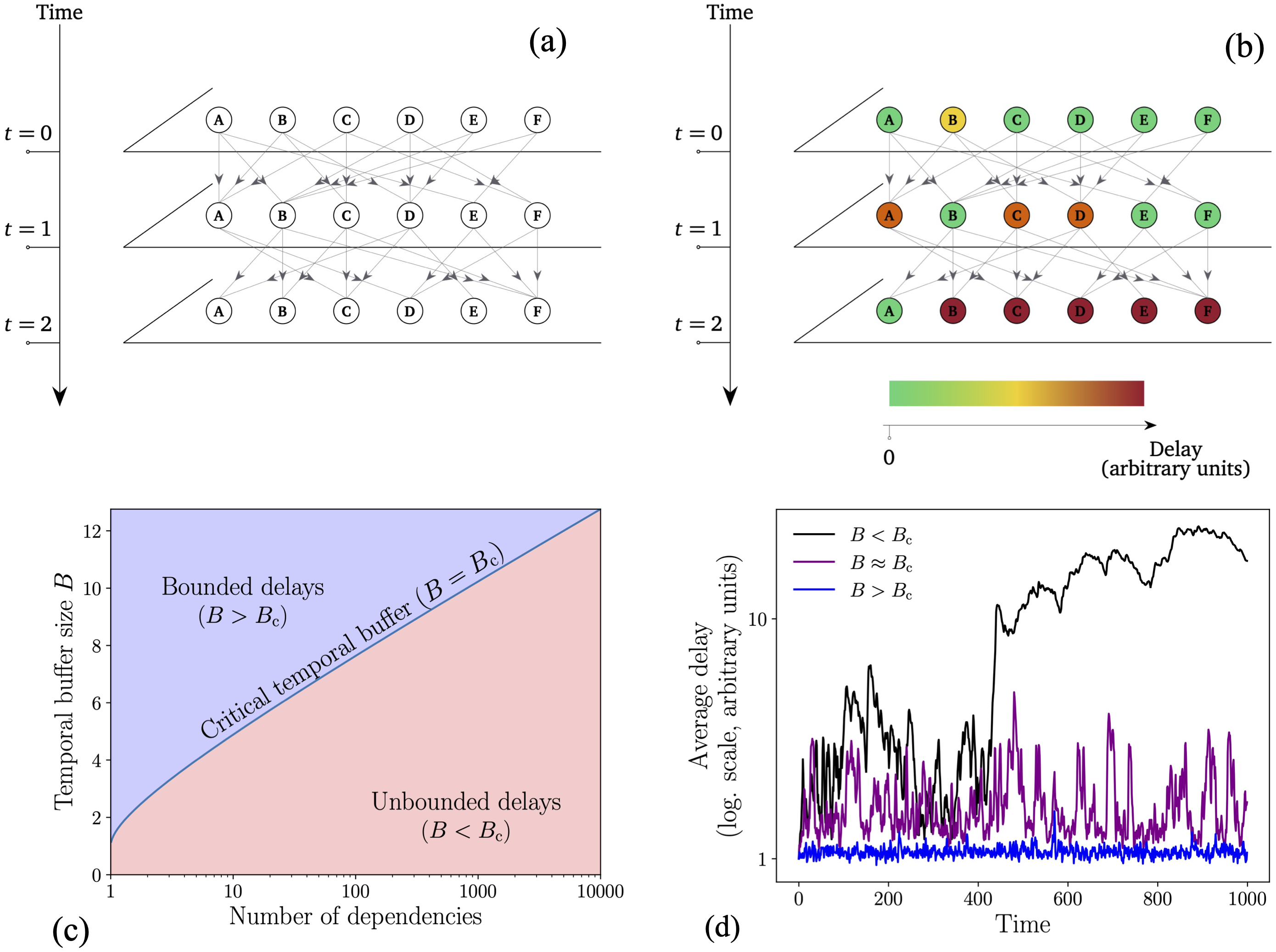
Figure 3: A stylized model for the operations of a firm-to-firm production network. (a) Six firms, A through F, and their operational dependencies across successive temporal layers shown by arrows. (b) An illustration of color-coded production delays propagating downstream in time through this operational dependencies in the network. (c) The temporal criticality curve in the phase diagram of temporal buffer size $B$ and number of dependencies, for the case when each firm has exactly the same total number of operational dependencies. (d) Typical evolution of average delay per firm below, at and above temporal criticality, for the case (c), as a function of time. Note in particular the delay avalanches at $B\approx B_{\text{c}}$.

Temporal criticality. Bringing timeliness, the universally-adopted quality standard for STSs, into the picture, we expect the proximity to criticality of constrained optimized solutions to manifest itself in terms of the system’s propensity to accumulate and propagate of operational delays that may run out-of-control. Indeed, this is an overarching aspect of STSs ranging from financial markets (e.g., liquidity not available when and where needed), to transport (e.g., physical trains/planes or crew members not present at the start of a scheduled service), to production (e.g., raw materials not available at firms when goods need to be produced), to food systems (e.g., grain has not arrived in time at the port for shipping). Specifically, from statistical physics, we expect the systems to be extremely sensitive to delays close to criticality — the closer the system is to the cliff edge, the higher the magnitudes of the delays, and the longer their persistence. We foresee such behavior to be characterized as critical behavior in the temporal dimension, and coin the term temporal criticality to describe it. With increasing proximity to the edge of the cliff, we expect temporal criticality to be associated with diverging correlation times in a power-law fashion.

These ideas can be given a precise form by means of a stylized model (Fig. 3, for a firm-to-firm production network) that describes the propagation of delays across a (spatio-)temporal network of tasks, mimicking the geographical spread and temporal ordering of planned operational interactions among the components of STSs [34]. Note that from the perspective of analyzing STSs as networked complex systems it is natural to employ temporal networks [35, 36] — networks whose topology changes in time — to describe the operations of STSs by encoding the time-varying interactions among the system elements. A temporal network representation of the operations of an STS allows for easy comparison between the planned operation and the transpired operation by comparing their respective topologies. The delay at a certain node of the temporal network is given by a random variable (modeling unexpected events specific to that node) plus the maximum delay of its incoming nodes, from which is subtracted a temporal buffer value $B$. When the second term is negative, the temporal buffer suffices to absorb all accumulated delays at that temporal node, and this contribution is set to zero. This simple model displays precisely the type of behavior described above: there exists a critical temporal buffer value $B_{c}$ below which delays keep accumulating, leading to a system wide crisis. Just above $B_{\text{c}}$, delay avalanches of all sizes appear spontaneously, with no relation to the amplitude of the initial perturbations. Since maintaining buffers entails costs for the operators of STSs, one expects the systems to operate close to $B_{\text{c}}$, and therefore to be generically fragile. This is indeed a crucial aspect of input-output networks, which, in order to avoid uncertainties related to production delays, must rewire when some firms go bankrupt or cease to function, like what happened in the Fukushima region after the 2011 tsunami [37].

Volatility as a possible consequence of temporal criticality. Both financial markets and large economies (such as those of the US or of the Netherlands, see Supplementary Information for the latter) are known to be much more volatile than what would be expected from economic equilibrium models based on rational expectations. These observations are usually referred to as the “excess volatility puzzle”, or the “small shocks, large business cycle puzzle” [38, 13]. Several scenarios have been proposed to explain these effects, see e.g. [39]. One possibility, highlighted by Acemoglu, Carvalho and others (see Ref. [20] for a recent review), is the role played by input-output networks. However, their model does not account for temporally cascading delays that — we posit — are crucial to understand the unfolding of economic crises. Rather, a potent cause of such large scale disruptions may be the “temporal criticality” developing on production networks: operating close to temporal criticality, the network is highly susceptible to delays that lead to a demand-supply imbalance, and price volatility is then simply a response to the demand-supply imbalance. Similar scenarios have been studied through agent-based modelling [40, 41] This echoes, but makes much more precise, the idea of SOC for economic systems first proposed by the late Per Bak and his coauthors in 1993 [30], and revisited by two of us [42].

More work, both theoretical (on realistic models of temporal criticality in supply chains) and empirical (looking for signatures of temporal criticality in production data), is obviously needed to affirm or contradict our posit. We believe that quantifying the role of temporal criticality is a very important research question, both in the economic context and more generally, in the overarching context of STSs.

Concluding remarks. Elucidating the very mechanisms leading to instabilities, failures and system-wide crises in socio-technical systems is crucial to finding remedies, mitigation measures and proposing adequate regulations. Indeed, as we have argued, system optimality and robustness of the solution to small perturbations may be incompatible with each other. One may even go further and state that in many socio-technical systems, myopic optimizations lead to instabilities. Any welfare function that a system operator seeks to optimize should thus contain a measure of resilience, for example, the robustness of the solution to small perturbations, or to the uncertainty about the value of the parameters. Adding such a resilience penalty will for sure increase costs and degrade strict economic performance, but will keep the solution at a safe distance away from the cliff edge. As argued by Taleb [43], and also using a different language in Ref. [44], good policies should ideally lead to “anti-fragile” systems, i.e., systems that spontaneously improve when buffeted by large shocks.

Author contributions. J-PB and DP conceptualized temporal criticality. J-PB, JM and DP analyzed temporal criticality. All authors contributed to the manuscript.

Competing interests. The authors have no competing interests to declare.

References

Supplementary Information

A. empirical evidence for excess volatility in GDP

Despite the fact that GDP volatility is commonly associated with developing economies, this does not mean that it is completely absent in mature economies. As an explicit example of this, consider the Netherlands for which there is good quality open access data on its GDP and also on the value of imported goods, going back a century (with a hiatus in the period 1940-1945). For the GDP there is in addition a time series with quarterly cadence since 1995 [45]. Also, there is a time series for the value of imported goods with a monthly cadence from 2015 [46]. Collectively these time series allow for a determination of volatility on different time scales where the GDP time series provides a more comprehensive picture of the Dutch economy as a whole, whereas the time series for imported goods is already much more closely linked to the issues of buffer sizes for goods, although of course even this is still aggregated over many different types of goods.

In Table 1 some summary statistics are given for the various time series, where the entries ‘Imports’ refer to the total value of imported goods to the Netherlands from all other European countries. While data is available before 1950, it is considered preferable for this analysis to limit the analysis to an epoch without any break. The growth rate is determined from a least squares fit of the logarithm of the variable as a function of time. In addition a high pass filter is applied, which is equivalent to fitting a smooth slow periodic component representing what is akin to economic cycles, and subtracting this. The residual time series, after subtracting the trend and slow cycle components, is therefore most close to what the term volatility intuitively refers to. For that set of measurements of the time series of residuals the Mean Square is calculated (column MSR in table 1) and also the Kurtosis (KR). In the course of this analysis, it is noted that the quarterly cadence GDP residual time series has a rather strong remaining seasonal pattern, which may in part be due to aspects of data collection rather than intrinsic variations. This seasonal modulation is suppressed by half.

Table 1: Volatility in National Accounts data for the Netherlands. Source: CBS open data

series	cadence	epoch	n	growth rate	MSR	KR
				[yr-1]
GDP	annual	1950-2022	72	0.0681	0.0402	0.3293
GDP	quarterly	1995-2022	112	0.0331	0.0184	0.3074
Imports	annual	1950-2022	72	0.0754	0.0744	0.7229
Imports	monthly	2015-2022	96	0.0554	0.0463	0.1990

The MSR for all four series is very similar in value to the growth rates, with less than a factor of 2 between them. In this sense the volatility of each series is substantial. In a formal sense there is also excess volatility in that the kurtosis (column KR in the table) is $>0$ for every time series. This implies that the distribution function of the residuals is heavy tailed and in excess of what normally distributed residuals would show. Comparing the kurtosis for the two different cadence GDP time series shows that these are comparable, so that it would appear that while the (global) economic slowdown is clearly seen, the volatility is present throughout and does not vary. However, in particular the kurtosis for the quarterly cadence GDP time series is very sensitive to that suppression of the seasonal component, so this result should be treated with some caution. The time series for the Imports do not suffer from this issue and there it appears that the monthly cadence time series has a substantially lower kurtosis than the annual cadence one. If the volatility behaves as power-law noise with less power at higher frequency this should be reflected in the time series measured with different cadences. To quantify this, the amplitude, and hence kurtosis might be $K(f)\propto f^{-\alpha}$. Although there are only two cadences of measurement available and therefore no possibility for checking the robustness on these data alone, the results obtained are consistent with such a power-law behavior, with $\alpha=\frac{1}{2}$.

B. Relevant stochastic process models

It is a well-known phenomenon in statistical physics that near a critical point, multiple distinct phases, with the same free energy, are equally acceptable for an overall minimal energy state of the system, which means there is no obstacle for large subdomains to be formed where one or another state dominates. Therefore, small or even microscopic fluctuations in the system can lead to large macroscopic effects, i.e. large fluctuations. The first quantitative treatment of this goes as far back as 1937 [47]. Ising models used for modeling spontaneous magnetization exhibit this behavior, and of course there are physical systems such as spin-glasses and spontaneous electric fields of thin films [48], which do, too. Those same notions of critical behavior leading to large fluctuations have also been applied in STSs to explain behavior such as the stock market crash of 1987, and more generally for financial markets [49]. Also at the level of the entire economy of countries, there is an excess volatility puzzle [50, 51, 52]. It is also known that external shocks cannot be the only factor responsible for this volatility (e.g. Ref. [53]).

Another route to statistically characterizing volatility in STSs is through models with appropriate stochastic behavior and developing the large deviations theory for such models. Hawkes processes are a variant on Poisson processes [54]. In these processes the event rate or likelihood per unit time starts off as finite value, as in a Poisson process, but it is modified whenever an event takes place. If for instance at each event the rate is increased, this leads to cascades of events. If the modification of the event rate is itself drawn from a distribution function, more complex behavior can ensue. The intervals between events are therefore not iid distributed in Hawkes processes. In their linear form, Hawkes process theory has been applied to financial markets [55], but also in a modified quadratic form, which is more realistic [56] since it builds in some of the observed properties of memory effects and hence time-reversal asymmetry in financial market behavior.

The central question is to examine the influence of buffers in large deviations theory and whether such tails become prominent only at zero temporal buffer size, or finite buffer size, and what the role in this is of the network connectivity of the STS on which the process takes place. This is an important avenue for future research.

References

- [1] M. Kaur, L. Craven, Handbook of Engineering Systems Design (Springer, Cham, 2023), chap. Systems Thinking: Practical Insights on Systems-Led Design in Socio-Technical Engineering Systems, pp. 1–29.
- [2] O. L. De Weck, D. Roos, C. L. Magee, Engineering systems: meeting human needs in a complex technological world (MIT Press, 2011).
- [3] W. B. Rouse, Modeling and visualization of complex systems and enterprises: explorations of physical, human, economic, and social phenomena (Wiley, 2015).
- [4] R. Jervis, System Effects: Complexity in Political and Social Life (Princeton University Press, 1997).
- [5] M. M. Dekker, D. Panja, PLOS One 16, e0246077 (2021).
- [6] M. M. Dekker et al., Public Transport 14, 5 (2021).
- [7] S. H. Chung, H. Ma, H. K. Chan, Risk Analysis 37, 1443 (2017).
- [8] J. Sterman, Management Science 35, 321 (1989).
- [9] Newsweek, Southwest airlines nationwide grounding: What we know (2023). Downloaded on May 26, 2023.
- [10] C. Shughrue, B. Werner, K. C. Seto, Nature Sustainability 3, 606 (2020).
- [11] D. J. Lynch, The Washington Post, Suez canal mishap puts battered supply chains under more pressure (2023). Downloaded on May 26, 2023.
- [12] D. Sornette, Why Stock Markets Crash: Critical Events in Complex Financial Systems (Princeton University Press, 2017).
- [13] B. S. Bernanke, T. F. Geithner, H. M. Paulson Jr., Firefighting: the financial crisis and its lessons (Penguin, 2019).
- [14] E. Jaques, The changing culture of a factory (Routledge, 2002).
- [15] F. E. Emery, E. L. Trist, Human Relations 18, 21 (1965).
- [16] G. Baxter, I. Sommerville, Interacting with Computers 23, 4 (1965).
- [17] M. Nesari, M. Naghizadeh, S. Ghazinoori, M. Manoochehr, Technology in Society 68, 101834 (2022).
- [18] S. V. Buldyrev, R. Parshani, G. Paul, H. E. Stanley, S. Havlin, Nature 464, 1025 (2010).
- [19] Y. Sugimori, K. Kusunoki, F. Cho, S. Uchikawa, The international journal of production research 15, 553 (1977).
- [20] V. M. Carvalho, A. Tahbaz-Salehi, Annual Review of Economics 11, 635 (2019).
- [21] R. Lafrogne-Joussier, J. Martin, I. Mejean, IMF Economic Review 71, 170 (2022).
- [22] G. Di Bella, et al., IMF Working Papers 2022 (2022).
- [23] M. M. Dekker, D. Panja, H. A. Dijkstra, S. C. Dekker, PLOS One 14, e0217710 (2019).
- [24] S. Franz, G. Parisi, M. Sevelev, P. Urbani, F. Zamponi, SciPost Physics 2, 019 (2017).
- [25] M. Mézard, G. Parisi, M. A. Virasoro, Spin glass theory and beyond: An Introduction to the Replica Method and Its Applications, vol. 9 (World Scientific Publishing Company, 1987).
- [26] G. Ausiello, et al., Complexity and approximation: Combinatorial optimization problems and their approximability properties (Springer Science & Business Media, 2012).
- [27] C. Colon, J.-P. Bouchaud, Available at SSRN 4300311 (2022).
- [28] H. Inoue, Y. Todo, Nature Sustainability 2, 841 (2019).
- [29] A. Wehrli, D. Sornette, Scientific Reports 12, 18895 (2022).
- [30] P. Bak, K. Chen, J. Scheinkman, M. Woodford, Ricerche economiche 47, 3 (1993).
- [31] P. Bak, C. Tang, K. Wiesenfeld, Phys. Rev. Lett. 59, 381 (1987).
- [32] H. P. Minsky, Can “it” happen again?: essays on instability and finance (Routledge, 2015).
- [33] B. Moll, M. Schularick, G. Zachmann, Not even a recession: The great german gas debate in retrospect, Tech. rep., University of Bonn and University of Cologne, Germany (2023).
- [34] M. M. Dekker, R. D. Schram, J. Ou, D. Panja, Physical Review E 105, 054301 (2022).
- [35] P. Holme, J. Saramäki, Physics Reports 519, 97 (2012).
- [36] P. Holme, J. Saramäki, Temporal networks (SpringerLink, 2013).
- [37] V. M. Carvalho, M. Nirei, Y. U. Saito, A. Tahbaz-Salehi, The Quarterly Journal of Economics 136, 1255 (2021).
- [38] B. S. Bernanke, M. Gertler, S. Gilchrist, The Review of Economics and Statistics 78, 1 (1996).
- [39] X. Gabaix, Econometrica 79, 733 (2011).
- [40] S. Hallegatte, Risk Analysis 34, 152 (2013).
- [41] C. Colon, S. Hallegatte, J. Rozenberg, Nature Sustainability 4, 209 (2020).
- [42] J. Moran, J.-P. Bouchaud, Physical Review E 100, 032307 (2019).
- [43] N. N. Taleb, Antifragile: Things that gain from disorder, vol. 3 (Random House Trade Paperbacks, 2014).
- [44] W. Hynes, D. Trump, B. D. Kirman, A. Haldane, I. Linkov, Nature Physics 18, 381 (2022).
- [45] Statline open data: Bbp, productie en bestedingen; kwartalen, waarden, nationale rekeningen, Tech. rep., Statistics Netherlands (2023).
- [46] Statline open data: Internationale goederenhandel; eigendomsoverdracht, kerncijfers, Tech. rep., Statistics Netherlands (2023).
- [47] L. D. Landau, Zh. Eksp. Teor. Fiz. 7, 19 (1937).
- [48] A. Cassidy, F. P. Pijpers, D. Field, J. Chem. Phys. 158, 144501 (2023).
- [49] T. Bury, Journal of Statistical Mechanics: Theory and Experiment p. P11004 (2013).
- [50] G. W. Schwert, The Journal of Finance 44, 1115 (1989).
- [51] P. Bak, K. Chen, J. Scheinkman, M. Woodford, Ricerche Economiche 47, 3 (1993).
- [52] N. V. Loayza, R. Rancière, L. Servén, J. Ventura, World Bank Economic Review 21, 343–357 (2007).
- [53] C. Raddatz, Journal of Development Economics 84, 155–187 (2007).
- [54] A. G. Hawkes, Biometrika 58, 83–90 (1971).
- [55] A. G. Hawkes, Quantitative Finance 18, 193–198 (2018).
- [56] P. Blanc, J. Donier, J.-P. Bouchaud, Quantitative Finance 17, 171 (2017).